DFG-Schwerpunktprogramm 1114 Mathematical methods for time series analysis and digital image processing

Mathematical methods for forecasting

bank transaction data

P. Maaß T. Köhler J. Kalden R. Costa

U. Parlitz C. Merkwirth U. Wichard

Preprint 24

Preprint Series DFG-SPP 1114

Preprint 24 January 2003

2

Mathematical methods for forecasting bank transaction data

Peter Maass1, Torsten Koehler1, Jan Kalden2, Rosa Costa3, Ulrich Parlitz4, Christian Merkwirth4, Jörg Wichard4

Abstract

We aim at comparing different methods for forecasting several types of credit card transaction data. These data can be devided into two groups – one of them is characterised by a distinctive structure (trend, seasonality) but with very short data bases, the other one is larger but high volatile. Evaluated methods include those from statistics and nonlinear dynamics as well as wavelet techniques. Beside the software developed for this purpose standard toolboxes for time series analysis have been applied.

1. Introduction

1.1 Starting point

Forecasting market trends (prices, volumes, and numbers) is of great importance for many direct and indirect economical processes within companies. Examples of these processes are the prediction of the number of calls that need to be processed according to the defined service level agreements and the CPU-times needed to facilitate debit and credit card transactions.

In practice decisions are made mainly on an intuitive basis and on assumptions, without having precise quantitative analyses available. This leads to an incorrect decision-making process. The costs of these decisions are intense.

However, accuracy, timeliness and reliability deriving from the present in-place forecasting methods can be improved. Further investigations show us that the interpretation and the forecasting of trends are depending on the level of knowledge and the abstraction level that analysts and managers have.

At present, the existing data base of Interpay is primarily used to extract statistical information on different kinds of data as total volume of transactions, number of bank accounts, number of incoming calls to call centres, number of transactions in different categories, etc. However, a more in-depth analysis of the available data is currently under development.

The final objective of this collaboration is to provide additional services to banks based on a combination of time-series analysis and mathematical modelling of the available data. Such services could include an early detection of trends or a reliable forecast of, e.g., numbers of incoming calls in call centre, which would allow an improved operation of the business units involved. This could be achieved by combining different forecasting methods for obtaining a reliable, adaptive and efficient solution.

1 Universität Bremen, Zentrum fuer Technomathematik (ZeTeM) 2 Interpay Nederland B.V. 3 University of Porto 4 Universität Göttingen, Drittes Physikalisches Institut

3

Here, different scientific methods were compared to show the applicability of these methods with respect to different scenarios and data. Because of this interdisciplinary approach, the different methods are described very explicitly to enhance understanding.

For all that purposes we have evaluated

• different versions of ARMA-models

• wavelet methods

• an ensemble methods based on a competition between different types of basic models including neural networks, RBF-networks, perceptrons, linear regression, local models (exploiting nearest neighbour relations) etc.

• standard tools for time series analysis from statistics and non-linear dynamics as ITSM2000 and TISEAN 2.1 .

2. Time-series forecasting for total volume of transaction data

2.1 Scope

A first study has been done in order to test basic methods on this most reliable but characteristic data set. Doing this, the basis for an ongoing cooperation between Interpay Nederland B.V. and a working group within the DFG-Schwerpunktprogramm “Mathematical methods of time series analysis and image processing” could be developed.

2.2 Methods

This set of data has very nice and strong structures:

• an almost linear trend, which only shifts its inclination over the last year of data

• a highly reliable 12-month periodical structure

This data can be forecasted with high reliability by classical autoregressive AR(L) models.

The downside of this nice structure is, that more sophisticated models do not further enhance the forecast considerably. Furthermore, the data set only contains 51 data points, of which the last 11 were hold back for checking the computed forecast. I.e. only 40 data points can be used to develop the forecasting models.

Because of that reason and in order to not to duplicate work of [7], we have restricted modelling and analysis of the data to of the most standard forecasting models:

• AR(L) model with K autoregression coefficients, the coefficients are chosen such that the resulting time series matches best the first M autocorrelation coefficients of the real data (Yule Walker equations). The choice of the model dimensions were done by information criteria and MAPE estimations.

• AR(L) model with K autoregression coefficients, the coefficients are chosen in order to reproduce the first 40 data points in the time domain optimally (least square estimates)

In addition to these basic methods, we have

4

• applied a wavelet decomposition to the data, to examine the change of trends in the data and to develop a hybrid autocorrelation-wavelet model

• tested ARMA implementations and further options of standard software ITSM2000 for comparison

2.3 Applying an AR(L) model via Yule-Walker equations

2.3.1 Fitting the model

The definition of an autoregression model

xn = a1 x(n-1) + .... + aL x(n-L)

as well as an introduction to the Yule-Walker theory is already contained in [7]. For short time series, e.g. the first 40 data points of the time series, special care has to be taken for adjusting boundary effects. Let Ntest denote the length of the data set available for fitting the AR-model, L denote the dimension of the AR(L) model, K denote the number of autocorrelation coefficients used to determine a1 , .... , aL.

The linear system, which is set up by the Yule-Walker equations, is defined by the autocorrelation coefficient ρ(m) of the time series x1 , .... , xNtest . A careful analysis of the defining equations leads to a small modification. For short time series we want to take the maximal advantage of the available data, hence we adjust the length of the subseries used for computing the autocorrelation coefficients:

rhomat=zeros(ntest-1,ll); rhom0 =zeros(ntest-1,1); sum=0.0; for i=(ll+1):ntest sum=sum+x(i)*x(i); end; rho00=sum; for k=1:(ntest-ll-1) sum=0.0; for i=ll+1:(ntest-k) sum=sum+x(i)*x(i+k); end; rhom0(k)=sum; end; for m1=1:(ntest-ll) rhomat(m1,1)=rhom0(m1)+x(ll)*x(ll+m1); end; for m2=2:ll for m1=m2:ntest+m2-ll-1 rhomat(m1,m2)=rhomat(m1,m2-1)+x(ll+1-m2)*x(ll+1-m2+m1); end; end;

The vector rhom0 contains the classical autocorrelation coefficients. The Yule-Walker matrix is then set up by

aa=zeros(kmax+1,ll); for i=1:kmax for j=1:ll aa(i,j)=rhomat(i+j,j); end; end; for j=1:ll aa(kmax+1,j)=rhomat(j,j); end;

In order to select the dimensions L and K of an autoregression model defined via Yule-Walker equations, we have implemented two basic decision criterion.

5

The Akaike information criterion was computed for each admissible pair (L,K). A small number of the information criterion indicates a good model, for visualisation purposes it is better to plot the inverse numbers, i.e. the maximal value in the plot below indicates the optimal model. Local maxima of the inverse Akaike information indicate good models for the underlying time series.

Secondly we computed the differend MAPE values of all admissible (L,K) pairs, but only using the first 40 data values. Again a small number indicates a good model, hence we have plotted the inverse numbers for a better visualization. Based on these criteria, we have selected four (L,K)-models: (L=12, K=5), (L=15, K=20), (L=16, K=12), (L=18, K=19). The resulting autoregression coefficients a1 , … , aL are given in Table 1.

L=12, K=5 L=15, K=20 L=16, K=12 L=18, K=19

YW TD YW TD YW TD YW TD 1 0.0938 0.0334 0.7074 0.1513 -0.0899 0.3146 2 0.4248 -0.0558 -0.1448 0.2541 0.0541 -0.1461 3 -0.0320 0.0787 0.3815 0.2000 0.5300 0.2982 4 -0.2589 -0.1726 -0.0794 -0.0245 0.1723 0.2364

5 0.3046 0.1347 0.3337 0.3489 0.1821 -0.1346 6 -0.2759 -0.0358 -0.1952 -0.1902 0.0089 0.1734 7 -0.0136 -0.0020 0.0064 -0.0171 0.0189 0.1261 8 0.0439 -0.0619 -0.0520 -0.1022 -0.0657 -0.0183 9 0.0033 0.0423 0.1131 0.1811 -0.0318 0.0293

10 0.0383 0.0106 -0.2617 -0.0921 0.0282 -0.2224

Figure 2: Inverse MAPE, computed over the first 40 value, the axis to the right denotes K=number of correlation coefficientes, the axis to the left L=number of autoregression coefficients

Figure 1: Inverse Akaike information criterion, the axis to the right denotes K=number of correlation coefficientes, the axis to the left L=number of autoregression coefficients

6

11 0.1710 0.0230 0.3077 0.0126 0.0437 0.2764 12 0.5517 1.0722 0.8896 1.0184 1.0749 0.8990

13 -0.6717 -0.0102 0.1248 -0.3125 14 0.2638 -0.1475 -0.0855 0.3334

15 -0.6037 -0.3956 -0.5532 -0.5063 16 -0.1780 -0.4105 -0.4121 17 0.5083 18 -0.4433

Table 1: Autoregression coefficients, Yule-Walker (YW), timedomain estimation (TD)

MAPE MAPE MAPE MAPE MAPE

n=first 3 n=first 4 n=first 6 n=last 6

L=12, K=5 0.1092 0.0536 0.0562 0.1033 0.1311

L=15, K=20 0.0579 0.0688 0.0774 0.0621 0.0459

L=16, K=12 0.0875 0.0339 0.0638 0.0932 0.0829

L=18, K=19 0.0440 0.0611 0.0689 0.0507 0.0347

TD L=12 0.0728 0.0594 0.0882 0.0798 0.0558

TD L=16 0.0545 0.0492 0.0707 0.0653 0.0414

Table 2: Different MAPE values for all tested models

2.3.2 Forecasting using the Yule-Walker AR(L) model

We have used all four models, for forecasting the data for n = 41 , ... , 51 . Comparing these results with the true values gives a MAPE as stated in Table 2. The plots of these forecasts are displayed in Figures 3, 4, 5 and 6.

95% error bounds are computed via a Monte Carlo simulation: An autoregression model of dimension L requires starting values xn for n = Ntest–L+1 , ... , Ntest in order to forecast value xn with n > Ntest .

Hence we have added noise (random numbers, N(0,1) distributed, error level estimated from the previous data points) to the required starting values and repeated the forecasting with these values. This procedure was repeated 1000 times with different random errors, the resulting 95% error bounds of the forecast are plotted below in Figures 7, 8, 9 and 10.

The error level was computed by the prediction error of the first 40 data points, i.e. the models were tested with an error level of 10%.

Figure 3: Forecast (left) and error bounds (right) of transaction data using an AR(L) model determined via the Yule-Walker equations with L=12, K=5

7

Figure 4: Forecast (left) and error bounds (right) of transaction data using an AR(L) model determined via

the Yule-Walker equations with L=15, K=20

Figure 5: Forecast (left) and error bounds (right) of transaction data using an AR(L) model determined via

the Yule Walker equations with L=16, K=12

Figure 6: Forecast (left) and error bounds (right) of transaction data using an AR(L) model determined via

the Yule Walker equations with L=18, K=19 2.4 Applying an AR(L) model via a least square fit in the time domain

2.4.1 Choosing the model

As in the previous section we consider an autoregression model

xn = a1 x(n-1) + .... + aL x(n-L)

8

The coefficients a1 , ... , aL are now chosen s.t. the prediction over the range of the test data is best, when measured by mean squared errors. This leads to a symmetric linear system of equations with matrix aa and right hand side b as described below.

aa=zeros(ll,ll); b=zeros(ll,1); for j=1:ll for l=1:ll sum=0.0; for n=ll+1:ntest sum=sum + x(n-l)*x(n-j); end; aa(l,j)=sum; end; end; for j=1:ll sum=0.0; for n=ll+1:ntest sum=sum+x(n)*x(n-j); end; b(j)=sum; end;

Such a model is determined by one parameter, namely the number L of autoregression coefficients, alone. In order to select the parameter L we have again considered the same two basic decision criterion.

This leads in both cases to dimensions L = 12 or L = 16 , which are good choises for the model parameter. The resulting autoregression coefficients a1 , ... , aL are given in Table 1. It is remarkable that the chosen autoregression coefficients differ considerably between YW and TD models. 2.4.2 Forecasting using the time-domain AR(L) model

We have used both models, L = 16 and L = 12 for forecasting the data for n = 41 , ... , 51. Comparing these results with the true values gives a MAPE stated in Table 2. The requested 95% bounds are computed via a Monte Carlo simulation as described in the previous section.

The model was tested with the same error level as above.

Figure 7: Forecast (left) and error bounds (right) of transaction data using an AR(L) model determined via a

time domain least square fit with L = 12

9

Figure 8. Forecast of the data using an AR(L) model determined via time domain least square fit with L = 16 The average error is below 10 %, which is of the order of the data error. This result can be achieved even for forecasting the data of the last year, when the peak is not as pronounced as in the previous year and the linear trend has changed, too.

2.5 Analysing transaction data by wavelet methods

Wavelet methods are particularly suited to detect local features in a time series. E.g. a change of a linear or exponential trend is regarded as a local structure at the time instant were it occurs first. However, wavelet methods require finely sampled, long data sets. They rely on a decomposition of the time series in a series of detail subsignals on varying scales of size. The usual scaling uses a subsampling by a factor of 2, i.e. a time series of length 512 is reduced to a series of length 8 after only six iterative decomposition steps.

In addition, wavelet methods should be used as an additional tool to model time series only if classical methods fail. A good descritption of such wavelet models for times series analysis is contained e.g. in [2].

The data can already be predicted with high reliability with basic AR-models, even ARIMA, ARMAX, Prony, etc. models do not add significantly new information. Therefore we have restricted the wavelet analysis to one question, namely to predict the linear trend underlying this data set. Applying a wavelet analysis, however, gives a local estimate of the trend at each time instant, it can therefore detect changes of trend at it’s first occurence.

10

Figure 9: Wavelet decomposition of the given transaction data of 51 data points. The computed data a4 displays the linear trend, which changed around data point 38, d3 shows the non-stationary seasonal component.

Figure 10: Subtracting the non-stationary wavelet trend leads to detrended data (left), which is forecasted

using a time domain model with L=16 (right).

2.6 Applying ITSM 2000

Furthermore, we have tested the commercial software package ITSM 2000 (version 7.0) by P.J. Brockwell and R.A. Davis. For a broad comparison several forecasts strategies have been tested. Those are described here just in a very short manner, for further explanation see [1].

I. An extention of the Holt-Winters Forecast Algorithm in order to consider a seasonality with known period (SHW):

11

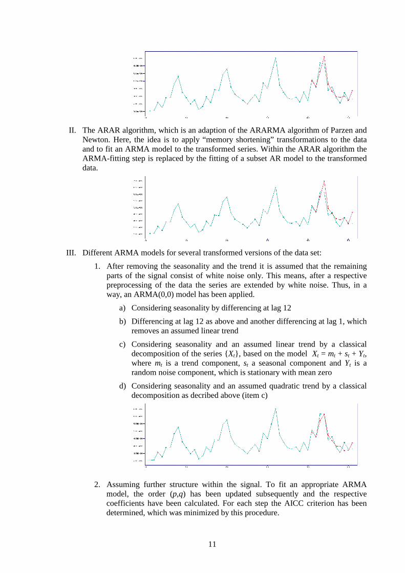
II. The ARAR algorithm, which is an adaption of the ARARMA algorithm of Parzen and Newton. Here, the idea is to apply “memory shortening” transformations to the data and to fit an ARMA model to the transformed series. Within the ARAR algorithm the ARMA-fitting step is replaced by the fitting of a subset AR model to the transformed data.

III. Different ARMA models for several transformed versions of the data set:

1. After removing the seasonality and the trend it is assumed that the remaining parts of the signal consist of white noise only. This means, after a respective preprocessing of the data the series are extended by white noise. Thus, in a way, an ARMA(0,0) model has been applied.

a) Considering seasonality by differencing at lag 12

b) Differencing at lag 12 as above and another differencing at lag 1, which removes an assumed linear trend

c) Considering seasonality and an assumed linear trend by a classical decomposition of the series { Xt} , based on the model Xt = mt + st + Yt, where mt is a trend component, st a seasonal component and Yt is a random noise component, which is stationary with mean zero

d) Considering seasonality and an assumed quadratic trend by a classical decomposition as decribed above (item c)

2. Assuming further structure within the signal. To fit an appropriate ARMA model, the order (p,q) has been updated subsequently and the respective coefficients have been calculated. For each step the AICC criterion has been determined, which was minimized by this procedure.

12

a) Data preprocessing as described at item 1.d leads to a fit of an ARMA(3,3) model with the following coefficients:

3.00E+06 3.50E+06 4.00E+06 4.50E+06 5.00E+06 5.50E+06 6.00E+06 6.50E+06

0 10 20 30 40 50

b) Direct fitting of an ARMA model as described above leads to a similar result using a model of order (13,1):

c) Fitting the best pure AR model (i.e. restricting q being 0) leads to a model of order 16, which was the best result of all fitted models.

i AR coefficients

1 -0.0530 2 0.0763 3 0.3751 4 0.3340 5 0.1330 6 -0.0457 7 -0.0458 8 -0.0487 9 -0.0314 10 -0.0091 11 0.1600 12 0.8130 13 -0.0009 14 -0.0805 15 -0.4100 16 -0.4390

i pi qi 1 -0.4278 0.2624 2 -0.1527 -0.2597 3 0.7184 -0.9988

i pi qi 1 0.9351 -0.9400 2 0.0785 3 0.0262 4 -0.1643 5 0.1813 6 -0.1164 7 -0.0019 8 0.0170 9 -0.0039 10 -0.0455 11 0.2143 12 0.6757 13 -0.8638

13

3.00E+06

3.50E+06

4.00E+06

4.50E+06

5.00E+06

5.50E+06

6.00E+06

6.50E+06

0 10 20 30 40 50

The following table summarises the results of the different forecasting strategies.

ITSM Modell

I. II III.1.a III.1.b III.1.c III.1.d III.2.a III.2.b III.2.c best result from 2.25

MAPE value %

6.19 7.33 6.36 6.26 6.82 5.84 4.64 4.67 4.30 4.40

3. More specialized data sets describing credit card transactions

We have processed six further data sets describing several aspects of transactions.

We have tested and compared Wavelet Methods as described in paragraph 2.5, an ensemble methods based on a competition between different types of basic models and ITSM 2000. 3.1 Wavelet methods The analysis of these data is based on the methods described in paragraph 2.3 – 2.5, where different versions of AR(L)-models were used to forecast the data and basic wavelet methods were used to analyse the underlying trend of the time series.

The special structure of the data to be analysed now force to extend the wavelet analysis and to apply non-stationary wavelet models in a slightly more sophisticated way. Wavelet decompositions are used, first of all, to detect non-linear, non-stationary trends and non-stationary, quasi-periodic seasonal structures.

Based on these insights we divide the time-series into quasi-stationary pieces, which are subjected to separate further investigations. The data set containing the latest available data points are then used to fit a model and to compute forecasts exceeding the previously available data.

In the following we will explain this by means of one example (Total (monthly) revenue of Mastercard transactions made inside Netherlands by foreign cardholders). The following steps have been accomplished:

• The linear trend was determined using a Haar-wavelet decomposition on five levels. • The periodic structures were obtained by a trigonometric fit to a decomposition with

Coiflet4 on four levels.

5 obtained for L=18, K=19 (see table 2, 4th row, 1st column)

14

The components observed and processed are (adjustment between real data (blue lines) and the structures analysed (green lines) ): �

Linearly increasing trend built with data from January 1998 until the last data point – October 2002:

�12 months and 6 months periodicity:

Beside the 12-month-backward forecast of the comparison given in paragraph 3.4 a forecast for the next 14 month has been done for the user. The result is given in figure 11.

Figure 11. Final forecast of the period between November 2002 and December 2003, with 95% confidence lower and upper bounds.

3.2 Ensemble method

Furthermore, for predicting the temporal evolution of the given financial time series an ensemble approach was used.

Ensemble models [5,8] consist of a variety of individual models that may (and actually should!) differ very much. A (weighted) average of the outputs of all regression models involved provides the desired ensemble prediction. If the errors of the individual models are

��������� � �� ���������� ����������� ����� "!$# %$&('") *,+$-$./&!$0$1 2 3$%$04&(% 54!$640434)

7 8"9 :::"9 :::;(8"9 :::"9 :::<(8"9 :::"9 :::= 8"9 :::"9 :::> 8"9 :::"9 :::

? @ABCED FGBC D @HBC ? IJ BCLK MNBCPO QRBC

? @ABB D FGBB D @HB

B? IJ BB K MNBB O Q RBB

? @ASS D FGSS D @HS

S? IJ SS K MNSS O Q RSS

? @ASTUD FGST D @HST ? IJ STEK MNSTPO QRST

? @ASVUD FGSV D @HSV ? IJ SVEK MNSVPO QRSV

? @ASWUD FGSW D @HSW ? IJ SWEK MNSWPO QRSW

XY&* 64'"Z ) [!4# %$&('")(* \[!$]�%"#�54!$64043 ^,_4_4%"#�54!$64043

15

uncorrelated, the generalization error of the ensemble (on new data from the same source) turns out to be smaller than the mean generalization error of the individual models constituting the ensemble. In this way robust models may be generated that avoid or overcome typical regression problems like overfitting and the bias-variance-dilemma.

The ensemble used for the current study consisted of local nearest neighbor models, radial basis networks, single- and multilayer perceptrons and linear regression. Input to all these models are delay vectors with embedding dimension 12 and lag 1 (i.e., each input vector corresponds to a period of time of one year). The prediction horizon was one month and long term predictions were generated recursively based on previous one-month-predictions.

The generation of the ensemble consists of two parts. The first part is an iterative procedure where in each step the data are divided randomly into a training set (80%) and a test set (20%). Each individual model in the ensemble is trained using crossvalidation providing test errors. Models from this pool whose superposition of output minimizes the error on test data constitute model clusters that are stored as preliminary results of the modelling procedure. Those individual models which turn out to be noncompetitive and thus are not used in a model cluster are neglected. This step of model cluster generation is repeated about 10 times with different random divisions of training and test data resulting in different model clusters.

In the second part the model clusters are evaluated again using their prediction error on the full data set. According to this ranking the (80%) best clusters are selected (with some probability proportional to their ability to model the data) and the individual models contained in these clusters constitute the final model ensemble.

The goal of this two step procedure is to avoid overfitting on the level of model selection. Numerical simulations for the given data were performed with the matlab software package ENTOOL ( http://chopin.zet.agh.edu.pl/~wichtel/ ).

A summary of the results obtained with all the methods applied is given in the following paragraph 3.3. 3.3 Results

Table 3 gives results obtained with the methods described in paragraphs 3.2 and 3.3 together with ARMA forecasts computed with ITSM2000. For these calculations we detained the last 12 points of the overall 59 entries for the subsequent comparison.

Data set Wavelet Ensemble ITSM

MasterCard Retail (foreigners) 9.83% 8.64% 10.21% MasterCard Retail (inhabitants) 5.35% 6.64% 6.96% MasterCard Cash (foreigners) 25.68% 14.38% 22.66% MasterCard Cash (inhabitants) 6.40% 6.46% 7.67% Maestro Retail 11.99% 31.29% 13.90% Maestro Cash 9.32% - 36.28%

Table 3. MAPE values for all the six data sets and the tested methods Figure 12 displays two results for the first data set (MasterCard Retail – foreigners).

16

Figure 12. Forecasting results with wavelet methods (green line) and ensemble method (red line) for data set “MasterCard Retail - foreigners”

4. Forecasting Charge Back Data

4.1 Scope

A Charge Back is a disputed transaction resulting from a previous credit card transaction. The owner of the credit card, after having received his account overview, can file a complaint in which he explains to the charge back department that he did not create the transaction he now disputes. The reasons can vary (“ I was not in Italy” , “My card was just stolen” , “The amount of money is incorrect” , “This is not my autograph”, etc.). The shop owner can also dispute a transaction (the card used in the transaction was not legal, viable, the right amount of money was not received, the card was from somebody else). There are many dozens of reasons why a cardholder or a shop owner may disagree with the transaction overview. This process can stay alive for a considerable time: question, answer, question 2, answer 2 etc. Other parties get involved. Finally legal action can be taken to retrieve the disputed money.

These complicated and long running procedures lead to remarkable financial risk. Thus, their correct prediction is of great importance as well for Interpay as for the banks involved. The data itself is characterized by a high volatility, resulting from the charge back process with all its parameters and delays as described above. Therefore, for the evaluation here we use the mean percentage error (MPE) instead of mean absolute percentage error (MAPE), because the user is interested in weekly or monthly expectations, not in exact daily values.

Again a combination of a wavelet model for fitting the non-stationary trend with an AR(L)-model was used to forecast the data. Furthermore, ITSM2000 has been applied for comparison. Because of the higher number of available data points the application of methods from nonlinear dynamics was also reasonable. Thus test calculations with TISEAN 2.1 have been done.

4.2 Data analysis

4.2.1 General preprocessing

The data do not exhibit significant structures at a first look. Tests for randomness (white noise) based e.g. on evaluating the autocorrelation function or the Fourier power spectrum

17

show values very close to randomness, see Figure 13 and 14. Hence, only a rough forecasting can be expected.

Figure 13 Figure 14 Figure 13 and Figure 14: The plot of the Fourier transform of the original data shows no structure, the absolute Fourier spectrum is almost flat with a comparatively low variance. The plot of the Fourier power spectrum also exhibits no meaningful structure. The data needs substantial preprocessing, before an attempt to forecast this time-series has any chance of success.

During the first few months the data points are rather irregularly sampled, this becomes more consistent towards the end of the considered period. Most of the data points are for weekdays, some refer to Saturdays.

• Preprocessing Step 1: Interpolated data are filled in for the missing weekdays, data for Saturdays are eliminated.

The data exhibits several unreasonable outliers. We use the log-log-criterion to determine a reasonable value for thresholding and eliminating outliers.

Figure 15 clearly indicates a threshold of approx. 2200, i.e. the three largest value of the volume data are eliminated.

Analysing the volume/transaction quotient also shows outliers, they are removed by the same method.

• Preprocessing Step 2: Removing outliers in the volume time-series directly and via the volume/amount-quotient.

Figures 17 and 18 plot the original and the preprocessed data. The preprocessed data set is longer than the original data, since some missing data points had to be filled in at the beginning of the time series. The preprocessed volume data consists of 1212 data points.

The outliers of the original series have been removed.

18

Figure 15 Figure 16

Figure 15: The histogram of the daily volume allows to determine a threshold for the elimination of outliers. The log-plot of the histogram enters a flat region at a daily volume of approx. 2200. This is taken as the threshold for eliminating outliers.

Figure 16: The plot of the quotient of number of charge backs and volume of charge backs also shows outliers, they are eliminated by the same method as eliminating outliers in the original daily volume data set, Figure 16 shows the questions after removing the outliers.

Figure 17 Figure 18 Figure 17: The original data shows strong outliers, it captures a time period from May 1997 to January 2002, the sampling is irregular. Figure 18: The preprocesed data consists of 1212 data points, the last data point refers to January 21 2002. The data set contains five values for each week between May 1997 – January 2002.

4.2.2 Wavelet preprocessing

The output of the three preprocessing steps, as described in the previous section, is still hard to forecast directly. We use a wavelet decomposition with a coiflet of order 4 on 7 scales of decomposition. This wavelet lead to the best results amongst all wavelets, which were tested.

19

200 400 600 800 1000 1200

−400−200

0200400

d1

−400−200

0200400600

d2

−2000

200d

3

−1000

100d

4

−100

0

100

d5

−60−40−20

02040

d6

−200

20d

7

180200220240260280

a7

50010001500

s

Decomposition at level 7 : s = a7 + d7 + d6 + d5 + d4 + d3 + d2 + d1 .

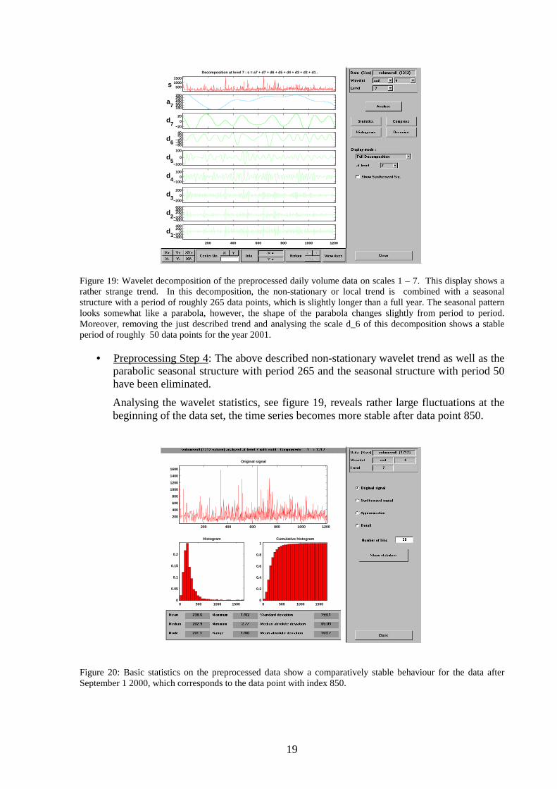
Figure 19: Wavelet decomposition of the preprocessed daily volume data on scales 1 – 7. This display shows a rather strange trend. In this decomposition, the non-stationary or local trend is combined with a seasonal structure with a period of roughly 265 data points, which is slightly longer than a full year. The seasonal pattern looks somewhat like a parabola, however, the shape of the parabola changes slightly from period to period. Moreover, removing the just described trend and analysing the scale d_6 of this decomposition shows a stable period of roughly 50 data points for the year 2001.

• Preprocessing Step 4: The above described non-stationary wavelet trend as well as the parabolic seasonal structure with period 265 and the seasonal structure with period 50 have been eliminated.

Analysing the wavelet statistics, see figure 19, reveals rather large fluctuations at the beginning of the data set, the time series becomes more stable after data point 850.

200 400 600 800 1000 1200

200

400

600

800

1000

1200

1400

1600

Original signal

0 500 1000 15000

0.05

0.1

0.15

0.2

Histogram

0 500 1000 15000

0.2

0.4

0.6

0.8

1Cumulative histogram

Figure 20: Basic statistics on the preprocessed data show a comparatively stable behaviour for the data after September 1 2000, which corresponds to the data point with index 850.

20

2.2.3 Wavelet processing and forecasting

We only consider the cleaned data, in the following analysis. As described above, we delete the final n month ( n = 5 , … , 1 ) before building our model for forecasting data in order to forecast month 8-(n-1).

The previous analysis suggests an additive model, consisting of three components

• Non-stationary, locally parabolic trend • Seasonal mid-scale model, periods approximately 50 data points. • A quasi-noisy times series, with no apparent structure.

These last, quasi-noisy component is displayed in Figure 21.

Figure 21: The quasi- noisy component is the difference between the daily volume data and the smooth wavelet trend. This decomposition is done for the data before November 1 2001 only. According to the previous considerations we now forecast each component separately. The first two components are forecasted in the wavelet domain. The third component is forecasted using an AR(L)-model, which is fitted by a time domain least square method.

• Wavelet models for fitting the non-stationary trend and the seasonal mid-scale component

The following figure displays some significance levels for the wavelet decomposition. We used the following simple and stable forecasting method for he wavelet decomposition on levels d1-d7: Only scale d6 contains significant and stable structures for the last twelve month of data. Hence all scales are forecasted by constant zero values. The scale d6 is forecasted by the average value of the last five significant values, i.e. scale d6 is forecasted by a constant value of 144,3 .

The forecasting of scale a7 is done by a simple periodic continuation.

21

200 400 600 800 1000 1200

500

1000

1500

Original signal

Original coefficients

Leve

l num

ber

200 400 600 800 1000 1200

7

6

5

4

3

2

1

−2000

200

d7

Original details coefficients

−400−200

0200400

d6

−400−200

0200400

d5

−500

0

500

d4

−500

0

500

d3

−1000

0

1000

d2

200 400 600 800 1000 1200

−500

0

500

d1

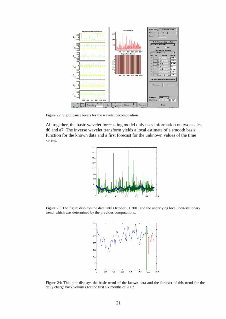
Figure 22: Significance levels for the wavelet decomposition.

All together, the basic wavelet forecasting model only uses information on two scales, d6 and a7. The inverse wavelet transform yields a local estimate of a smooth basis function for the known data and a first forecast for the unknown values of the time series.

Figure 23: The figure displays the data until October 31 2001 and the underlying local, non-stationary trend, which was determined by the previous computations.

Figure 24: This plot displays the basic trend of the known data and the forecast of this trend for the daily charge back volumes for the first six months of 2002.

22

The basic wavelet trend for the data until October 31 2001 is plotted in blue, the 50 data points until January 21 2002 are plotted in green and the six month forecast until June 30 2002 is plotted in red. The last data point corresponds to June 30 2002. It is apparent that the time series is rather unpredictable at the beginning and becomes more stable at the end. At general downward trend is visible in the forecast.

• Intermediate calibration step

The remaining times series, after extracting the wavelet trend has a global mean value zero. In order to adjust the time series to a local mean value zero, we have averaged the remaining quasi-noise component: each data value is adjusted by computing the mean value over ten preceding values. This e.g. gives a correction term of 74,9 for the last available data points before November 1 2001.

• AR(L)-models for fitting the noise component

As usual we perform the following three steps:

- Determination of the model dimension by an information criterion - Fitting the optimal model - Forecasting via the optimal model

The information criterion indicates to use a model of dimension L=5,12 or 27 for fitting the trend, see figure 25. The resulting MPE values for forecasting the noise component over the last 10 weeks (50 data points) is summarised in table 4. As expected, an almost constant forecast indicates, that no significant structure is left in the remaining quasi-noisy component.

Figure 25: The Akaike information criterion indicates a model of dimension 27, other information citeria also suggest at use models of dimension 5 or 12.

Finally we combine the previous three parts (wavelet trend, intermediate calibration, AR(L)-model) to generate a complete model. The resulting MPE values are listed in Table 4.

5 Days 10 Days 20 Days 50 Days L=5, TD 0.3288 0.5175 0.3727 0.3667 L=12, TD 0.4257 0.5394 0.3835 0.3712 L=27, TD 0.4748 0.6263 0.4308 0.3873 L=0 0.3374 0.5222 0.3751 0.3677

Table 4. MAPE values for forecasting 5,10,20 or 50 data points for the period between November 1 2001 and January 21 2002 It is slightly surprising, that the basic non-stationary wavelet trend in combination with the intermediate calibration gives as good results as the full model including an AR(L)-model for the quasi-noisy component. This is another indication, that no meaningful information is left in the final residual component.

23

Finally we have used the same model as above to forecast the daily charge back volumes for the first six months of 2002, see Figure 26.

Figure 26: Daily forecast of charge back volume data for January 1 – June 30 2002. Month Volume Mape Januar 2568 -8,37%

Februar 2223 -10,39% März 1836 -5,94% April 1845 -12,52% Mai 2453 -33,63% Juni 2080 -14,42%

Table 5. Adding up the daily forecasts we obtain the this list of monthly averages: Our model overestimate the monthly charge back volume. On average the MPE value is 14,21%. 4.3 Application of further methods and comparison of the results

This comparison has been done with a shorter, but more reliable data set provided by the user. Data have been available for eight months. Starting with month four, we forecasted one month, exploiting all the data of the previous months, i.e., month eight has been forecasted by means of the known data from month one to seven. MPE has been calculated for the data of the respective month. Again we have tested the ARAR algorithm and fitted ARMA-models using ITSM2000 (for further explanation see paragraph 2.3).

Here, we could also apply TISEAN 2.1 to the data because the data set was long enough. TISEAN 2.1 was developed by R. Hegger, H. Kantz and T.Schreiber at the Max Planck Institute for the Physics of Complex Systems Dresden. It exploits methods from nonlinear dynamics, where usually a phase space reconstruction is done by choosing appropriate delay representations of the signal. Hereonto, one has several parameters to choose. The results shown below in table 6 have been determined for one parameter combination which was kept fixed for every month. This can be interpreted as a first kind of tuning. The values for the optimal parameters for each single month would have been much better. We completely skipped month 6 because its high amount of gaps did not allow a reasonable forecast (MPE always exceeds 40%).

24

As a kind of benchmark we made a test called "mean" (which simply predicts the respective month by the mean value of the previous data, i.e., the "mean"-prediction for month 4 is equal to the mean value of all data of the first 3 month. It is obvious that the scientifically motivated forecasts give better results than this simple but intuitive one.

Another simple test for comparison called “compLS” explores the longer, but less reliable data set considered in paragraph 4.2. We have determined monthly mean values for this data set and made a least square fit with the available data of the data set considered here.

TISEAN ITSM ITSM mean compLS Wavelet ARMA6 ARAR mth.4 - 4.5% -21.5% -16.5% - 9.6%7 28.8% 33.7% mth.5 12.5% -17.3% -72.7% 2.5% 38.0% -36.1% mth.7 - 5.1% -21.2% -19.8% -26.4% 39.4% 11.5% mth.8 1.2% - 7.8% -17.6% -12.2% 40.0% 2.9% Table 6. MPE values for all the tested methods/software. Each month has been forecasted exploiting all the data of the previous months, respectively.

6 best result for all fitted models, respectively 7 This result seems to be much better than it is. Most values lie above the mean value. The result is adulterated by one very strong outlier.

25

Literature

[1] P.J. Brockwell, R.A. Davis, Introduction to Time Series and Forecasting, New York 2002.

[2] R. Dahlhaus, M. Neumann, R. v. Sachs, Non-linear Wavelet Estimation of Time-Varying Autoregressive Processes, Bernoulli 5, 873-906 (1999).

[3] R. Hegger, H. Kantz, T. Schreiber, Practical implementation of nonlinear time series methods: The TISEAN package, CHAOS 9, 413-435 (1999).

[4] H. Kantz, T. Schreiber, Nonlinear Time Series Analysis, Cambridge 1997.

[5] A. Krogh, J. Vedlesby, Neural Network Ensembles, Cross Validation, and Active Learning, Advances in Neural Information Processing Systems (eds. G. Tesauro, D. Touretzky, T. Leen), 231-238, The MIT Press 1995.

[6] A.K. Louis, P. Maaß, and A. Rieder, Wavelets, Stuttgart, 1994.

[7] A. Monteiro, Internship - A Comparative Study of Forecasting Techniques, Report, Interpay / University of Porto 2001.

[8] M.P. Perrone, L.N. Cooper, When networks disagree: Ensemble methods for hybrid neural networks, Neural Networks for Speech and Image Processing (ed. R.J. Mammone), Chapman-Hall 1993.