ORIGINAL PAPER

Mathematical modeling of evolution. Solved and open problems

Peter Schuster

Received: 8 December 2009 / Accepted: 4 July 2010 / Published online: 1 September 2010

� Springer-Verlag 2010

Abstract Evolution is a highly complex multilevel pro-

cess and mathematical modeling of evolutionary phenom-

enon requires proper abstraction and radical reduction to

essential features. Examples are natural selection, Men-

del’s laws of inheritance, optimization by mutation and

selection, and neutral evolution. An attempt is made to

describe the roots of evolutionary theory in mathematical

terms. Evolution can be studied in vitro outside cells with

polynucleotide molecules. Replication and mutation are

visualized as chemical reactions that can be resolved,

analyzed, and modeled at the molecular level, and

straightforward extension eventually results in a theory of

evolution based upon biochemical kinetics. Error propa-

gation in replication commonly results in an error threshold

that provides an upper bound for mutation rates. Appear-

ance and sharpness of the error threshold depend on the

fitness landscape, being the distribution of fitness values in

genotype or sequence space. In molecular terms, fitness

landscapes are the results of two consecutive mappings

from sequences into structures and from structures into the

(nonnegative) real numbers. Some properties of genotype–

phenotype maps are illustrated well by means of sequence–

structure relations of RNA molecules. Neutrality in the

sense that many RNA sequences form the same (coarse

grained) structure is one of these properties, and charac-

teristic for such mappings. Evolution cannot be fully

understood without considering fluctuations—each mutant

originates form a single copy, after all. The existence

of neutral sets of genotypes called neutral networks, in

particular, necessitates stochastic modeling, which is

introduced here by simulation of molecular evolution in a

kind of flowreactor.

Keywords Error threshold � Molecular evolution �Natural selection � Neutral evolution � Quasi-species � RNA

structures

Introduction

Although most of individual ideas concerning biological

evolution were raised already in the eighteenth century and

earlier, the concept of population-level evolution based on

variation and natural selection is due to the great naturalist

Charles Darwin who derived it from a wealth of observa-

tions. Almost at the same time, Greogor Mendel uncovered

the laws of inheritance by performing carefully designed

breeding experiments with plants and statistical evaluation

of the results. About 60 years later the path-breaking dis-

coveries of both scholars were united by the work of the

famous mathematician and population geneticists Ronald

Fisher: Early population genetics describes the interplay of

genetics and selection by means of differential equations.

Modeling in population genetics has been an enormous

abstraction since differential equations can encapsulate

only certain features of population dynamics. Stochasticity,

for example, is missing and mutation, the driving force of

innovation is not part of the model but operates rather like

a deus ex machina injecting new genotypes into the system.

Deviations from Mendel’s laws were detected and descri-

bed by quantitative phenomenology of genetic recombi-

nation but no satisfactory mechanistic explanation was

available.

Molecular biology originating from the determination of

biopolymer structures (Judson 1979) provided a new and

P. Schuster (&)

Institut fur Theoretische Chemmie, Universitat Wien,

Wahringerstraße 17, 1090 Wien, Austria

e-mail: pks@tbi.univie.ac.at

123

Theory Biosci. (2011) 130:71–89

DOI 10.1007/s12064-010-0110-z

solid foundation of biology rooted in physics and chemis-

try. Reproduction could be reduced to replication of

nucleic acid molecules, recombination and mutation fell

out as biochemical reactions just as correct copying of

molecules. Since molecules replicate readily in proper

assays outside cells, evolution can be studied in cell-free

system allowing for analysis by the full repertoire of

methods from physics and chemistry: modeling evolution

in vitro became a case study in chemical kinetics. The

development of novel and highly efficient sequencing

techniques for DNA (Maxam and Gilbert 1977; Sanger

et al. 1977) changed molecular genetics entirely. The

whole cell or the complete organism rather than individual

biomolecules became the object of investigations and new

disciplines, now aiming at a true exploration of the

chemistry of life, originated. Genomics, for example,

determines the genetic information of organisms through

DNA sequencing, proteomics explores the full set of cel-

lular proteins and their interactions, metabolomics is

dealing with cellular metabolism as a gigantic network of

biochemical reactions, functional genomics and systems

biology, eventually, head for describing all functions of

biomolecules and modeling the dynamics of whole cells.

Needless to say, present day molecular biology is not yet

there, but new experimental and computational techniques

are making fast progress and this highly ambitious goal is

not completely out of reach.

This review starts out from an attempt to implement

evolutionary thinking from Darwin and Mendel to Fisher in

mathematical language (‘‘Darwinian selection in mathe-

matical language’’ section). Then, we focus on evolution in

simple systems seen from a molecular perspective. In

particular, the focus is laid on the interplay of mutation and

selection (‘‘Mutation driven evolution of molecules’’ sec-

tion), and we shall make an attempt to include phenotypic

properties in the model of evolution. The role of stochas-

ticity in evolution of molecules, in particular neutrality

with respect to selection, is investigated by means of

computer simulation (‘‘Modeling evolution shape in silico’’

section). The contribution is finished by ‘‘Concluding

remarks’’ section).

Darwinian selection in mathematical language

In Charles Darwin’s centennial work on the Origin of

Species (Darwin 1859), we do not find a single mathe-

matical equation. Accordingly, we can only speculate how

Darwin might have formulated his theory of natural selec-

tion in case he had used mathematical language. Charles

Darwin according to his own records had read Robert

Malthus’ (1798) Essay on the Principle of Population and

was deeply impressed by the effects of population increase

in the form of a geometric progression or exponential

growth. Animal or human populations—according to

Malthus—grow exponentially like every system capable of

reproduction and the increase in the production of nutrition

is at best linear as expressed by an arithmetic progression

when we assume that the gain in land exploitable for

agriculture is constant in time, i.e., the increase in the area

of fields is the same every year. An inevitable result of the

Malthusian vision of the world is the pessimistic view that

populations will grow until the majority of individuals will

die premature of malnutrition and hunger. Charles Darwin

and also his younger contemporary Alfred Russell Wallace

took from Malthus’ population theory that in the wild,

where birth control does not exist and individuals fight for

food, the major fraction of progeny will die before they

reach the age of reproduction and only the strongest will

have a chance to multiply. Natural selection, ultimately,

appears as a result of exponential growth and finite carrying

capacity of ecosystems. Presumably not known to Darwin

the Belgium mathematician Jean Francois Verhulst com-

plemented the theory of exponential growth by the intro-

duction of finite resources (Verhulst 1838). The Verhulst or

logistic equation is of the form

dN

dt¼ rN 1� N

K

� �; ð1Þ

where N denotes the number of individuals of species X. It

can be solved exactly,

NðtÞ ¼ Nð0Þ K

Nð0Þ þ K � Nð0Þð Þexpð�rtÞ: ð2Þ

Apart from the initial number of individuals of X, N(0),

the Verhulst equation has two parameters: (i) the Mal-

thusian parameter or the growth rate r and (ii) the car-

rying capacity K of the ecological niche or the ecosystem.

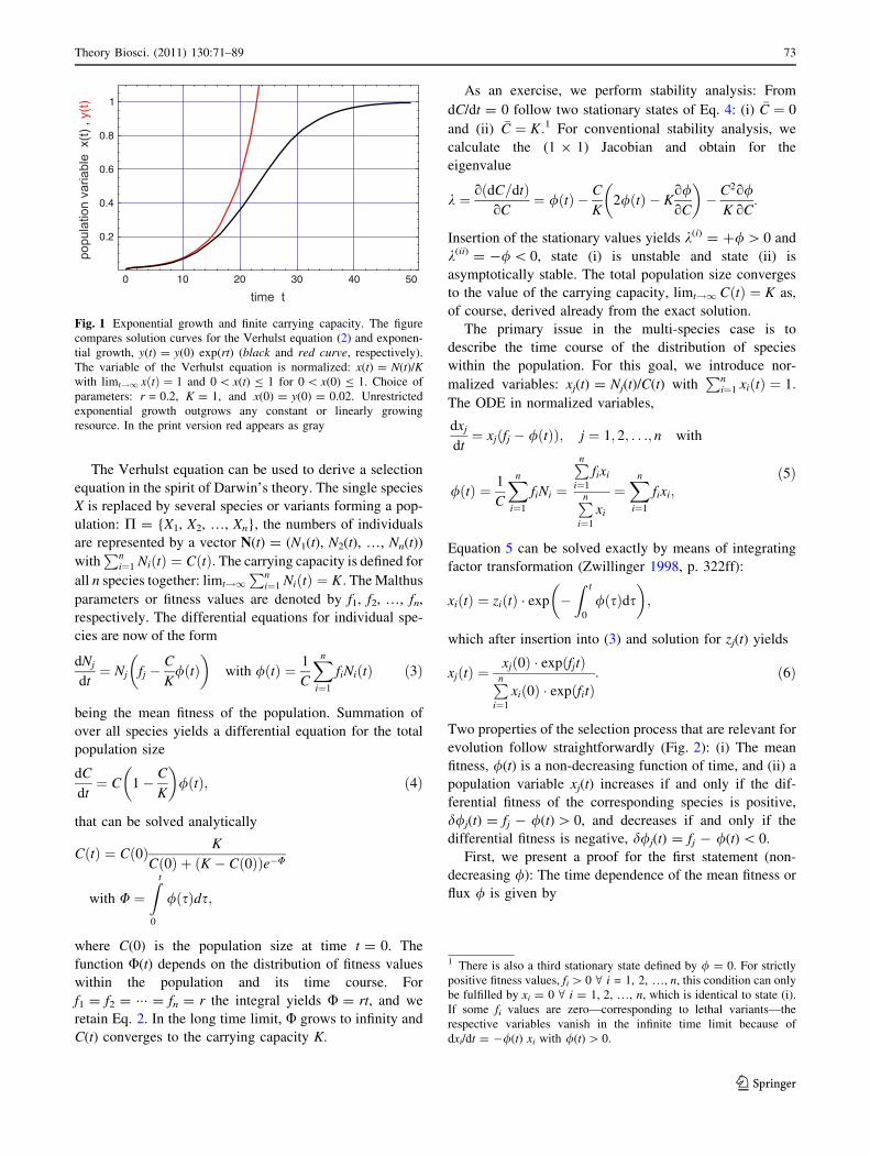
A population of size N(0) grows exponentially at short

times: N(t) & N(0) exp(rt) for N(0) � K at t sufficiently

small. As shown in Fig. 1, the population size approaches

the carrying capacity asymptotically for long times:

limt!1 NðtÞ ¼ K:

The two parameters are taken as criteria to distinguish

different evolutionary strategies: Species that are r-selected

exploit ecological niches with low density, produce a large

number of offspring each of which has a low probability to

survive to adulthood, whereas K-selected species are

strongly competing in crowded niches and invest heavily in

few offspring that have a high probability to survive to

adulthood. The two cases, r- and K-selection, are the

extreme situations of a continuum of mixed selection

strategies. In the real world, the r-selection strategy is an

appropriate adaptation to fast changing environments,

whereas K-selection pays in slowly varying or constant

environments.

72 Theory Biosci. (2011) 130:71–89

123

The Verhulst equation can be used to derive a selection

equation in the spirit of Darwin’s theory. The single species

X is replaced by several species or variants forming a pop-

ulation: P = {X1, X2, …, Xn}, the numbers of individuals

are represented by a vector N(t) = (N1(t), N2(t), …, Nn(t))

withPn

i¼1 NiðtÞ ¼ CðtÞ: The carrying capacity is defined for

all n species together: limt!1Pn

i¼1 NiðtÞ ¼ K: The Malthus

parameters or fitness values are denoted by f1, f2, …, fn,

respectively. The differential equations for individual spe-

cies are now of the form

dNj

dt¼ Nj fj �

C

K/ðtÞ

� �with /ðtÞ ¼ 1

C

Xn

i¼1

fiNiðtÞ ð3Þ

being the mean fitness of the population. Summation of

over all species yields a differential equation for the total

population size

dC

dt¼ C 1� C

K

� �/ðtÞ; ð4Þ

that can be solved analytically

CðtÞ ¼ Cð0Þ K

Cð0Þ þ ðK � Cð0ÞÞe�U

with U ¼Z t

0

/ðsÞds;

where C(0) is the population size at time t = 0. The

function U(t) depends on the distribution of fitness values

within the population and its time course. For

f1 = f2 = ��� = fn = r the integral yields U = rt, and we

retain Eq. 2. In the long time limit, U grows to infinity and

C(t) converges to the carrying capacity K.

As an exercise, we perform stability analysis: From

dC/dt = 0 follow two stationary states of Eq. 4: (i) �C ¼ 0

and (ii) �C ¼ K:1 For conventional stability analysis, we

calculate the (1 9 1) Jacobian and obtain for the

eigenvalue

k ¼ oðdC=dtÞoC

¼ /ðtÞ � C

K2/ðtÞ � K

o/oC

� �� C2

K

o/oC:

Insertion of the stationary values yields k(i) = ?/ [ 0 and

k(ii) = -/\ 0, state (i) is unstable and state (ii) is

asymptotically stable. The total population size converges

to the value of the carrying capacity, limt!1 CðtÞ ¼ K as,

of course, derived already from the exact solution.

The primary issue in the multi-species case is to

describe the time course of the distribution of species

within the population. For this goal, we introduce nor-

malized variables: xj(t) = Nj(t)/C(t) withPn

i¼1 xiðtÞ ¼ 1:

The ODE in normalized variables,

dxj

dt¼ xjðfj � /ðtÞÞ; j ¼ 1; 2; . . .; n with

/ðtÞ ¼ 1

C

Xn

i¼1

fiNi ¼

Pni¼1

fixi

Pni¼1

xi

¼Xn

i¼1

fixi;ð5Þ

Equation 5 can be solved exactly by means of integrating

factor transformation (Zwillinger 1998, p. 322ff):

xiðtÞ ¼ ziðtÞ � exp �Z t

0

/ðsÞds

� �;

which after insertion into (3) and solution for zj(t) yields

xjðtÞ ¼xjð0Þ � expðfjtÞPn

i¼1

xið0Þ � expðfitÞ: ð6Þ

Two properties of the selection process that are relevant for

evolution follow straightforwardly (Fig. 2): (i) The mean

fitness, /(t) is a non-decreasing function of time, and (ii) a

population variable xj(t) increases if and only if the dif-

ferential fitness of the corresponding species is positive,

d/j(t) = fj - /(t) [ 0, and decreases if and only if the

differential fitness is negative, d/j(t) = fj - /(t) \ 0.

First, we present a proof for the first statement (non-

decreasing /): The time dependence of the mean fitness or

flux / is given by

Fig. 1 Exponential growth and finite carrying capacity. The figure

compares solution curves for the Verhulst equation (2) and exponen-

tial growth, y(t) = y(0) exp(rt) (black and red curve, respectively).

The variable of the Verhulst equation is normalized: x(t) = N(t)/Kwith limt!1 xðtÞ ¼ 1 and 0 \ x(t) B 1 for 0 \ x(0) B 1. Choice of

parameters: r = 0.2, K = 1, and x(0) = y(0) = 0.02. Unrestricted

exponential growth outgrows any constant or linearly growing

resource. In the print version red appears as gray

1 There is also a third stationary state defined by / = 0. For strictly

positive fitness values, fi [ 0 V i = 1, 2, …, n, this condition can only

be fulfilled by xi = 0 V i = 1, 2, …, n, which is identical to state (i).

If some fi values are zero—corresponding to lethal variants—the

respective variables vanish in the infinite time limit because of

dxi/dt = -/(t) xi with /(t) [ 0.

Theory Biosci. (2011) 130:71–89 73

123

d/dt¼Xn

i¼1

fi _xi ¼Xn

i¼1

fi fixi � xi

Xn

j¼1

fjxj

!

¼Xn

i¼1

f 2i xi �

Xn

i¼1

fixi

Xn

j¼1

fjxj ¼ f 2 � f� �2¼ varffg� 0:

ð7Þ

Since a variance is always nonnegative, Eq. 7 implies that

/(t) is a non-decreasing function of time, and hence it is

optimized during selection. h

The second statement (differential fitness d/j) is trivial

but provides insight into the selection mechanism. At t = 0

all population variables with a fitness below average, i.e.,

with a negative differential fitness, d/\ 0, will decrease,

all variables with d/[ 0 will increase. The result is an

increase in /(t) in agreement with Eq. 7. As time pro-

gresses and /(t) increases, more and more species fall

under the d/\ 0-criterion, will decrease and finally dis-

appear. Ultimately, only the species with the largest fitness

value, Xm : fm ¼ maxff1; f2; . . .; fng; will remain and the

mean fitness has reached its maximal value: /(t) = fm.

Selection of the fittest has occurred!

The Augustinian monk Gregor Mendel was a contem-

porary of Charles Darwin and had the missing piece of

Darwin’s theory, a mechanism of inheritance (Mendel

1866, 1870) in hand, but his works were ignored by evo-

lutionary biologists until the turn of the century. The

English statistician and geneticist Ronald Fisher succeeded

in uniting natural selection with Mendelian genetics (Fisher

1930). His selection equation describes the evolution of the

distribution of alleles at a single gene locus:

dxj

dt¼Xn

i¼1

ajixixj � xj/ðtÞ ¼ xj

Xn

i¼1

ajixi � /ðtÞ !

¼ xj�fj � /ðtÞ� �

; with �fj ¼Xn

i¼1

ajifi; j ¼ 1; 2; . . .; n

and /ðtÞ ¼Xn

j¼1

Xn

i¼1

ajixixj: ð8Þ

The variables denote the frequencies of the alleles in the

population xj = [Xj], normalization yieldsPn

j¼1 xj ¼ 1;

and aij is the fitness of the (diploid) genotype XiXj. A

diploid organisms carries two alleles of each gene on a

autosome2—one being transferred from the father and one

coming from the mother—and the contribution to the

change of the frequency of allele Xj in time is proportional

to the fitness of the genotype, aij, and the frequencies of the

two alleles, xi and xj. In conventional genetics the proper-

ties of a phenotype are assumed to be independent of the

origin of alleles—it does not matter whether the alleles

comes form the father or from the mother—and therefore,

we have aji = aij (Fig. 3): The matrix of fitness values

A = {aij} is symmetric. In this case, it is straightforward to

prove that /(t), the mean fitness of the alleles is a non-

decreasing function of time as shown for the simple

selection case analyzed in Eq. 7.

In contrast to the simple selection case (3), Fisher’s

selection equation may have several asymptotically stable

stationary states and therefore the outcome of selection

depends on initial conditions. A straightforward example is

provided by higher fitness of the homozygote genotypes

compared to the heterozygote: the states corresponding to the

homozygotes X1X1 and X2X2 (x1 = 1, x2 = 0 and x1 = 0,

x2 = 1, respectively) are asymptotically stable whereas

the heterozygous states X1X2 and X2X1 (x1 = x2 =

0.5) is unstable.3 Unfortunately—but fortunately for

Fig. 2 Differential fitness and selection. In the upper part of the figure,

we show the time development of a population at constant population

size, C = K = 1. The three species differ in initial presence and fitness

values: X1, x1(0) = 0.759, f1 = 0.99 (yellow); X2, x2(0) = 0.240,

f2 = 1.00 (green); X3, x3(0) = 0.001, f3 = 1.01 (red). The lower partof the figure compares differential fitness of individual species, d/j; j =

1, 2, 3 (yellow, green, and red; left ordinate scale), and the mean fitness

of the population, /(t) (black; right ordinate scale). The population

variable of a species increases if the differential fitness is positive and

decreases for negative differential fitness (as follows directly from a

comparison of the two plots). The mean fitness is a non-decreasing

function of time. In the print version red appears as the darkest gray and

other colors differ in their gray-value

2 All chromosomes are autosomes except the sexual chromosomes X

and Y.3 In case matrix A is not symmetric, the dynamical system (10) may

show more complex dynamics like oscillations, deterministic chaos,

etc.

74 Theory Biosci. (2011) 130:71–89

123

population geneticists and theoretical biologists because it

provided and provides a whole plethora of problems to

solve—Fisher’s selection equation holds only for indepen-

dent genes. Two and more locus models with gene interac-

tion turned out to be much more complicated and no

generally valid optimization principle has been found so far:

Natural selection in the sense of Charles Darwin is an

extremely powerful optimization heuristic but no theorem.

Nevertheless, Fisher’s fundamental theorem is much deeper

than the toy version that has been presented here. The

interested reader is referred to a few, more or less arbitrarily

chosen references from the enormous literature on this issue

(Price 1972; Edwards 1994; Okasha 2008).

Mutation driven evolution of molecules

Molecular biology was born when Watson and Crick

published their centennial paper on the structure of DNA.

Further development provided information on the chemis-

try of life at a breathtaking pace (Judson 1979). A closer

look on the structure of DNA revealed the discrete nature

of base pairing—two nucleotides make a base pair that fits

into the double helix or they do not. With this restriction,

the natural nucleobases allow only for four combinations:

AU, UA, GC, and CG. This fact is sufficient for an

understanding of the molecular basis of genetics: genetic

information is of digital nature and multiplication of

information is tantamount to copying. Mutation, the pro-

cess that leads to innovation in evolution, was disclosed as

imperfect reproduction or an error in the copying process.

Correct reproduction and mutation at the molecular level

are seen as parallel chemical reactions (figure 4). In order

to guarantee inheritance, correct copying must occur more

frequently than mutation (as indicated in the figure cap-

tion). In ‘‘The kinetic model of replication and mutation’’

section, we shall cast this intuitive statement into a quan-

titative expression, whereby for the sake of simplicity only

point mutations will be considered. This, however, should

not mean that other changes in genomes like insertions,

deletions, duplications, and other genome rearrangements

are unimportant.

The more general a model is, the wider is its range of

applicability. The enormous success of Darwin’s natural

selection is its almost universal applicability and this

results from the lack of specific assumptions on the process

of multiplication and variation. On the other hand, speci-

ficity is required for working out mathematical models,

which can provide explanation for observations and which

are suitable for experimental test. DNA replication is an

extremely complicated process involving some twenty

proteins,4 and has not yet been studied thoroughly by

biochemical kinetics. Compared to DNA replication, rep-

lication of RNA viruses, in particular bacteriophages, is

rather simple in the sense that it usually requires only a

single enzyme. Since the mechanism of replication has

been resolved down to molecular details in few systems

only, we describe here replication by the specific replicase

from the bacteriophage Qb (Biebricher and Eigen 1988;

Eigen and Biebricher 1988; Nakaishi et al 2002; Hosoda

et al 2007) as an illustration of complete bottom-up

understanding of evolution in vitro.

Virus-specific RNA replication

Qb-replicase is a virus-specific, RNA-dependent RNA

polymerase and amplifies suitable RNA molecules in a

medium containing the activated nucleotides, ATP, UTP,

GTP, and CTP, in excess (Mills et al 1967). in early

experiments Qb-replicase was isolated from Escherichia

coli bacteria infected by Qb bacteriophage, at present

production of the enzyme makes use of genetic engineer-

ing.5 Replication of Qb-RNA is initiated by a single strand

RNA molecule that binds to the enzyme Qb-replicase at

sequence specific recognition sites (Brown and Gold 1996;

Kuppers and Sumper 1975). Through enzyme action, the

X2

X1X1

X1

X1

X2

X1

X1

X2

X2X1

X2

X2

X2

X1

X2

diploid haploid diploid

a11

a12 = a21

a22

Fig. 3 Mendelian genetics and sexual reproduction. In sexual

reproduction the two copies of a gene X in a diploid organism are

separated to yield two haploid gametes. In the offspring the two genes

in the two gametes are combined at random resulting in recombina-

tion. The figure sketches the progeny of two heterozygous organ-

isms—these are organisms carrying two different alleles of the gene.

The fitness of the diploid phenotype, Xi Xj, is denoted by aij

4 Protein synthesis in vivo is regulated by a complex network

controlling gene activity called gene expression. The network

involves regulation of transcription (DNA ? RNA), post-transcrip-

tional modification and maturation of the messenger-RNA, its

translation into protein, and post-translational modification before

the protein unfolds its function.5 Qb-replicase is an enzyme consisting of four subunits. Three

subunits are host proteins involved in translation, the ribosomal

protein S1 and the elongation factors Ef-Tu and Ef-Ts. The fourth

subunit is a virus-specific protein encoded by the viral RNA.

Theory Biosci. (2011) 130:71–89 75

123

template strand is completed—nucleotide after nucleotide

in the direction from the 30- to the 50-end—and forms

locally a double-helical RNA duplex. The process of rep-

lication follows a simple principle making use of strand

complementarity and is often denoted as complementary

replication: Like in the historical silver-based photography,

the plus strand acts as template for the synthesis of the

minus strand, and vice versa, the minus strand is the

template for plus strand synthesis. In vivo and in vitro,

Qb-replicase plays a twofold role: (i) It increases the

accuracy of replication by reinforcing correct base pairing

(A=U and G:C) and (ii) it assists separation of the two

complementary strands—template and newly synthesized

RNA molecule—in the RNA duplex into individual strands

during replication (Mills et al 1967; Weissmann 1974).

Strand separation is essential for successful replication,

because dissociation of the complete RNA duplex is ther-

modynamically so unfavorable that it does not occur at the

temperature applied for replication.6 In Qb RNA replica-

tion, the whole length RNA duplex helix is never formed

since the double helical stretch needed for template poly-

merization is separated into a plus and a mins strand on the

fly (Fig. 5), both strands form their energetically favored

specific single strand structures and prevent duplex for-

mation. In this context it is worth mentioning that an

enzyme-free experiment of cross-catalytic reproduction of

RNA molecules with rich single strand structure has been

successful (Lincoln and Joyce 2009).

Complementary replication is as efficient for population

growth as direct replication is: after internal stationarity

has been achieved, the plus–minus ensemble grows like a

single unit of reproduction. Under the conditions of a

closed system (no exchange of materials with the envi-

ronment, see Fig. 6) RNA replication passes three phases

of growth: exponential growth, linear growth, and satura-

tion (Biebricher et al. 1983, 1984, 1985). Selection and

Darwinian evolution require exponential growth and

accordingly, an open system is indispensable in order to

maintain replication within the exponential phase (Phil-

lipson and Schuster 2009, chaps. 2, 3) by means of a flow.

The easiest way to achieve this goal is to supply all

materials consumed in RNA synthesis by a constant influx

and to remove RNA in excess by an outflux that, in

addition, compensates also for the increase in volume

caused by the influx. The relatively low accuracy of viral

RNA replication (see section: ‘‘The error threshold of

reproduction’’) produces a sufficiently rich variety of

variants that provide the basis for in vitro evolution

(Joyce 2007).

The kinetic model of replication and mutation

The kinetic reaction mechanism of RNA replication in

vitro has been studied in great detail (Biebricher et al.

1983, 1984, 1985): Under suitable conditions, excess rep-

licase and nucleotide triphosphates (ATP, UTP, GTP, and

CTP), the concentration of the RNA plus–minus ensemble

grows exponentially (Fig. 6). The population maintains

exponential growth when the consumed material is

replenished either by a suitable flow device or serial

transfer of small quantities of the reaction mixture into

fresh medium (Spiegelman 1971). Under these conditions,

replication kinetics can be simplified and properly descri-

bed by the differential equation:

+

+

+

+

M

+

+ +

+

+

+

+

M M

XjXj

Xj

X2

X1

Xj

Xn

Xj

Xj

Xj

Xj

Q1j

Q2j

Qjj

Qnj

fjk+j

k j

Fig. 4 A molecular view of replication and mutation. The replicase

molecule (violet) binds the template RNA molecule (Xj, orange) with a

binding constant Kj = k?j/k-j and replicates with a rate parameter fj.The reaction leads to a correct copy with frequency Qjj and to a mutant

Xk with frequency Qkj with Qjj � Qkj V k = j. Stoichiometry of

replication requiresPn

i¼1 Qij ¼ 1; since the product has to be either

correct or incorrect. The sum of all activated monomers is denoted by M.

In the print version the mutant spectrum differs in the gray-value from

lightest for X1 to darkest for Xn

6 Standard amplification of single stranded DNA by means of the

polymerase chain reaction (PCR) is a frequently used technique for

replication that circumvents isothermal duplex dissociation by means

of a temperature program: Single stranded DNA is completed to a

double helical duplex by means of a polymerase from Thermophilusaquaticus (Taq), the duplex is dissociated into single stands at

higher temperature, and cooling of single strands completes the cycle

(see also Cahill et al. 1991).

76 Theory Biosci. (2011) 130:71–89

123

dxj

dt¼Xn

i¼1

Qjifixi � /ðtÞxj; j ¼ 1; 2; . . .; n with /ðtÞ

¼Xn

i¼1

fixi or in vector notationdx

dt¼ Q � F� /ðtÞð Þx;

ð9Þ

where x is an n-dimensional column vector; Q and F are

n 9 n matrices. The matrix Q contains the mutation

probabilities—Qji referring to the production of Xj as an

error copy of template Xi—and F is a diagonal matrix whose

elements are the replication rate parameters or fitness values

fi (Fig. 4). Equation 9 can be transformed into a linear ODE

by means of integrating factor transformation and than

solved by means of an eigenvalue problem (Thompson and

McBride 1974; Jones et al. 1976):

zðtÞ ¼ xðtÞ � exp

Z t

0

/ðsÞds

0@

1A;

dz

dt¼ Q � Fz ¼Wz and W ¼ B � K � B�1 or

K ¼ B�1 �W � B;

with K being a diagonal matrix containing the eigenvalues

of W, k0, k1, …, kn-1. Whenever a path of consecutive

single point mutations can be found from every Xi to every

Xj the matrix W is primitive7 and fulfils Perron–Frobenius

theorem (Seneta 1981, pp. 3, 22). Accordingly, the largest

eigenvalue, k0, is strictly positive and non-degenerate and

the corresponding right hand eigenvector f0 has only

positive entries. The calculation of the solutions xj is

somewhat lengthy but straightforward:

xjðtÞ ¼

Pn�1

k¼0

bjk

Pni¼1

hkixið0Þ expðkktÞ

Pnl¼1

Pn�1

k¼0

blk

Pni¼1

hkixið0Þ expðkktÞ; j ¼ 1; 2; . . .; n:

ð10Þ

The new quantities in this equation are the elements of the

two transformation matrices:

B ¼ fbjk; j ¼ 1; 2; . . .; n; k ¼ 0; 1; . . .; n� 1g and

B�1 ¼ fhkj; k ¼ 0; 1; . . .; n� 1; j ¼ 1; 2; . . .; ng

The columns of B and the rows of B-1 represent the right

hand and left hand eigenvectors of the matrix W. For

example, we have

f0 ¼

b10

b20

..

.

bn0

0BBB@

1CCCA:

5'

3'

5'

Adenine Uracil

CytosineGuanine

Fig. 5 Sketch of RNA

replication by Qb-replicase. An

RNA template—here the plus-

strand of the SV11 variant of

Qb-RNA (Biebicher and Luc,

1992)—is bound to the replicase

and replication proceeds by

adding single activated

nucleotides one after the other

to the growing product, the

minus strand. The replicase

operates on single stranded

stretches. Double helical

structural elements on the

template strand are opened

when they are encountered by

the enzyme. Still on the enzyme,

the duplex formed during

replication is separated in order

to allow for independent

structure formation of both

strands

7 A square non-negative matrix T = {tij; i, j = 1, …, n; tij C 0} is

called primitive if there exists a positive integer m such that Tm is

Footnote 7 continued

strictly positive: Tm[0 which implies Tm = {tij(m); i, j = 1, …, n; tij

(m)[0}.

Theory Biosci. (2011) 130:71–89 77

123

Since k0 [ k1 C k2 ��� C kn-1, the stationary solution

contains only the contributions of the largest eigenvector,

f0 :

limt!1

xjðtÞ ¼ �xj ¼bj0

Pni¼1

h0ixið0Þ

Pnl¼1

bl0

Pni¼1

h0ixið0Þ; j ¼ 1; 2; . . .; n: ð11Þ

In other words, f0 describes the stationary distribution of

mutants and represents the genetic reservoir of an asexually

reproducing species similarly to the gene pool of a sexual

species. For this reason, f0 has been called quasi-species.

The error threshold of reproduction

The dependence of quasi-species on the frequency of

mutation is considered in this subsection. In general, the

mutation rate is not tunable, but it can be varied within

certain limits in suitable experimental assays. In order to

illustrate, mutation rate dependence and to subject it to

mathematical analysis, a simplifying model assumption

called uniform error rate model is made (Eigen 1971).

The error rate per nucleotide and replication, p, is assumed

to be independent of the position and the nature of the

nucleotide exchange (for example, A ? U, A ? G or

A ? C occur with the same frequency p and the total error

rate at a given position is 3p). Then the elements of the

mutation matrix Q depend only on three quantities: the

chain length of the sequence to be replicated, ‘, the error

frequency p, and the Hamming distance between the tem-

plate, Xi, and the newly synthesized sequence, Xj, denoted

by dijH,8

Qji ¼ 1� ðj� 1Þpð Þ‘�dHij �pdH

ij ¼ ð1� ðj� 1ÞpÞ‘edHij

with e ¼ p

1� ðj� 1Þp:ð12Þ

The size of the nucleotide alphabet is denoted by j—for

natural polynucleotides we have j = 4 corresponding to

{A, U(T),G,C}. The explanation of the two terms in Eq. 12

is straightforward: The two sequences differ in dijH positions

and hence ‘ - dijH nucleotides have to be copied correctly,

each contributing a factor 1 - (j - 1)p, and dijH errors

with frequency p have to be made at certain positions.

Since the Hamming distance is a metric, we have dijH = dji

H,

and within the approximation of the uniform error rate

model, the mutation matrix Q is symmetric.

For p = 0, we encounter the selection case (6): in

absence of degeneracy—all fitness values fj are different—

the species of highest fitness, the master sequence Xm, is

selected and all other variants disappear in the long time

limit. The other extreme is random replication, a condition

under which all single nucleotide incorporations, correct or

incorrect, namely A ? A, A ? U, A ? G, and A ? C,

are equally probable and occur with frequency ~p ¼ 0:25:

Generalization from four to j letters is straightforward:

Then, for ~p ¼ j�1 all elements of matrix Q are equal to j-‘

where ‘ is again the sequence length. If all sequences are

considered in the model the matrix W contains n = j‘

identical rows and takes on the following form at p ¼ ~p

~W ¼ j�‘

f1 f2 . . . fn

f1 f2 . . . fn

..

. ... . .

. ...

f1 f2 . . . fn

0BBB@

1CCCA:

The uniform distribution P ¼ f�xj ¼ n�18 j ¼ 1; 2; . . .;

n with n ¼ j‘g is the eigenvector corresponding to the

largest eigenvalue k0 ¼ j�‘Pn

i¼1 fi; whereas all all other

eigenvalues of W vanish.9 In the whole range 0 B p B j-1,

the stationary distribution changes from the homogeneous

Fig. 6 Kinetics of RNA replication in closed systems. The time

course of RNA replication by Qb-replicase shows three distinct

growth phases: (i) an exponential phase, (ii) a linear phase, and (iii) a

phase characterized by saturation through product inhibition

(Biebricher et al. 1983, 1984, 1985). The experiment is initiated by

transfer of a very small sample of RNA suitable for replication into a

medium containing Qb-replicase and the activated monomers, ATP,UTP, GTP, and CTP in excess (consumed materials are not

replenished in this experiment). In the phase of exponential growth,

there is shortage of RNA templates, every free RNA molecule is

instantaneously bound to an enzyme molecule and replicated, and the

corresponding over-all kinetics follows dx/dt = f�x resulting in

x(t) = x0 � exp(ft). In the linear phase, the concentration of template

is exceeding that of enzyme, every enzyme molecule in engaged in

replication, and over-all kinetics is described by dx/dt = k0 � e0(E) = k,

wherein e0(E) is the total enzyme concentration, and this yields after

integration x(t) = x0 ? kt. Further increase in RNA concentration

slows down the dissociation of product (and template) RNA from the

enzyme–RNA complex and leads to a phenomenon known as product

inhibition of the reaction. At the end, all enzyme molecules are

blocked by RNA in complexes and no more RNA synthesis is

possible, c(t) ? c?

8 The Hamming distance dijH between two strings, Xi and Xj of equal

length counts the number of positions in which the two end-to-end

aligned strings differ (Hamming 1986).9 It can be proven by means of a recursion that the eigenvalues of the

matrix ~W fulfill the relation kn�1 k� j�‘Pn

i¼1 fi� �

¼ 0:

78 Theory Biosci. (2011) 130:71–89

123

population, Nm ¼ f�xm ¼ 1; �xj ¼ 08j 6¼ mg to the uniform

distribution P: A remark concerning the uniform distribu-

tion is required: the number of possible polynucleotide

sequences -j‘ = 4‘ for natural molecules—exceeds by far

any accessible population size already for small RNAs with

‘ & 30. Although Eq. 10 predicts the uniform distribution

in theory, no stationary population is possible in practice, and

we expect populations to drift randomly through sequence

space (Derrida and Peliti 1991; Huynen et al. 1996; and

‘‘Modeling evolution in silico’’ section). A limitation of

modeling by differential equations is encountered [see also

the localization threshold of mutant distributions (McCaskill

1984; Eigen et al. 1989)].

Between the two extremes, the function �xmðpÞ was

approximated by Manfred Eigen through neglect of back-

flow from mutants to the master sequence. He obtained for

dxm/dt = 0 (Eigen 1971):

�xm ¼ Qmm ��f�m

fm¼ Qmm � r�1

m with �f�m ¼

Pni¼1;i 6¼m

fi�xi

1� �xm:

ð13Þ

The quantity rm ¼ fm=�f�m is denoted as the superiority of

the master sequence. In this rough, zeroth order

approximation, the frequency of the master sequence

becomes zero at a critical value of the mutation rate

parameter, pmax, for constant chain length ‘ or at a maximal

chain length ‘max for constant replication accuracy p,

pmax �ln rm

ðj� 1Þ‘ or ‘max �ln rm

ðj� 1Þp;

respectively. The critical replication accuracy has been

characterized as error threshold of replication. As we shall

see in the ‘‘Fitness landscapes and error thresholds’’ sec-

tion, the error threshold reminds of a phase transition in

which the quasi-species changes from a mutant distribution

centered around a master sequence to some other distri-

bution that is only weakly dependent on p or independent at

all, for example the uniform distribution.10 In other words,

the solution that becomes exact at p ¼ ~p is closely

approached at p = pmax already. For the purpose of illus-

tration for a superiority of rm = 1.1 and a chain length of

‘ = 100, we obtain pmax = 0.00032 compared to ~p ¼ 0:25:

Both relations for the error threshold, maximum replica-

tion accuracy and maximum chain length, were found to

have practical implications: (i) RNA viruses replicate at

mutation rates close to the maximal value (Drake 1993). A

novel concept for the development of antiviral drugs makes

use of this fact and aims at driving the virus population to

mutation rates above the error threshold (Domingo 2005).

(ii) There is a limit in chain length for faithful replication that

depends on the replication machinery: the accuracy limit of

enzyme-free replication is around one error in one hundred

nucleotides, RNA viruses with a single enzyme and no proof

reading can hardly exceed accuracies of one error in 10,000

nucleotides, and DNA replication with repair on the fly

reaches one error in 108 nucleotides. For prokaryotic DNA

replication, post-replication repair increases the accuracy to

10-9–10-10, which is roughly one mutation in 300 dupli-

cations of bacterial cells (Drake et al. 1998).

Fitness landscapes and error thresholds

The approximation of the error threshold through neglect

of mutational back-flow (13) caused the results to be

independent of the distribution of replication parameters of

mutants, since only the mean replication rate, �f�m; enters

the expression. As a matter of fact, the appearance of an

error threshold and its shape depend on the fitness land-

scape (Wiehe 1997; Phillipson and Schuster 2009,

pp. 51–60). In this subsection we shall now consider the

influence of the distribution of fitness values in two steps:

(i) different fitness values are applied for sequences with

different Hamming distances from the master sequence,

and (ii) different fitness values are assigned to individual

sequences. In the first case, all sequences Xj with Hamming

distance dm,jH = k fall into the error class k. Although the

assumption that all sequences in a given error class have

identical fitness is not well justified on the basis of

molecular data, it turns out to be useful for an under-

standing of the threshold phenomenon.

The following five model landscapes or fitness matrices

F = {Fij = fi � dij} were applied (Fig. 7): (i) the single-peak

landscape corresponding to a mean field approximation, (ii)

the hyperbolic landscape, (iii) the step-linear landscape,

(iv) the multiplicative landscape, and (v) the additive or

linear landscape. Examples for the dependence of the

quasi-species distribution on the error rate are shown in

Fig. 8.

For analyzing error thresholds, it is useful to consider

three separable features: (i) the decay in the frequency of

the master sequence—xm(p) ? 0 in the zeroth order

approximation (13), (ii) the phase transition-like sharp

change in the mutant distribution, and (iii) the transition

from the quasi-species to the uniform distribution. All the

three phenomena coincide on the single-peak landscape

(Fig. 8; upper part). Characteristic for most hyperbolic

landscapes is an abrupt transition in the distribution of

sequences according to (ii) but—in contrast to the single-

peak landscape—the transition does not lead to the uniform

10 A sharp transition from the structured quasi-species to the uniform

distribution is found for the single-peak landscape and some related

landscapes only (see ‘‘Fitness landscapes and error thresholds’’

section.

Theory Biosci. (2011) 130:71–89 79

123

distribution, instead another distribution is formed that

changes gradually into the uniform distribution, which

becomes the exact solution at the point p ¼ ~p: The step-

linear landscape illustrates the separation of the decay

range (i) and the phase transition to the uniform distribu-

tion (ii and iii). In particular, variation in the position of the

step (‘c’ in Fig. 7) that the phase transition point pmax shifts

towards higher values of p when the position of the step

moves towards higher error-classes, whereas the decrease

in the decay of the master sequence moves in opposite

direction. The additive and the multiplicative landscape,

the two landscapes that are often used in population

genetics, do not sustain threshold-behavior. On these two

landscapes, the quasi-species is transformed smoothly with

increasing p into the uniform distribution.

Error thresholds on realistic fitness landscapes can be

modeled straightforwardly by the assumption of a scattered

distribution of fitness values within a given band of width

d for all sequences except the master sequence11:

f ðXjÞ ¼ �f�m þ d grndðjÞ � 0:5ð Þ � 1;

j ¼ 1; 2; . . .; j‘; j 6¼ m:ð14Þ

In this expression ’grnd(j)’ is a random number drawn from

some random number generator with a uniform distribution

of numbers in the range 0 B grnd(j) B 1 with j being the

index of the consecutive calls of the random function and

d is the band width of fitness values. Similarly the uniform

error rate model (12) is only a rough approximation to the

distribution of mutation frequencies. In order to relax the

stringent constraint here, we define a local mutation rate pk

for each position k (k = 1, 2, …, ‘) along the sequence and

assume again that the individual pk values vary within a

given band width. The computational capacities of today

allow for studies of error thresholds at the resolution of

individual sequences up to chain lengths n = 10. Further

increase in computational power raises expectation to be

able to reach n = 20, which in case of binary sequences is

tantamount to the diagonalization of 106 9 106 matrices.

Three questions are important in the context of resolu-

tion of fitness values down to individual sequences: (i)

How does the dispersion of fitness values expressed in

terms of the band width d change the characteristics of the

error threshold, (ii) how does variation in local mutation

rates influence error threshold and (iii) what happens if two

more sequences have the same maximal fitness value fm.

The answers to question (i) and (ii) follow readily from the

Fitn

ess

valu

es

()

fX

k

Error class k

dH( , )X Xk 010 10

Fitn

ess

valu

es

()

fX

k

Error class k

dH( , )X Xk 0

10

Fitn

ess

valu

es

()

fX

k

Error class k

dH( , )X Xk 0

c

0 1 5 9 0 1 2 3 4 5 6 7 8 9

0 1 5

2 3 4 6 7 8

2 3 4 6 7 8 9 0 1 2 3 4 5 6 7 8 9 10

Fitn

ess

valu

es

()

fX

k

Error class k

dH( , )X Xk 0

Fig. 7 Some examples of model fitness landscapes. The figure shows

five model landscapes with identical fitness values for all sequences in

a given error class: (i) the single peak landscape (f(X0) = f0 and

f(Xj) = fn V j = 1, …, n; upper left drawing), (ii) the hyperbolic

landscape (f(Xj) = f0 - (f0 - fn)(n ? 1)j/(n(j ? 1)) Vj = 0, …, n; upperright drawing, black curve), (iii) the step-linear landscape (f(Xj) = f0

- (f0 - fn)j/k V j = 0, …, k and f(Xj) = fn V j = k ? 1, …, n; lower leftdrawing), (iv) the multiplicative landscape (f(Xj) = f0 (fn/f0)j/n Vj =

0, …, n; upper right drawing, red curve), and (v) the additive or

linear landscape (f(Xj) = f0 - (f0 - fn)j/n V j = 0, …, n; lower rightdrawing). In the print version red appears as gray

11 The data obtained from biomolecules suggest a high degree of

ruggedness for the landscapes derived for structures and functions:

nearby sequences may lead to identical or very different structures.

By the same token functions like fitness values may be the same or

very different for close by lying genotypes. Ruggedness is an intrinsic

property of mapping from biopolymer sequences into structures or

functions.

80 Theory Biosci. (2011) 130:71–89

123

calculated results: the position at which the frequency of

the master sequence in the population reaches a given small

value migrates towards smaller f-values with increasing

band width d. This observation agrees fully with expecta-

tion because the fitness value closest to fm becomes larger

for broader bands of fitness values. The scatter of fitness

values at the same time broadens the transition. Relaxation

of the uniform error rate assumption causes smoothing of

the error threshold and a shift of pmax towards higher values

of p.

Degeneracy of fitness values implies that two or more

genotypes have the same fitness and this is commonly

denoted as neutrality in biology. An investigation of the

role of neutrality requires an extension of Eq. 14. A certain

fraction of sequences, expressed by the degree of neutrality

k, is assumed to have the highest fitness value f0, and the

fitness values of the remaining fraction 1 - k are assigned

as in the non-neutral case (14). This random choice of

neutral sequences together with a random dispersion of the

other fitness values yields an interesting result: random

selection in the sense of Motoo Kimura’s neutral theory of

evolution (Kimura 1983) occurs only for sufficiently dis-

tant fittest sequences. In full agreement with the exact

result derived for the limit p ? 0 (Schuster and Swetina

Fig. 8 Error thresholds on different model fitness landscapes.

Relative stationary concentrations of entire error classes �ykðpÞ ðk ¼0; 1; . . .; ‘; �yk ¼

Pni¼1;dH ðXi ;XmÞ¼k �xiÞ are plotted as functions of the

mutation rate p (the different error classes are color coded, dH(Xi,Xm)

= 0, black; dH(Xi,Xm) = 1, red; dH(Xi,Xm) = 2, yellow,

dH(Xi,Xm) = 3, chartreuse; dH(Xi,Xm) = 4, green, etc). The pictures

at the top show the threshold behavior on the single-peak fitness

landscape (enlarged on the right hand side) where the three conditions

(i), (ii), and (iii)—decay of master, phase transition, and transition to

uniform distribution—coincide. The two pictures in the middle were

computed for the hyperbolic landscape (enlarged on the right hand

side) where the phase transition leads to a distribution that changes

gradually into the uniform distribution and (i) has a slight offset to the

left of (ii). The left-hand figure at the bottom corresponds to the step-

linear landscape and fulfils (ii) and (iii) whereas (i) has a large offset

to the left, and eventually the additive landscape (bottom, right-handside) does not sustain an error threshold at all. Parameters used in the

calculations: ‘ = 100, fm = f0 = 10, fn = 1 (except the hyperbolic

landscape where we used fn = 0.9091 in order to have �f�m ¼ 1 as for

the single peak landscape), and c = 5 for the step-linear landscape. In

the print version red appears as the darkest gray and other colors

differ in their gray-value

Theory Biosci. (2011) 130:71–89 81

123

1988) we find that two fittest sequences of Hamming dis-

tance dH = 1, two nearest neighbors in sequence space, are

selected as a strongly coupled pair with equal frequency of

both members. Numerical results demonstrate that this

strong coupling occurs not only for small mutation rates,

but extends over the whole range of p values from p = 0 to

the error threshold p = pmax. For clusters of more than two

Hamming distance one sequences, the frequencies of the

individual members of the cluster are obtained from the

largest eigenvector of the adjacency matrix. Pairs of fittest

sequences with Hamming distance dH = 2, i.e., two next

nearest neighbors with two sequences in between, are also

selected together but the ratio of the two frequencies is

different from one. Again coupling extends from zero

mutation rates up to the error threshold p = pmax. Strong

coupling of fittest sequences manifests itself in virology as

systematic deviations from consensus sequences of popu-

lations as is indeed observed in nature. For fittest sequences

with dH C 3 random selection chooses one sequence

arbitrarily and eliminates all others as predicted by the

Kimura’s neutral theory of evolution.

Mapping sequences into structures

Modeling evolution of molecules by means of chemical

kinetics solves one vital problem of the theory of evolution:

fitness can be determined independently of the evolution-

ary process by measuring the rate parameters of replication

and the sometimes raised argument that survival of the

fittest is nothing but a tautology, because there is no other

way to measure fitness except running evolution, is obso-

lete. A full understanding of evolution, however, is con-

fronted with enormous complexity even in the simple case

of nucleic acid molecules in the test tube. How does the

fitness of a molecule change in response to mutation? This

question is tantamount to asking for the prediction of

molecular function from known biopolymer sequences,

which is a notoriously hard problem. Commonly prediction

of function is addressed in two steps: (i) prediction of

structure from known sequence and (ii) prediction of

function from known structure. Both tasks are hard in

general and useful solutions are available for special cases

only. An exception are RNA structures on the level of so-

called secondary structures: Structure prediction is acces-

sible by mathematical and computational methods

(Schuster 2006). The discreteness of nucleotide interac-

tions—either two nucleotides form a base pair or they do

not—facilitates the analysis of RNA structures and allows

for the application of efficient dynamic programming

algorithms to structure prediction (Hofacker et al. 1994a;

Zuker and Stiegler, 1981; Zuker, 1989a, b). The relation

between structure and function can be modeled straight-

forwardly for a number of special cases. One example, is

binding between RNA molecules called RNA hybridization

(Hofacker et al. 1994b; Dimitrov and Zuker 2004).

The basic principle of folding RNA sequences into

secondary structures is double helix formation, in essence

the same as used in nucleic acid replication: the single

stranded molecule folds back onto itself when the sequence

allows for (partial) duplex formation (Fig. 9) whereby the

driving force is lowering Gibbs free energy. Since base

pairing logic applies as well to structure formation as to

replication, secondary structures are objects that can be

analyzed by means of combinatorics. Simple logic on one

hand side is counteracted by complexity originating from

nonlocal interactions. As illustrated in the example of

Fig. 9 distant nucleotides as well close by lying ones may

form base pairs. The full three-dimensional structure of

RNA molecules is built through forming additional

nucleotide interactions called tertiary interactions, which

are often stabilized by divalent cations, especially by

Mg2�: Tertiary interactions are either sequence specific

and can be catalogued therefore (Leontis et al. 2006) or

they follow a general principle like, for example, ’end-on-

end’ stacking of helices from secondary structure (Moore

1999).

Because of the discreteness of RNA structure space,

mappings from RNA sequence space into structure space

can be addressed by combinatorics and have been studied

extensively (Fontana et al 1993; Schuster et al. 1994;

Reidys et al. 1997; Fontana and Schuster 1998b; Stadler

et al. 2001). Six properties of these mappings appear to be

relevant for evolution (Schuster 2006):

(i) The numbers of RNA sequences exceed by far the

numbers of RNA secondary structures and neutrality

with respect to structures is inevitable.

(ii) Sequences folding into the same structure form

neutral networks that are the pre-images of structures

in sequence space.

(iii) Depending on the degree of neutrality, neutral

networks are either connected or split into compo-

nents. The critical connectivity threshold depends

only on the number of letters in the nucleotide

alphabet.

(iv) Neutral networks in the conventional {A,U,G,C} -

space are larger and more likely to be connected than

neutral networks in the binary or {G,C}-space.

(v) Neutral networks are embedded in sets of sequences

that are compatible with the structure.12

(vi) The intersection of the compatible sets of two

structures is always non-empty. In other words, for

12 Compatibility means that the sequence can form the structure but

not necessarily as the minimum free energy structure.

82 Theory Biosci. (2011) 130:71–89

123

two given structures it is always possible to find a

sequence that can form both.

Evidence for the existence and strong hints on the

properties of neutral networks come from RNA selection

experiments (Schultes and Bartel 2000; Held et al. 2003;

Huang and Szostak 2003). For a more complete under-

standing of neutrality in evolution of molecules further

development of the theory and appropriate experiments are

needed.

Modeling evolution in silico

Stochasticity is essential for evolution—each mutant after

all starts out from a single copy and random drift in the

sense of Motoo Kimura is a pure stochastic phenomenon. A

large number of studies have been conducted on stochastic

effects in population genetics (Blythe and McKane 2007).

Not too much work, however, has been done so far on the

development of a general stochastic theory of molecular

evolution. We mention two examples representative for

others (Jones and Leung 1981; Demetrius et al. 1985). In

the latter case, the reaction network for replication and

mutation was analyzed as a multi-type branching process,

and it was proven that the stochastic process converges to

the solutions of the deterministic Eq. 9 in the limit of large

populations.

In order to simulate the interplay between mutation

acting on the RNA sequence and selection operating on

RNA structures, the sequence-structure map has to be

turned into an integral part of the model (Fontana and

Schuster 1987; Fontana et al. 1989; Fontana and Schuster

1998b): The sequence is the genotype and the RNA sec-

ondary structure represents the phenotype. The simulation

tool starts from a population of RNA molecules and sim-

ulates chemical reactions corresponding to replication and

mutation in a continuous stirred flow reactor (CSTR) by

using Gillespie’s algorithm (Gillespie 1976, 1977, 2007).

Fitness parameters are predefined functions of RNA

structures—Eq. 15 presents an example. Molecules repli-

cate in the reactor and produce correct copies and mutants

according to a stochastic version of the mechanism shown

in Fig. 4, the material consumed is supplied by a contin-

uous influx of stock solution into the reactor, and excess

material is removed by means of an outflux compensating

the increase in volume. Whenever a new sequence is pro-

duced by mutation, the corresponding structure and its

fitness are calculated. The stochastic process in the reactor

is constructed to have two absorbing states: (i) extinction—

all RNA molecules are diluted out of the reaction vessel,

Fig. 9 The secondary structure of a typical transfer RNA. The

nucleotide sequence folds back on itself through forming double

helical stacks whenever sequence complementarity allows for it (lefthand sketch; individual stacks are color coded). In the symbolicnotation, a secondary structure is represented by an equivalent string

with parentheses and dots whereby each single nucleotide is

represented by a dot, each base pair by a parenthesis, and mathemat-

ical notation applies (string at the bottom of the figure). The

secondary structure is converted into the full three-dimensional

structure by forming additional stabilizing interactions between

nucleotides (right hand sketch). One general principle in tertiary

structure formation is extension of helices through ’end-on-end’

stacking: The green helix extends the red one, and the violet helix

extends the blue one in the figure above. The molecular example

shown is the phenylalanyl-transfer RNA (tRNAphe) from the yeast

Saccharomyces cerevisiae. The letters D, M, Y, T,and P denote

modified nucleotides

Theory Biosci. (2011) 130:71–89 83

123

and (ii) success—the reactor has produced the predefined

target structure. The population size determines the out-

come of the computer experiment: Below N = 18 the

reactor goes into extinction with a probability greater 0.5

and it reaches the target with a high probability close to one

for population sizes N [ 20. For sufficiently large popu-

lations the probability of extinction is very small, for

population sizes reported here, N C 1000, extinction has

been never observed.

In target search problems the replication rate of a

sequence Xk, representing its fitness fk, is chosen to be a

function of the Hamming distance between the symbolic

notations of the structure formed by the sequence,

Sk = f(Xk) and the target structure ST,

fkðSk; STÞ ¼1

aþ dHðSk; STÞ=‘: ð15Þ

An adjustable parameter a is introduced in order to avoid

infinite fitness when the target is reached (here it was chosen

to be 0.1). The fitness increases when Sk approaches the

target, a trajectory is completed when the population reaches

a sequence that folds into the target structure. A typical

trajectory is shown in Fig. 10. In this simulation a homog-

enous population consisting of N molecules with the same

random sequence and the corresponding structure is chosen

as initial condition. The target structure was chosen to be the

well-known secondary structure of phenylalanyl-transfer

RNA (tRNA phe) shown in Fig. 9. The mean distance to

target of the population decreases in steps until the target is

reached (Fontana et al. 1989; Fontana and Schuster 1998a, b;

Schuster 2003). Individual (short) adaptive phases are

interrupted by long quasi-stationary epochs.

Optimization dynamics in phenotype space is recon-

structed in terms of a time ordered series of structures that

leads from an initial structure SI to the target structure ST.

This series, called the relay series, is a uniquely defined and

uninterrupted sequence of structures in the flow reactor. It is

retrieved through backtracking, that is in opposite direction

from the final structure to the initial structure: the procedure

starts by highlighting the final structure and traces it back

during its uninterrupted presence in the flow reactor until the

time of its first appearance. At this point, we search for the

parent structure from which it descended by mutation. Now,

we record time and structure, highlight the parent structure,

and repeat the procedure. Recording further backwards

yields a series of structures and times of first appearance,

which ultimately ends in the initial population.13 Usage of

the relay series and its theoretical background allows for

classification of transitions (Fontana and Schuster 1998a;

Stadler et al. 2001): Minor or frequent transitions occur

almost instantaneously, they are manifested by small chan-

ges in the structures commonly involving one or two base

pairs, and major or rare transitions, which require random

drift in neutral subspaces in order to find an appropriate

starting point for the successful mutation. Major transition

are accompanied by larger structural changes (Fontana and

Schuster 1998a; and Fig. 11).

Inspection of the relay series together with the sequence

record on the quasi-stationary plateaus provides an expla-

nation for the stepwise approach towards the target and

allows for a distinction of two scenarios:

(i) The structure is constant and we observe neutral

evolution in the sense of Kimura’s theory of neutral

Fig. 10 A trajectory of evolutionary optimization. The topmost plot

presents the mean distance to the target structure of a population of

1000 molecules. The plot in the middle shows the width of the

population in Hamming distance between sequences and the plot at

the bottom is a measure of the velocity with which the center of the

population migrates through sequence space. Diffusion on neutral

networks causes spreading on the population in the sense of neutral

evolution Huynen et al (1996). A remarkable synchronization is

observed: At the end of each quasi-stationary plateau a new adaptive

phase in the approach towards the target is initiated, which is

accompanied by a drastic reduction in the population width and a

jump in the population center (the top of the peak at the end of the

second long plateau is marked by a black arrow). A mutation rate of

p = 0.001 was chosen, the replication rate parameter is defined in Eq.

15, and initial as well as target structure are shown in Table 1

13 It is important to stress two facts about relay series: (i) The same

shape may appear two or more times in a given relay series series.

Then, it was extinct between two consecutive appearances. (ii) A

relay series is not a genealogy which is the full recording of parent-

offspring relations a time-ordered series of genotypes.

84 Theory Biosci. (2011) 130:71–89

123

evolution (Kimura 1983). In particular, the numbers of

neutral mutations accumulated are proportional to the

number of replications in the population, and the

evolution of the population can be understood as a

diffusion process on the corresponding neutral net-

work (Huynen et al. 1996, see also Fig. 10).

(ii) The process during the stationary epoch involves

several structures with identical replication rates and

the relay series reveal a kind of random walk in the

space of these neutral structures.

The diffusion of the population on the neutral network is

illustrated by the plot in the middle of Fig. 10 that shows

the width of the population as a function of time (Schuster

2003). The population width increases during the quasi-

stationary epoch and sharpens almost instantaneously after

a sequence had been produced that allows for the start of a

new adaptive phase in the optimization process. The sce-

nario at the end of the plateau corresponds to a bottle neck

of evolution. The lower part of the figure shows a plot of

the migration rate or drift of the population center and

Fig. 11 The relay series of an

in silico evolution experiment.

The relay series consists of 44

steps leading from the initial

structure SI = S0 to the target

structure ST = S44. Lower caseroman letters (a, b, c,… )

indicate major transitions and

lower case Greek letters (a, b, c…) identify closely related

structures. The backgroundcolor indicates stretches of

closely related structures in the

relay series. It is worth noticing

that the same structures can

appear several times in the relay

series (e.g., shapes 19–30). The

construction of relay series is

described in the text. The figure

is taken from Fontana and

Schuster (1998a, suppl. 1)

Theory Biosci. (2011) 130:71–89 85

123

confirms this interpretation: On the plateaus the drift is

very slow but becomes fast at the end of the plateau when

the population center moves quickly or ‘jumps’ in

sequence space from one point to another point from where

a new adaptive phase can be initiated (as manifested by the

peaks in Fig. 10). A closer look at the figure reveals the

coincidence of the three events: (i) collapse-like narrowing

of the population spread, (ii) jump-like migration of the

population center, and (iii) beginning of a new adaptive

phase.

It is worth mentioning that the optimization behavior

observed in a long-term evolution experiment with Esch-

erichia coli (Lenski et al. 1991) can be readily interpreted

in terms of random searches on a neutral network. Starting

with twelve colonies in 1988, Lenski and his coworkers

observed after 31,500 generation or 20 years, a great

adaptive innovation in one colony (Blount et al. 2008).

This colony developed a kind of membrane channel that

allows for uptake of citrate, which is used as buffer in the

medium. The colony thus conquered a food source that led

to a substantial increase in colonial growth. The mutation

leading to citrate import into the cell is reproducible with

earlier isolates of this particular colony that has apparently

traveled on the neutral network to a position from where

the adaptive mutation is within reach. All other eleven

colonies did not give rise to mutations with similar func-

tion. The experiment is a nice demonstration of contin-

gency in evolution: the conquest of the citrate resource

does not happen through a single highly improbable

mutation but by means of a mutation with standard prob-

ability from a particular region of sequence space where

the population had traveled in one case out of twelve—

history matters, or repeating Theodosius Dobzhansky’s

(1977) famous quote: ‘‘Nothing makes sense in biology

except in the light of evolution’’.

Table 1 collects some numerical data harvested by

sampling of evolutionary trajectories under identical con-

ditions.14 Individual trajectories show enormous scatter in

the time or in the number of replications required to reach

the target. The mean values and the standard deviations

were obtained from statistics of trajectories under the

assumption of log-normal distributions. Despite the scatter,

three features are unambiguously detectable:

(i) The search in GC sequence space takes about five

times as long as the corresponding process in AUGC

sequence space in agreement with the difference in

neutral network structure (Schuster, 2003, 2006).

(ii) The time to target decreases with increasing popula-

tion size.

(iii) The number of replications required to reach target

increases with population size.

Combining items (ii) and (iii) allows for a clear con-

clusion concerning time and material requirements of the

optimization process: fast optimization requires large

populations whereas economic use of material suggests to

work with small population sizes just sufficiently large to

avoid extinction.

A simulation study on the parameter dependence of in

silico RNA evolution has been reported recently (Kupczok

and Dittrich 2006). Increase in mutation rate leads to an

error threshold phenomenon that is closely related to the

one observed with quasi-species on a single-peak landscape

as described above (Eigen et al. 1989). Evolutionary opti-

mization becomes more efficient15 with increasing error

rates until the error threshold is reached. Further increase in

the error rate leads to an abrupt breakdown of the optimi-

zation process. As expected, the distribution of replication

rates or fitness values fj in sequence space is highly relevant

too: steep decrease of fitness with the distance to the master

structure—represented by the target that has the highest

fitness value—leads to sharp threshold behavior reminding

of a single-peak landscape, whereas flat landscapes show

broad maxima of optimization efficiency without an indi-

cation of a threshold-like behavior.

Concluding remarks

The exceedingly complex phenomenon of evolution takes

place on multiple organizational levels, which range from

cell organelles and cells to organs, organisms and popu-

lations. All these levels are different manifestations of the

phenotype. A comprehensive description is not yet at hand

and mathematical modeling as well as experimental studies

inevitably have to concentrate on individual aspects or

modules of the system. Nevertheless, the reductionists’

program to partition the whole into tractable subsystems

and to reconstitute it with the detailed knowledge of a

lower level of description turned out to be impressively

successful. In case of the cell, for example, molecular

biology has first reduced the highly complex entity to

individual biomolecules—nucleic acids, proteins, carbo-

hydrates, lipids and others—and subjected the parts to

biochemical and biophysical analysis. Next followed the

study of the supramolecular complexes, molecular

machines, and organelles within the cell. Starting with

genomics and proteomics in the nineteen nineties and

14 Identical means here that everything was kept unchanged in the

computer experiments except the seeds for the random number

generator.

15 Efficiency of evolutionary optimization is measured by average

and best fitness values obtained in populations after a predefined

number of generations.

86 Theory Biosci. (2011) 130:71–89

123

continuing with systems biology at the turn of the century

the object of investigation at the molecular level has been

shifted from single molecules to higher units, cells, organs,

and eventually organisms. The goal of the new biology is

to complete the bottom-up approach from chemistry and

physics and to provide a novel access to the understanding

of the complexity of life as well as to develop new tools

and techniques for the exploration of biology specific

phenomena. Still there is a long way to go before this goal

will be reached and the unsolved problems exceed by far

the available solutions, but the contours of a new and

comprehensive theoretical biology that is rooted in math-

ematics, physics, and chemistry are already apparent.

Evolution of molecules, viruses, and bacteria is studied

under simplified conditions in vitro and in silico, and, in

principle, allows for the incorporation of molecular

mechanisms of reproduction, mutation, and recombination

into the equations of the evolutionary process. Chemical

kinetics of virus specific RNA replication is well under-

stood and even in this very simple case the process or

reproduction is quite complicated. Modeling DNA repli-

cation kinetics at full molecular resolution is still a great

challenge but solvable by means of the current experi-

mental techniques. If replication is already so complicated,

how can the Darwinian theory of variation and selection be

fairly simple and work? The answer is straightforward:

Only the numbers of individuals, parents and progeny, are

counted and the internal structure of the replicating entities,

molecules, cells, organisms or societies, plays no role.

Moreover replication in nature does never operate under

conditions of excess of nucleic acids, because cellular

division controls the number of genetic information carri-

ers. Virus reproduction in the host cell is the only well

known counterexample: Replication continues until the

available resources are exhausted. Genetics like natural

selection was discovered on a completely empirical basis.

No explanations were at hand, neither for the observations

nor for the deviations from the idealized ratios. In the

second half of the twentieth century, an understanding of

the Mendelian rules was provided by the molecular

approach to heredity and at the same time a natural

explanation was given for the deviations from them. Epi-

genetics was invoked as a deus ex machina in order to

explain phenomena that escaped explanations by genetics.

Recently, most of these previously strange observations

found a straightforward explanation on the molecular level.

Modeling evolution by differential equations is well

established and—although not yet available—a compre-

hensive stochastic approach will complement conventional

modeling. Computer simulation of chemical kinetics of

evolution is still in an early state and the simulations are

lacking a more systematic approach. One still unsolved

problem concerns the parameter space for molecular

properties. A true wealth of data is currently obtained in

genomics and related disciplines but only some of them

will be useful for modeling evolution. The problem is how

to find the pearls in a mess of rubbish. A second major

limitation comes from the hyper-astronomical size of

sequence space containing j‘ different genotypes. At

present, all genotypes can be considered routinely for short

Table 1 Statistics of the optimization trajectories

Alphabet Population size Number of runs Real time from start to target Number of replications [107]

N nR Mean value r Mean value r

AUGC 1000 120 900 ?1380 -542 1.2 ?3.1-0.9

2000 120 530 ?880-330 1.4 ?3.6 -1.0

3000 1199 400 ?670 -250 1.6 ?4.4 -1.2

10000 120 190 ?230 -100 2.3 ?5.3 -1.6

30000 63 110 ?97 -52 3.6 ?6.7 -2.3

100000 18 62 ?50 -28 – –

GC 1000 46 5160 ?15700 -3890 – –

3000 278 1910 ?5180 -1460 7.4 ?35.8 -6.1

10000 40 560 ?1620 -420 – –

The table shows the results of sampled evolutionary trajectories leading from a random initial structure SI to the structure of tRNAphe, ST as

target. Simulations were performed with an algorithm introduced by Gillespie (1976, 1977, 2007). The time unit is here undefined and real timeimplies proportionality to real measurements of time. A mutation rate of p = 0.001 per site and replication was used. The mean and standard

deviation were calculated under the assumption if a log-normal distribution that fits the data of the simulations. For less than 50 runs, no statistics

is given for the number of replication because the uncertainty is too large

The structures SI and ST were used in the optimization:

SI: ((.(((((((((((((............(((....)))......)))))).))))))).))...(((......)))

ST: ((((((...((((........)))).(((((.......))))).....(((((.......))))).))))))....

Theory Biosci. (2011) 130:71–89 87

123

chain lengths up to ‘ = 10. Extension to ‘ = 20 provides

already a challenge to numerical methods even for binary

sequences, since the number of genotype interactions

reaches a magnitude of 106 9 106. Nature itself provides

the solution: Whole sequence spaces are never covered,

clones are confined to tiny parts of the space and drift

slowly by the mechanisms of evolution. The enormous size

of sequence space, on the other hand, provides a con-

vincing explanation for the existence of bacterial species:

Their genomes are so far apart in sequence space that they

do not require reproductive isolation. Despite steady

migration they won’t meet and merge.

The real complexity in biology arises from genotype–

phenotype relations. Simple model landscapes are used in

population genetics but they are far from being realistic and

lead to wrong predictions. Even in the simplest case of in

vitro evolution of molecules, the genotype–phenotype map

requires understanding of the folding of biopolymer

sequences into structures and the derivation of function from

structure. This understanding as well as the predictive power

of theories and algorithms in this field is still poor. Never-

theless, a few hints can be derived already from these simple

model systems. Mappings involving biopolymers are com-

monly rugged, and optimization on rugged landscapes is an

especially hard problem, because search strategies including

the evolutionary approach involving populations are trapped

very likely in some minor local optimum. The solution is

obvious from the properties of biopolymers: nearby

sequences may give rise to entirely different structures and

functions but very often they lead to phenotypes that are

indistinguishable by selection or neutral. Biological land-

scapes are not only rugged they are also characterized by a

fairly high degree of neutrality. Sequence space is high-

dimensional and this implies the existence of a large number

of independent directions—commonly denoted as orthogo-

nal. If the population during an adaptive walk in one direc-

tion is caught in a local optimum, there is a good chance that

an escape from the trap is possible in some other direction

where neutral sequences are found. A landscape structured in

this way—ruggedness accompanied by a sufficiently high

degree of neutrality—enables stepwise optimization: Short

adaptive phases are supplemented by long quasi-stationary

periods of random drift on neutral networks. At the same

time the optimization process receives a memory on its past:

Because of the high dimensionality of sequence space,

individual trajectories are unique in the long run. A popu-

lation migrating along a path collects series of stochastic

events, which are not repeatable. Short term migration of

populations, however, can be reproduced and this leads to an

interesting kind of biological contingency: the recent past is

repeatable whereas developments taking long time and col-

lecting long series of mutations are not. Although the

underlying dynamics is very different, the physicist will be

reminded a little bit of irreversibility in thermodynamics.

References

Biebicher CK, Luce R (1992) In vitro recombination and terminal

elongation of RNA by Qb replicase. EMBO J 11(13):5129–5135

Biebricher C, Eigen M (1988) Kinetics of RNA replication by Qbreplicase. In: Domingo E, Holland J, Ahlquist P (eds) RNA

genetics, vol I. CRC Press, Boca Raton, pp. 1–21

Biebricher CK, Eigen M, William C, Gardiner J (1983) Kinetics of

RNA replication. Biochemistry 22:2544–2559

Biebricher CK, Eigen M, William C, Gardiner J (1984) Kinetics of

RNA replication: plus-minus asymmetry and double-strand

formation. Biochemistry 23:3186–3194

Biebricher CK, Eigen M, William C, Gardiner J (1985) Kinetics of

RNA replication:competition and selection among self-replicat-

ing RNA species. Biochemistry 24:6550–6560

Blount ZD, Z C, Lenski RE (2008) Historical contingency an the

evolution of a key innovation in an experimental population of

Escherichia coli. Proc Natl Acad Sci USA 105:7898–7906

Blythe RA, McKane A (2007) Stochastic models of evolution in

genetice, ecology and linguistics. J Stat Mech P07018:1–58

Brown D, Gold L (1996) RNA replication by Qb replicase: a working

model. Proc Natl Acad Sci USA 93:11558–11562

Cahill P, Foster K, Mahan DE (1991) Polymerase chain reaction and

Qb replicase amplification. Clin Chem 37:1482–1485

Darwin C (1859) On the origin of species by means of natural

selection or the preservation of favoured races in the struggle for

life. John Murray, London

Demetrius L, Schuster P, Sigmund K (1985) Polynucleotide evolution

and branching processes. Bull Math Biol 47:239–262

Derrida B, Peliti L (1991) Evolution in a flat fittness landscape. Bull

Math Biol 53:355–382

Dimitrov RA, Zuker M (2004) Prediction of hybridization and

melting for double-stranded nucleic acids. Biophys J 87:215–226

Dobzhansky T, Ayala FJ, Stebbins GL, Valentine JW (1977)

Evolution. W. H. Freeman & Co., San Francisco

Domingo E (ed) (2005) Virus entry into error catastrophe as a new

antiviral strategy. Virus Res 107(2):115–228

Drake JW (1993) Rates of spontaneous mutation among RNA viruses.

Proc Natl Acad Sci USA 90:4171–4175

Drake JW, Charlesworth B, Charlesworth D, Crow JF (1998) Rates of

spontaneous mutation. Genetics 148:1667–1686

Edwards AW (1994) The fundamental theroem of natural selection.

Biol Rev 69:443–474

Eigen M (1971) Selforganization of matter and the evolution of

biological macromolecules. Naturwissenschaften 58:465–523

Eigen M, Biebricher C (1988) Sequence space and quasispecies

distribution. In: Domingo E, Holland J, Ahlquist P (eds) RNA

Genetics, vol III, CRC Press, Boca Raton, pp 211–245

Eigen M, McCaskill J, Schuster P (1989) The molecular quasispecies.

Adv Chem Phys 75:149–263

Fisher RA (1930) The genetical theory of natural selection. Oxford

University Press, Oxford

Fontana W, Schuster P (1987) A computer model of evolutionary

optimization. Biophys Chem 26:123–147

Fontana W, Schuster P (1998a) Continuity in evolution: on the nature

of transitions. Science 280:1451–1455

Fontana W, Schuster P (1998b) Shaping space. The possible and the

attainable in RNA genotype-phenotype mapping. J Theor Biol

194:491–515

88 Theory Biosci. (2011) 130:71–89

123

Fontana W, Schnabl W, Schuster P (1989) Physical aspects of

evolutionary optimization and adaptation. Phys Rev A 40:

3301–3321

Fontana W, Konings DAM, Stadler PF, Schuster P (1993) Statistics of

RNA secondary structures. Biopolymers 33:1389–1404

Gillespie DT (1976) A general method for numerically simulating the

stochastic time evolution of coupled chemical reactions. J Comp

Phys 22:403–434

Gillespie DT (1977) Exact stochastic simulation of coupled chemical

reactions. J Phys Chem 81:2340–2361

Gillespie DT (2007) Stochastic simulation of chemical kinetics. Annu

Rev Phys Chem 58:35–55

Hamming RW (1986) Coding and information theory, 2nd edn.

Prentice-Hall, Englewood Cliffs

Held DM, Greathouse ST, Agrawal A, Burke DH (2003) Evolutionary

landscapes for the acquisition of new ligand recognition by RNA

aptamers. J Mol Evol 57:299–308

Hofacker IL, Fontana W, Stadler PF, Bonhoeffer LS, Tacker M,

Schuster P (1994a) Fast folding and comparison of RNA

secondary structures. Monatshefte fur Chemie 125:167–188

Hofacker IL, Fontana W, Stadler PF, Bonhoeffer LS, Tacker M,

Schuster P (1994b) Vienna RNA package. Current Version 1.8.4.

Institute for Theoretical Chemistry, University of Vienna,

Vienna.

Hosoda K, Matsuura T, Kita H, Ichihashi N, Tsukada K, Yomo T

(2007) Kinetic analysis of the entire RNA amplification process

by Qb replicase. J Biol Chem 282:15516–15527

Huang Z, Szostak JW (2003) Evolution of aptamers with a new

specificity and new secondary structures from an ATP aptamer.

RNA 9:1456–1463

Huynen MA, Stadler PF, Fontana W (1996) Smoothness within

ruggedness. The role of neutrality in adaptation. Proc Natl Acad

Sci USA 93:397–401

Jones BL, Leung HK (1981) Stochastic analysis of a non-linear model

for selection of biological macromolecules. Bull Math Biol

43:665–680

Jones BL, Enns RH, Rangnekar SS (1976) On the theory of selection

of coupled macromolecular systems. Bull Math Biol 38:15–28

Joyce GF (2007) Forty years of in vitro evolution. Angew Chem Int

Ed 46:6420–6436

Judson H (1979) The eighth day of creation. The makers of the

revolution in biology. Jonathan Cape, London

Kimura M (1983) The neutral theory of molecular evolution.

Cambridge University Press, Cambridge

Kupczok A, Dittrich P (2006) Determinants of simulated RNA

evolution. J Theor Biol 238:726–735

Kuppers B, Sumper M (1975) Minimal requirements for template

recognition by bacteriophage Qb replicase: approach to general

RNA-dependent RNA synthesis. Proc Natl Acad Sci USA

72:2640–2643

Lenski RE, Rose MR, Simpson SC, Tadler SC (1991) Long-term

experimental evolution in Escherichia coli. I. Adaptation and

divergence during 2,000 generations. Am Nat 38:1315–1341

Leontis NB, Lescoute A, Westhof E (2006) The building blocks and

motifs of RNA architecture. Curr Opin Struct Biol 16:279–287

Lincoln TA, Joyce GF (2009) Self-sustained replication of an RNA

enzyme. Science 323:1229–1232

Malthus TR (1798) An Essay of the principle of population as it

affects the future improvement of society. J. Johnson, London

Maxam A, Gilbert W (1977) A new method of sequencing DNA. Proc

Natl Acad Sci USA 74:560–564

McCaskill JS (1984) A localization threshold for macromolecular

quasispecies from continuously distributed replication rates.

J Chem Phys 80:5194–5202

Mendel G (1866) Versuche uber Pflanzen-Hybriden. Verhandlungen

des naturforschenden Vereins in Brunn 4:3–47

Mendel G (1870) Uber einige aus kunstlicher Befruchtung gewonne-

nen Hieracium-Bastarde. Verhandlungen des naturforschenden

Vereins in Brunn 8:26–31

Mills DR, Peterson RL, Spiegelman S (1967) An extracellular

Darwinian experiment with a self-duplicating nucleic acid

molecule. Proc Natl Acad Sci USA 58:217–224

Moore PB (1999) Structural motifs in RNA. Annu Rev Biochem

68:287–300

Nakaishi T, Iio K, Yamamoto K, Urabe I, Yomo T (2002) Kinetic

properties of Qb replicase, an RNA dependent RNA polymerase.

J Biosci Bioeng 93:322–327

Okasha S (2008) Fisher’s fundamental theorem of natural selection—

a philosophical analysis. Br J Phil Sci 59:319–351

Phillipson PE, Schuster P (2009) Modeling by nonlinear differential

equations. Dissipative and conservative processes. World Sci-

entific Series on Nonlinear Science A, vol 69. World Scientific,

Singapore

Price GR (1972) Fisher’s ‘‘fundamental theorem’’ made clear. Annals

of Human Genetics 36:129–140

Reidys C, Stadler PF, Schuster P (1997) Generic properties of

combinatory maps. Neutral networks of RNA secondary struc-

ture. Bull Math Biol 59:339–397

Sanger F, Nicklen S, Coulson A (1977) DNA sequencing with chain-

terminating inhibitors. Proc Natl Acad Sci USA 74:5463–5467

Schultes EA, Bartel DP (2000) One sequence, two ribozymes:

implications for the emergence of new ribozyme folds. Science

289:448–452

Schuster P (2003) Molecular insight into the evolution of phenotypes.

In: Crutchfield JP, Schuster P (eds) Evolutionary dynamics—

exploring the interplay of accident, selection, neutrality, and

function, Oxford University Press, New York, pp 163–215

Schuster P (2006) Prediction of RNA secondary structures: From

theory to models and real molecules. Reports on Progress in

Physics 69:1419–1477

Schuster P, Swetina J (1988) Stationary mutant distribution and

evolutionary optimization. Bull Math Biol 50:635–660

Schuster P, Fontana W, Stadler PF, Hofacker IL (1994) From

sequences to shapes and back: a case study in RNA secondary

structures. Proc R Soc Lond B 255:279–284

Seneta E (1981) Non-negative matrices and Markov chains, 2nd edn.

Springer-Verlag, New York

Spiegelman S (1971) An approach to the experimental analysis of

precellular evolution. Q Rev Biophys 4:213–253

Stadler BRM, Stadler PF, Wagner GP, Fontana W (2001) The

topology of the possible: formal spaces underlying patterns of

evolutionary change. J Theor Biol 213:241–274

Thompson CJ, McBride JL (1974) On Eigen’s theory of the self-

organization of matter and the evolution of biological macro-

molecules. Math Biosci 21:127–142

Verhulst P (1838) Notice sur la loi que la population pursuit dans son

accroisement. Corresp Math Phys 10:113–121

Weissmann C (1974) The making of a phage. FEBS Lett 40:S10–S18

Wiehe T (1997) Model dependency of error thresholds: the role of

fitness functions and contrasts between the finite and infinite sites

models. Genet Res Camb 69:127–136

Zuker M (1989a) On finding all suboptimal foldings of an RNA

molecule. Science 244:48–52

Zuker M (1989b) The use of dynamic programming algorithms in

RNA secondary structure prediction. In: Waterman MS (ed)

Mathematical methods for DNA sequences, CRC Press, Boca

Raton, pp 159–184

Zuker M, Stiegler P (1981) Optimal computer folding of larger RNA

sequences using thermodynamics and auxiliary information.

Nucl Acids Res 9:133–148

Zwillinger D (1998) Handbook of differential equations, 3rd edn.

Academic Press, San Diego

Theory Biosci. (2011) 130:71–89 89

123