mathematical models and statistical methods in molecular ... · week 3 - thurs 27th jan 9.00am -...

Week 3 - Thurs 27th Jan9.00am - 12.00

Mathematical models and statistical methods in molecular biologyJulia Brettschneider

In the last two decades, molecular biology research has made enormous progress. Mathematical models can play a crucial role in describing the complex structure of the new discoveries in this field. The acceleration of the scientific research has been enabled by new high-throughput molecular measurement technologies. The resulting new kinds of high-dimensional data sets require the development of appropriate statistical methods. [...]

This seminar will give an overview of central topics in modern molecular biology and of the role that mathematics and statistics can play in this discipline. It will cover many examples including the discovery of genes linked to certain phenotypes, multiple testing, gene networks, data quality and molecular diagnostics.

Outline

• Part I: Introduction to genomics

• Part II: Natural sciences & mathematical sciences

• Part III: Examples

Part IIntroduction to genomics

1. Basic molecular biology and genomics

2. Applications in biology and medicine

3. Introduction to measurement technologies

Now you are here

Procaryotes

Eucaryotes

Similarities between eucaryotes and procaryotes: cell membrane, DNA

Main differences: true nuclei, hierarchically struct. chromosomes, membrane-bound organelles

Unicelluar eucaryotes: “Protista” (mostly marine organisms)Multicellular eucaryotes: Plants, fungi, animals

http://www.goldiesroom.org/Note%20Packets/03%20Cytology/00%20Cytology--WHOLE.htm

Plant cell Animal cell

a few main differences



Genetic informationChromosomes

DNA (contains genes)

Nucleotide

DNA replication

ACGT:Nucleic acids

Construction of proteins

Proteins are building blocks for cells.

Proteins are built according to genetic information ina multi-step process.

Central Dogma of Molecular Biology

Cell

DNA

RNA

Striated muscle

Cells: same genes,

different looks

..., stone walls, roof, divided into room, glass

windows, wooden frames, hardwood doors,...

Plan

Textual description

Metaphor: Architecture

Product

Design team

Construction

Plan(different)

Textual description

(same)

Process and product are not deterministic

Product(different)

Design team

Construction

..., stone walls, roof, divided into room, glass

windows, wooden frames, hardwood doors,...

Plan

Textual description

Central Dogma of Molecular Biology

Product

Design

ConstructionRNA

DNA

Cell

The rate of a gene’s products is variable.It depends on:

Can you give specific examples?

What?

Gene expression

Examples?


- reaction to heat shock (in yeast)- yeast cell cycle- liver tissue vs. brain tissue- tumor tissue vs. healthy tissue - brain tissues from schizophrenic person vs. control- blood with and w/o drug influence- embryo development - young vs. old

- type and state of the cell - environmental conditions - developmental stage- .....

Gene expression

Examples?

Gene expression

• Transcript (RNA) level

• Protein level


This rate is called gene expression level.It has two components:

- type and state of the cell - environmental conditions - developmental stage- .....

2. Applications

• Functional genetics and genomics

• Biological research

• Complex genetic diseases

• Measure the expression of a gene in different kinds of tissue (e.g., tumor and control)

• Infer if the gene contributes to the phenotypical differences (e.g., plays a role in tumor growth).

Functional genetics

This approach needs candidate genes

Traditional research approach:“Is gene A involved in biological

process xyz?”

Functional genomics

• Understanding cellular processes: e.g., which genes are involved in the yeast cell cycle?

• Etiology of complex genetic diseases: e.g., which genes play a role in schizophrenia?

• Effects of environmental factors (e.g., light, temp.)

Exploratory research approach:“Which genes are involved in

biological process xyz?”

This approach needs new technology

Biology

• Developmental processes

• Circadian clock

• Cell cycle

• Reaction to stimulus (e.g. temperature change, chemical)

Examples of typical areas for gene expression studies:

Complex genetic diseases

• Cancers, brain disorders, cardio-vascular diseases, asthma, some skin diseases, some birth defects, etc. have a genetic component, among other factors

• Detect differentially expressed (patients vs controls) genes and discover pathways

• Test reaction to treatments on molecular level

• Refine disease subtypes

• Tailor treatment type to individual

• Develop diagnostic and prognostic tests based on individual molecular information

Example: Cancer

http://www.genetics.com.au/factsheet/fs11-3.gif



Example: Depression

http://www.mbni.med.umich.edu/mbni/faculty/burmeister/burmeister.html



Who is interested in this?

www.publications.parliament.uk/pa/ld200809/ldselect/.../107i.pdfwww.publications.parliament.uk/pa/ld200809/ldselect/.../107ii.pdf

For example...

http://www.publications.parliament.uk/pa/ld200809/ldselect/.../107i.pdf




3. Measurement technologies

• Basic principle

• Measuring the expression of one gene

• Measuring the expression of many genes (since 1990s)

Basics• Measurement usually refers to a chemical analysis

(assay) that determines the abundance of a certain compound

• Can be qualitative or quantitative

http://thunder.biosci.umbc.edu/classes/biol414/spring2007/files/biolFISH_olgio_hybridization-deep01_01_03.jpg

Assays for DNA: bind unknown pieces in a tissue sample to known pieces using complementary structure



Southern blot

• Invented by Ed Southern (1975)

• Identification of DNA fragments (in a mixture of unknown material) complementary to a known DNA sequence

http://www.pnas.org/content/suppl/2007/04/27/0702836104.DC1/02836Fig5.jpg





http://www.microscopesblog.com/uploaded_images/southern-blot-702630.gif



Southern blot• Invented by Ed Southern (1975)

• Identification of DNA fragments (in a mixture of unknown material) complementary to a known DNA sequence


Southern blot analysis of independent Ura- lacZ- mutants isolated from wild-type and mft1D cells. DNA from yeast transformants carrying mutant pCM184-LAUR plasmids was isolated from overnight cultures in SC and used for Southern analysis by digestion with HindIII, electrophoresis, and hybridization with radiolabeled pCM184-LAUR, or for sequence analysis of different fragments of lacZ and URA3 amplified by PCR.





No joke!

• Northern blot

• Western blot

• Eastern blot

• Far-Eastern blot

• Eastern-Western blotting

• ...

Microarrays• First high-throughput technology for gene expression

measurement (1990s)

• Opened up new avenues of research: functional genomics

• Assay tens of thousands of genes simultaneously in one experiment

• By now: a number of different platforms made by companies such as Agilent and Affymetrix

• Quality has been improving, prices vary accordingly

33

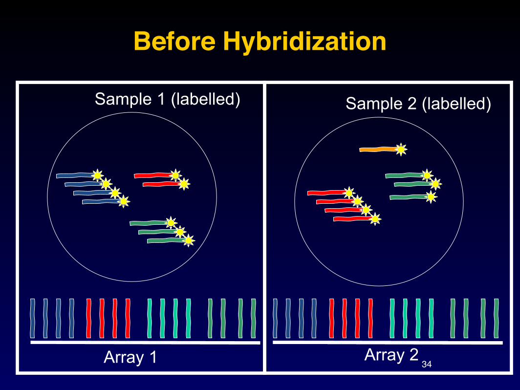
Nucleic acid hybridization: here DNA-RNA

34

Before Hybridization

Array 1 Array 2

Sample 1 (labelled) Sample 2 (labelled)

35

After Hybridization

Array 1 Array 2

4 2 0 3 0 4 0 3

36

Microarray

24µm

Millions of copies of a specificoligonucleotide probe synthesized in situ (“grown”)

Image of Hybridized Probe Array

>200,000 differentcomplementary probes

Single stranded, labeled RNA targetOligonucleotide probe

* **

**

1.28cm

GeneChip Probe ArrayHybridized Probe Cell

Compliments of D. Gerhold

Part IINatural sciences &

mathematical sciences

David Hilbert, 8 September 1930 in Königsberg/KaliningradCongress of the Association of German Natural Scientists and Medical Doctors, Speech “Naturerkennen und Logik”:

The instrument that mediates between theory and practice, between thought and observation, is mathematics; it builds the bridge and makes it stronger and stronger...

math.sfsu.edu/smith/Documents/HilbertRadio/HilbertRadio.pdf


The instrument that mediates between theory and practice, between thought and observation, is mathematics; it builds the bridge and makes it stronger and stronger.

Euler proved that it was not possible to plan a route that would cross each of the seven bridges of Königsberg exactly once, whether or not you ended up in the same place as you began.

http://people.engr.ncsu.edu/mfms/SevenBridges/




The instrument that mediates between theory and practice, between thought and observation, is mathematics; it builds the bridge and makes it stronger and stronger. Thus it happens that our entire present day culture, to the degree that it reflects intellectual achievement and the harnessing of nature, is founded on mathematics. GALILEO said long ago: Only he can understand nature who has learned the language and signs by which it speaks to us; this language is mathematics and its signs are mathematical figures. KANT declared, “I maintain that in each natural science there is only as much true science as there is mathematics.” In fact, we don’t master a theory in natural science until we have extracted its mathematical kernel and laid it completely bare. [...] We must know. We will know.

Establishing knowledgeEpistemiology Stats (concept) Stats (math technique)

Theory A hypothesis Stochastic model

EvidenceMeasurements on

a sample Data

Judgement

Decision based on likelihood of

hypothesis given measurements

Comparison of probabilities for

observing the data in model

Discussion Quality of decision Error rates

Definition: knowledge = true justified belief

Perspective:- empirical- quantitative- non-deterministic

Scientific Method

The scientific method1. Observation

2. Tentative description (hypothesis)

3. Predictions

4. Test by experiment

5. Repeat 3./4. to build theory, i.e. framework for explaining observations and making predictions http://physics.ucr.edu/~wudka/Physics7/Notes_www/node6.html

http://physics.ucr.edu/~wudka/Physics7/Notes_www/node6.html


The scientific method1. Observation

2. Tentative description (hypothesis)

3. Predictions

4. Test by experiment

5. Repeat 3./4. to build theory, i.e. framework for explaining observations and making predictions http://physics.ucr.edu/~wudka/Physics7/

Notes_www/node6.html





The scientific method

- unprejudiced

- reproducible

- falsifiable

How do math and stats get into this picture?

Establishing knowledgeEpistemiology Stat test (concept) Stats (math technique)



a sample Data

Judgement






Establishing knowledgeEpistemiology Stat test (concept) Math technique

Theory A hypothesis H0 (and Ha)


a sampleTest statistics

(function of data)

Judgement



Probabilities for observing the data

under H0, Ha

Discussion Quality of decision Error probabilities

Hypothesis testing paradigm

Epistemiology Stats (concept) Math technique



a sampleTest statistics

(function of data)

Judgement




under H0, Ha


Example: z-test Distributions of test statistics (function of data) under H0 and Ha.Decision rule based on critical value

= probability I reject H0 though it’s true (false positive)= probability I do not reject H0 though Ha is true (false negative)

Massive parallel genomic measurement technologies

• DNA: sequencing

• RNA: qtPCR, microarrays (see below), mRNA-Seq

• Proteins: mass spectronomy, protein arrays

Technologies that can assay large numbers of macromolecules simultaneously in one experiment

Examples:

Sandrine Dudoit Multiple Testing Procedures with Applications to Genomics MCP 2007

Multiple Hypothesis Testing Problems in Genomics

! !

!"# $"# %&'()*+

!"#$%&"'(!')$ !"#$%*#!')$

"#$%#&'(&)

*++#,-./

*.()&,#&0

12/.3)#&/

*&&3040(3&5!673&8(&093&:;<

13./,39=2(+,+

1402>4/+

"09%'0%9#!=9#?('0(3&

;94&+'9(=0!.#@#.+

*.()&,#&0

12/.3)#&/

"09%'0%9#!=9#?('0(3&

1402>4/+

%,)+'(-.)/012*'3'4*56316+7153*+*5631'8(5'9)/

2*'3'4*56316++'(6(*'+19)(676(6

:';6&*6()/0<+;*&'+9)+(=1(&)6(9)+(

>)+'(-.)/

Figure 1: Biomedical and genomic data.

July 6, 2007 c�Copyright 2007, all rights reserved Page 7

New generation of technologies opens up new avenues of scientific research

• Understanding routine cellular processes, e.g. which genes are involved in the yeast cell cycle?

• Etiology of complex genetic diseases, e.g. which genes play a role in schizophrenia?

• Molecular diagnosis, e.g. tumor classification by gene expression signatures

For example:




a sample Data

Judgement






All possible hypotheses




a sample Data

Judgement






All possible hypotheses

Advantage:Unprejudiced

Objection:Hypotheses generated mechanically (lack of scientific prioritisation, burry truth in rubbish)

Hypothesis testing paradigm

Epistemiology Stats (concept) Math technique



a sample Test statistics

Judgement




under H0, Ha


many of these

more theory needed here(see Ex. 1)

Part IIIExamples

• Virus sequence variation & hypothesis testing

• Gene expression measurement technologies & data preprocessing and quality

Virus example: DNA sequence variation and

HIV replication capacity(from Dudoit et al, 2007)

• Phenotype: Severity of disease as reflected by its replication capacity (RC) (see fig)

• Genotype (DNA): Codons/amimo acids in protease (PR) and reverse transcriptase (RT) regions

Question: Is replication capacity related to sequence variation?

HIVHIV live

cycle

Virus example: DNA sequence variation and

HIV replication capacity(from Dudoit et al, 2007)

• Phenotype: Severity of disease as reflected by its replication capacity (RC) (> fig)

• Genotype (DNA): Codons/amimo acids in protease (PT) and reverse transcriptase (RT) regions

Question: Is replication capacity related to sequence variation?

Sandrine Dudoit Multiple Hypothesis Testing, Part III PB HLTH 240D – Spring 2007

HIV-1 Sequence Variation and Viral Replication Capacity

Data. The HIV-1 dataset comprises n = 317 records, linking viral

replication capacity with PR and RT sequence data, from

individuals participating in studies at the San Francisco General

Hospital and the Gladstone Institute of Virology and Immunology.

The data for each of the n = 317 patients consist of the following.

• Y , a continuous replication capacity outcome/phenotype.

• X = (X(m) : m = 1, . . . ,M), an

M = 96 + 186 = 282-dimensional covariate vector of binary

codon genotypes in the PR (pr4–pr99) and RT (rt38–rt223)

HIV-1 regions. Codons are recoded as binary covariates, with

value of 0 corresponding to the wild-type codon, i.e., the most

common codon among the n = 317 patients, and value of 1 for

mutant codons, i.e., all other codons.

March 19, 2007 Page 65

Data (from Segal et al, 2004)

Naive approach• For each of the 282 codons m, test whether RC Y is

associates with X(m).

• For each of the 282 codons m, get rejection or non-rejection, along with error probabilities (significance levels).

• Problem: For each of the 282 codons, you make a wrong decision with a small probability, and that accumulates.

Naive approach• For each of the 282 codons m, test whether RC Y is

associates with X(m).

• For each of the 282 codons m, get rejection or non-rejection, along with error probabilities (significance levels).

• Problem: For each of the 282 codons, you make a wrong decision with a small probability, and these accumulate.

Excursion: Multiple testing

A historical sourceAntoine Augustin Cournot (1801-1877, French philosopher, economist, mathem. game theorist) wrote in 1843:

“... it is clear that nothing limits ... the number of features according to which one can distribute [natural events orsocial facts] into several groups or distinct categories.”

His example: investigating the chance of male birth.

“One could distinguish first of all legitimate birth from those occuring out of wedlock,... one can also classify births according to birth order, according to the age, profession, wealth, or religion of the parents... .”

A historical source (ct.)

“Usually, these attempts through which the experimenter passed don’t leave any traces; the public will only know the results that has been found worth pointing out;

... and as a consequence, someone unfamiliar with the attempts which have led to this result completely lacks a clear rule for deciding whether the result can or can not be attributed to chance.”

Generation of multiple hypothesis via subpopulations.

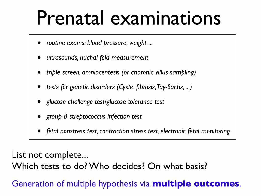
Prenatal examinations• routine exams: blood pressure, weight ...

• ultrasounds, nuchal fold measurement

• triple screen, amniocentesis (or choronic villus sampling)

• tests for genetic disorders (Cystic fibrosis, Tay-Sachs, ...)

• glucose challenge test/glucose tolerance test

• group B streptococcus infection test

• fetal nonstress test, contraction stress test, electronic fetal monitoring

Generation of multiple hypothesis via multiple outcomes.

List not complete... Which tests to do? Who decides? On what basis?

Family-wise error rateDefinition: The family-wise error rate is the probability of at least one FP (i.e., type I error),that is,

The FWER is controlled at level if

FWER ! !

!

FWER = Pr(#FP ! 1)

Compute FWER

FWER = Pr(#FP ! 1)

Let be independent hypotheses. H1,H2, ...,HMAssume the first are true, the others false.m

= 1 ! Pr(#FP = 0)

Pr(#FP = 0) = Pr( not reject H1, ...,Hm)

= (1 ! !1) · . . . · (1 ! !m)where !j = Pr(reject Hj)

FWER = 1 ! !mj=1(1 ! !j)

Ex.: 10 hypothesis, all equal 5%. FWER(m) = 1 ! 0.95m!j

Compute FWER (ct.)Ex.: 10 hypothesis, all equal 5%. FWER(m) = 1 ! 0.95m

FWER(0) = 0%, FWER(1) = 5%, FWER(2) ! 9.8%, FWER(10) ! 40.1%

!j

Traditional “cure”: p-value adjustment

!Want to keep FWER below fixed value

Bonferroni method: Reject any hypothesis with (unadjusted) p-value less or equal to !/M

Adjusted p-values:

Conservative adjustment. More sophisticated methods:Holm (1979) uses order of raw p-values,Westfal & Young’s (1993) step-up and step-down methods use order and joint distribution of raw p-values.

p̃j = min(Mpj , 1)

Controls FWER (proof is straightforward).

Multiple hypothesis in genomics?• Very common

• Number of hypothesis much bigger than in traditional mult. testing ex.

• Ex. virus RC: 282 hypothesis

• Ex. genome-wide study to find disease related genes: tens of thousands of hypothesis

• Traditional adjustment methods not useful

• Traditional concepts of error rates too narrow

Massive multiple testing -new research branch

• Grew quickly, mostly motivated by genomics (but also fMRI, astronomical images)

• Introduction of a variety of concepts for joint error probabilities

• Methods to compute distributions under Null

• New adjustment methods, new concepts

• e.g. Dudoit & van der Laan 2002+


Multiple Hypothesis Testing Framework: Error Rates

Table 1: Type I and Type II errors in multiple hypothesis testing.

Null hypotheses

Non-rejected, Rcn Rejected, Rn

True, H0 Wn = |Rcn ∩H0| Vn = |Rn ∩H0| h0

False, H1 Un = |Rcn ∩H1| Sn = |Rn ∩H1| h1

M −Rn Rn M

Type I errors: Rn ∩H0 Type II errors: Rcn ∩H1




Number of false positives, g(v, r) = v.Generalized family-wise error rate (gFWER):

gFWER(k) = Pr(Vn > k).

Per-family error rate (PFER):

PFER = E[Vn].

Proportion of false positives among the rejected hypotheses, g(v, r) = v/r.Tail probability for the proportion of false positives (TPPFP):

TPPFP (q) = Pr(Vn/Rn > q).

False discovery rate (FDR):

FDR = E[Vn/Rn].

Type I error rates based on the proportion of false positives among the rejected

hypotheses are particularly appealing for large-scale testing problems, as they do

not increase exponentially with the number of tested hypotheses.




Table 1: Type I and Type II errors in multiple hypothesis testing.

Null hypotheses

Non-rejected, Rcn Rejected, Rn

True, H0 Wn = |Rcn ∩H0| Vn = |Rn ∩H0| h0

False, H1 Un = |Rcn ∩H1| Sn = |Rn ∩H1| h1

M −Rn Rn M

Type I errors: Rn ∩H0 Type II errors: Rcn ∩H1




Number of false positives, g(v, r) = v.Generalized family-wise error rate (gFWER):

gFWER(k) = Pr(Vn > k).

Per-family error rate (PFER):

PFER = E[Vn].

Proportion of false positives among the rejected hypotheses, g(v, r) = v/r.Tail probability for the proportion of false positives (TPPFP):

TPPFP (q) = Pr(Vn/Rn > q).

False discovery rate (FDR):

FDR = E[Vn/Rn].

Type I error rates based on the proportion of false positives among the rejected

hypotheses are particularly appealing for large-scale testing problems, as they do

not increase exponentially with the number of tested hypotheses.


and more...

Return to virus ex.Sandrine Dudoit Multiple Hypothesis Testing, Part III PB HLTH 240D – Spring 2007


0 50 100 150 200 250

0.0

0.2

0.4

0.6

0.8

1.0

HIV: M=282 Codon Positions.

Number of rejected hypotheses

Sorte

d ad

just

ed p−v

alue

s FWERgFWER (k=10)gFWER (k=50)TPPFP (q=0.1)TPPFP (q=0.2)TPPFP (q=0.5)

Figure 12: HIV-1 dataset. Sorted adjusted p-values for FWER-

controlling single-step maxT procedure, gFWER(k)-controlling augmen-

tation procedure (k ∈ {10, 50}), and TPPFP (q)-controlling augmenta-

tion procedure (q ∈ {0.10, 0.20, 0.50}).


Sandrine Dudoit Multiple Hypothesis Testing, Part III PB HLTH 240D – Spring 2007


The 13 codon positions with the smallest adjusted p-values all have

negative t-statistics, suggesting that mutant codons (recoded as 1)

are associated with decreased viral replication capacity.

The specific mutations observed in the present study are consistent

with those found in the literature.

Protease: Vpr32I, Mpr46I, Ipr54V/L/T, Vpr82A/T/F/S, and Lpr90M

increase the resistance of HIV-1 to various protease inhibitors.

Reverse transcriptase: Mrt41L, Mrt184V/I, and Trt215Y/F are

related to azidothymidine (AZT) resistance.


Example 2: Gene expression measurement technology & data processing

and quality

Technology of oligonucleotide arrays (Affymetrix)

• Each gene is “interrogated” by a probe set, i.e., a number (11 - 20) of probe pairs

• Each probe pair consists of two oligonucleotides (typically 25 bp long):

Perfect Match (PM) fits the target exactly Missmatch (MM) has a middle base flipped

Chip

Probes

PMMM

Probesets and probes

Manufacturing of the arrays using photolithography

Short oligonucleotide probe arrays

24µm

Millions of copies of a specificoligonucleotide probe

Image of Hybridized Probe Array

>200,000 differentcomplementary probes

Single stranded, labeled RNA targetOligonucleotide probe

* **

**

1.28cm

GeneChip Probe ArrayHybridized Probe Cell

Compliments of D. Gerhold

Experimental Measurement Process

Preprocessing Steps

• Image analysis: Convert image (.dat file) into .cel file

• Converting .cel file into probe pair data• Background adjustment • Normalization• Estimation of an expression value for each gene

based on the intensities of its 20 probe pairs

Image analysis

• raw data is a scanned image

• about 100 pixels per probe cell

• combined into one number representing expression intensity for the probe cell oligo

Where is the evidence that it works?

Lockhart et. al. Nature Biotechnology 14 (1996)

Some possible problems

What if• a small number of the probe pairs hybridize much better

than the rest?• removing the middle base does not make a difference for

some probes?• some MMs are PMs for some other gene?• there is need for normalization?

ANOVA: Strong probe effect:5 times bigger than gene effect

Competing measures of expression

• GeneChip® older software uses Avg.diff

with A a set of suitable pairs chosen by software. 30%-40-% can be <0.

• Log PMj/MMj was also used.• For differential expression Avg.diffs are compared between chips.

Competing measures of expression, 2

• Li and Wong fit a model

They consider θi to be expression in chip i

€

PMij −MMij =θ iφ j +ε ij , εij ∝ N(0,σ 2)


• Why not stick to what has worked for cDNA?

Again A is a suitable set of pairs.Probe unspecific background BG.Robustify.

€

1Α

log2 (PM j − BG)j∈A∑

€

1Α

log2 (PM j − BG)j∈A∑


We use only PM, and ignore MM. Also, we

• Adjust for background on the raw intensity scale• Take log2 of background adjusted PM• Carry out quantile normalization of log2(PM-BG),

with chips in suitable sets• Conduct a robust multi-chip analysis (RMA) of these

quantities

RMA

+ =

Signal + Noise = Observed

Background model: pictorially

Quantile normalization

• Quantile normalization is a method to make the distribution of probe intensities the same for every chip.

• The normalization distribution is chosen by averaging each quantile across chips.

• The diagram that follows illustrates the transformation.

Quantile normalization: pictorially

Dilution series: before and after quantile normalization in groups of 5

Note systematic effects of scanners 1,…,5 in boxplots “before”

96

RMA Model

(”Robust Multi Array” (RMA) by Irizarry et al. 2002)

Fix gene (probe set). normalized background corrected PMs Probe effect and Array effect ,

and error (and sum zero constraint on probe effects)

Yjk = log2

Yjk = !j + "k + #jk

!k!j

Use IRWLS algorithm to fit RMA

rjk = Yjk ! estimator !j ! estimator "k

Iteratively minimize

S = MAD(rjk)

wjk = !(|rjk/S|)

robust estimator for scale

weights (of stand. resids.)

SE(final estimate !k) =1!Wk

Wk =!

j

wjkTotal probe weight

Data quality- How do we measure gene expression data quality?

- How do we interpret the quality assessment?

Assessing data quality• Data: additional level of uncertainty (what is the ”truth”?)

• Simultaneous measurements of huge numbers of genes

• Gene expression measurement as multi-step procedure

• Technical variation and biological variation

• Systematic errors more relevant than random errors

• Merging data from different sources (labs, generations of arrays, platforms)

From my list of collaborations that were unfruitful because of poor data quality:

• Drosophila long oligonucleotide array development at LBL

• Pritzker brain disorder case-control study (1000+ arrays)

• Colon cancer with Barrier et al.

• Arabidopsis time series with Golan et al.

• 2 Drosophila developmental studies (100+ arrays)

21

Why do I care about this topic?

Shewhart (1927) explains the standpoint of the applied scientist:

''He knows that if he were to act upon the meagre evidence sometimes available to the pure scientist, he would make the same mistakes as the pure scientist makes in estimates of accuracy and precisions. He also knows that through his mistakes someone may lose a lot of money or suffer physical injury or both. [...] He does not consider his job simply that of doing the best he can with the available data; it is his job to get enough data before making this estimate.''

Microarray technology has migrated from basic sciences to medical research. This implies changed data quality needs.

Classical QA/QC

• Original motivation: Mass production of manufactured items

• Shewhart: Pioneer of statistical approach to QA/QC (1920s, 1930s)

• Main tool: Control charts

• Specific and common causes

• Quality improvement (Shewhart’s circle, Demings’s wheel)

• Shewhart: “applied scientist’s responsibility”

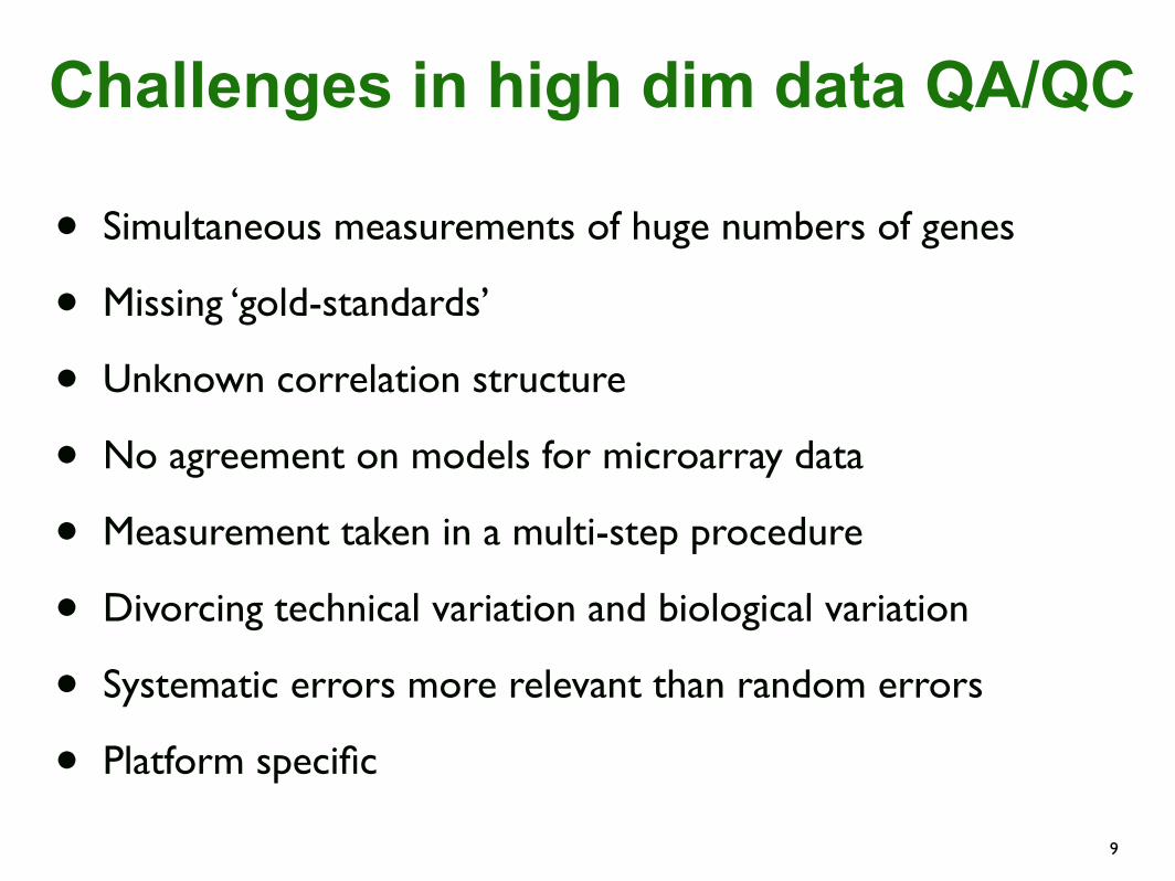
Challenges in high dim data QA/QC

• Simultaneous measurements of huge numbers of genes

• Missing ‘gold-standards’

• Unknown correlation structure

• No agreement on models for microarray data

• Measurement taken in a multi-step procedure

• Divorcing technical variation and biological variation

• Systematic errors more relevant than random errors

• Platform specific

9

Quality needsIndividual user (2-20 chips): Checking data quality for a

single experiment/study. Knowing what quality to expect at the design phase (e.g. for sample size).

Large multi-site study (100s of chips) : Comparing/combining data produced at different places, and different times.

Chip core facility (100s-1000s of chips): Developing/validating protocols. Monitoring routine performance.

Understanding quality: Impact of mRNA source (cell line, tissue, blood…), pooled mRNA or not, replicate type, replacement chips,…

Goals• Develop QA methods

• Link them to specific technical artifacts

• Study their properties

Joint work with Francois Collin, Ben Bolstad, Terry Speed (UC Berkeley)Technometrics, August 2008 (with discussion)

QA methods for short oligonucleotide microarray data

- Simultaneously for a batch of microarrays- After hybridization and data pre-processing

Approach

106

RMA Model

(”Robust Multi Array” (RMA) by Irizarry et al. 2002)

Fix gene (probe set). normalized background corrected PMs Probe effect and Array effect ,

and error (and sum zero constraint on probe effects)

Yjk = log2

Yjk = !j + "k + #jk

!k!j

107

Use IRWLS algorithm to fit RMA

rjk = Yjk ! estimator !j ! estimator "k

Iteratively minimize

S = MAD(rjk)

wjk = !(|rjk/S|)

robust estimator for scale

weights (of stand. resids.)

SE(final estimate !k) =1!Wk

Wk =!

j

wjkTotal probe weight

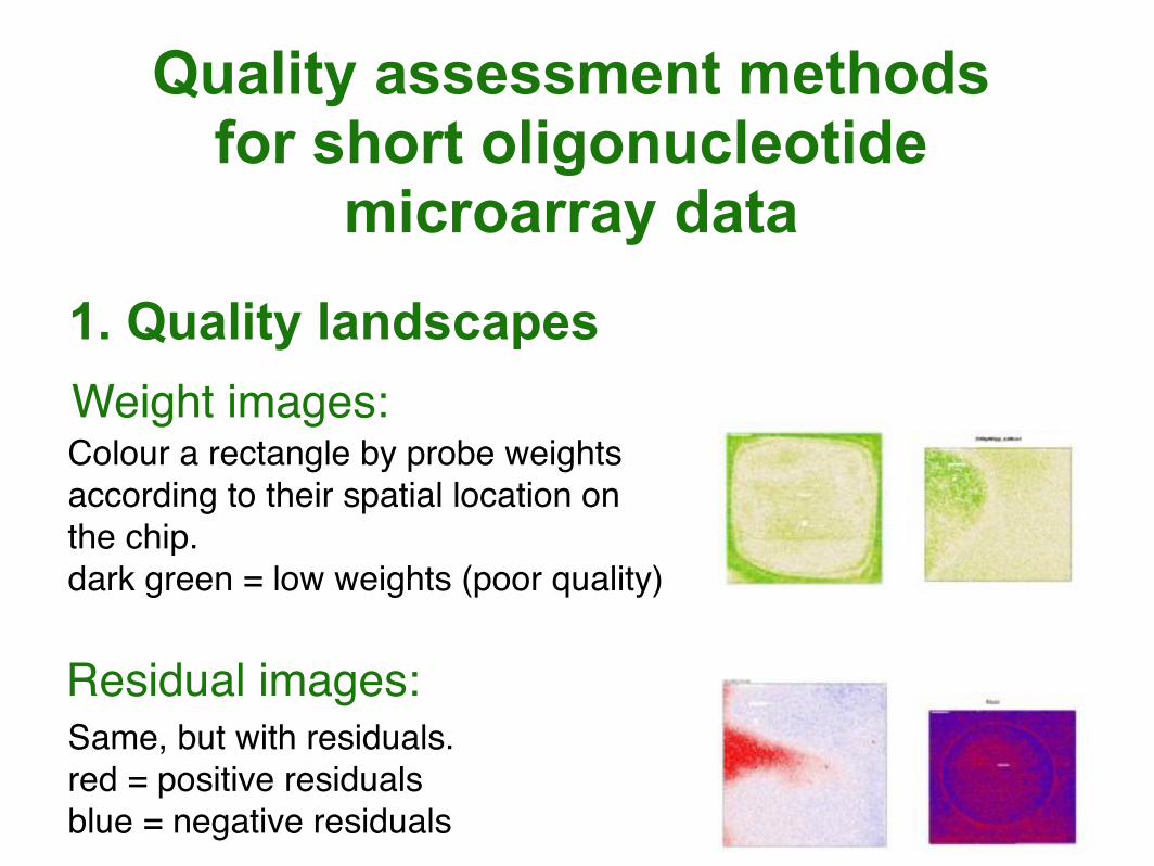
Weight images: 1. Quality landscapes

Colour a rectangle by probe weights according to their spatial location on the chip. dark green = low weights (poor quality)

Residual images: Same, but with residuals. red = positive residuals blue = negative residuals

Quality assessment methods for short oligonucleotide

microarray data

Fig. J1: “Bubbles” Fig. J2: “Circle and Stick” Fig. J3: “Sunset” Fig. J4: “Pond”

Fig. J5: “Letter S” Fig. J6: “Compartments” Fig. J7: “Triangle” Fig. J8: “Fingerprint”

Figures J1-8: Quality landscapes of some selected early St.Jude’s chips.

42www.stat.berkeley.edu/~bolstad/PLMImageGallery/index.html

3. Normalised unscaled standard error (NUSE):

NUSE :=Note:Normalisation because of heterogeneity in # effective probes

1!"

Wk

medk!1!"

Wk!

2. Relative Log Expression (RLE):

Median Chip: median expression over all arrays (gene by gene)RLE (gene A) in array k = log ratio gene Aʼs expression in array k and gene Aʼs median expression

Idea: use RLE distribution for quality assessment (QA).

Interpretation

Biologic assumptions

(A) majority of genes similar between different samples (B) # upregulated genes = # downregulated genes

Then, good quality is indicated by:

Med(NUSE)=1 small IQR(NUSE) Med(RLE)=0 small IQR(RLE)

Note: interpretation of the distributions rather than individual probe or probe set quantities

MLL - weightsNUSE

Weights

The MAS 5.0 quality report

• Background: No range. Key is consistency.

• Raw Q (Noise): Between 1.5 and 3.0 is ok.

• Percent present calls: Typical range is 20-50%.

• Scaling factor: Should be kept below 10. Key is consistency across arrays being analyzed.

• 3’/5’ ratios for GAPDH, BetaActin: less than 3.

• At 1.5 pM bioB should be called Present 70% of the time.

MLL 1

Median NUSE vs Affy quality report measures

Red pointer indicates the low quality chip.Affy quality report scores all in normal range.

medNUSE

%P

Noise

Scale factor

3’/5’

Is that really a bad array?

Confirmation: bias and spread in RLE

Case studies

17

Pritzker gender study data

• Tissue: Human brain regions dorso lateral prefrontal cortex (DLPFC) and cerebellum (CB)

• Hybridizations: 14 samples, hybridized in two labs (Irvine and Michigan), some data missing.

• Platform: Affymetrix HU95A.

Cerebellum

orange = Irvine, violet = Michigan

Lab difference in quality

Reason: insufficiently calibrated scanners.

Pritzker mood disorder data

• Tissue: Human brain regions from bipolar, major depression and control patients.

• Hybridizations: each hybridized in two lab out of 3s (Irvine, Davis and Michigan).

• Platform: Affymetrix HU133A,B.

• Done after gender study, after enormous effort to unify the conditions in the different labs.

Observation: Improved, but still noticable differences between labs.

Note: the boxplots are now of the the distribution of chip level quality scores (e.g. IQR(NUSE)) of all the chips in an experiment.

Drosophila mutant experiment (Tiago Magalhaes, Corey Lab, UC Berkeley)

• Tissue: 18 Drosophila mutants and 3 (kinds of) wild types

• Hybridizations: 3-5 per group, all by the same technician in UCB MCB (Cory lab)

Introducing the fruit fly: Drosophila Melanogaster

http://insects.eugenes.org/species/about/species-gallery/Drosophila_melanogaster/

For about 100 years Drosophila has been used as a model organism in genetic analyses. In fact much of our current knowledge on genes, development and genetic interactions originates from work with this system.One reason to choose Drosophila is its short life cycle.



Drosophila melanogaster Life Cycle

At room temperature – which for unknown reason corresponds to 25°C – generation time is about 10 days:

1 day embryogenesis1 day first instar larva1 day second instar larva2-3 days third instar larva5 days pupal stage

Drosophila mutant experiment

• Tiago Magalhaes, Corey Lab, UC Berkeley

• Tissue: 18 Drosophila mutants and 3 (kinds of) wild types

• Hybridizations: 3-5 per group, all by the same technician

• How do neurons find their correct targets, make appropriate synaptic connections, and set and adjust their size and strength?

• Find genes which regulate these mechanisms by comparing different mutants

• Loss Of Function (LOF) and Gain Of Functions (GOF) mutants for a number of proteins

Biological background about the study: Axon guidance in the Drosophila

central nervous system

• How do neurons find their correct targets, make appropriate synaptic connections, and set and adjust their size and strength?

• Find genes which regulate these mechanisms by comparing different mutants.

Biological questions:

Loss Of Function (LOF) and Gain Of Functions (GOF) mutants for a number of proteins:

• Robo: transmembrane protein, receptor for slit, negatively controlled by Comm

• Slit: extracellular protein, expressed by midline glia, ligand for Robo receptor

• Comm: surface protein, expressd on midline cells, transferred to commissural neurons

Phenotypes

AAAM

A

BBBM

B

CCCM

C

DDDM

D

EEEM

E

FFFM

F

GGGM

G

HHHM

H

IIIM

I

JJJM

J

KKKM

K

LLLM

L

MMMM

M

NNNM

N

OOOM

O

PPPM

P

QQQM

Q

RRRM

R

SSSM

S

TTTM

T

UUUM

U

VVVM

V

WWWM

W

XXXM

X

YYYM

Y

ZZZM

Z

aaaM

a

bbbM

b

cccM

c

dddM

d

eeeM

e

fffM

f

gggM

g

hhhM

h

iiiM

i

jjjM

j

kkkM

k

lllM

l

mmmM

m

nnnM

n

oooM

o

pppM

p

qqqM

q

rrrM

r

sssM

s

tttM

t

uuuM

u

vvvM

v

wwwM

w

xxxM

x

yyyM

y

zzzM

z

000M

0

111M

1

222M

2

333M

3

444M

4

555M

5

666M

6

777M

7

888M

8

999M

9

<<<M

<

===M

=

>>>M

>

???M

?

@@@M

@

###M

#

$$$M

$

&&&M

&

(((M

(

)))M

)

m88M8M

899M9M

91010M10M

101111M11M

11med(PM)Mmed(PM)M

med(PM)

xMxMPM.medMPM.medM

PM.med

AAAM

A

BBBM

B

CCCM

C

DDDM

D

EEEM

E

FFFM

F

GGGM

G

HHHM

H

IIIM

I

JJJM

J

KKKM

K

LLLM

L

MMMM

M

NNNM

N

OOOM

O

PPPM

P

QQQM

Q

RRRM

R

SSSM

S

TTTM

T

UUUM

U

VVVM

V

WWWM

W

XXXM

X

YYYM

Y

ZZZM

Z

aaaM

a

bbbM

b

cccM

c

dddM

d

eeeM

e

fffM

f

gggM

g

hhhM

h

iiiM

i

jjjM

j

kkkM

k

lllM

l

mmmM

m

nnnM

n

oooM

o

pppM

p

qqqM

q

rrrM

r

sssM

s

tttM

t

uuuM

u

vvvM

v

wwwM

w

xxxM

x

yyyM

y

zzzM

z

000M

0

111M

1

222M

2

333M

3

444M

4

555M

5

666M

6

777M

7

888M

8

999M

9

<<<M

<

===M

=

>>>M

>

???M

?

@@@M

@

###M

#

$$$M

$

&&&M

&

(((M

(

)))M

)

m1.61.6M1.6M

1.6

1.81.8M1.8M

1.8

2.02.0M2.0M

2.0

2.22.2M2.2M

2.2

2.42.4M2.4M

2.4

IQR(PM)MIQR(PM)M

IQR(PM)

xMxMPM.IQRMPM.IQRM

PM.IQR

AAAM

A

BBBM

B

CCCM

C

DDDM

D

EEEM

E

FFFM

F

GGGM

G

HHHM

H

IIIM

I

JJJM

J

KKKM

K

LLLM

L

MMMM

M

NNNM

N

OOOM

O

PPPM

P

QQQM

Q

RRRM

R

SSSM

S

TTTM

T

UUUM

U

VVVM

V

WWWM

W

XXXM

X

YYYM

Y

ZZZM

Z

aaaM

a

bbbM

b

cccM

c

dddM

d

eeeM

e

fffM

f

gggM

g

hhhM

h

iiiM

i

jjjM

j

kkkM

k

lllM

l

mmmM

m

nnnM

n

oooM

o

pppM

p

qqqM

q

rrrM

r

sssM

s

tttM

t

uuuM

u

vvvM

v

wwwM

w

xxxM

x

yyyM

y

zzzM

z

000M

0

111M

1

222M

2

333M

3

444M

4

555M

5

666M

6

777M

7

888M

8

999M

9

<<<M

<

===M

=

>>>M

>

???M

?

@@@M

@

###M

#

$$$M

$

&&&M

&

(((M

(

)))M

)

m0.000.00M0.00M

0.00

0.020.02M0.02M

0.02

0.040.04M0.04M

0.04

0.060.06M0.06M

0.06

0.080.08M0.08M

0.08

|med(RLE)|M|med(RLE)|M

|med(RLE)|

xMxMRLE.medMRLE.medM

RLE.med

AAAM

A

BBBM

B

CCCM

C

DDDM

D

EEEM

E

FFFM

F

GGGM

G

HHHM

H

IIIM

I

JJJM

J

KKKM

K

LLLM

L

MMMM

M

NNNM

N

OOOM

O

PPPM

P

QQQM

Q

RRRM

R

SSSM

S

TTTM

T

UUUM

U

VVVM

V

WWWM

W

XXXM

X

YYYM

Y

ZZZM

Z

aaaM

a

bbbM

b

cccM

c

dddM

d

eeeM

e

fffM

f

gggM

g

hhhM

h

iiiM

i

jjjM

j

kkkM

k

lllM

l

mmmM

m

nnnM

n

oooM

o

pppM

p

qqqM

q

rrrM

r

sssM

s

tttM

t

uuuM

u

vvvM

v

wwwM

w

xxxM

x

yyyM

y

zzzM

z

000M

0

111M

1

222M

2

333M

3

444M

4

555M

5

666M

6

777M

7

888M

8

999M

9

<<<M

<

===M

=

>>>M

>

???M

?

@@@M

@

###M

#

$$$M

$

&&&M

&

(((M

(

)))M

)

m0.150.15M0.15M

0.15

0.200.20M0.20M

0.20

0.250.25M0.25M

0.25

0.300.30M0.30M

0.30

0.350.35M0.35M

0.35

0.400.40M0.40M

0.40

0.450.45M0.45M

0.45

IQR(RLE)MIQR(RLE)M

IQR(RLE)

xMxMRLE.IQRMRLE.IQRM

RLE.IQR

AAAM

A

BBBM

B

CCCM

C

DDDM

D

EEEM

E

FFFM

F

GGGM

G

HHHM

H

IIIM

I

JJJM

J

KKKM

K

LLLM

L

MMMM

M

NNNM

N

OOOM

O

PPPM

P

QQQM

Q

RRRM

R

SSSM

S

TTTM

T

UUUM

U

VVVM

V

WWWM

W

XXXM

X

YYYM

Y

ZZZM

Z

aaaM

a

bbbM

b

cccM

c

dddM

d

eeeM

e

fffM

f

gggM

g

hhhM

h

iiiM

i

jjjM

j

kkkM

k

lllM

l

mmmM

m

nnnM

n

oooM

o

pppM

p

qqqM

q

rrrM

r

sssM

s

tttM

t

uuuM

u

vvvM

v

wwwM

w

xxxM

x

yyyM

y

zzzM

z

000M

0

111M

1

222M

2

333M

3

444M

4

555M

5

666M

6

777M

7

888M

8

999M

9

<<<M

<

===M

=

>>>M

>

???M

?

@@@M

@

###M

#

$$$M

$

&&&M

&

(((M

(

)))M

)

m0.980.98M0.98M

0.98

0.990.99M0.99M

0.99

1.001.00M1.00M

1.00

1.011.01M1.01M

1.01

1.021.02M1.02M

1.02

1.031.03M1.03M

1.03

1.041.04M1.04M

1.04

1.051.05M1.05M

1.05

med(Nuse)Mmed(Nuse)M

med(Nuse)

xMxMNuse.medMNuse.medM

Nuse.med

AAAM

A

BBBM

B

CCCM

C

DDDM

D

EEEM

E

FFFM

F

GGGM

G

HHHM

H

IIIM

I

JJJM

J

KKKM

K

LLLM

L

MMMM

M

NNNM

N

OOOM

O

PPPM

P

QQQM

Q

RRRM

R

SSSM

S

TTTM

T

UUUM

U

VVVM

V

WWWM

W

XXXM

X

YYYM

Y

ZZZM

Z

aaaM

a

bbbM

b

cccM

c

dddM

d

eeeM

e

fffM

f

gggM

g

hhhM

h

iiiM

i

jjjM

j

kkkM

k

lllM

l

mmmM

m

nnnM

n

oooM

o

pppM

p

qqqM

q

rrrM

r

sssM

s

tttM

t

uuuM

u

vvvM

v

wwwM

w

xxxM

x

yyyM

y

zzzM

z

000M

0

111M

1

222M

2

333M

3

444M

4

555M

5

666M

6

777M

7

888M

8

999M

9

<<<M

<

===M

=

>>>M

>

???M

?

@@@M

@

###M

#

$$$M

$

&&&M

&

(((M

(

)))M

)

m0.0200.020M0.020M

0.020

0.0250.025M0.025M

0.025

0.0300.030M0.030M

0.030

0.0350.035M0.035M

0.035

0.0400.040M0.040M

0.040

0.0450.045M0.045M

0.045

0.0500.050M0.050M

0.050

0.0550.055M0.055M

0.055

IQR(Nuse)MIQR(Nuse)M

IQR(Nuse)

xMxMNuse.IQRMNuse.IQRM

Nuse.IQR

QA on raw data may be misleading... Wild types Mutants

Quality measures: Affymetrix vs RMA based

Take home messages

132

Roles of statistics in genomics

Data preprocessing Linear models, robust stats, image analysis, industrial stats

Detection of d.e. genes Testing, multiple testing, resampling methods

Co-regulation Clustering, classification, Bayesian networks

Data QA/QC EDA, various stat. models

Experiment planning Experimental design, cost-benefit

Molecular diagnosisDecisions under uncertainty, risk interpretation/communication

Some of the tasks Some of the methods

David Hilbert:

The instrument that mediates between theory and practice, between thought and observation, is mathematics; it builds the bridge and makes it stronger and stronger.

Physics a century ago - biology today

Statistical mechanics Statistical genomics

Probabilistic models for description of a particle system on the microscopic level (including interactions)

Models for quantitative description of the interactions between molecules (genes & their products)

Thermodynamic limit: fluctuations become negligible, obtain macroscopic parameters

Some kind of data aggregation: explains phenotype of a cell, e.g. type, stage etc.

EARLY

STAGE

Differences: measurement technology, computational abilities...Similarities: formalization