mathematical preliminaries - introductory course on...
TRANSCRIPT
Vectors, tensors, and index notation Integral theorems Time-harmonic approach
Mathematical PreliminariesIntroductory Course on Multiphysics Modelling
TOMASZ G. ZIELINSKI
bluebox.ippt.pan.pl/˜tzielins/
Institute of Fundamental Technological Researchof the Polish Academy of Sciences
Warsaw • Poland
Vectors, tensors, and index notation Integral theorems Time-harmonic approach
Outline
1 Vectors, tensors, and index notationGeneralization of the concept of vectorSummation convention and index notationKronecker delta and permutation symbolTensors and their representationsMultiplication of vectors and tensorsVertical-bar convention and Nabla operator
2 Integral theoremsGeneral ideaStokes’ theoremGauss-Ostrogradsky theorem
3 Time-harmonic approachTypes of dynamic problemsComplex-valued notationA practical example

Vectors, tensors, and index notation Integral theorems Time-harmonic approach
Vectors, tensors, and index notationGeneralization of the concept of vector
A vector is a quantity that possesses both a magnitude and adirection and obeys certain laws (of vector algebra):• the vector addition and the commutative and associative laws,• the associative and distributive laws for the multiplication with
scalars.The vectors are suited to describe physical phenomena, sincethey are independent of any system of reference.
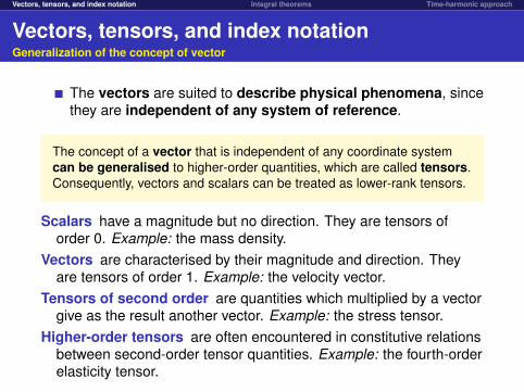
The concept of a vector that is independent of any coordinate systemcan be generalised to higher-order quantities, which are called tensors.Consequently, vectors and scalars can be treated as lower-rank tensors.
Scalars have a magnitude but no direction. They are tensors oforder 0. Example: the mass density.
Vectors are characterised by their magnitude and direction. Theyare tensors of order 1. Example: the velocity vector.
Tensors of second order are quantities which multiplied by a vectorgive as the result another vector. Example: the stress tensor.
Higher-order tensors are often encountered in constitutive relationsbetween second-order tensor quantities. Example: the fourth-orderelasticity tensor.
Vectors, tensors, and index notation Integral theorems Time-harmonic approach
Vectors, tensors, and index notationGeneralization of the concept of vector
The vectors are suited to describe physical phenomena, sincethey are independent of any system of reference.
The concept of a vector that is independent of any coordinate systemcan be generalised to higher-order quantities, which are called tensors.Consequently, vectors and scalars can be treated as lower-rank tensors.
Scalars have a magnitude but no direction. They are tensors oforder 0. Example: the mass density.
Vectors are characterised by their magnitude and direction. Theyare tensors of order 1. Example: the velocity vector.
Tensors of second order are quantities which multiplied by a vectorgive as the result another vector. Example: the stress tensor.
Higher-order tensors are often encountered in constitutive relationsbetween second-order tensor quantities. Example: the fourth-orderelasticity tensor.
Vectors, tensors, and index notation Integral theorems Time-harmonic approach
Vectors, tensors, and index notationSummation convention and index notation
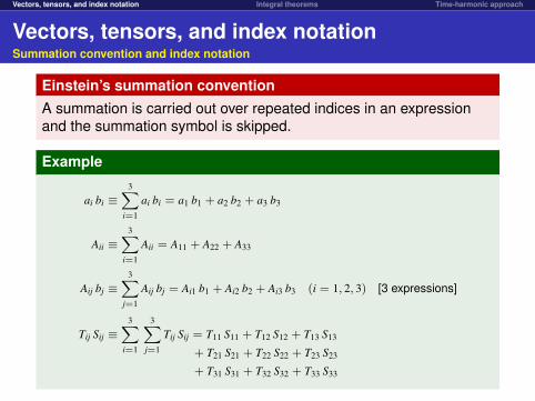
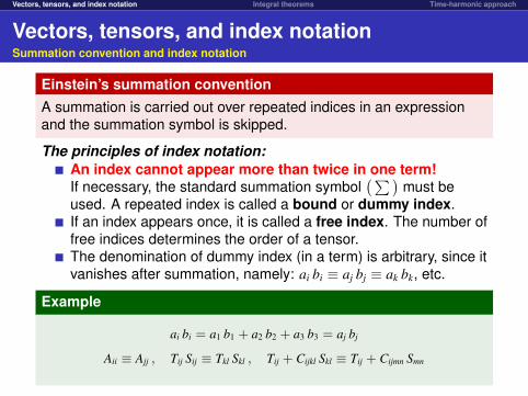
Einstein’s summation conventionA summation is carried out over repeated indices in an expressionand the summation symbol is skipped.
Example
ai bi ≡3∑
i=1
ai bi = a1 b1 + a2 b2 + a3 b3
Aii ≡3∑
i=1
Aii = A11 + A22 + A33
Aij bj ≡3∑
j=1
Aij bj = Ai1 b1 + Ai2 b2 + Ai3 b3 (i = 1, 2, 3) [3 expressions]
Tij Sij ≡3∑
i=1
3∑j=1
Tij Sij = T11 S11 + T12 S12 + T13 S13
+ T21 S21 + T22 S22 + T23 S23
+ T31 S31 + T32 S32 + T33 S33
The principles of index notation:An index cannot appear more than twice in one term!If necessary, the standard summation symbol
(∑)must be
used. A repeated index is called a bound or dummy index.
If an index appears once, it is called a free index. The number offree indices determines the order of a tensor.The denomination of dummy index (in a term) is arbitrary, since itvanishes after summation, namely: ai bi ≡ aj bj ≡ ak bk, etc.
Vectors, tensors, and index notation Integral theorems Time-harmonic approach
Vectors, tensors, and index notationSummation convention and index notation
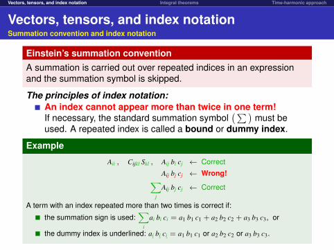
Einstein’s summation conventionA summation is carried out over repeated indices in an expressionand the summation symbol is skipped.
The principles of index notation:An index cannot appear more than twice in one term!If necessary, the standard summation symbol
(∑)must be
used. A repeated index is called a bound or dummy index.
Example
Aii , Cijkl Skl , Aij bi cj ← Correct
Aij bj cj ← Wrong!∑j
Aij bj cj ← Correct
A term with an index repeated more than two times is correct if:
the summation sign is used:∑
i
ai bi ci = a1 b1 c1 + a2 b2 c2 + a3 b3 c3, or
the dummy index is underlined: ai bi ci = a1 b1 c1 or a2 b2 c2 or a3 b3 c3.
If an index appears once, it is called a free index. The number offree indices determines the order of a tensor.The denomination of dummy index (in a term) is arbitrary, since itvanishes after summation, namely: ai bi ≡ aj bj ≡ ak bk, etc.

Vectors, tensors, and index notation Integral theorems Time-harmonic approach
Vectors, tensors, and index notationSummation convention and index notation
Einstein’s summation conventionA summation is carried out over repeated indices in an expressionand the summation symbol is skipped.
The principles of index notation:An index cannot appear more than twice in one term!If necessary, the standard summation symbol
(∑)must be
used. A repeated index is called a bound or dummy index.If an index appears once, it is called a free index. The number offree indices determines the order of a tensor.
Example
Aii , ai bi , Tij Sij ← scalars (no free indices)
Aij bj ← a vector (one free index: i)
Cijkl Skl ← a second-order tensor (two free indices: i, j)
The denomination of dummy index (in a term) is arbitrary, since itvanishes after summation, namely: ai bi ≡ aj bj ≡ ak bk, etc.
Vectors, tensors, and index notation Integral theorems Time-harmonic approach
Vectors, tensors, and index notationSummation convention and index notation
Einstein’s summation conventionA summation is carried out over repeated indices in an expressionand the summation symbol is skipped.
The principles of index notation:An index cannot appear more than twice in one term!If necessary, the standard summation symbol
(∑)must be
used. A repeated index is called a bound or dummy index.If an index appears once, it is called a free index. The number offree indices determines the order of a tensor.The denomination of dummy index (in a term) is arbitrary, since itvanishes after summation, namely: ai bi ≡ aj bj ≡ ak bk, etc.
Example
ai bi = a1 b1 + a2 b2 + a3 b3 = aj bj
Aii ≡ Ajj , Tij Sij ≡ Tkl Skl , Tij + Cijkl Skl ≡ Tij + Cijmn Smn

Vectors, tensors, and index notation Integral theorems Time-harmonic approach
Vectors, tensors, and index notationKronecker delta and permutation symbol
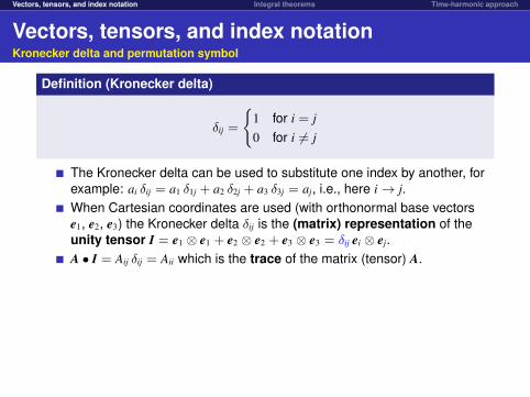
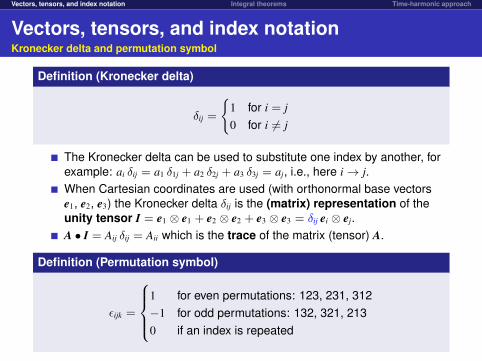
Definition (Kronecker delta)
δij =
{1 for i = j0 for i 6= j
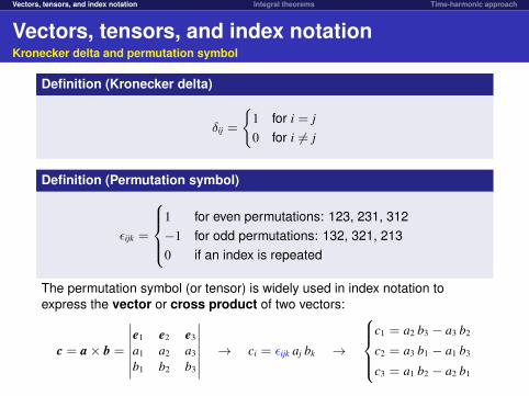
Definition (Permutation symbol)
εijk =
1 for even permutations: 123, 231, 312−1 for odd permutations: 132, 321, 2130 if an index is repeated
The permutation symbol (or tensor) is widely used in index notation toexpress the vector or cross product of two vectors:
c = a× b =
∣∣∣∣∣∣∣e1 e2 e3
a1 a2 a3
b1 b2 b3
∣∣∣∣∣∣∣ → ci = εijk aj bk →
c1 = a2 b3 − a3 b2
c2 = a3 b1 − a1 b3
c3 = a1 b2 − a2 b1
Vectors, tensors, and index notation Integral theorems Time-harmonic approach
Vectors, tensors, and index notationKronecker delta and permutation symbol
Definition (Kronecker delta)
δij =
{1 for i = j0 for i 6= j
The Kronecker delta can be used to substitute one index by another, forexample: ai δij = a1 δ1j + a2 δ2j + a3 δ3j = aj, i.e., here i→ j.When Cartesian coordinates are used (with orthonormal base vectorse1, e2, e3) the Kronecker delta δij is the (matrix) representation of theunity tensor I = e1 ⊗ e1 + e2 ⊗ e2 + e3 ⊗ e3 = δij ei ⊗ ej.A • I = Aij δij = Aii which is the trace of the matrix (tensor) A.
Definition (Permutation symbol)
εijk =
1 for even permutations: 123, 231, 312−1 for odd permutations: 132, 321, 2130 if an index is repeated
The permutation symbol (or tensor) is widely used in index notation toexpress the vector or cross product of two vectors:
c = a× b =
∣∣∣∣∣∣∣e1 e2 e3
a1 a2 a3
b1 b2 b3
∣∣∣∣∣∣∣ → ci = εijk aj bk →
c1 = a2 b3 − a3 b2
c2 = a3 b1 − a1 b3
c3 = a1 b2 − a2 b1
Vectors, tensors, and index notation Integral theorems Time-harmonic approach
Vectors, tensors, and index notationKronecker delta and permutation symbol
Definition (Kronecker delta)
δij =
{1 for i = j0 for i 6= j
Definition (Permutation symbol)
εijk =
1 for even permutations: 123, 231, 312−1 for odd permutations: 132, 321, 2130 if an index is repeated
The permutation symbol (or tensor) is widely used in index notation toexpress the vector or cross product of two vectors:
c = a× b =
∣∣∣∣∣∣∣e1 e2 e3
a1 a2 a3
b1 b2 b3
∣∣∣∣∣∣∣ → ci = εijk aj bk →
c1 = a2 b3 − a3 b2
c2 = a3 b1 − a1 b3
c3 = a1 b2 − a2 b1
Vectors, tensors, and index notation Integral theorems Time-harmonic approach
Vectors, tensors, and index notationTensors and their representations
Informal definition of tensorA tensor is a generalized linear ‘quantity’ that can be expressed asa multi-dimensional array relative to a choice of basis of theparticular space on which it is defined. Therefore:
a tensor is independent of any chosen frame of reference,its representation behaves in a specific way undercoordinate transformations.
Cartesian system of reference
Let E3 be the three-dimensional Euclidean space with a Cartesiancoordinate system with three orthonormal base vectors e1, e2, e3,so that
ei · ej = δij (i, j = 1, 2, 3).

Vectors, tensors, and index notation Integral theorems Time-harmonic approach
Vectors, tensors, and index notationTensors and their representations
Cartesian system of reference
Let E3 be the three-dimensional Euclidean space with a Cartesiancoordinate system with three orthonormal base vectors e1, e2, e3,so that
ei · ej = δij (i, j = 1, 2, 3).
A second-order tensor T ∈ E3 ⊗ E3 is defined by
T := Tij ei ⊗ ej = T11 e1 ⊗ e1 + T12 e1 ⊗ e2 + T13 e1 ⊗ e3
+ T21 e2 ⊗ e1 + T22 e2 ⊗ e2 + T23 e2 ⊗ e3
+ T31 e3 ⊗ e1 + T32 e3 ⊗ e2 + T33 e3 ⊗ e3
where ⊗ denotes the tensorial (or dyadic) product, and Tij is the(matrix) representation of T in the given frame of referencedefined by the base vectors e1, e2, e3.
Vectors, tensors, and index notation Integral theorems Time-harmonic approach
Vectors, tensors, and index notationTensors and their representations
A second-order tensor T ∈ E3 ⊗ E3 is defined by
T := Tij ei ⊗ ej = T11 e1 ⊗ e1 + T12 e1 ⊗ e2 + T13 e1 ⊗ e3
+ T21 e2 ⊗ e1 + T22 e2 ⊗ e2 + T23 e2 ⊗ e3
+ T31 e3 ⊗ e1 + T32 e3 ⊗ e2 + T33 e3 ⊗ e3
where ⊗ denotes the tensorial (or dyadic) product, and Tij is the(matrix) representation of T in the given frame of referencedefined by the base vectors e1, e2, e3.The second-order tensor T ∈ E3 ⊗ E3 can be viewed as a lineartransformation from E3 onto E3, meaning that it transformsevery vector v ∈ E3 into another vector from E3 as follows
T · v = (Tij ei ⊗ ej) · (vk ek) = Tij vk (
δjk︷ ︸︸ ︷ej · ek) ei
= Tij vk δjk ei = Tij vj ei = wi ei = w ∈ E3 where wi = Tij vj
Vectors, tensors, and index notation Integral theorems Time-harmonic approach
Vectors, tensors, and index notationTensors and their representations
A tensor of order n is defined by
nT := Tijk . . .︸ ︷︷ ︸
n indices
ei ⊗ ej ⊗ ek ⊗ . . .︸ ︷︷ ︸n terms
,
where Tijk... is its (n-dimensional array) representation in thegiven frame of reference.
Example
Let C ∈ E3 ⊗ E3 ⊗ E3 ⊗ E3 and S ∈ E3 ⊗ E3. The fourth-order tensor Cdescribes a linear transformation in E3 ⊗ E3:
C • S = C : S = (Cijkl ei ⊗ ej ⊗ ek ⊗ el) : (Smn em ⊗ en)
= Cijkl Smn (ek · em) (el · en) ei ⊗ ej
= Cijkl Smn δkm δln ei ⊗ ej = Cijkl Skl ei ⊗ ej
= Tij ei ⊗ ej = T ∈ E3 ⊗ E3 where Tij = Cijkl Skl
Vectors, tensors, and index notation Integral theorems Time-harmonic approach
Vectors, tensors, and index notationMultiplication of vectors and tensors
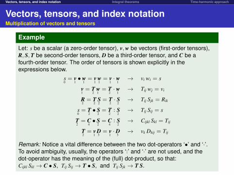
Example
Let: s be a scalar (a zero-order tensor), v,w be vectors (first-order tensors),R, S,T be second-order tensors, D be a third-order tensor, and C be afourth-order tensor. The order of tensors is shown explicitly in theexpressions below.
0s =
1v •
1w =
1v
1w =
1v ·
1w → vi wi = s
1v =
2T
1w =
2T ·
1w → Tij wj = vi
2R =
2T
2S =
2T ·
2S → Tij Sjk = Rik
0s =
2T •
2S =
2T :
2S → Tij Sij = s
2T =
4C •
2S =
4C :
2S → Cijkl Skl = Tij
2T =
1v
3D =
1v ·
3D → vk Dkij = Tij
Remark: Notice a vital difference between the two dot-operators ‘•’ and ‘·’.To avoid ambiguity, usually, the operators ‘:’ and ‘·’ are not used, and thedot-operator has the meaning of the (full) dot-product, so that:Cijkl Skl → C • S, Tij Sij → T • S, and Tij Sjk → T S.
Vectors, tensors, and index notation Integral theorems Time-harmonic approach
Vectors, tensors, and index notationVertical-bar convention and Nabla operator
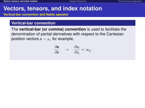
Vertical-bar conventionThe vertical-bar (or comma) convention is used to facilitate thedenomination of partial derivatives with respect to the Cartesianposition vectors x ∼ xi, for example,
∂u∂x
→ ∂ui
∂xj=: ui|j
�� ��∇× (∇s) = 0 (curl grad = 0)�� ��∇ · (∇× v) = 0 (div curl = 0)�� ��∇ · (∇s) = ∇2s (div grad = lapl)�� ��∇× (∇× v) = ∇(∇ · v)−∇2v (curl curl = grad div− lapl)
Vectors, tensors, and index notation Integral theorems Time-harmonic approach
Vectors, tensors, and index notationVertical-bar convention and Nabla operator
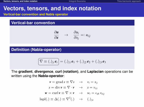
Vertical-bar convention
∂u∂x
→ ∂ui
∂xj=: ui|j
Definition (Nabla-operator)�� ��∇ ≡ (.)|i ei = (.)|1 e1 + (.)|2 e2 + (.)|3 e3
The gradient, divergence, curl (rotation), and Laplacian operations can bewritten using the Nabla-operator:
v = grad s ≡ ∇s → vi = s|is = div v ≡ ∇ · v → s = vi|i
w = curl v ≡ ∇× v → wi = εijk vk|j
lapl(.) ≡ ∆(.) ≡ ∇2(.) → (.)|ii
�� ��∇× (∇s) = 0 (curl grad = 0)�� ��∇ · (∇× v) = 0 (div curl = 0)�� ��∇ · (∇s) = ∇2s (div grad = lapl)�� ��∇× (∇× v) = ∇(∇ · v)−∇2v (curl curl = grad div− lapl)

Vectors, tensors, and index notation Integral theorems Time-harmonic approach
Vectors, tensors, and index notationNabla-operator and vector calculus identities�� ��∇ ≡ (.)|i ei = (.)|1 e1 + (.)|2 e2 + (.)|3 e3
v = grad s ≡ ∇s → vi = s|iT = grad v ≡ ∇⊗ v → Tij = vi|j
s = div v ≡ ∇ · v → s = vi|i
v = div T ≡ ∇ · T → vi = Tji|j
w = curl v ≡ ∇× v → wi = εijk vk|j
lapl(.) ≡ ∆(.) ≡ ∇2(.) → (.)|ii
Some vector calculus identities:�� ��∇× (∇s) = 0 (curl grad = 0)�� ��∇ · (∇× v) = 0 (div curl = 0)�� ��∇ · (∇s) = ∇2s (div grad = lapl)�� ��∇× (∇× v) = ∇(∇ · v)−∇2v (curl curl = grad div− lapl)
Vectors, tensors, and index notation Integral theorems Time-harmonic approach
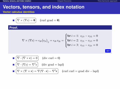
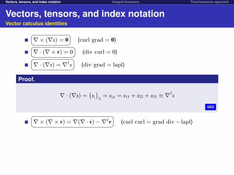
Vectors, tensors, and index notationVector calculus identities�� ��∇× (∇s) = 0 (curl grad = 0)
Proof.
∇× (∇s) = εijk(s|k)|j = εijk s|kj =
for i = 1: s|23 − s|32 = 0
for i = 2: s|31 − s|13 = 0
for i = 3: s|12 − s|21 = 0
QED�� ��∇ · (∇× v) = 0 (div curl = 0)�� ��∇ · (∇s) = ∇2s (div grad = lapl)�� ��∇× (∇× v) = ∇(∇ · v)−∇2v (curl curl = grad div− lapl)

Vectors, tensors, and index notation Integral theorems Time-harmonic approach
Vectors, tensors, and index notationVector calculus identities�� ��∇× (∇s) = 0 (curl grad = 0)�� ��∇ · (∇× v) = 0 (div curl = 0)
Proof.
∇ · (∇× v) =(εijk vk|j
)|i = εijk vk|ji
=(v3|21 − v3|12
)+(v1|32 − v1|23
)+(v2|13 − v2|31
)= 0
QED�� ��∇ · (∇s) = ∇2s (div grad = lapl)�� ��∇× (∇× v) = ∇(∇ · v)−∇2v (curl curl = grad div− lapl)
Vectors, tensors, and index notation Integral theorems Time-harmonic approach
Vectors, tensors, and index notationVector calculus identities�� ��∇× (∇s) = 0 (curl grad = 0)�� ��∇ · (∇× v) = 0 (div curl = 0)�� ��∇ · (∇s) = ∇2s (div grad = lapl)
Proof.
∇ · (∇s) =(s|)|i = s|ii = s11 + s22 + s33 ≡ ∇2s
QED�� ��∇× (∇× v) = ∇(∇ · v)−∇2v (curl curl = grad div− lapl)
Vectors, tensors, and index notation Integral theorems Time-harmonic approach
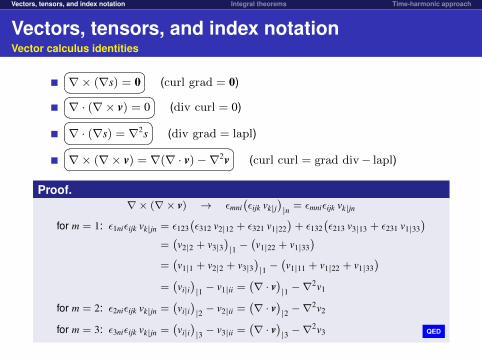
Vectors, tensors, and index notationVector calculus identities�� ��∇× (∇s) = 0 (curl grad = 0)�� ��∇ · (∇× v) = 0 (div curl = 0)�� ��∇ · (∇s) = ∇2s (div grad = lapl)�� ��∇× (∇× v) = ∇(∇ · v)−∇2v (curl curl = grad div− lapl)
Proof.∇× (∇× v) → εmni
(εijk vk|j
)|n = εmniεijk vk|jn
for m = 1: ε1niεijk vk|jn = ε123(ε312 v2|12 + ε321 v1|22
)+ ε132
(ε213 v3|13 + ε231 v1|33
)=(v2|2 + v3|3
)|1 −
(v1|22 + v1|33
)=(v1|1 + v2|2 + v3|3
)|1 −
(v1|11 + v1|22 + v1|33
)=(vi|i)|1 − v1|ii =
(∇ · v
)|1 −∇
2v1
for m = 2: ε2niεijk vk|jn =(vi|i)|2 − v2|ii =
(∇ · v
)|2 −∇
2v2
for m = 3: ε3niεijk vk|jn =(vi|i)|3 − v3|ii =
(∇ · v
)|3 −∇
2v3 QED

Vectors, tensors, and index notation Integral theorems Time-harmonic approach
Outline
1 Vectors, tensors, and index notationGeneralization of the concept of vectorSummation convention and index notationKronecker delta and permutation symbolTensors and their representationsMultiplication of vectors and tensorsVertical-bar convention and Nabla operator
2 Integral theoremsGeneral ideaStokes’ theoremGauss-Ostrogradsky theorem
3 Time-harmonic approachTypes of dynamic problemsComplex-valued notationA practical example
Vectors, tensors, and index notation Integral theorems Time-harmonic approach
Integral theoremsGeneral idea
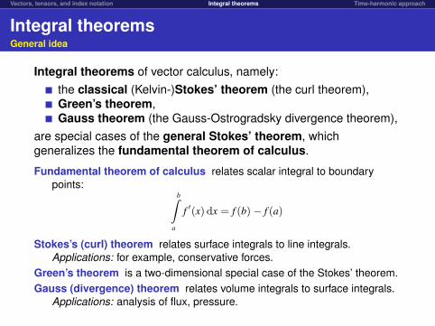
Integral theorems of vector calculus, namely:the classical (Kelvin-)Stokes’ theorem (the curl theorem),Green’s theorem,Gauss theorem (the Gauss-Ostrogradsky divergence theorem),
are special cases of the general Stokes’ theorem, whichgeneralizes the fundamental theorem of calculus.
Fundamental theorem of calculus relates scalar integral to boundarypoints:
b∫a
f ′(x) dx = f (b)− f (a)
Stokes’s (curl) theorem relates surface integrals to line integrals.Applications: for example, conservative forces.
Green’s theorem is a two-dimensional special case of the Stokes’ theorem.Gauss (divergence) theorem relates volume integrals to surface integrals.
Applications: analysis of flux, pressure.
Vectors, tensors, and index notation Integral theorems Time-harmonic approach
Integral theoremsGeneral idea
Integral theorems of vector calculus, namely:the classical (Kelvin-)Stokes’ theorem (the curl theorem),Green’s theorem,Gauss theorem (the Gauss-Ostrogradsky divergence theorem),
are special cases of the general Stokes’ theorem, whichgeneralizes the fundamental theorem of calculus.
Fundamental theorem of calculus relates scalar integral to boundarypoints:
b∫a
f ′(x) dx = f (b)− f (a)
Stokes’s (curl) theorem relates surface integrals to line integrals.Applications: for example, conservative forces.
Green’s theorem is a two-dimensional special case of the Stokes’ theorem.Gauss (divergence) theorem relates volume integrals to surface integrals.
Applications: analysis of flux, pressure.
Vectors, tensors, and index notation Integral theorems Time-harmonic approach
Integral theoremsStokes’ theorem
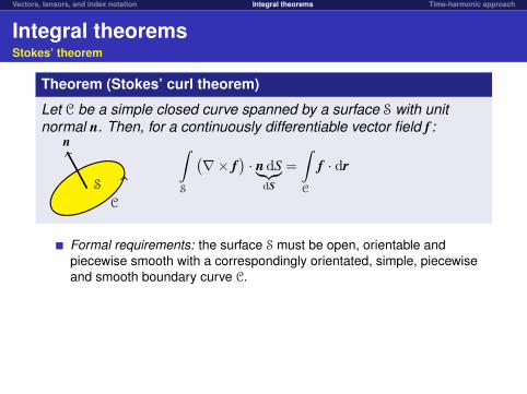
Theorem (Stokes’ curl theorem)
Let C be a simple closed curve spanned by a surface S with unitnormal n. Then, for a continuously differentiable vector field f :∫
S
(∇× f
)· n dS︸︷︷︸
dS
=
∫C
f · dr
n
S
C
Formal requirements: the surface S must be open, orientable andpiecewise smooth with a correspondingly orientated, simple, piecewiseand smooth boundary curve C.
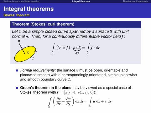
Green’s theorem in the plane may be viewed as a special case ofStokes’ theorem (with f =
[u(x, y), v(x, y), 0
]):∫
S
(∂v∂x− ∂u∂y
)dx dy =
∫C
u dx + v dy
Vectors, tensors, and index notation Integral theorems Time-harmonic approach
Integral theoremsStokes’ theorem
Theorem (Stokes’ curl theorem)
Let C be a simple closed curve spanned by a surface S with unitnormal n. Then, for a continuously differentiable vector field f :∫
S
(∇× f
)· n dS︸︷︷︸
dS
=
∫C
f · dr
n
S
C
Formal requirements: the surface S must be open, orientable andpiecewise smooth with a correspondingly orientated, simple, piecewiseand smooth boundary curve C.
Green’s theorem in the plane may be viewed as a special case ofStokes’ theorem (with f =
[u(x, y), v(x, y), 0
]):∫
S
(∂v∂x− ∂u∂y
)dx dy =
∫C
u dx + v dy
Vectors, tensors, and index notation Integral theorems Time-harmonic approach
Integral theoremsStokes’ theorem
Theorem (Stokes’ curl theorem)
Let C be a simple closed curve spanned by a surface S with unitnormal n. Then, for a continuously differentiable vector field f :∫
S
(∇× f
)· n dS︸︷︷︸
dS
=
∫C
f · dr
n
S
C
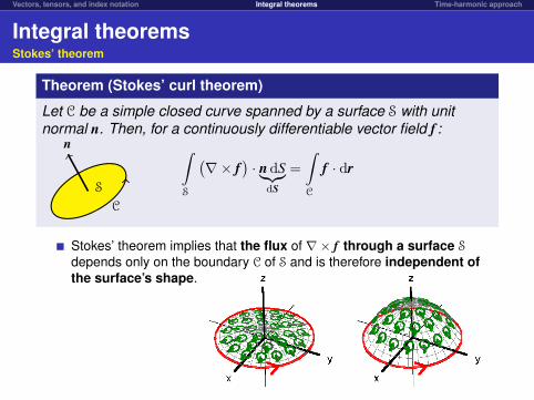
Stokes’ theorem implies that the flux of ∇× f through a surface S
depends only on the boundary C of S and is therefore independent ofthe surface’s shape.
Green’s theorem in the plane may be viewed as a special case ofStokes’ theorem (with f =
[u(x, y), v(x, y), 0
]):∫
S
(∂v∂x− ∂u∂y
)dx dy =
∫C
u dx + v dy
Vectors, tensors, and index notation Integral theorems Time-harmonic approach
Integral theoremsGauss-Ostrogradsky theorem
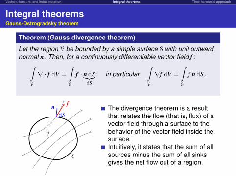
Theorem (Gauss divergence theorem)
Let the region V be bounded by a simple surface S with unit outwardnormal n. Then, for a continuously differentiable vector field f :∫
V
∇ · f dV =
∫S
f · n dS︸︷︷︸dS
; in particular∫V
∇f dV =
∫S
f n dS .
S
V
dSn f
The divergence theorem is a resultthat relates the flow (that is, flux) of avector field through a surface to thebehavior of the vector field inside thesurface.Intuitively, it states that the sum of allsources minus the sum of all sinksgives the net flow out of a region.
Vectors, tensors, and index notation Integral theorems Time-harmonic approach
Outline
1 Vectors, tensors, and index notationGeneralization of the concept of vectorSummation convention and index notationKronecker delta and permutation symbolTensors and their representationsMultiplication of vectors and tensorsVertical-bar convention and Nabla operator
2 Integral theoremsGeneral ideaStokes’ theoremGauss-Ostrogradsky theorem
3 Time-harmonic approachTypes of dynamic problemsComplex-valued notationA practical example
Vectors, tensors, and index notation Integral theorems Time-harmonic approach
Time-harmonic approachTypes of dynamic problems
Dynamic problems. In dynamic problems, the field variablesdepend upon position x and time t, for example, u = u(x, t).
Time-harmonic solution:
u(x, t) = u(x) cos(ω t + α(x)
)where: ω = 2π f is called the angular (or circular) frequency,α(x) is the phase-angle shift, and u(x) can be interpreted as aspatial amplitude.
A complex-valued notation for time-harmonic problems
A convenient way to handle time-harmonic problems is in the complexnotation with the real part as a physically meaningful solution:
u(x, t) = u(x) cos(ω t + α(x)
)= u Re
{ exp[(i(ω t+α)]︷ ︸︸ ︷cos(ω t + α) + i sin(ω t + α)
}= u Re
{exp[(i(ω t + α)]
}= Re
{u exp(iα)︸ ︷︷ ︸
u
exp(iω t)}
= Re{
u exp(iω t)}
where the so-called complex amplitude (or phasor) is introduced:
u = u(x) = u(x) exp(iα(x)
)= u(x)
(cosα(x) + i sinα(x)
)
Vectors, tensors, and index notation Integral theorems Time-harmonic approach
Time-harmonic approachTypes of dynamic problems
Dynamic problems. In dynamic problems, the field variablesdepend upon position x and time t, for example, u = u(x, t).
Separation of variables. In many cases, the governing PDEs can besolved by expressing u as a product of functions that each dependonly on one of the independent variables: u(x, t) = u(x) u(t).
Time-harmonic solution:
u(x, t) = u(x) cos(ω t + α(x)
)where: ω = 2π f is called the angular (or circular) frequency,α(x) is the phase-angle shift, and u(x) can be interpreted as aspatial amplitude.
A complex-valued notation for time-harmonic problems
A convenient way to handle time-harmonic problems is in the complexnotation with the real part as a physically meaningful solution:
u(x, t) = u(x) cos(ω t + α(x)
)= u Re
{ exp[(i(ω t+α)]︷ ︸︸ ︷cos(ω t + α) + i sin(ω t + α)
}= u Re
{exp[(i(ω t + α)]
}= Re
{u exp(iα)︸ ︷︷ ︸
u
exp(iω t)}
= Re{
u exp(iω t)}
where the so-called complex amplitude (or phasor) is introduced:
u = u(x) = u(x) exp(iα(x)
)= u(x)
(cosα(x) + i sinα(x)
)

Vectors, tensors, and index notation Integral theorems Time-harmonic approach
Time-harmonic approachTypes of dynamic problems
Dynamic problems. In dynamic problems, the field variablesdepend upon position x and time t, for example, u = u(x, t).
Separation of variables. In many cases, the governing PDEs can besolved by expressing u as a product of functions that each dependonly on one of the independent variables: u(x, t) = u(x) u(t).
Steady state. A system is in steady state if its recently observedbehaviour will continue into the future. An opposite situation iscalled the transient state which is often a start-up in manysteady state systems. An important case of steady state is thetime-harmonic behaviour.
Time-harmonic solution. If the time-dependent function u(t) is atime-harmonic function (with the frequency f ), the solution can bewritten as
u(x, t) = u(x) cos(ω t + α(x)
)where: ω = 2π f is called the angular (or circular) frequency,α(x) is the phase-angle shift, and u(x) can be interpreted as aspatial amplitude.
A complex-valued notation for time-harmonic problems
A convenient way to handle time-harmonic problems is in the complexnotation with the real part as a physically meaningful solution:
u(x, t) = u(x) cos(ω t + α(x)
)= u Re
{ exp[(i(ω t+α)]︷ ︸︸ ︷cos(ω t + α) + i sin(ω t + α)
}= u Re
{exp[(i(ω t + α)]
}= Re
{u exp(iα)︸ ︷︷ ︸
u
exp(iω t)}
= Re{
u exp(iω t)}
where the so-called complex amplitude (or phasor) is introduced:
u = u(x) = u(x) exp(iα(x)
)= u(x)
(cosα(x) + i sinα(x)
)
Vectors, tensors, and index notation Integral theorems Time-harmonic approach
Time-harmonic approachComplex-valued notation
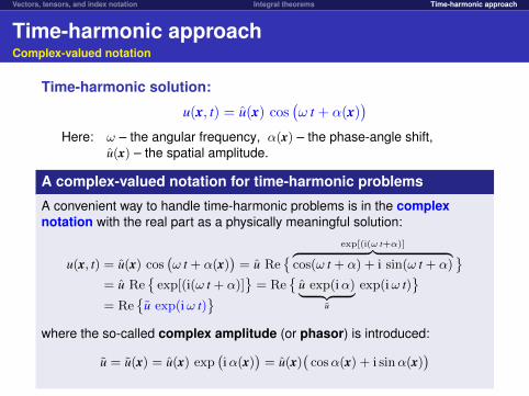
Time-harmonic solution:
u(x, t) = u(x) cos(ω t + α(x)
)Here: ω – the angular frequency, α(x) – the phase-angle shift,
u(x) – the spatial amplitude.
A complex-valued notation for time-harmonic problems
A convenient way to handle time-harmonic problems is in the complexnotation with the real part as a physically meaningful solution:
u(x, t) = u(x) cos(ω t + α(x)
)= u Re
{ exp[(i(ω t+α)]︷ ︸︸ ︷cos(ω t + α) + i sin(ω t + α)
}= u Re
{exp[(i(ω t + α)]
}= Re
{u exp(iα)︸ ︷︷ ︸
u
exp(iω t)}
= Re{
u exp(iω t)}
where the so-called complex amplitude (or phasor) is introduced:
u = u(x) = u(x) exp(iα(x)
)= u(x)
(cosα(x) + i sinα(x)
)

Vectors, tensors, and index notation Integral theorems Time-harmonic approach
Time-harmonic approachA practical example
Consider a linear dynamic system characterized by the matrices ofstiffness K, damping C, and mass M:
K q(t) + C q(t) + M q(t) = Q(t)
where Q(t) is the dynamic excitation (a time-varying force) and q(t) isthe system’s response (displacement).
Vectors, tensors, and index notation Integral theorems Time-harmonic approach
Time-harmonic approachA practical example
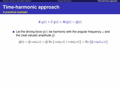
K q(t) + C q(t) + M q(t) = Q(t)
Let the driving force Q(t) be harmonic with the angular frequency ω andthe (real-valued) amplitude Q:
Q(t) = Q cos(ω t) = Q Re{
cos(ω t) + i sin(ω t)}
= Re{
Q exp(iω t)}

Vectors, tensors, and index notation Integral theorems Time-harmonic approach
Time-harmonic approachA practical example
K q(t) + C q(t) + M q(t) = Q(t)
Let the driving force Q(t) be harmonic with the angular frequency ω andthe (real-valued) amplitude Q:
Q(t) = Q cos(ω t) = Q Re{
cos(ω t) + i sin(ω t)}
= Re{
Q exp(iω t)}
Since the system is linear the response q(t) will be also harmonic andwith the same angular frequency but shifted by the phase angle α:
q(t) = q cos(ω t + α) = q Re{
cos(ω t + α) + i sin(ω t + α)}
= q Re{
exp[i(ω t + α)]}
= Re{
q exp(iα)︸ ︷︷ ︸q
exp(iω t)}
= Re{
q exp(iω t)}
Here, q and q are the real and complex amplitudes, respectively. Thereal amplitude q and the phase angle α are unknowns; thus, unknown isthe complex amplitude q = q
(cosα+ i sinα
).

Vectors, tensors, and index notation Integral theorems Time-harmonic approach
Time-harmonic approachA practical example
K q(t) + C q(t) + M q(t) = Q(t)
Now, one can substitute into the system’s equation
Q(t) ← Q exp(iω t) ,
q(t) ← q exp(iω t) , q(t) = q iω exp(iω t) , q(t) = −qω2 exp(iω t)
to obtain the following algebraic equation for the unknown complexamplitude q: [
K + iω C − ω2 M]q = Q
Vectors, tensors, and index notation Integral theorems Time-harmonic approach
Time-harmonic approachA practical example
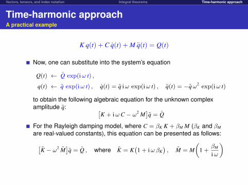
K q(t) + C q(t) + M q(t) = Q(t)
Now, one can substitute into the system’s equation
Q(t) ← Q exp(iω t) ,
q(t) ← q exp(iω t) , q(t) = q iω exp(iω t) , q(t) = −qω2 exp(iω t)
to obtain the following algebraic equation for the unknown complexamplitude q: [
K + iω C − ω2 M]q = Q
For the Rayleigh damping model, where C = βK K + βM M (βK and βM
are real-valued constants), this equation can be presented as follows:
[K − ω2 M
]q = Q , where K = K
(1 + iω βK
), M = M
(1 +
βM
iω
)
Vectors, tensors, and index notation Integral theorems Time-harmonic approach
Time-harmonic approachA practical example
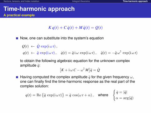
K q(t) + C q(t) + M q(t) = Q(t)
Now, one can substitute into the system’s equation
Q(t) ← Q exp(iω t) ,
q(t) ← q exp(iω t) , q(t) = q iω exp(iω t) , q(t) = −qω2 exp(iω t)
to obtain the following algebraic equation for the unknown complexamplitude q: [
K + iω C − ω2 M]q = Q
Having computed the complex amplitude q for the given frequency ω,one can finally find the time-harmonic response as the real part of thecomplex solution:
q(t) = Re{
q exp(iω t)}
= q cos(ω t + α) , where
{q = |q|α = arg(q)