matlab - fachbereich mathematik | universität stuttgart · matlab prof. dr. klaus h ollig institut...
TRANSCRIPT
Matlab
Prof. Dr. Klaus Hollig
Institut fur Mathematischen Methoden in den Ingenieurwissenschaften,Numerik und Geometrische Modellierung
Prof. Dr. Klaus Hollig (IMNG) Matlab 1 / 1
Grafik Darstellung von Funktionen und Kurven
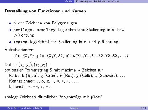
Darstellung von Funktionen und Kurven
plot: Zeichnen von Polygonzugen
semilogx, semilogy: logarithmische Skalierung in x- bzw.y -Richtung
loglog: logarithmische Skalierung in x- und y -Richtung
Aufrufvarianten:
plot(X,Y), plot(X,Y,S), plot(X1,Y1,S1,X2,Y2,S2,...)
Daten: (x1, y1), (x2, y2), . . .optionaler Formatstring S mit maximal 4 Zeichen fur
Farbe: b (Blau), g (Grun), r (Rot), y (Gelb), k (Schwarz), . . .Kennzeichner: ., o, x, +, *, <, >, . . .Linienstil: -, --, :, -.
analog: Zeichnen raumlicher Polygonzuge mit plot3
Prof. Dr. Klaus Hollig (IMNG) Matlab 2 / 1
Grafik Darstellung von Funktionen und Kurven
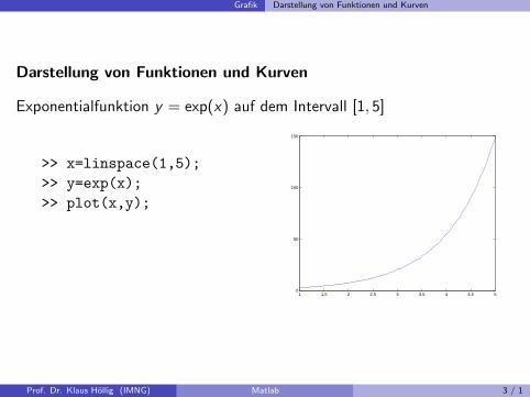
Darstellung von Funktionen und Kurven
Exponentialfunktion y = exp(x) auf dem Intervall [1, 5]
>> x=linspace(1,5);>> y=exp(x);>> plot(x,y);
1 1.5 2 2.5 3 3.5 4 4.5 50
50
100
150
Prof. Dr. Klaus Hollig (IMNG) Matlab 3 / 1
Grafik Darstellung von Funktionen und Kurven
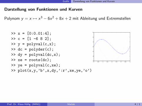
Darstellung von Funktionen und Kurven
Polynom y = x 7→ x3 − 6x2 + 8x + 2 mit Ableitung und Extremstellen
>> x = [0:0.01:4];>> c = [1 -6 8 2];>> y = polyval(c,x);>> dc = polyder(c);>> dy = polyval(dc,x);>> xe = roots(dc);>> ye = polyval(c,xe);>> plot(x,y,’b’,x,dy,’:r’,xe,ye,’o’)
0 0.5 1 1.5 2 2.5 3 3.5 4−4
−2
0
2
4
6
8
Prof. Dr. Klaus Hollig (IMNG) Matlab 4 / 1
Grafik Darstellung von Funktionen und Kurven
Darstellung von Funktionen und Kurven
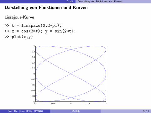
Lissajous-Kurve
>> t = linspace(0,2*pi);>> x = cos(3*t); y = sin(2*t);>> plot(x,y)
−1 −0.5 0 0.5 1−1
−0.8
−0.6
−0.4
−0.2
0
0.2
0.4
0.6
0.8
1
Prof. Dr. Klaus Hollig (IMNG) Matlab 5 / 1
Grafik Diagramme
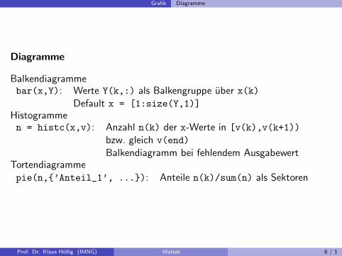
Diagramme
Balkendiagrammebar(x,Y): Werte Y(k,:) als Balkengruppe uber x(k)
Default x = [1:size(Y,1)]Histogrammen = histc(x,v): Anzahl n(k) der x-Werte in [v(k),v(k+1))
bzw. gleich v(end)Balkendiagramm bei fehlendem Ausgabewert
Tortendiagrammepie(n,{’Anteil_1’, ...}): Anteile n(k)/sum(n) als Sektoren
Prof. Dr. Klaus Hollig (IMNG) Matlab 6 / 1

Grafik Diagramme
Diagramme
>> % Tages- und Nachttemperaturen im monatlichen Mittel>> bar(degrees);>> average = sum(degrees’)/2;>> months = histc(average,[-inf 1 11 21 inf]);>> pie(months(1:end-1),{’<=0 Grad’, ’1...10 Grad’, ...
’11...20 Grad’, ’>20 Grad’})
1 2 3 4 5 6 7 8 9 10 11 12−15
−10
−5
0
5
10
15
20
25
30
35
<=0 Grad
1...10 Grad 11...20 Grad
>20 Grad
Prof. Dr. Klaus Hollig (IMNG) Matlab 7 / 1
Grafik Modifikation des Koordinatensystems und dessen Darstellung
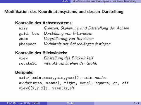
Modifikation des Koordinatensystems und dessen Darstellung
Kontrolle des Achsensystems:axis Grenzen, Skalierung und Darstellung der Achsengrid, box Darstellung von Gitterlinienzoom Vergroßerung von Bereichenpbaspect Verhaltnis der Achsenlangen festlegen
Kontrolle des Blickwinkels:view Einstellung des Blickwinkelsrotate3d interaktives Drehen der Grafik
Beispiele:axis([xmin,xmax,ymin,ymax]), axis modusmodus: auto, manual, tight, equal, square, on, offview([x,y,z]), view(az,el)
Prof. Dr. Klaus Hollig (IMNG) Matlab 8 / 1
Grafik Beschriftung von Grafiken
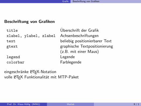
Beschriftung von Grafiken
title Uberschrift der Grafikxlabel, ylabel, zlabel Achsenbeschriftungentext beliebig positionierbarer Textgtext graphische Textpositionierung
(z.B. mit einer Maus)legend Legendecolorbar Farblegende
eingeschranke LATEX-Notationvolle LATEX Funktionalitat mit MTP-Paket
Prof. Dr. Klaus Hollig (IMNG) Matlab 9 / 1

Grafik Beschriftung von Grafiken
Beschriftung von Grafiken
>> x=linspace(0,2*pi);>> plot(x,[sin(x);cos(x)])>> title(’Trigonometrische Funktionen’)>> xlabel(’Winkel \alpha’)>> ylabel(’Funktionswerte’)>> text(pi/4,sin(pi/4),’ sin \pi/4=cos \pi/4’)>> legend({’sin \alpha’,’cos \alpha’},’Location’,’EastOutside’)>> axis equal>> axis tight
0 1 2 3 4 5 6
−0.5
0
0.5
1Trigonometrische Funktionen
Winkel α
Fun
ktio
nsw
erte
sin π/4=cos π/4
sin αcos α
Prof. Dr. Klaus Hollig (IMNG) Matlab 10 / 1
Grafik Darstellung bivariater Funktionen und Flachen
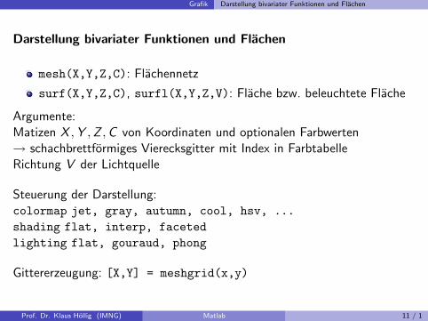
Darstellung bivariater Funktionen und Flachen
mesh(X,Y,Z,C): Flachennetz
surf(X,Y,Z,C), surfl(X,Y,Z,V): Flache bzw. beleuchtete Flache
Argumente:Matizen X , Y , Z , C von Koordinaten und optionalen Farbwerten→ schachbrettformiges Vierecksgitter mit Index in FarbtabelleRichtung V der Lichtquelle
Steuerung der Darstellung:colormap jet, gray, autumn, cool, hsv, ...shading flat, interp, facetedlighting flat, gouraud, phong
Gittererzeugung: [X,Y] = meshgrid(x,y)
Prof. Dr. Klaus Hollig (IMNG) Matlab 11 / 1
Grafik Darstellung bivariater Funktionen und Flachen
Darstellung bivariater Funktionen und Flachen
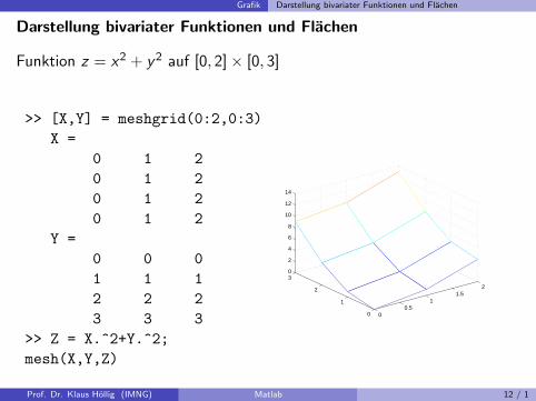
Funktion z = x2 + y 2 auf [0, 2]× [0, 3]
>> [X,Y] = meshgrid(0:2,0:3)X =
0 1 20 1 20 1 20 1 2
Y =0 0 01 1 12 2 23 3 3
>> Z = X.^2+Y.^2;mesh(X,Y,Z)
00.5
11.5
2
0
1
2
30
2
4
6
8
10
12
14
Prof. Dr. Klaus Hollig (IMNG) Matlab 12 / 1

Grafik Darstellung bivariater Funktionen und Flachen
Darstellung bivariater Funktionen und Flachen
Einheitsphare, parametrisiert mit Hilfe von Kugelkoordinaten
>> [p,t]=meshgrid(...linspace(-pi,pi,30),...linspace(0,pi,15));
>> X=cos(p).*sin(t);>> Y=sin(p).*sin(t);>> Z=cos(t);>> surf(X,Y,Z); −1
−0.5
0
0.5
1
−1
−0.5
0
0.5
1−1
−0.5
0
0.5
1
Prof. Dr. Klaus Hollig (IMNG) Matlab 13 / 1
Grafik Darstellung bivariater Funktionen und Flachen
Darstellung bivariater Funktionen und Flachen
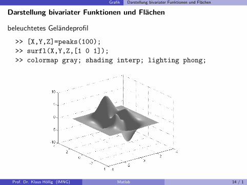
beleuchtetes Gelandeprofil
>> [X,Y,Z]=peaks(100);>> surfl(X,Y,Z,[1 0 1]);>> colormap gray; shading interp; lighting phong;
Prof. Dr. Klaus Hollig (IMNG) Matlab 14 / 1
Grafik Niveaulinien
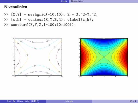
Niveaulinien
[c,h] = contour(X,Y,Z): Niveaulinen
contourf: Darstellung mit eingefarbten Bereichen
contour3: dreidimensionale Darstellung
optionale Anzahl n oder z-Werte v der Niveaulinien
Beschriftung:
clabel(c,h): z-Werte entlang der Niveaulinien
Prof. Dr. Klaus Hollig (IMNG) Matlab 15 / 1
Grafik Niveaulinien
Niveaulinien
>> [X,Y] = meshgrid(-10:10); Z = X.^2-Y.^2;>> [c,h] = contour(X,Y,Z,4); clabel(c,h);>> contourf(X,Y,Z,[-100:10:100]);
−60 −60
−60 −60
−20
−20
−20
−20
−20
−20
20
20
20
20
20
20
60
60
60
60
−10 −5 0 5 10−10
−8
−6
−4
−2
0
2
4
6
8
10
−10 −5 0 5 10−10
−8
−6
−4
−2
0
2
4
6
8
10
Prof. Dr. Klaus Hollig (IMNG) Matlab 16 / 1
Grafik Bilder und Animationen
Bilder und Animationen
Funktionen zur Bildverarbeitung:imread, imwrite Lesen und Schreiben von Grafikdateienimage Darstellung von Bildernimfinfo Ausgabe von Informationen zu einem Bild
Animationen:getframe Speichern von Animationsframesmovie Abspielen gespeicherter Framesim2frame, frame2im Konvertierung zwischen Bildern
und Movie-Framesmovie2avi Konvertiert Matlab-Movie in eine AVI-Dateiaviread Einlesen eines AVI-Films
Prof. Dr. Klaus Hollig (IMNG) Matlab 17 / 1
Grafik Bilder und Animationen
Bilder und Animationen
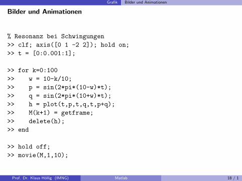
% Resonanz bei Schwingungen>> clf; axis([0 1 -2 2]); hold on;>> t = [0:0.001:1];
>> for k=0:100>> w = 10-k/10;>> p = sin(2*pi*(10-w)*t);>> q = sin(2*pi*(10+w)*t);>> h = plot(t,p,t,q,t,p+q);>> M(k+1) = getframe;>> delete(h);>> end
>> hold off;>> movie(M,1,10);
Prof. Dr. Klaus Hollig (IMNG) Matlab 18 / 1

Grafik Bilder und Animationen
Bilder und Animationen
Prof. Dr. Klaus Hollig (IMNG) Matlab 19 / 1

Grafik Speichern und Drucken von Grafiken
Speichern und Drucken von Grafiken
print Drucken und Speichern von Grafikenprint -d Format Dateiname Speichern im angegebenen Format
(z.B. bmp, epsc, jpeg, pdf, png, tiff)
Steuerung der Ausgabe
orient Einstellen der Papierorientierungprintdlg offnet Dialogfenster mit Druckeinstellungenpagesetupdlg offnet Dialogfenster mit Seiteneinstellungenprintpreview Vorschau der Druckausgabe
Prof. Dr. Klaus Hollig (IMNG) Matlab 20 / 1