MATLAB PrimerThird Edition

Kermit SigmonDepartment of Mathematics

University of Florida

Department of Mathematics • University of Florida • Gainesville, FL 32611sigmon@math.ufl.edu

Copyright c©1989, 1992, 1993 by Kermit Sigmon

Contents

Page

1. Accessing MATLAB . . . . . . . . . . . . . . . . . . . . . . . . . . . . . . . . . . . . . . . . . . . . . . . . . . . . . . . . . . . . . 1

2. Entering matrices . . . . . . . . . . . . . . . . . . . . . . . . . . . . . . . . . . . . . . . . . . . . . . . . . . . . . . . . . . . . . . . . 1

3. Matrix operations, array operations . . . . . . . . . . . . . . . . . . . . . . . . . . . . . . . . . . . . . . . . . . . . . . 2

4. Statements, expressions, variables; saving a session . . . . . . . . . . . . . . . . . . . . . . . . . . . . . . . 3

5. Matrix building functions . . . . . . . . . . . . . . . . . . . . . . . . . . . . . . . . . . . . . . . . . . . . . . . . . . . . . . . . 4

6. For, while, if — and relations . . . . . . . . . . . . . . . . . . . . . . . . . . . . . . . . . . . . . . . . . . . . . . . . . . . . 4

7. Scalar functions . . . . . . . . . . . . . . . . . . . . . . . . . . . . . . . . . . . . . . . . . . . . . . . . . . . . . . . . . . . . . . . . . 7

8. Vector functions . . . . . . . . . . . . . . . . . . . . . . . . . . . . . . . . . . . . . . . . . . . . . . . . . . . . . . . . . . . . . . . . . 7

9. Matrix functions . . . . . . . . . . . . . . . . . . . . . . . . . . . . . . . . . . . . . . . . . . . . . . . . . . . . . . . . . . . . . . . . . 7

10. Command line editing and recall . . . . . . . . . . . . . . . . . . . . . . . . . . . . . . . . . . . . . . . . . . . . . . . . . 8

11. Submatrices and colon notation . . . . . . . . . . . . . . . . . . . . . . . . . . . . . . . . . . . . . . . . . . . . . . . . . . 8

12. M-files: script files, function files . . . . . . . . . . . . . . . . . . . . . . . . . . . . . . . . . . . . . . . . . . . . . . . . . 9

13. Text strings, error messages, input . . . . . . . . . . . . . . . . . . . . . . . . . . . . . . . . . . . . . . . . . . . . . . 12

14. Managing M-files . . . . . . . . . . . . . . . . . . . . . . . . . . . . . . . . . . . . . . . . . . . . . . . . . . . . . . . . . . . . . . . 13

15. Comparing efficiency of algorithms: flops, tic, toc . . . . . . . . . . . . . . . . . . . . . . . . . . . . . . . 14

16. Output format . . . . . . . . . . . . . . . . . . . . . . . . . . . . . . . . . . . . . . . . . . . . . . . . . . . . . . . . . . . . . . . . . 14

17. Hard copy . . . . . . . . . . . . . . . . . . . . . . . . . . . . . . . . . . . . . . . . . . . . . . . . . . . . . . . . . . . . . . . . . . . . . . 15

18. Graphics . . . . . . . . . . . . . . . . . . . . . . . . . . . . . . . . . . . . . . . . . . . . . . . . . . . . . . . . . . . . . . . . . . . . . . . 15planar plots (15), hardcopy (17), 3-D line plots (18)mesh and surface plots (18), Handle Graphics (20)

19. Sparse matrix computations . . . . . . . . . . . . . . . . . . . . . . . . . . . . . . . . . . . . . . . . . . . . . . . . . . . . 20

20. Reference . . . . . . . . . . . . . . . . . . . . . . . . . . . . . . . . . . . . . . . . . . . . . . . . . . . . . . . . . . . . . . . . . . . . . . 22

iii

1. Accessing MATLAB.

On most systems, after logging in one can enter MATLAB with the system commandmatlab and exit MATLAB with the MATLAB command quit or exit. However, yourlocal installation may permit MATLAB to be accessed from a menu or by clicking an icon.

On systems permitting multiple processes, such as a Unix system or MS Windows,you will find it convenient, for reasons discussed in section 14, to keep both MATLABand your local editor active. If you are working on a platform which runs processes inmultiple windows, you will want to keep MATLAB active in one window and your localeditor active in another.

You should consult your instructor or your local computer center for details of the localinstallation.

2. Entering matrices.

MATLAB works with essentially only one kind of object—a rectangular numericalmatrix with possibly complex entries; all variables represent matrices. In some situations,1-by-1 matrices are interpreted as scalars and matrices with only one row or one columnare interpreted as vectors.

Matrices can be introduced into MATLAB in several different ways:

• Entered by an explicit list of elements,

• Generated by built-in statements and functions,

• Created in a diskfile with your local editor,

• Loaded from external data files or applications (see the User’s Guide).

For example, either of the statements

A = [1 2 3; 4 5 6; 7 8 9]

and

A = [

1 2 3

4 5 6

7 8 9 ]

creates the obvious 3-by-3 matrix and assigns it to a variable A. Try it. The elementswithin a row of a matrix may be separated by commas as well as a blank. When listing anumber in exponential form (e.g. 2.34e-9), blank spaces must be avoided.

MATLAB allows complex numbers in all its operations and functions. Two convenientways to enter complex matrices are:

A = [1 2;3 4] + i*[5 6;7 8]

A = [1+5i 2+6i;3+7i 4+8i]

When listing complex numbers (e.g. 2+6i) in a matrix, blank spaces must be avoided.Either i or j may be used as the imaginary unit. If, however, you use i and j as vari-ables and overwrite their values, you may generate a new imaginary unit with, say,ii = sqrt(-1).

1

Listing entries of a large matrix is best done in an ASCII file with your local editor,where errors can be easily corrected (see sections 12 and 14). The file should consist of arectangular array of just the numeric matrix entries. If this file is named, say, data.ext(where .ext is any extension), the MATLAB command load data.ext will read this fileto the variable data in your MATLAB workspace. This may also be done with a script file(see section 12).

The built-in functions rand, magic, and hilb, for example, provide an easy way tocreate matrices with which to experiment. The command rand(n) will create an n × nmatrix with randomly generated entries distributed uniformly between 0 and 1, whilerand(m,n) will create an m× n one. magic(n) will create an integral n× n matrix whichis a magic square (rows, columns, and diagonals have common sum); hilb(n) will createthe n× n Hilbert matrix, the king of ill-conditioned matrices (m and n denote, of course,positive integers). Matrices can also be generated with a for-loop (see section 6 below).

Individual matrix and vector entries can be referenced with indices inside parenthesesin the usual manner. For example, A(2, 3) denotes the entry in the second row, thirdcolumn of matrix A and x(3) denotes the third coordinate of vector x. Try it. A matrixor a vector will only accept positive integers as indices.

3. Matrix operations, array operations.

The following matrix operations are available in MATLAB:

+ addition− subtraction∗ multiplication power′ conjugate transpose\ left division/ right division

These matrix operations apply, of course, to scalars (1-by-1 matrices) as well. If the sizesof the matrices are incompatible for the matrix operation, an error message will result,except in the case of scalar-matrix operations (for addition, subtraction, and division aswell as for multiplication) in which case each entry of the matrix is operated on by thescalar.

The “matrix division” operations deserve special comment. If A is an invertible squarematrix and b is a compatible column, resp. row, vector, then

x = A\b is the solution of A ∗ x = b and, resp.,x = b/A is the solution of x ∗A = b.

In left division, if A is square, then it is factored using Gaussian elimination and thesefactors are used to solve A ∗ x = b. If A is not square, it is factored using Householderorthogonalization with column pivoting and the factors are used to solve the under- orover- determined system in the least squares sense. Right division is defined in terms ofleft division by b/A = (A′\b′)′.

2

Array operations.

The matrix operations of addition and subtraction already operate entry-wise but theother matrix operations given above do not—they are matrix operations. It is impor-tant to observe that these other operations, ∗, , \, and /, can be made to operateentry-wise by preceding them by a period. For example, either [1,2,3,4].*[1,2,3,4]

or [1,2,3,4]. 2 will yield [1,4,9,16]. Try it. This is particularly useful when usingMatlab graphics.

4. Statements, expressions, and variables; saving a session.

MATLAB is an expression language; the expressions you type are interpreted andevaluated. MATLAB statements are usually of the form

variable = expression, or simplyexpression

Expressions are usually composed from operators, functions, and variable names. Eval-uation of the expression produces a matrix, which is then displayed on the screen andassigned to the variable for future use. If the variable name and = sign are omitted, avariable ans (for answer) is automatically created to which the result is assigned.

A statement is normally terminated with the carriage return. However, a statement canbe continued to the next line with three or more periods followed by a carriage return. Onthe other hand, several statements can be placed on a single line if separated by commasor semicolons.

If the last character of a statement is a semicolon, the printing is suppressed, but theassignment is carried out. This is essential in suppressing unwanted printing of intermediateresults.

MATLAB is case-sensitive in the names of commands, functions, and variables. Forexample, solveUT is not the same as solveut.

The command who (or whos) will list the variables currently in the workspace. Avariable can be cleared from the workspace with the command clear variablename. Thecommand clear alone will clear all nonpermanent variables.

The permanent variable eps (epsilon) gives the machine unit roundoff—about 10−16 onmost machines. It is useful in specifying tolerences for convergence of iterative processes.

A runaway display or computation can be stopped on most machines without leavingMATLAB with CTRL-C (CTRL-BREAK on a PC).

Saving a session.

When one logs out or exits MATLAB all variables are lost. However, invoking thecommand save before exiting causes all variables to be written to a non-human-readablediskfile named matlab.mat. When one later reenters MATLAB, the command load willrestore the workspace to its former state.

3

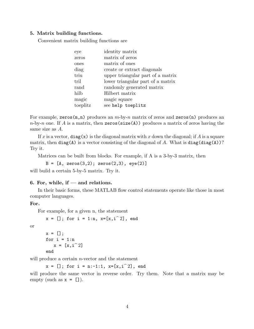
5. Matrix building functions.

Convenient matrix building functions are

eye identity matrixzeros matrix of zerosones matrix of onesdiag create or extract diagonalstriu upper triangular part of a matrixtril lower triangular part of a matrixrand randomly generated matrixhilb Hilbert matrixmagic magic squaretoeplitz see help toeplitz

For example, zeros(m,n) produces an m-by-n matrix of zeros and zeros(n) produces ann-by-n one. If A is a matrix, then zeros(size(A)) produces a matrix of zeros having thesame size as A.

If x is a vector, diag(x) is the diagonal matrix with x down the diagonal; if A is a squarematrix, then diag(A) is a vector consisting of the diagonal of A. What is diag(diag(A))?Try it.

Matrices can be built from blocks. For example, if A is a 3-by-3 matrix, then

B = [A, zeros(3,2); zeros(2,3), eye(2)]

will build a certain 5-by-5 matrix. Try it.

6. For, while, if — and relations.

In their basic forms, these MATLAB flow control statements operate like those in mostcomputer languages.

For.

For example, for a given n, the statement

x = []; for i = 1:n, x=[x,i 2], end

or

x = [];

for i = 1:n

x = [x,i 2]end

will produce a certain n-vector and the statement

x = []; for i = n:-1:1, x=[x,i 2], end

will produce the same vector in reverse order. Try them. Note that a matrix may beempty (such as x = []).

4

The statements

for i = 1:m

for j = 1:n

H(i, j) = 1/(i+j-1);

end

end

H

will produce and print to the screen the m-by-n hilbert matrix. The semicolon on theinner statement is essential to suppress printing of unwanted intermediate results whilethe last H displays the final result.

The for statement permits any matrix to be used instead of 1:n. The variable justconsecutively assumes the value of each column of the matrix. For example,

s = 0;

for c = A

s = s + sum(c);

end

computes the sum of all entries of the matrix A by adding its column sums (Of course,sum(sum(A)) does it more efficiently; see section 8). In fact, since 1:n = [1,2,3,. . . ,n],this column-by-column assigment is what occurs with “if i = 1:n,. . . ” (see section 11).

While.

The general form of a while loop is

while relationstatements

end

The statements will be repeatedly executed as long as the relation remains true. For exam-ple, for a given number a, the following will compute and display the smallest nonnegativeinteger n such that 2n ≥ a:

n = 0;

while 2 n < a

n = n + 1;

end

n

If.

The general form of a simple if statement is

if relationstatements

end

The statements will be executed only if the relation is true. Multiple branching is alsopossible, as is illustrated by

if n < 0

parity = 0;

5

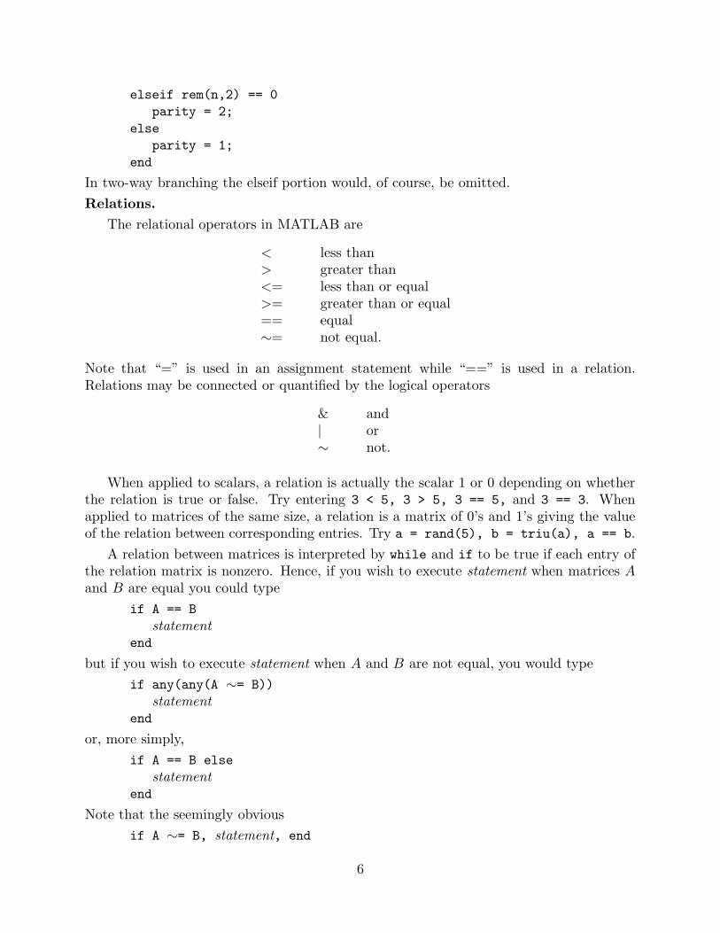
elseif rem(n,2) == 0

parity = 2;

else

parity = 1;

end

In two-way branching the elseif portion would, of course, be omitted.

Relations.

The relational operators in MATLAB are

< less than> greater than<= less than or equal>= greater than or equal== equal∼= not equal.

Note that “=” is used in an assignment statement while “==” is used in a relation.Relations may be connected or quantified by the logical operators

& and| or∼ not.

When applied to scalars, a relation is actually the scalar 1 or 0 depending on whetherthe relation is true or false. Try entering 3 < 5, 3 > 5, 3 == 5, and 3 == 3. Whenapplied to matrices of the same size, a relation is a matrix of 0’s and 1’s giving the valueof the relation between corresponding entries. Try a = rand(5), b = triu(a), a == b.

A relation between matrices is interpreted by while and if to be true if each entry ofthe relation matrix is nonzero. Hence, if you wish to execute statement when matrices Aand B are equal you could type

if A == B

statementend

but if you wish to execute statement when A and B are not equal, you would type

if any(any(A ∼= B))

statementend

or, more simply,

if A == B else

statementend

Note that the seemingly obvious

if A ∼= B, statement, end

6

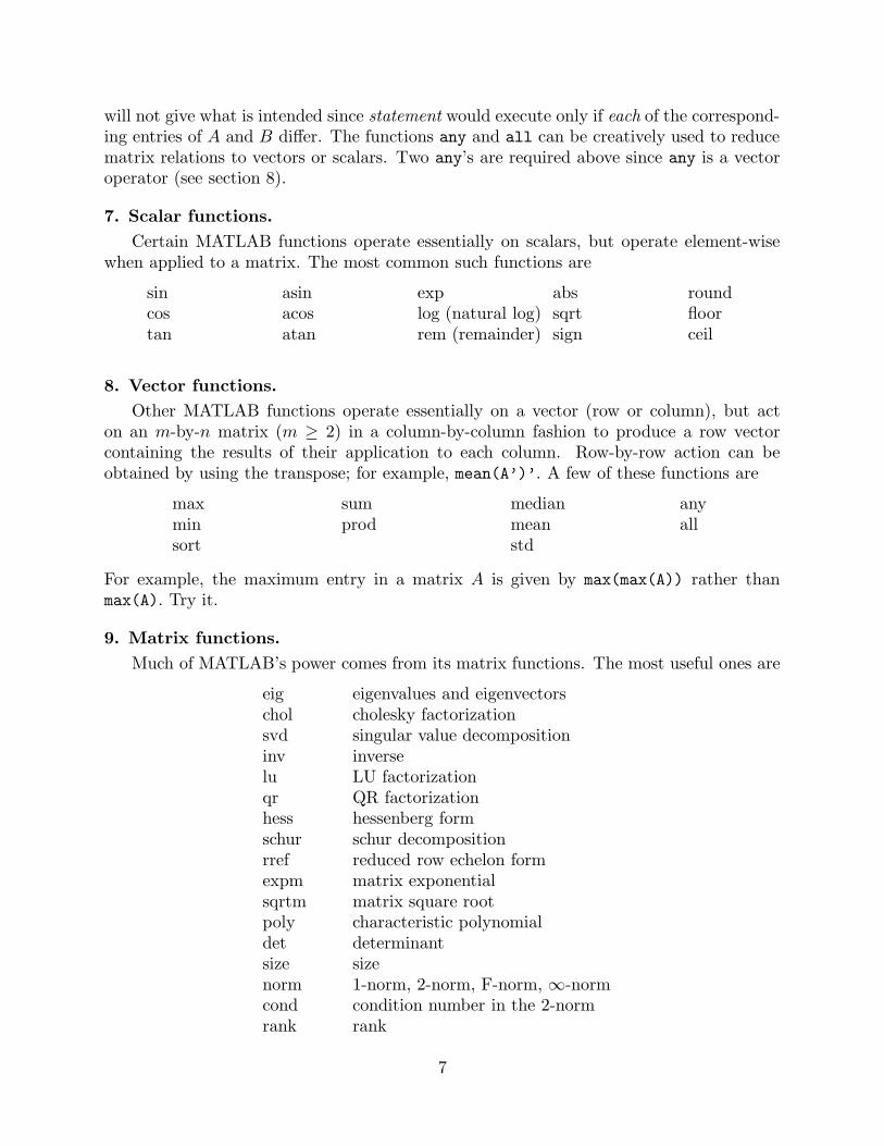
will not give what is intended since statement would execute only if each of the correspond-ing entries of A and B differ. The functions any and all can be creatively used to reducematrix relations to vectors or scalars. Two any’s are required above since any is a vectoroperator (see section 8).

7. Scalar functions.

Certain MATLAB functions operate essentially on scalars, but operate element-wisewhen applied to a matrix. The most common such functions are

sin asin exp abs roundcos acos log (natural log) sqrt floortan atan rem (remainder) sign ceil

8. Vector functions.

Other MATLAB functions operate essentially on a vector (row or column), but acton an m-by-n matrix (m ≥ 2) in a column-by-column fashion to produce a row vectorcontaining the results of their application to each column. Row-by-row action can beobtained by using the transpose; for example, mean(A’)’. A few of these functions are

max sum median anymin prod mean allsort std

For example, the maximum entry in a matrix A is given by max(max(A)) rather thanmax(A). Try it.

9. Matrix functions.

Much of MATLAB’s power comes from its matrix functions. The most useful ones are

eig eigenvalues and eigenvectorschol cholesky factorizationsvd singular value decompositioninv inverselu LU factorizationqr QR factorizationhess hessenberg formschur schur decompositionrref reduced row echelon formexpm matrix exponentialsqrtm matrix square rootpoly characteristic polynomialdet determinantsize sizenorm 1-norm, 2-norm, F-norm, ∞-normcond condition number in the 2-normrank rank

7

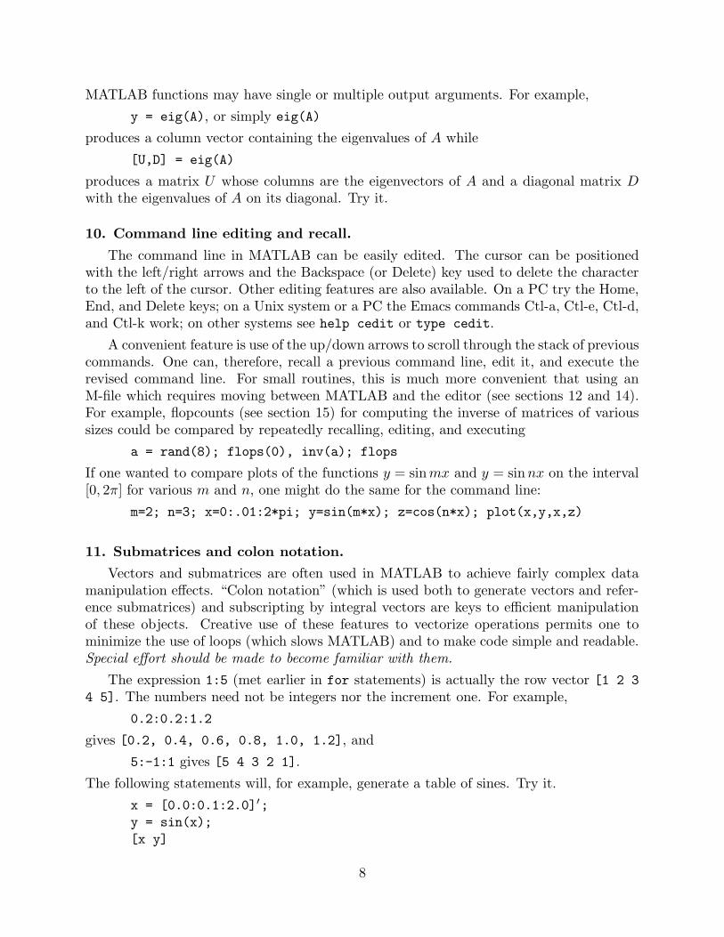
MATLAB functions may have single or multiple output arguments. For example,

y = eig(A), or simply eig(A)

produces a column vector containing the eigenvalues of A while

[U,D] = eig(A)

produces a matrix U whose columns are the eigenvectors of A and a diagonal matrix Dwith the eigenvalues of A on its diagonal. Try it.

10. Command line editing and recall.

The command line in MATLAB can be easily edited. The cursor can be positionedwith the left/right arrows and the Backspace (or Delete) key used to delete the characterto the left of the cursor. Other editing features are also available. On a PC try the Home,End, and Delete keys; on a Unix system or a PC the Emacs commands Ctl-a, Ctl-e, Ctl-d,and Ctl-k work; on other systems see help cedit or type cedit.

A convenient feature is use of the up/down arrows to scroll through the stack of previouscommands. One can, therefore, recall a previous command line, edit it, and execute therevised command line. For small routines, this is much more convenient that using anM-file which requires moving between MATLAB and the editor (see sections 12 and 14).For example, flopcounts (see section 15) for computing the inverse of matrices of varioussizes could be compared by repeatedly recalling, editing, and executing

a = rand(8); flops(0), inv(a); flops

If one wanted to compare plots of the functions y = sinmx and y = sinnx on the interval[0, 2π] for various m and n, one might do the same for the command line:

m=2; n=3; x=0:.01:2*pi; y=sin(m*x); z=cos(n*x); plot(x,y,x,z)

11. Submatrices and colon notation.

Vectors and submatrices are often used in MATLAB to achieve fairly complex datamanipulation effects. “Colon notation” (which is used both to generate vectors and refer-ence submatrices) and subscripting by integral vectors are keys to efficient manipulationof these objects. Creative use of these features to vectorize operations permits one tominimize the use of loops (which slows MATLAB) and to make code simple and readable.Special effort should be made to become familiar with them.

The expression 1:5 (met earlier in for statements) is actually the row vector [1 2 3

4 5]. The numbers need not be integers nor the increment one. For example,

0.2:0.2:1.2

gives [0.2, 0.4, 0.6, 0.8, 1.0, 1.2], and

5:-1:1 gives [5 4 3 2 1].

The following statements will, for example, generate a table of sines. Try it.

x = [0.0:0.1:2.0]′;y = sin(x);

[x y]

8

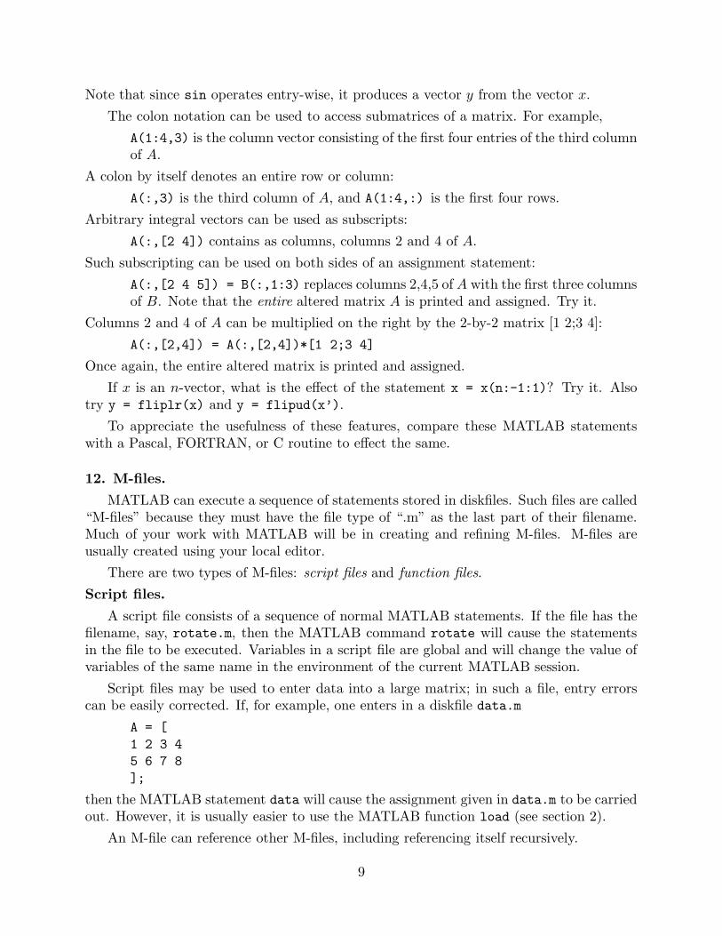
Note that since sin operates entry-wise, it produces a vector y from the vector x.

The colon notation can be used to access submatrices of a matrix. For example,

A(1:4,3) is the column vector consisting of the first four entries of the third columnof A.

A colon by itself denotes an entire row or column:

A(:,3) is the third column of A, and A(1:4,:) is the first four rows.

Arbitrary integral vectors can be used as subscripts:

A(:,[2 4]) contains as columns, columns 2 and 4 of A.

Such subscripting can be used on both sides of an assignment statement:

A(:,[2 4 5]) = B(:,1:3) replaces columns 2,4,5 of A with the first three columnsof B. Note that the entire altered matrix A is printed and assigned. Try it.

Columns 2 and 4 of A can be multiplied on the right by the 2-by-2 matrix [1 2;3 4]:

A(:,[2,4]) = A(:,[2,4])*[1 2;3 4]

Once again, the entire altered matrix is printed and assigned.

If x is an n-vector, what is the effect of the statement x = x(n:-1:1)? Try it. Alsotry y = fliplr(x) and y = flipud(x’).

To appreciate the usefulness of these features, compare these MATLAB statementswith a Pascal, FORTRAN, or C routine to effect the same.

12. M-files.

MATLAB can execute a sequence of statements stored in diskfiles. Such files are called“M-files” because they must have the file type of “.m” as the last part of their filename.Much of your work with MATLAB will be in creating and refining M-files. M-files areusually created using your local editor.

There are two types of M-files: script files and function files.

Script files.

A script file consists of a sequence of normal MATLAB statements. If the file has thefilename, say, rotate.m, then the MATLAB command rotate will cause the statementsin the file to be executed. Variables in a script file are global and will change the value ofvariables of the same name in the environment of the current MATLAB session.

Script files may be used to enter data into a large matrix; in such a file, entry errorscan be easily corrected. If, for example, one enters in a diskfile data.m

A = [

1 2 3 4

5 6 7 8

];

then the MATLAB statement data will cause the assignment given in data.m to be carriedout. However, it is usually easier to use the MATLAB function load (see section 2).

An M-file can reference other M-files, including referencing itself recursively.

9

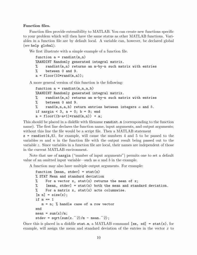
Function files.

Function files provide extensibility to MATLAB. You can create new functions specificto your problem which will then have the same status as other MATLAB functions. Vari-ables in a function file are by default local. A variable can, however, be declared global(see help global).

We first illustrate with a simple example of a function file.

function a = randint(m,n)

%RANDINT Randomly generated integral matrix.

% randint(m,n) returns an m-by-n such matrix with entries

% between 0 and 9.

a = floor(10*rand(m,n));

A more general version of this function is the following:

function a = randint(m,n,a,b)

%RANDINT Randomly generated integral matrix.

% randint(m,n) returns an m-by-n such matrix with entries

% between 0 and 9.

% rand(m,n,a,b) return entries between integers a and b.if nargin < 3, a = 0; b = 9; end

a = floor((b-a+1)*rand(m,n)) + a;

This should be placed in a diskfile with filename randint.m (corresponding to the functionname). The first line declares the function name, input arguments, and output arguments;without this line the file would be a script file. Then a MATLAB statementz = randint(4,5), for example, will cause the numbers 4 and 5 to be passed to thevariables m and n in the function file with the output result being passed out to thevariable z. Since variables in a function file are local, their names are independent of thosein the current MATLAB environment.

Note that use of nargin (“number of input arguments”) permits one to set a defaultvalue of an omitted input variable—such as a and b in the example.

A function may also have multiple output arguments. For example:

function [mean, stdev] = stat(x)

% STAT Mean and standard deviation

% For a vector x, stat(x) returns the mean of x;

% [mean, stdev] = stat(x) both the mean and standard deviation.

% For a matrix x, stat(x) acts columnwise.

[m n] = size(x);

if m == 1

m = n; % handle case of a row vector

end

mean = sum(x)/m;

stdev = sqrt(sum(x. 2)/m - mean. 2);

Once this is placed in a diskfile stat.m, a MATLAB command [xm, xd] = stat(x), forexample, will assign the mean and standard deviation of the entries in the vector x to

10

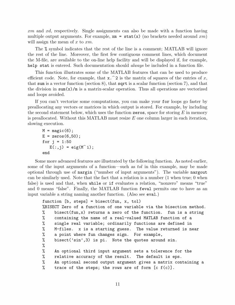
xm and xd, respectively. Single assignments can also be made with a function havingmultiple output arguments. For example, xm = stat(x) (no brackets needed around xm)will assign the mean of x to xm.

The % symbol indicates that the rest of the line is a comment; MATLAB will ignorethe rest of the line. Moreover, the first few contiguous comment lines, which documentthe M-file, are available to the on-line help facility and will be displayed if, for example,help stat is entered. Such documentation should always be included in a function file.

This function illustrates some of the MATLAB features that can be used to produceefficient code. Note, for example, that x. 2 is the matrix of squares of the entries of x,that sum is a vector function (section 8), that sqrt is a scalar function (section 7), and thatthe division in sum(x)/m is a matrix-scalar operation. Thus all operations are vectorizedand loops avoided.

If you can’t vectorize some computations, you can make your for loops go faster bypreallocating any vectors or matrices in which output is stored. For example, by includingthe second statement below, which uses the function zeros, space for storing E in memoryis preallocated. Without this MATLAB must resize E one column larger in each iteration,slowing execution.

M = magic(6);

E = zeros(6,50);

for j = 1:50

E(:,j) = eig(M i);end

Some more advanced features are illustrated by the following function. As noted earlier,some of the input arguments of a function—such as tol in this example, may be madeoptional through use of nargin (“number of input arguments”). The variable nargout

can be similarly used. Note that the fact that a relation is a number (1 when true; 0 whenfalse) is used and that, when while or if evaluates a relation, “nonzero” means “true”and 0 means “false”. Finally, the MATLAB function feval permits one to have as aninput variable a string naming another function. (Also see eval.)

function [b, steps] = bisect(fun, x, tol)

%BISECT Zero of a function of one variable via the bisection method.

% bisect(fun,x) returns a zero of the function. fun is a string

% containing the name of a real-valued MATLAB function of a

% single real variable; ordinarily functions are defined in

% M-files. x is a starting guess. The value returned is near

% a point where fun changes sign. For example,

% bisect(’sin’,3) is pi. Note the quotes around sin.

%

% An optional third input argument sets a tolerence for the

% relative accuracy of the result. The default is eps.

% An optional second output argument gives a matrix containing a

% trace of the steps; the rows are of form [c f(c)].

11

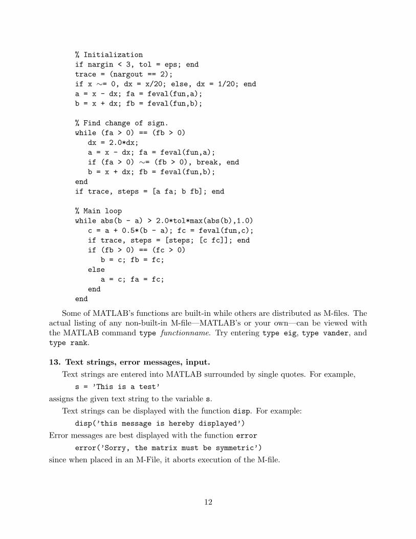
% Initialization

if nargin < 3, tol = eps; end

trace = (nargout == 2);

if x ∼= 0, dx = x/20; else, dx = 1/20; end

a = x - dx; fa = feval(fun,a);

b = x + dx; fb = feval(fun,b);

% Find change of sign.

while (fa > 0) == (fb > 0)

dx = 2.0*dx;

a = x - dx; fa = feval(fun,a);

if (fa > 0) ∼= (fb > 0), break, end

b = x + dx; fb = feval(fun,b);

end

if trace, steps = [a fa; b fb]; end

% Main loop

while abs(b - a) > 2.0*tol*max(abs(b),1.0)

c = a + 0.5*(b - a); fc = feval(fun,c);

if trace, steps = [steps; [c fc]]; end

if (fb > 0) == (fc > 0)

b = c; fb = fc;

else

a = c; fa = fc;

end

end

Some of MATLAB’s functions are built-in while others are distributed as M-files. Theactual listing of any non-built-in M-file—MATLAB’s or your own—can be viewed withthe MATLAB command type functionname. Try entering type eig, type vander, andtype rank.

13. Text strings, error messages, input.

Text strings are entered into MATLAB surrounded by single quotes. For example,

s = ’This is a test’

assigns the given text string to the variable s.

Text strings can be displayed with the function disp. For example:

disp(’this message is hereby displayed’)

Error messages are best displayed with the function error

error(’Sorry, the matrix must be symmetric’)

since when placed in an M-File, it aborts execution of the M-file.

12

In an M-file the user can be prompted to interactively enter input data with the functioninput. When, for example, the statement

iter = input(’Enter the number of iterations: ’)

is encountered, the prompt message is displayed and execution pauses while the user keysin the input data. Upon pressing the return key, the data is assigned to the variable iter

and execution resumes.

14. Managing M-files.

While using MATLAB one frequently wishes to create or edit an M-file with the localeditor and then return to MATLAB. One wishes to keep MATLAB active while editing afile since otherwise all variables would be lost upon exiting.

This can be easily done using the !-feature. If, while in MATLAB, you precede it withan !, any system command—such as those for editing, printing, or copying a file—can beexecuted without exiting MATLAB. If, for example, the system command ed accesses youreditor, the MATLAB command

>> !ed rotate.m

will let you edit the file named rotate.m using your local editor. Upon leaving the editor,you will be returned to MATLAB just where you left it.

However, as noted in section 1, on systems permitting multiple processes, such as onerunning Unix or MS Windows, it may be preferable to keep both MATLAB and your localeditor active, keeping one process suspended while working in the other. If these processescan be run in multiple windows, you will want to keep MATLAB active in one windowand your editor active in another.

You should consult your instructor or your local computing center for details of thelocal installation.

Many debugging tools are available. See help dbtype or the list of functions in thelast section.

When in MATLAB, the command pwd will return the name of the present workingdirectory and cd can be used to change the working directory. Either dir or ls will listthe contents of the working directory while the command what lists only the M-files in thedirectory. The MATLAB commands delete and type can be used to delete a diskfile andprint an M-file to the screen, respectively. While these commands may duplicate systemcommands, they avoid the use of an !. You may enjoy entering the command why a fewtimes.

M-files must be in a directory accessible to MATLAB. M-files in the present work-ing directory are always accessible. On most mainframe or workstation network installa-tions, personal M-files which are stored in a subdirectory of one’s home directory namedmatlab will be accessible to MATLAB from any directory in which one is working. Thecurrent list of directories in MATLAB’s search path is obtained by the command path.This command can also be used to add or delete directories from the search path. Seehelp path.

13

15. Comparing efficiency of algorithms: flops, tic and toc.

Two measures of the efficiency of an algorithm are the number of floating point oper-ations (flops) performed and the elapsed time.

The MATLAB function flops keeps a running total of the flops performed. Thecommand flops(0) (not flops = 0!) will reset flops to 0. Hence, entering flops(0)

immediately before executing an algorithm and flops immediately after gives the flopcount for the algorithm. For example, the number of flops required to solve a given linearsystem via Gaussian elimination can be obtained with:

flops(0), x = A\b; flops

The elapsed time (in seconds) can be obtained with the stopwatch timers tic and toc;tic starts the timer and toc returns the elapsed time. Hence, the commands

tic, any statement, toc

will return the elapsed time for execution of the statement. The elapsed time for solvingthe linear system above can be obtained, for example, with:

tic, x = A\b; toc

You may wish to compare this time—and flop count—with that for solving the systemusing x = inv(A)*b;. Try it.

It should be noted that, on timesharing machines, elapsed time may not be a reliablemeasure of the efficiency of an algorithm since the rate of execution depends on how busythe computer is at the time.

16. Output format.

While all computations in MATLAB are performed in double precision, the format ofthe displayed output can be controlled by the following commands.

format short fixed point with 4 decimal places (the default)format long fixed point with 14 decimal placesformat short e scientific notation with 4 decimal placesformat long e scientific notation with 15 decimal placesformat rat approximation by ratio of small integersformat hex hexadecimal formatformat bank fixed dollars and centsformat + +, -, blank

Once invoked, the chosen format remains in effect until changed.

The command format compact will suppress most blank lines allowing more infor-mation to be placed on the screen or page. The command format loose returns to thenon-compact format. These commands are independent of the other format commands.

14

17. Hardcopy.

Hardcopy is most easily obtained with the diary command. The command

diary filename

causes what appears subsequently on the screen (except graphics) to be written to thenamed diskfile (if the filename is omitted it will be written to a default file named diary)until one gives the command diary off; the command diary on will cause writing tothe file to resume, etc. When finished, you can edit the file as desired and print it out onthe local system. The !-feature (see section 14) will permit you to edit and print the filewithout leaving MATLAB.

18. Graphics.

MATLAB can produce planar plots of curves, 3-D plots of curves, 3-D mesh surfaceplots, and 3-D faceted surface plots. The primary commands for these facilities are plot,

plot3, mesh, and surf, respectively. An introduction to each of these is given below.

To preview some of these capabilities, enter the command demo and select some of thegraphics options.

Planar plots.

The plot command creates linear x-y plots; if x and y are vectors of the same length,the command plot(x,y) opens a graphics window and draws an x-y plot of the elementsof x versus the elements of y. You can, for example, draw the graph of the sine functionover the interval -4 to 4 with the following commands:

x = -4:.01:4; y = sin(x); plot(x,y)

Try it. The vector x is a partition of the domain with meshsize 0.01 while y is a vectorgiving the values of sine at the nodes of this partition (recall that sin operates entrywise).

You will usually want to keep the current graphics window (“figure”) exposed—butmoved to the side—and the command window active.

One can have several graphics figures, one of which will at any time be the designated“current” figure where graphs from subsequent plotting commands will be placed. If, forexample, figure 1 is the current figure, then the command figure(2) (or simply figure)will open a second figure (if necessary) and make it the current figure. The commandfigure(1) will then expose figure 1 and make it again the current figure. The commandgcf will return the number of the current figure.

As a second example, you can draw the graph of y = e−x2

over the interval -1.5 to 1.5as follows:

x = -1.5:.01:1.5; y = exp(-x. 2); plot(x,y)

Note that one must precede by a period to ensure that it operates entrywise (see section3).

MATLAB supplies a function fplot to easily and efficiently plot the graph of a function.For example, to plot the graph of the function above, one can first define the function inan M-file called, say, expnormal.m containing

15

function y = expnormal(x)

y = exp(-x. 2);Then the command

fplot(’expnormal’, [-1.5,1.5])

will produce the graph. Try it.

Plots of parametrically defined curves can also be made. Try, for example,

t=0:.001:2*pi; x=cos(3*t); y=sin(2*t); plot(x,y)

The graphs can be given titles, axes labeled, and text placed within the graph withthe following commands which take a string as an argument.

title graph titlexlabel x-axis labelylabel y-axis labelgtext place text on the graph using the mousetext position text at specified coordinates

For example, the command

title(’Best Least Squares Fit’)

gives a graph a title. The command gtext(’The Spot’) allows one to interactively placethe designated text on the current graph by placing the mouse pointer at the desiredposition and clicking the mouse. To place text in a graph at designated coordinates, onewould use the command text (see help text).

The command grid will place grid lines on the current graph.

By default, the axes are auto-scaled. This can be overridden by the command axis.Some features of axis are:

axis([xmin,xmax,ymin,ymax]) set axis scaling to prescribed limitsaxis(axis) freezes scaling for subsequent graphsaxis auto returns to auto-scalingv = axis returns vector v showing current scalingaxis square same scale on both axesaxis equal same scale and tic marks on both axesaxis off turns off axis scaling and tic marksaxis on turns on axis scaling and tic marks

The axis command should be given after the plot command.

Two ways to make multiple plots on a single graph are illustrated by

x=0:.01:2*pi;y1=sin(x);y2=sin(2*x);y3=sin(4*x);plot(x,y1,x,y2,x,y3)

and by forming a matrix Y containing the functional values as columns

x=0:.01:2*pi; Y=[sin(x)’, sin(2*x)’, sin(4*x)’]; plot(x,Y)

Another way is with hold. The command hold on freezes the current graphics screen sothat subsequent plots are superimposed on it. The axes may, however, become rescaled.Entering hold off releases the “hold.”

16

One can override the default linetypes, pointtypes and colors. For example,

x=0:.01:2*pi; y1=sin(x); y2=sin(2*x); y3=sin(4*x);

plot(x,y1,’--’,x,y2,’:’,x,y3,’+’)

renders a dashed line and dotted line for the first two graphs while for the third the symbol+ is placed at each node. The line- and mark-types are

Linetypes: solid (-), dashed (--). dotted (:), dashdot (-.)Marktypes: point (.), plus (+), star (*), circle (o), x-mark (x)

Colors can be specified for the line- and mark-types.

Colors: yellow (y), magenta (m), cyan (c), red (r)green (g), blue (b), white (w), black (k)

For example, plot(x,y,’r--’) plots a red dashed line.

The command subplot can be used to partition the screen so that several small plotscan be placed in one figure. See help subplot.

Other specialized 2-D plotting functions you may wish to explore via help are:

polar, bar, hist, quiver, compass, feather, rose, stairs, fill

Graphics hardcopy

A hardcopy of the current graphics figure can be most easily obtained with the MAT-LAB command print. Entered by itself, it will send a high-resolution copy of the currentgraphics figure to the default printer.

The printopt M-file is used to specify the default setting used by the print command.If desired, one can change the defaults by editing this file (see help printopt).

The command print filename saves the current graphics figure to the designatedfilename in the default file format. If filename has no extension, then an appropriateextension such as .ps, .eps, or .jet is appended. If, for example, PostScript is thedefault file format, then

print lissajous

will create a PostScript file lissajous.ps of the current graphics figure which can subse-quently be printed using the system print command. If filename already exists, it will beoverwritten unless you use the -append option. The command

print -append lissajous

will append the (hopefully different) current graphics figure to the existing filelissajous.ps. In this way one can save several graphics figures in a single file.

The default settings can, of course, be overwritten. For example,

print -deps -f3 saddle

will save to an Encapsulated PostScript file saddle.eps the graphics figure 3 — even if itis not the current figure.

17

3-D line plots.

Completely analogous to plot in two dimensions, the command plot3 produces curvesin three dimensional space. If x, y, and z are three vectors of the same size, then thecommand plot3(x,y,z) will produce a perspective plot of the piecewise linear curve in3-space passing through the points whose coordinates are the respective elements of x, y,and z. These vectors are usually defined parametrically. For example,

t=.01:.01:20*pi; x=cos(t); y=sin(t); z=t. 3; plot3(x,y,z)

will produce a helix which is compressed near the x-y plane (a “slinky”). Try it.

Just as for planar plots, a title and axis labels (including zlabel) can be added. Thefeatures of axis command described there also hold for 3-D plots; setting the axis scalingto prescribed limits will, of course, now require a 6-vector.

3-D mesh and surface plots.

Three dimensional wire mesh surface plots are drawn with the command mesh. Thecommand mesh(z) creates a three-dimensional perspective plot of the elements of thematrix z. The mesh surface is defined by the z-coordinates of points above a rectangulargrid in the x-y plane. Try mesh(eye(10)).

Similarly, three dimensional faceted surface plots are drawn with the command surf.Try surf(eye(10)).

To draw the graph of a function z = f(x, y) over a rectangle, one first defines vectorsxx and yy which give partitions of the sides of the rectangle. With the function meshgrid

one then creates a matrix x, each row of which equals xx and whose column length is thelength of yy, and similarly a matrix y, each column of which equals yy, as follows:

[x,y] = meshgrid(xx,yy);

One then computes a matrix z, obtained by evaluating f entrywise over the matrices xand y, to which mesh or surf can be applied.

You can, for example, draw the graph of z = e−x2−y2

over the square [−2, 2]× [−2, 2]as follows (try it):

xx = -2:.2:2;

yy = xx;

[x,y] = meshgrid(xx,yy);

z = exp(-x. 2 - y. 2);mesh(z)

One could, of course, replace the first three lines of the preceding with

[x,y] = meshgrid(-2:.2:2, -2:.2:2);

Try this plot with surf instead of mesh.

As noted above, the features of the axis command described in the section on planarplots also hold for 3-D plots as do the commands for titles, axes labelling and the commandhold.

The color shading of surfaces is set by the shading command. There are three settingsfor shading: faceted (default), interpolated, and flat. These are set by the commands

18

shading faceted, shading interp, or shading flat

Note that on surfaces produced by surf, the settings interpolated and flat removethe superimposed mesh lines. Experiment with various shadings on the surface producedabove. The command shading (as well as colormap and view below) should be enteredafter the surf command.

The color profile of a surface is controlled by the colormap command. Available pre-defined colormaps include:

hsv (default), hot, cool, jet, pink, copper, flag, gray, bone

The command colormap(cool) will, for example, set a certain color profile for the currentfigure. Experiment with various colormaps on the surface produced above.

The command view can be used to specify in spherical or cartesian coordinates theviewpoint from which the 3-D object is to be viewed. See help view.

The MATLAB function peaks generates an interesting surface on which to experimentwith shading, colormap, and view.

Plots of parametrically defined surfaces can also be made. The MATLAB functionssphere and cylinder will generate such plots of the named surfaces. (See type sphere

and type cylinder.) The following is an example of a similar function which generates aplot of a torus.

function [x,y,z] = torus(r,n,a)

%TORUS Generate a torus

% torus(r,n,a) generates a plot of a torus with central

% radius a and lateral radius r. n controls the number

% of facets on the surface. These input variables are optional

% with defaults r = 0.5, n = 30, a = 1.

%

% [x,y,z] = torus(r,n,a) generates three (n+1)-by-(n+1)

% matrices so that surf(x,y,z) will produce the torus.

%

% See also SPHERE, CYLINDER

if nargin < 3, a = 1; end

if nargin < 2, n = 30; end

if nargin < 1, r = 0.5; end

theta = pi*(0:2:2*n)/n;

phi = 2*pi*(0:2:n)’/n;

xx = (a + r*cos(phi))*cos(theta);

yy = (a + r*cos(phi))*sin(theta);

zz = r*sin(phi)*ones(size(theta));

if nargout == 0

surf(xx,yy,zz)

ar = (a + r)/sqrt(2);

axis([-ar,ar,-ar,ar,-ar,ar])

else

19

x = xx; y = yy; z = zz;

end

Other 3-D plotting functions you may wish to explore via help are:

meshz, surfc, surfl, contour, pcolor

Handle Graphics.

Beyond those described above, MATLAB’s graphics system provides low level functionswhich permit one to control virtually all aspects of the graphics environment to producesophisticated plots. Enter the command set(1) and gca,set(ans) to see some of theproperties of figure 1 which one can control. This system is called Handle Graphics, forwhich one is referred to the MATLAB User’s Guide.

19. Sparse Matrix Computations.

In performing matrix computations, MATLAB normally assumes that a matrix isdense; that is, any entry in a matrix may be nonzero. If, however, a matrix containssufficiently many zero entries, computation time could be reduced by avoiding arithmeticoperations on zero entries and less memory could be required by storing only the nonzeroentries of the matrix. This increase in efficiency in time and storage can make feasiblethe solution of significantly larger problems than would otherwise be possible. MATLABprovides the capability to take advantage of the sparsity of matrices.

Matlab has two storage modes, full and sparse, with full the default. The functionsfull and sparse convert between the two modes. For a matrix A, full or sparse, nnz(A)returns the number of nonzero elements in A.

A sparse matrix is stored as a linear array of its nonzero elements along with their rowand column indices. If a full tridiagonal matrix F is created via, say,

F = floor(10*rand(6)); F = triu(tril(F,1),-1);

then the statement S = sparse(F) will convert F to sparse mode. Try it. Note that theoutput lists the nonzero entries in column major order along with their row and columnindices. The statement F = full(S) restores S to full storage mode. One can check thestorage mode of a matrix A with the command issparse(A).

A sparse matrix is, of course, usually generated directly rather than by applying thefunction sparse to a full matrix. A sparse banded matrix can be easily created via thefunction spdiags by specifying diagonals. For example, a familiar sparse tridiagonal matrixis created by

m = 6; n = 6; e = ones(n,1); d = -2*e;

T = spdiags([e,d,e],[-1,0,1],m,n)

Try it. The integral vector [-1,0,1] specifies in which diagonals the columns of [e,d,e] shouldbe placed (use full(T) to view). Experiment with other values of m and n and, say, [-3,0,2]instead of [-1,0,1]. See help spdiags for further features of spdiags.

20

The sparse analogs of eye, zeros, ones, and randn for full matrices are, respectively,

speye, sparse, spones, sprandn

The latter two take a matrix argument and replace only the nonzero entries with onesand normally distributed random numbers, respectively. randn also permits the sparsitystructure to be randomized. The command sparse(m,n) creates a sparse zero matrix.

The versatile function sparse permits creation of a sparse matrix via listing its nonzeroentries. Try, for example,

i = [1 2 3 4 4 4]; j = [1 2 3 1 2 3]; s = [5 6 7 8 9 10];

S = sparse(i,j,s,4,3), full(S)

In general, if the vector s lists the nonzero entries of S and the integral vectors i and j listtheir corresponding row and column indices, then

sparse(i,j,s,m,n)

will create the desired sparse m× n matrix S. As another example try

n = 6; e = floor(10*rand(n-1,1)); E = sparse(2:n,1:n-1,e,n,n)

The arithmetic operations and most MATLAB functions can be applied independentof storage mode. The storage mode of the result? Operations on full matrices always givefull results. Selected other results are (S=sparse, F=full):

Sparse: S+S, S*S, S.*S, S.*F, S n, S. n, S\SFull: S+F, S*F, S\F, F\SSparse: inv(S), chol(S), lu(S), diag(S), max(S), sum(S)

For sparse S, eig(S) is full if S is symmetric but undefined if S is unsymmetric; svd

requires a full argument. A matrix built from blocks, such as [A,B;C,D], is sparse if anyconstituent block is sparse.

You may wish to compare, for the two storage modes, the efficiency of solving a tridi-agonal system of equations for, say, n = 20, 50, 500, 1000 by entering, recalling and editingthe following two command lines:

n=20;e=ones(n,1);d=-2*e; T=spdiags([e,d,e],[-1,0,1],n,n); A=full(T);

b=ones(n,1);s=sparse(b);tic,T\s;sparsetime=toc, tic,A\b;fulltime=toc

21