matlab programming
TRANSCRIPT

Mohamed Abd Elhay


o MATLAB Application & usage
o MATLAB Environment
o MATLAB Variables
o MATLAB Operations.
o MATLAB Built-in Fun.
o MATLAB Scripts.

MATLAB stands for matrix laboratory.
o High-performance language for
technical computing.
o Integrates computation,
visualization, and programming in
an easy-to-use environment where
problems and solutions are
expressed in familiar mathematical
notation.

o Math and computation
o Algorithm development
o Data acquisition
o Modeling, simulation, and prototyping
o Data analysis, exploration, and visualization
o Scientific and engineering graphics
o Application development, including
graphical user interface building
The MATLAB Application:

The MATLAB system have five main parts:
1. Development Environment.
2. The MATLAB Mathematical Function Library.
3. The MATLAB Language.
4. Graphics.
5. The MATLAB Application Program Interface (API).
Code Generation
Blocksets
PC-based real-time systems
Stateflow Stateflow Stateflow Toolboxes
DAQ cards Instruments
Databases and files Financial Datafeeds
Desktop Applications Automated Reports

Statistics Statistics Toolbox o Contains about 250 functions and GUI’s for:
generating random numbers, probability
distributions, hypothesis Testing, statistical
plots and covers basic statistical functionality
Signal Processing Toolbox o An environment for signal analysis
waveform generation, statistical signal
processing, and spectral analysis
o Useful for designing filters in conjunction with
the image
processing toolbox
Signal Processing

Neural Network Toolbox o GUI for creating, training, and simulating
neural networks.
o It has support for the most commonly used
supervised
Optimization Toolbox o Includes standard algorithms for optimization
o Including minimax, goal attainment, and semi-
infinite minimization problems
Neural Networks
Optimization

Curve Fitting Toolbox o Allows you to develop custom linear and
nonlinear models in a graphical user interface.
o Calculates fits, residuals, confidence intervals,
first derivative and integral of the fit.
Another Tool boxes : o Communications Toolbox
o Control System Toolbox
o Data Acquisition Toolbox
o Database Toolbox
o Image Processing Toolbox
o Filter Design Toolbox
o Financial Toolbox
o Fixed-Point Toolbox
o Fuzzy Logic Toolbox

11/14
o Simulink is a graphical, “drag and drop” environment for building
simple and complex signal and system dynamic simulations.
o It allows users to concentrate on the structure of the problem, rather
than having to worry (too much) about a programming language.
o The parameters of each signal and system block is configured by the
user (right click on block)
o Signals and systems are simulated over a particular time.
vs, v
c
t
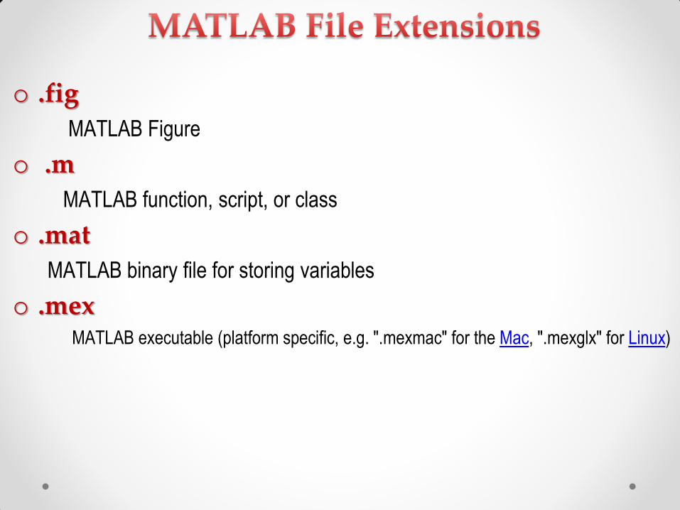
o .fig
MATLAB Figure
o .m
MATLAB function, script, or class
o .mat
MATLAB binary file for storing variables
o .mex MATLAB executable (platform specific, e.g. ".mexmac" for the Mac, ".mexglx" for Linux)


Excel COM

o In the mid-1970s, Cleve Moler and several colleagues
developed 2 FORTRAN libraries
• LINPACK for solving linear equations
• EISPACK for solving eigenvalue problems.
o In the late 1970s, Moler, “chairman of the computer science at the
University of New Mexico”, wanted to teach students linear
algebra courses using the LINPACK and EISPACK software.
o He didn't want them to have to program in FORTRAN, because
this wasn't the purpose of the course.

o He wrote a program that provide simple interactive access to
LINPACK and EISPACK.
o Over the next years, when he visit another university, he leave a
copy of his MATLAB.
o In 1983, second generation of MATLAB was devoloped written
in C and integrated with graphics.
o The MathWorks, Inc. was founded in 1984 to market and
continue development of MATLAB.

Variable
browser
Command
window
Command history
MATLAB Disktop

Command window
• save filename % save data from workspace to a file
• load filename % loads data from file to a workspace
• who % list variables exist in the workspace
• whos % list variables in details
• clear % clear data stored in the workspace
• clc % clears the command window
• ctrl+c % To abort a command
• exit or quit % to quit MATLAB

Command window
• Through Command window:
o help command
Ex: >> help plot
o lookfor anystring
Ex: >> lookfor matrix
• Through Menus: (Using help window)
o doc command
Ex: >> doc plot

• To create a variable, simply assign a value to a name: »var1=3.14
»myString=‘hello world’
• Variable name must start with letter.
• It is case sensitive (var1 is different from Var1).
• To Check the variable name validation ‚isvarname *name+‛
o isvarname X_001
o isvarname if
• To check the Max length supported by current MATLAB
version ‚namelengthmax‛

o MATLAB is a weakly typed language
No need to declear variables!
o MATLAB supports various types, the most often used are »3.84
64-bit double (default) »‘a’
16-bit char
o Most variables are vectors or matrices of doubles or chars
o Other types are also supported:
complex, symbolic, 16-bit and 8 bit integers.

• Variable can’t have the same name of keyword
oUse ‚iskeyword‛ to list all keywords
• Built-in variables. Don’t use these names!
o i and j can be used to indicate complex numbers
o Pi has the value 3.1415
o ans stores the last unassigned value (like on a calculator)
o Inf and –Inf are positive and negative infinity
o NaN represents ‘Not a Number’
Variables

• Warning:
MATLAB allows usage of the names of the built in function.
This is dangerous since we can overwrite the meaning of a
function.
• To check that we can use:
>> which sin ...
C:\MATLAB\toolbox\matlab\elfun\...
>> which ans < ans is a variable.
Variables

• A variable can be given a value explicitly
»a = 10
shows up in workspace!
• Or as a function of explicit values and existing variables
»c = 1.3*45-2*a
• To suppress output, end the line with a semicolon
»cooldude = 13/3;
1-Scaler:

• Like other programming languages, arrays are an important
part of MATLAB
• Two types of arrays:
1) Matrix of numbers (either double or complex)
2) Cell array of objects (more advanced data structure)
2-Array:

• comma or space separated values between brackets
»row = [1 2 5.4 -6.6]
»row = [1, 2, 5.4, -6.6];
• Command window:
• Workspace:
Row Vector:

• Semicolon separated values between brackets
»column = [4;2;7;4]
• Command window:
• Workspace:
Column vector:

• The difference between a row and a column vector can get by:
o Looking in the workspace
o Displaying the variable in the command window
o Using the size function
• To get a vector's length, use the length function
Vectors:

>> startP= 1;
>> endP= 10;
>> number_of_points= 100;
>> x= linspace (startP, endP, number_of_points)
>> step= 1;
>> x= startP : step : endP;
Vectors:

• Make matrices like vectors
• Element by element
» a= [1 2;3 4];
• By concatenating vectors or matrices (dimension matters)
Matrix:

• ones:
>> x = ones(1,7) % All elements are ones
• zeros:
>> x = zeros(1,7) % All elements are zeros
• eye:
>> Y = eye(3) % Create identity matrix 3X3
• diag:
>> x = diag([1 2 3 4],-1) % diagonal matrix with main
diagonal shift(-1)

• magic:
>> Y = magic(3) %magic square matrix 3X3
• rand:
>> z = rand(1,4) % generate random numbers
from the period [0,1] in a vector 1x4
• randint:
>> x = randint(2,3, [5,7]) % generate random integer
numbers from (5-7) in a matrix 2x3

• Arithmetic Operators: + - * / \ ^ ‘
• Relational Operators: < > <= >= == ~=
• Logical Operators: Element wise & | ~
• Logical Operators: Short-circuit && ||
• Colon: (:)
Operation Orders:
Precedence Operation
1 Parentheses, innermost 1st.
2 Exponential, left to right
3 Multiplication and division, left to right
4 Addition and subtraction, left to right

• Addition and subtraction are element-wise ‛ sizes must match‛:
• All the functions that work on scalars also work on vectors
»t = [1 2 3];
»f = exp(t);
is the same as
»f = [exp(1) exp(2) exp(3)];

• Operators (* / ^) have two modes of operation:
1-element-wise :
• Use the dot: .(.*, ./, .^). ‚BOTH dimensions must match.‛
»a=[1 2 3]; b=[4;2;1];
»a.*b, a./b, a.^b all errors
»a.*b', a./b’, a.^(b’) all valid

• Operators (* / ^) have two modes of operation:
2-standard:
• Standard multiplication (*) is either a dot-product or an outer-
product
• Standard exponentiation (^) can only be done on square
matrices or scalars
• Left and right division (/ \) is same as multiplying by inverse

o min(x); max(x) % minimum; maximum elements
o sum(x); prod(x) % summation ; multiplication of all elements
o length(x); % return the length of the vector
o size(x) % return no. of row and no. of columns
o anyVector(end) % return the last element in the vector
o find(x==value) % get the indices
o [v,e]=eig(x) % eign vectors and eign values
Exercise:
>>x = [ 16 3 2 13 ; 5 10 11 8 ; 9 6 7 12 ; 4 15 14 1 ]

o fliplr(x) % flip the vector left-right
o Z=X*Y % vectorial multiplication
o y= sin(x).*exp(-0.3*x) % element by element multiplication
o mean %Average or mean value of every column.
o transpose(A) or A’ % matrix Transpose
o sum((sum(A))')
o diag(A) % diagonal of matrix
Exercise: >>x = [ 16 3 2 13 ; 5 10 11 8 ; 9 6 7 12 ; 4 15 14 1 ]

»sqrt(2)
»log(2), log10(0.23)
»cos(1.2), atan(-.8)
»exp(2+4*i)
»round(1.4), floor(3.3), ceil(4.23)
»angle(i); abs(1+i);
Exercise:
USE The MATLAB
help

• MATLAB indexing starts with 1, not 0
• a(n) returns the nth element
• The index argument can be a vector.
In this case, each element is looked up individually, and
returned as a vector of the same size as the index vector.
Indexing:

• Matrices can be indexed in two ways
using subscripts(row and column)
using linear indices(as if matrix is a vector)
Matrix indexing: subscripts or linearindices
• Picking submatrices:
Indexing:

• To select rows or columns of a matrix:
Indexing:

• To get the minimum value and its index:
»[minVal , minInd] = min(vec);
maxworks the same way
• To find any the indices of specific values or ranges
»ind = find(vec == 9);
»[ind_R,ind_C] = find(vec == 9);
»ind = find(vec > 2 & vec < 6);
Indexing:

>> X =[ 16 3 2 13 ; 5 10 11 8 ; 9 6 7 12 ; 4 15 14 1 ]
>>X(:,2) = [] % delete the second column of X
X =
16 2 13
5 11 8
9 7 12
4 14 1
Deleting Rows & Columns:

• Scripts are
o collection of commands executed in sequence
o written in the MATLAB editor
o saved as MATLAB files (.m extension)
• To create an MATLAB file from command-line
»edit helloWorld.m.
• or click


• COMMENT!
o Anything following a % is seen as a comment
o The first contiguous comment becomes the script's help file
o Comment thoroughly to avoid wasting time later
• All variables created and modified in a script exist in the
workspace even after it has stopped running

• Generate random vector to represent the salaries of 10
employees that in range of 700-900 L.E. Then present some
statistic about these employees salaries :
o Max. Salary
o Empl. Max_ID
o Min. Salary
o Empl. Min_ID

• Generate random vector to represent the salaries of 10
employees that in range of 700-900 L.E.
clear;
clc;
close all;
Salaries =randint(1,10,[700,900]);
MaxSalary = max(Salaries); % Max. Salary
EmplMax_ID = find(Salaries==MaxSalary); %Empl. Max_ID
MinSalary = min(Salaries); %Min. Salary
EmplMin_ID = find(Salaries==MinSalary); %Empl. Min_ID

• Any variable defined as string is considered a vector of
characters, dealing with it as same as dealing with vectors.
>> str = ‘hello matlab’;
>> disp(str)
>> msgbox(str)
>> Num = input(‘Enter your number:’)
>> str = input(‘Enter your name:’,’s’)
-----------------------------------------------------------------------------
>> str = ‘7234’
>> Num = str2num(str)
>> number = 55
>> str = num2str(number)

x = linspace(0,2*pi,200);
y = sin(x);
plot(x, y);
0 1 2 3 4 5 6 7 8 9 10-2
-1.5
-1
-0.5
0
0.5
1
1.5
2
Plot in 2-D:

Plot in 2-D:
• label the axes and add a title:
xlabel('x = 0:2\pi')
ylabel('Sine of x')
title('Plot of the Sine Function’,'FontSize',12)

Plot in 2-D:
• Multiple Data Sets in One Graph
x = 0:pi/100:2*pi;
y = sin(x);
y2 = sin(x-.25);
y3 = sin(x-.5);
plot(x,y,x,y2,x,y3)
• legend('sin(x)','sin(x-.25)','sin(x-.5)')

Plot in 2-D:
• Line color
plot(x,y,'color_style_marker')
o Color strings are 'c', 'm', 'y', 'r', 'g', 'b', 'w', 'k'.
o These correspond to cyan, magenta, yellow, red, green, blue,
white, and black.
• Line Style
plot(x,y,'color_style_marker')
• Line Marker
USE MATLAB HELP
Plot in 2-D:
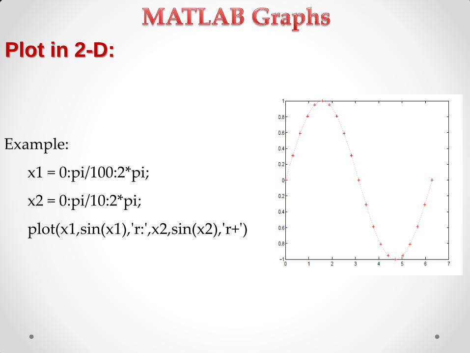
Example:
x1 = 0:pi/100:2*pi;
x2 = 0:pi/10:2*pi;
plot(x1,sin(x1),'r:',x2,sin(x2),'r+')

Plot in 2-D:
• All Properties Of Plot Command :
plot(x,y,'--rs',<
'LineWidth',2,...
'MarkerEdgeColor','k',...
'MarkerFaceColor','g',...
'MarkerSize',10)

Plot in 2-D:
• Imaginary and Complex Data:
t = 0:pi/10:2*pi;
Z=exp(i*t);
plot(real(z),imag(z))
OR
plot(z)

Exercise:
Plot the vector y with respect the vector x in
the XY plan considering style:
o Dotted line
o diamond marker
o green color
o line width of 3

Plot in 2-D:
• Adding Plots to an Existing Graph:
x1 = 0:pi/100:2*pi;
x2 = 0:pi/10:2*pi;
plot(x1,sin(x1),'r:‘)
hold on
plot(x2,sin(x2),'r+')
hold off

Plot in 2-D: • Figure Windows
o figure
o figure(n)
where n is the number in the figure title bar.
• Multiple Plots in One Figure:
x = linspace(0,2*pi,100);
y = sin(x);
y1 = cos(x);
subplot 211
plot(x, y);
subplot 212
plot(x, y1);
• area(x, y); %% think what happened ??!!!
0 1 2 3 4 5 6 7-1
-0.5
0
0.5
1
0 1 2 3 4 5 6 7-1
-0.5
0
0.5
1

Plot on 3D:
t = 0:0.1:2*pi;
x = sin(t);
y = cos(t);
plot3(x,y,t)
-1-0.8
-0.6-0.4
-0.20
0.20.4
0.60.8
1
-1
-0.5
0
0.5
1
0
1
2
3
4
5
6
7

Plot surface in the 3D :
x = linspace(1,10,20);
y = linspace(1,5,10);
[XX,YY] = meshgrid(x,y);
ZZ = sin(XX)./exp(YY);
mesh(ZZ)
02
46
810
1214
1618
20
0
2
4
6
8
10
-0.4
-0.3
-0.2
-0.1
0
0.1
0.2
0.3
0.4

Specialized Plotting Functions:
polar : to make polar plots
»polar(0:0.01:2*pi,cos((0:0.01:2*pi)*2))
•bar : to make bar graphs
»bar(1:10,rand(1,10));
•stairs : plot piecewise constant functions
»stairs(1:10,rand(1,10));
•fill : draws and fills a polygon with specified vertices
»fill([0 1 0.5],[0 0 1],'r');

Axes Control:
• For tow-dimensional graphs:
>>axis([xmin xmax ymin ymax])
• For three-dimensional graphs:
>>axis([xmin xmax ymin ymax zmin zmax])
• To reenable MATLAB automatic limit selection:
>>axis auto
• makes the x-axis and y-axis the same length:
>>axis square

Axes Control:
• Makes the axes visible (This is the default):
>>axis on
• Makes the axes invisible:
>>axis off
• Turns the grid lines on:
>>grid on
• Turns them back off again:
>>grid off

Exercise:
Plot the vector y with respect the vector x in
the XY plan considering style:
o Dotted line
o diamond marker
o green color
o line width of 3

Relational Operators:
•MATLAB uses mostlystandard relational operators
equal ==
notequal ~=
greater than >
less than <
greater or equal >=
less or equal <=
•Logical operatorselementwiseshort-circuit (scalars)
And &&
Or ||
Not~
Xor xor
•Boolean values: zero is false, nonzero is true

Relational Operators:
•MATLAB uses mostlystandard relational operators
equal ==
notequal ~=
greater than >
less than <
greater or equal >=
less or equal <=
•Logical operatorselementwiseshort-circuit (scalars)
And &&&
Or |||
Not~
Xor xor
•Boolean values: zero is false, nonzero is true

If / else / elseif :
• Basic flow-control, common to all languages
• MATLAB syntax is somewhat unique
• No need for parentheses : command blocks are between reserved
words

If / else / elseif :
a= input( ‘A‘ )
if rem(a,2) ==0
msgbox(‘a is even’);
end

If / else / elseif :
a= input( ‘A’ )
if rem(a,2) ==0
msgbox(‘a is even’);
else
msgbox(‘a is odd’);
end

If / else / elseif :
if y < 0
M = y + 3;
elseif y > 5
M = y – 3;
else
M = 0;
End
M

Switch case:
A='bye';
switch A
case 'hi'
msgbox('he says hi')
case 'bye'
msgbox('he says bye')
otherwise
msgbox('nothing')
end
Switch case:
• SWITCH expression must be a scalar or string constant.
• Unlike the C language switch statement, MATLAB switch does not
fall through.
If the first case statement is case statements do not execute.
• So, break statements are not required.

For Loop :
• For loops : use for a known number of iterations
• MATLAB syntax:
• The loop variable:
o Is defined as a vector
o Is a scalar within the command block
o Does not have to have consecutive values (but it's usually cleaner
if they're consecutive)
• The command block:
o Anything between the for line and the end

For Loop :
for n = 1:32
r(n) = n;
end
r
• Nested For Loop
for m = 1: 5
for n = 1: 7
A(m,n) = 1/(m+n-1);
end
end

While loop:
• The while is like a more general for loop:
• Don't need to know number of iterations
• The command block will execute while the conditional expression is
true
o Beware of infinite loops!

While loop:
x = 1;
while (x^2<10)
y=x^2;
plot(x,y,’or’); hold on
x = x+1;
end

Continue:
• The continue statement passes control to the next iteration of the loop
• Skipping any remaining statements in the body of the loop.
• In nested loops, continue passes control to the next iteration of the
loop enclosing it.
x=1;
for m=1:5
if (m==3)
continue;
end
x=m+x;
end
x

Continue:
• The continue statement passes control to the next iteration of the loop
• Skipping any remaining statements in the body of the loop.
• In nested loops, continue passes control to the next iteration of the
loop enclosing it.
• Example: x=1;
for m=1:5
if (m==3)
continue;
end
x=m+x;
end
x

Break:
• The break statement lets you exit early from a for loop or while loop.
• In nested loops, break exits from the innermost loop only.
• Example:
x=1;
for m=1:5
if (m==3)
break;
end
x=m+x;
end
x

Error Trapping:
A= input( ‘ Matrix = ‘ )
try
B = inv (A);
catch
msgbox(‘Matrix is not square’)
end

User-defined Functions:
Functions look exactly like scripts, but for ONE difference
Functions must have a function declaration.
No need for return :
MATLAB 'returns' the variables whose names match those in the
function declaration.

User-defined Functions:

User-defined Functions:
MATLAB provides three basic types of variables: Local Variables:
Each MATLAB function has its own local variables. Global Variables:
If several functions, and possibly the base workspace, all declare a particular name as global, then they all share a single copy of that variable.
Persistent Variables: You can declare and use them within M-file functions only. Only the function in which the variables are declared is allowed access to it.

User-defined Functions:
%this fun. To sum 2 no’s.
function x=SUM2(a,b)
global z
x=a+b+z;
end
%this fun. To sum 2 no’s.
function x=SUM2(a,b)
x=a+b;
end
Matrix :
1-One dimension matrix
Only one row or one column (vector)
2-Two dimensions
Has rows and columns
3-three dimension matrix (multidimensional array)
Has rows, columns and pages.

Matrix :
Create the 3D matrix
>> M=ones(4,4,4)

Matrix :

Cell Array:
• Used to store different data type (classes) like vectors, matrices,
strings,<etc in single variable.
• Variables declaration: >> X=3 >> Y=[1 2 3;4 5 6] >> Z(2,5)=15 >> A(4,6)=[3 4 5] %…..(wrong)
• cell array: >> C{1}=[2 3 5 10 20] >> C{2}=‘hello’ >> C{3}=eye(3)
1 0 0
0 1 0
0 0 1
C
2 3 5 10 20 h e l l o

Cell Array:
Z{2,5} = linspace(0,1,10) Z{1,3} = randint(5,5,[0 100]) Z{1,3}(4,2) =77 Note: • The default for cell array elements is empty • The default for matrix elements is zero
77
Z

Structure Array:
• Variables with named ‚data container‛ called fields.
• The field can contain any kind of data.
• Example:
>> Student.name=‘Ali’;
>> Student.age=20;
>> Student.grade=‘Excellent’;
Student
age name grade

Structure Array:
>> manager = struct ('Name', 'Ahmed', 'ID', 10, 'Salary', 1000)
manager =
Name: 'Ahmed'
ID: 10
Salary: 1000

Structure Array:
>> manager(3)=struct ('Name', 'Ali','ID',20, 'Salary',2000)
manager =
1x3 struct array with fields:
Name
ID
Salary

Structure Array:
• The need of Structure Array
x.y.z = 3
x.y.w = [ 1 2 3]
x.p = ‘hello’
• Note: x can be array
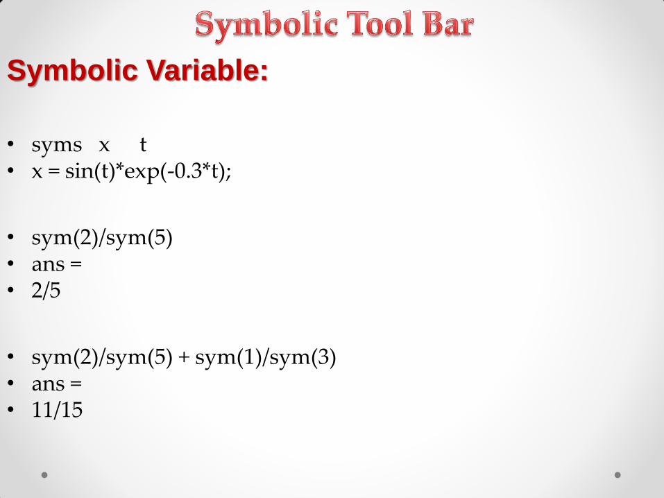
Symbolic Variable:
• syms x t • x = sin(t)*exp(-0.3*t);
• sym(2)/sym(5) • ans = • 2/5
• sym(2)/sym(5) + sym(1)/sym(3) • ans = • 11/15
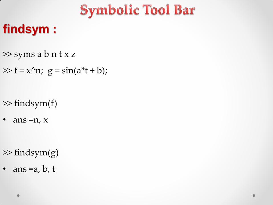
findsym :
>> syms a b n t x z
>> f = x^n; g = sin(a*t + b);
>> findsym(f)
• ans =n, x
>> findsym(g)
• ans =a, b, t

subs :
>> f = 2*x^2 - 3*x + 1 >> subs(f,2) ans =3
>> syms x y
>> f = x^2*y + 5*x*sqrt(y)
>> subs(f, x, 3)
ans = 9*y+15*y^(1/2)
>> subs(f, y, 3)
ans = 3*x^2+5*x*3^(1/2)
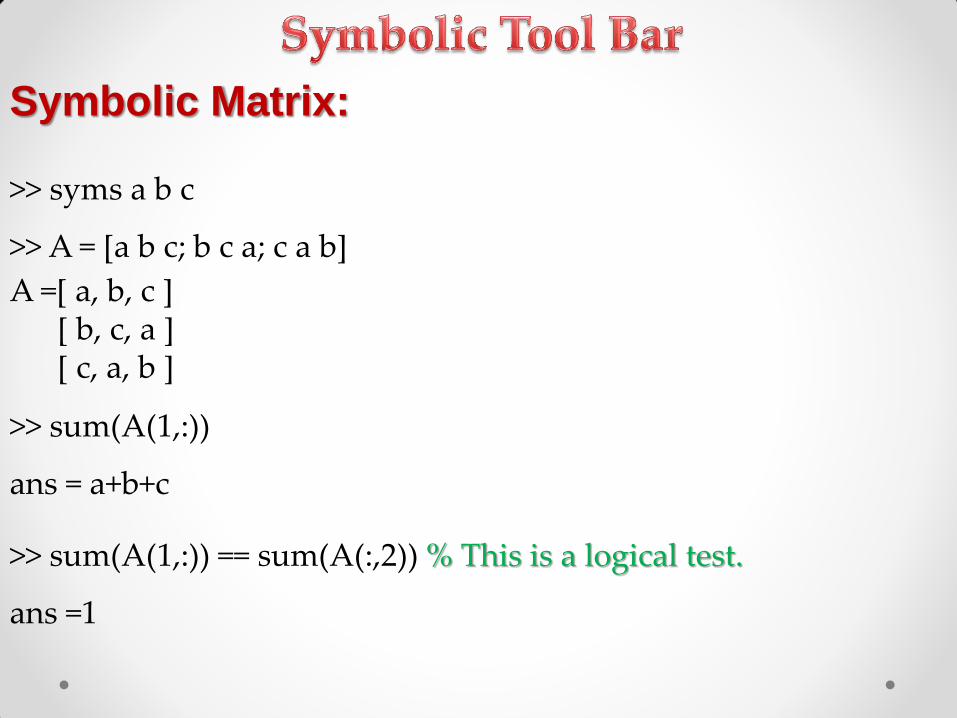
Symbolic Matrix:
>> syms a b c
>> A = [a b c; b c a; c a b]
A =[ a, b, c ] [ b, c, a ] [ c, a, b ]
>> sum(A(1,:))
ans = a+b+c
>> sum(A(1,:)) == sum(A(:,2)) % This is a logical test.
ans =1

Simple:
• Simplify the expression.
>> syms x
>> m = sin(x)/cos(x)
>> simple(m)
• Show expression in a user friendly format
>> m = sin(x)/cos(x)
>> pretty(m)
Pretty:
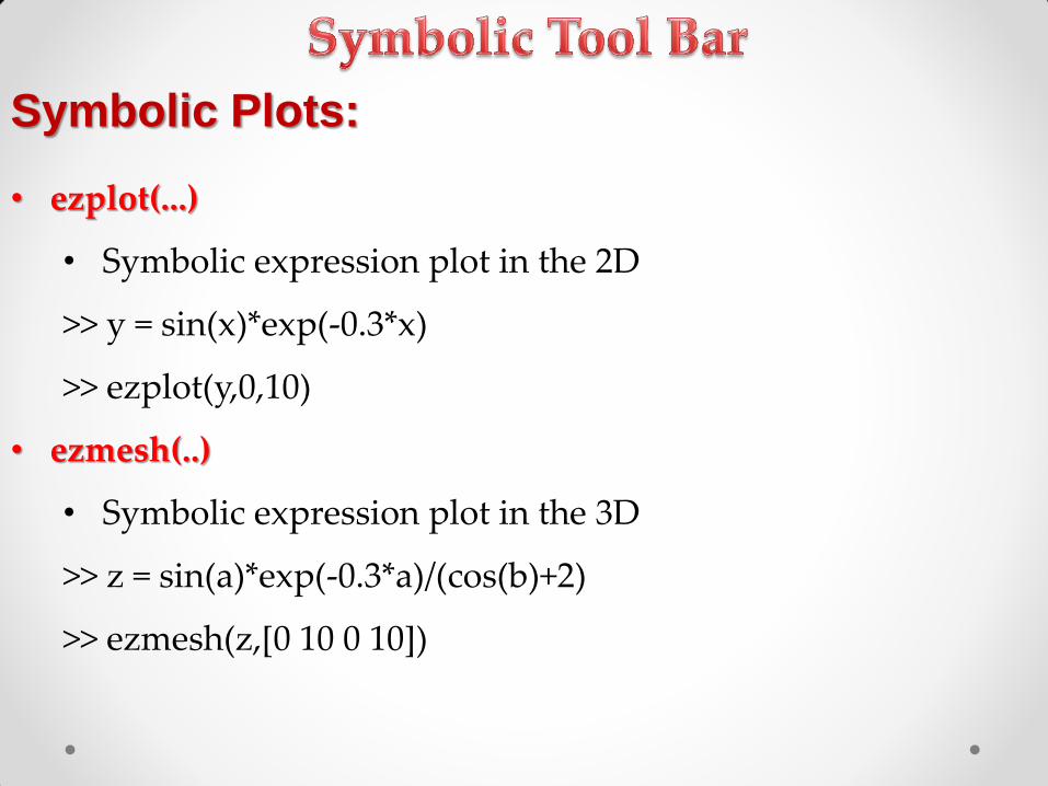
Symbolic Plots:
• ezplot(...)
• Symbolic expression plot in the 2D
>> y = sin(x)*exp(-0.3*x)
>> ezplot(y,0,10)
• ezmesh(..)
• Symbolic expression plot in the 3D
>> z = sin(a)*exp(-0.3*a)/(cos(b)+2)
>> ezmesh(z,[0 10 0 10])

Limit:
>> syms h n x
>> limit( (cos(x+h) - cos(x))/h,h,0 )

Differentiation diff :
• Numerical Difference or Symbolic Differentiation
>> z = [1, 3, 5, 7, 9, 11];
>> dz = diff(z)
>> Syms x t
>> x=t^4;
>> xd3 = diff(x,3)

Differentiation diff(…) :
>> syms s t
>> f = sin(s*t)
>> diff(f,t)
ans = cos(s*t)*s
>> diff(f,t,2)
ans =-sin(s*t)*s^2
>> diff(y)./diff(x)

Integration int(…)
• Symbolic integration
>> int(y)
• Integration from 0 to 1
>> int(x,0,1)
• Integration from 0 to 2
>> int(x,0,2)

solve equation solve(...):
>> syms x y real
>> eq1 = x+y-5
>> eq2 = x*y-6
>> [xa, ya] = solve(eq1, eq2)
OR
>> answer = solve(eq1, eq2)
answer.x
answer.y
>> syms x y real
>> s = solve('x+y=9','x*y=20')

Differential Equations dsolve(..):
• Symbolic solution of ordinary differential equations
>> syms x real
>> diff_eq_sol = dsolve('m*D2x+b*Dx+k*x=0','Dx(0)=-1','x(0)=2')
>> syms m b k real
>> subs(diff_eq_sol, [m,b,k], [2,5,100])