matlab programming i joy. outline examples what is matlab? history characteristics organization of...
TRANSCRIPT

MATLAB Programming I
Joy

Outline
• Examples
• What is Matlab?
• History
• Characteristics
• Organization of Matlab – Toolboxes
• Basic Applications
• Programming

Example I
• Obtain the result of matrix multiply
• Matlab Code >>A=[4,6; 9,15; 8,7]; >>B=[3,24,5; 7,19,2]; >>C=A*B C = 54 210 32 132 501 75 73 325 54
4 63 24 5
9 157 19 2
8 7

C Code
#include <cstdlib>#include <iostream>#include <fstream>#include <sstream>#include <iomanip>#include <vector>
using namespace std;typedef vector<vector<int> > Mat;void input(istream& in, Mat& a);Mat matrix_product(const Mat& a, const Mat& b);void print(const Mat& a);
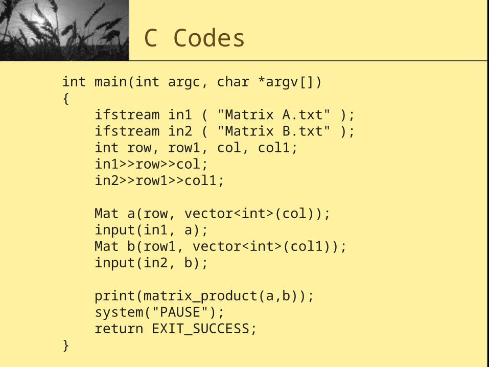
C Codes
int main(int argc, char *argv[]){ ifstream in1 ( "Matrix A.txt" ); ifstream in2 ( "Matrix B.txt" ); int row, row1, col, col1; in1>>row>>col; in2>>row1>>col1;
Mat a(row, vector<int>(col)); input(in1, a); Mat b(row1, vector<int>(col1)); input(in2, b); print(matrix_product(a,b)); system("PAUSE"); return EXIT_SUCCESS;}

C Code Cond.void input(istream& in, Mat& a){ for(int i = 0; i < a.size(); ++i) for(int j = 0; j < a[0].size(); ++j) in>>a[i][j];}
void print(const Mat& a){ for(int i = 0; i < a.size(); ++i) { cout<<endl; for(int j = 0; j < a[0].size(); ++j) cout<<setw(5)<<a[i][j]; } cout<<endl; }

C Code Cond.
Mat matrix_product(const Mat& a, const Mat& b){ Mat c(a.size(), vector<int>(b[0].size())); for(int i = 0; i < c.size(); ++i) for(int j = 0; j < c[0].size(); ++j) { c[i][j] = 0; for(int k = 0; k < b.size() ; ++k) c[i][j] = c[i][j] + a[i][k] * b[k][j]; } return c;}

Example II
• Calculate the transpose of the matrix:
• Matlab Code >>A=[3,17,2;5,19,7;6,4,54] >>A^(-1)
ans = -0.9327 0.8505 -0.0757 0.2131 -0.1402 0.0103 0.0879 -0.0841 0.0262
3 17 2
5 19 7
6 4 54

What is MATLAB?
• Abbreviation of MATrix LABoratory
• Is a high-performance language for technical computing
• It integrates computation, visualization, and programming in an easy-to-use environment where problems and solutions are expressed in familiar mathematical notation.

Usage of MATLAB
• Math and computation • Algorithm development • Data acquisition • Modeling, simulation, and prototyping • Data analysis, exploration, and visualization • Scientific and engineering graphics • Application development
including graphical user interface building

History
• In 1970s – Dr.Cleve Moler Based on Fortran on EISPACK and LINPACK Only solve basic matrix calculation and graphic• 1984 – MathWorks Company by Cleve Moler and
Jack Little Matlab 1.0 based on C Included image manipulations, multimedia etc.
toolboxes• In 1990 – run on Windows Simulink, Notebook, Symbol Operation, etc.• 21 Century
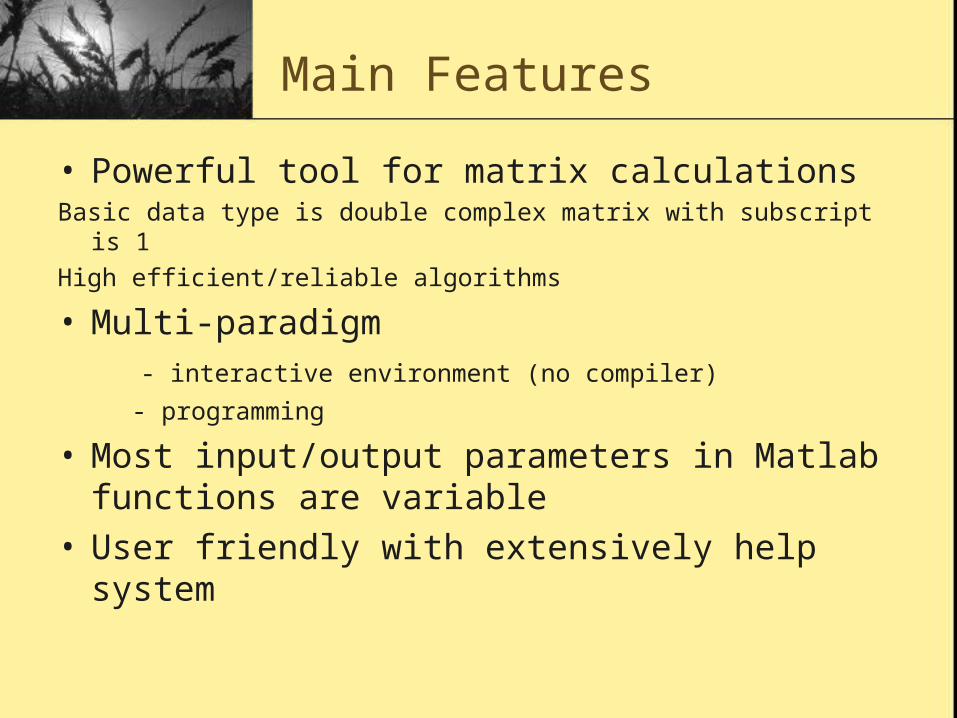
Main Features
• Powerful tool for matrix calculationsBasic data type is double complex matrix with subscript is 1
High efficient/reliable algorithms
• Multi-paradigm - interactive environment (no compiler)
- programming
• Most input/output parameters in Matlab functions are variable
• User friendly with extensively help system

MATLAB SYSTEM
Develop Tools
Toolboxes
Data-Accessing Tools
Stateflow
Generating-Codes Tools
Module Libraries
Third parties modules
Applications
DATA
C
Simulink
MATLAB

Buildup of MATLAB
• Development Environment MATLAB desktop and Command Window, a command history, an editor
and debugger, and browsers for viewing help, the workspace, files, and the search path.
• The MATLAB Mathematical Function Library A vast collection of computational algorithms ranging from elementary
functions to more sophisticated functions
• The MATLAB Language A high-level matrix/array language with control flow statements,
functions, data structures, input/output, and object-oriented programming features
• Graphics Display vectors and matrices as graphs two-dimensional and three-dimensional data visualization image processing animation and presentation graphics
• The MATLAB Application Program Interface (API) Interchange the C/Fortran codes with Matlab codes

Basic Applications I
• Matrices and Arrays Generating Arrays/Matrices Elementary Matrices: sum, transpose, diagonal, subscripts Variables: does not require any type
declarations or dimension statements Operators: +,-,*,/, ^, etc. Examples of Expressions

Generating Matrices
• Directly enter
A = [16 3 2 13; 5 10 11 8; 9 6 7 12; 4 15 14 1]
• Use Functions
Example: B = zeros(1,5) – row vector/array
C = ones(7,1) –column vector/array
D = rand(5,8,3) – multiple dimension matrix
• Load/Import from files
zeros All 0’s
ones All 1’s
rand Uniformly distributed random elements
randn Normally distributed random elements

Elementary Matrices>>D=rand(3,2,3)D(:,:,1) = D(:,:,2) = D(:,:,3) = 0.9501 0.4860 0.4565 0.4447 0.9218 0.4057 0.2311 0.8913 0.0185 0.6154 0.7382 0.9355 0.6068 0.7621 0.8214 0.7919 0.1763 0.9169>> sum(D(:,1,1))ans = 1.7881>> E=D(:,:,2)'E = 0.4565 0.0185 0.8214 0.4447 0.6154 0.7919>> a=diag(D(:,:,3))a = 0.9218 0.9355>> F=[D(1,:,1),D(2,:,3); D(1,:,1)+1, D(2,:,3)-1]F = 0.9501 0.4860 0.7382 0.9355 1.9501 1.4860 -0.2618 -0.0645>>F(:,2)=[]F = 0.9501 0.7382 0.9355 1.9501 -0.2618 -0.0645>> F(2:1:4)=[]F = 0.9501 0.9355 -0.0645

Examples of Expression
>>rho = (1+sqrt(5))/2rho = 1.6180
>>a = abs(3+4i)a = 5
>>huge = exp(log(realmax))huge = 1.7977e+308 =1.8X10308

Basic Application II
• Graphic

Programming
• Flow Control
Selector: if, switch & case
Loop: for, while, continue, break, try & catch
Other: return• Other Data Structures
Multidimensional arrays, Cell arrays, Structures, etc.
• Scripts and Functions

Flow Control Examples I
• Selector:2-way:if rand < 0.3 %Condition flag = 0; %then_expression_1else flag = 1; %then_expression_2end %endif Multiple-ways:
if A > B | switch (grade) 'greater‘ | case 0elseif A < B | ‘Excellent’ 'less‘ | case 1elseif A == B | ‘Good’ 'equal‘ | case 2else | ‘Average’ error('Unexpected situation') | otherwiseend | ‘Failed’ | end

Flow Control Examples II
• Loop>>Generate a matrix
for i = 1:2
for j = 1:6
H(i,j) = 1/(i+j);
end
end
>>HH =
0.5000 0.3333 0.2500 0.2000 0.1667 0.1429
0.3333 0.2500 0.2000 0.1667 0.1429 0.1250

• Loop Cond.>>%Obtain the result is a root of the polynomial x3 - 2x – 5a = 0; fa = -Inf; b = 3; fb = Inf;while b-a > eps*b x = (a+b)/2; fx = x^3-2*x-5; if sign(fx) == sign(fa) a = x; fa = fx; else b = x; fb = fx; endend>>x
x = 2.09455148154233

Scripts
• MATLAB simply executes the commands found in the file
• Example % Investigate the rank of magic squares r = zeros(1,32); %generation a row array 1X 32 % “;” tell the system does not display % the result on the screen for n = 3:32 r(n) = rank(magic(n)); end r bar(r) %display r in bar figure

Scripts Cond.
• Note:
No input/output parameters
(Different from functions! )
Write the script in editor, which can be
activated by command “edit” in command
window, save it with its specific name
Next time you want to execute the script just
call the name in the command window
Functions
• Functions are M-files that can accept input arguments and return output arguments. The names of the M-file and of the function should be the same.

Function Example I
• Background of AIC
AIC is used to compare the quality of nested models
AIC requires a bias-adjustment in small sample sizes
1
2 ln( ) 2
2 ( 1)2 ln( ) 2
1min( )
exp( 0.5 )
exp( 0.5 )
i i
ii R
rr
AIC likelihood K
K KAICad likelihood K
n Kdelta AIC AIC
deltaw
delta

Function Head (Comments)
%AICad Function%Date:Dec.29th, 2008 %Purpose: Calculate the adjusted % Akaike’s Information Criteria (AIC)%InPut: AIC % n (the sample size)% K (the number of parameters in the model)%OutPut: AICad% delta% weight%Functions Called: None%Called by: None

IN Command Window
>>AIC=[-123; -241.7; -92.4; -256.9]; >>n=12;>>K=[4;8;2;6];>>[AICad, delta, w] = CalAIC(AIC, n, K)AICad = delta = w =
-83.0000 89.9000 0.0000 -97.7000 75.2000 0.0000 -80.4000 92.5000 0.0000 -172.9000 0 1.0000

M file
function[AICad,delta,w]=CalAIC(AIC,n,K)
AICad = AIC+2.*K.*(K+1);
a = min(AICad);
delta = AICad - a;
b = exp(-0.5.*delta);
c = sum(b);
w = b./c;

Function Example II
• Background of PCA
Comparing more than two communities or samples
Sample Post Oak Red Oak Water Oak
1 66 25 24
2 48 30 31
3 26 55 42
4 15 20 49
5 11 50 58
combine post post red red water waterY w x w x w x
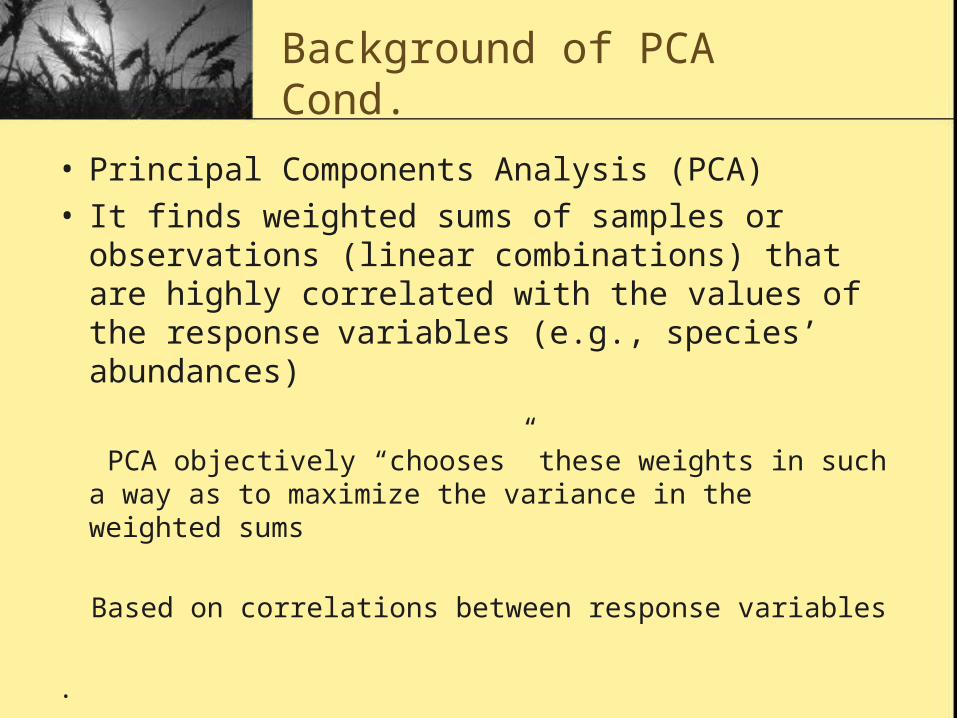
Background of PCA Cond.
• Principal Components Analysis (PCA) • It finds weighted sums of samples or
observations (linear combinations) that are highly correlated with the values of the response
variables (e.g., species’ abundances)
PCA objectively “chooses” these weights in such a way as to maximize the variance in the weighted sums
Based on correlations between response variables
.

Function Head
%Principle Component Analysis Function%Date:Dec.29th, 2008 %Purpose: Obtain the axis scores of PCA%InPut: the abundance of 3 species % in 5 different samples %OutPut: sample scores of PCA axis%Functions Called: None%Called by: None

IN Command Window
>>a=[66;48;26;15;11];>>b=[25;30;55;20;50];>>c=[24;31;42;49;58];>>[score1, score2]=PCA(a,b,c)score1 = score2 = -2.2233 -0.1963 -1.1519 -0.0743 0.8734 -1.0888 0.4871 1.5120 2.0147 -0.1526

M file
function[x11,x12,x13,x21,x22,x23]=PCA(a,b,c)
%Calculate the mean and population standard deviation of 3 speciesfor i=1:5 d(i)=(a(i)-mean(a))^2; stda=sqrt(sum(d)/5); e(i)=(b(i)-mean(b))^2; stdb=sqrt(sum(e)/5); f(i)=(c(i)-mean(c))^2; stdc=sqrt(sum(f)/5);end%Obtain the z-scores of 3 speciesfor i=1:5 za(i)=(a(i)-mean(a))/stda; zb(i)=(b(i)-mean(b))/stdb; zc(i)=(c(i)-mean(c))/stdc;endN=[za',zb',zc'];

M file Cond.
%Obtain the original correlation matrixM=[1,corr(a,b),corr(a,c);corr(a,b),1,corr(b,c);corr(a,c),corr(b,c),1];[V1,D1]= eig(M); %Calculate the eigenvector and eigenvaluesweight1=V1(:,3); %Get the maximum eigenvectorscore1=N*weight1;
%We use the exact same procedure that we used for axis 1, %except that we use a partial correlation matrix %The partial correlation matrix is made up of all pairwise correlations%among the 3 species, independent of their correlation with the axis 1%sample scores. Hence, axis 2 sample scores will be uncorrelated %with (or orthogonal to) axis 1 scores.

M file Cond.
new=[a,b,c,score1];M2=[1,corr(a,b),corr(a,c),corr(a,score1);… corr(a,b),1,corr(b,c),corr(b,score1);… corr(a,c), corr(b, c), 1, corr(c,score1);… corr(a,score1),corr(b,score1),corr(c,score1),1];for i=1:3 for j=1:3 corrnew(i,j)=M2(i,j); endendg=[M2(4,1)*M2(4,1),M2(4,1)*M2(4,2),M2(4,1)*M2(4,3);… M2(4,2)*M2(4,1),M2(4,2)*M2(4,2),M2(4,2)*M2(4,3);… M2(4,3)*M2(4,1),M2(4,3)*M2(4,2),M2(4,3)*M2(4,3)];corrmatrix=corrnew-g;[V2,D2]=eig(corrmatrix);weight2=V2(:,3); %signs needs to be checked with JMPscore2=N*weight2;

MATLAB in MCSR
• Matlab is available on willow and sweetgum
• www.mcsr.olemiss.edu


• Enter matlab can activate Matlab in willow or sweetgum
• Use ver to obtain the version of Matlab, which can tell you which toolboxes of Matlab in that machine
• Price of personal purchase is 500$ include update releases (only include MATLAB & Simulink)
You need pay separate fee for each toolbox such as statistical, bioinformatics, etc

Take Home Message
