mbd week 4 2017 - lth · 19 the configuration space: s2 o ... the planar double pendulum has two...
TRANSCRIPT

2017-02-15
1
The MultiBody
1
Examination task 2: Problem 2:3
Weld (between cone and axle BC)
2
The Multibody
Revolute Joint
3
Vehicle driveline
The Multibody
4
The Multibody
...
5
1
...
3
4
2
, ,..., ,1 N
N
1
,
Part
Joint
5
Degrees of freedom and coordinates
( )Oi j k
( , , ) R Rc O c c cx x i j kx y z
( ) ( ), c cx X x X X X R 0B
, , ,c c c x y z
fixed in frame
Rigid transplacement:
, , Configuration coordinates:
Configuration manifold: ( )SOE V
(6 DOF, Gross)
6
2017-02-15
2
Degrees of freedom and coordinates
, , ... , , 1 2 6 N 1 6 N
Multibody containing N rigid parts: , ,...,1 N
Configuration coordinates:
, , , , , , ... , etc.1 1 2 1 3 1 4 1 5 1 6 1c c c x y z
Configuration
(6N DOF, Gross)
7
Degrees of freedom and coordinates
( ), .t t 0 T
( ( )) ( ( ))( ), c cx t t X X X R 0B
Motion:
( , ) ( ( ); )x X t t X
8
1
2
6 N
( )t
Constraints
, ,...,6 N
ki ii k
k 1
0 i 1 mt
C CC
( , ) ( , , , ... , , )
( , ) ( , , , ... , , )
( , ) ( , , , ... , , )
1 2 6 N 1 6 N
1 2 6 N 1 6 N
1 2 6 N 1 6 N
t t 0
t t 0
t t 0
1 1
2 2
m m
C C
C C
C C
Number of constraint equations: m
( )( ) ,m 6 Nij
C Constraint matrix: ( )i
jrank m
C
Holonomic kinematical constraints:
Geometrical constraints:
9
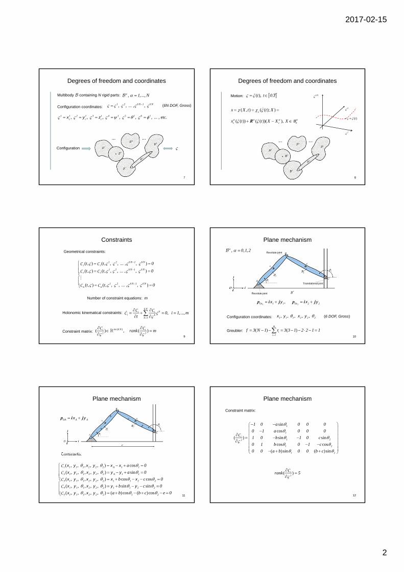
Plane mechanism
,1Oc 1 1 p i jx y
2Oc 2 2 p i jx y
, , ,1 1 1x yConfiguration coordinates: (6 DOF, Gross), , 2 2 2x y
, , ,0 1 2
Greubler: ( ) ( )m
ii 1
f 3 N 1 r 3 3 1 2 2 1 1
Revolute joint
Revolute joint
Translational joint
0
10
Plane mechanism
( , , , , , ) cos
( , , , , , ) sin
( , , , , , ) cos cos
( , , , , , ) sin sin
( , , , , , )
1 1 1 2 2 2 A 1 1
2 1 1 1 2 2 2 A 1 1
3 1 1 1 2 2 2 1 1 2 2
4 1 1 1 2 2 2 1 1 2 2
5 1 1 1 2 2 2
a 0
a 0
b c 0
b c 0
1C
C
C
C
C
x y x y x x
x y x y y y
x y x y x x
x y x y y y
x y x y ( ) cos ( ) cos1 2a b b c e 0
Constraints:
OA A A p i jx y
11
Plane mechanism
sin
cos
( ) sin sin
cos cos
( )sin ( )sin
1
1
i1 2j
1 2
1 2
1 0 a 0 0 0
0 1 a 0 0 0
1 0 b 1 0 c
0 1 b 0 1 c
0 0 a b 0 0 b c
C
Constraint matrix:
( )ij
rank 5
C
12
2017-02-15
3
Configuration space (manifold)
( ) ( , ) , ,...,6 Nt i t 0 i 1 m CC
, , ... , 1 2 nq q q q
ˆ( ) ( , ), nt t q q C
( , ) ( , ( ), ( ),..., ( ); ) ( , ( ); )1 2 nq qx X t t q t q t q t X t q t X
( )q q t
Configuration coordinates:
n 6 N m
Motion:
ˆ( , ) t q
n-dimensional surface in 6 N
13
Multibody in motion
0B
X
tB
x
1q
( )q q t
- : nq space
nq
( , ; )q t q
( , ; ) ( , ) ( , )( ), , ( )q c ct q X x t q t q X X X q q t R 0B
Rigid body:
14
Rheonomic and scleronomic coordinate systems
( , ) ( , ( ), ( ),..., ( ); ) ( , ( ); )1 2 nq qx X t t q t q t q t X t q t X
( , ) ( ( ), ( ),..., ( ); ) ( ( ); )1 2 nq qx X t q t q t q t X q t X
Scleronomic, no explicit time dependence:
Rheonomic, explicit time dependence:
Partial derivatives: ( , , ,..., ; ) ( , ; )1 2 nq qx t q q q X t q X
, ,..., ,q q q q
1 nt q q X
15
, , , nt 0 T q X 0B x
y
r
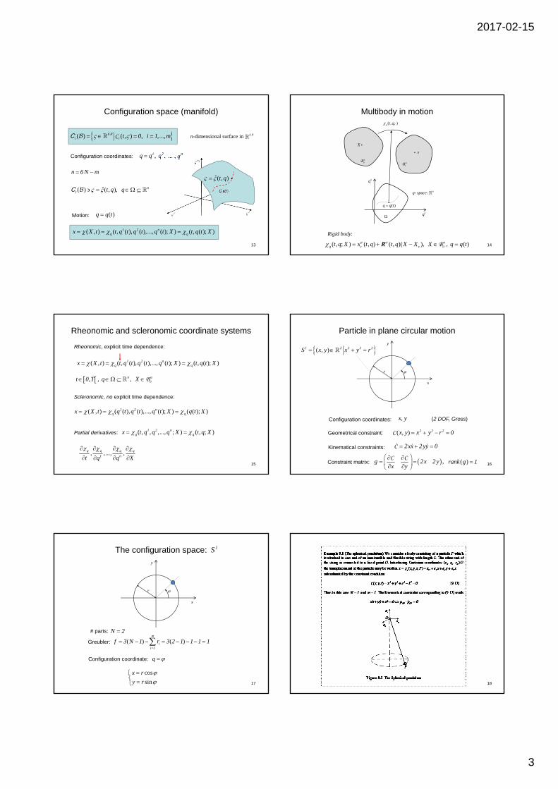
Particle in plane circular motion
Geometrical constraint: ( , ) 2 2 2x y x y r 0 C
Kinematical constraints: 2xx 2 yy 0 C
Constraint matrix: ,g 2x 2 yx y
C C
( , )1 2 2 2 2S x y x y r
( )rank g 1 16
Configuration coordinates: ,x y (2 DOF, Gross)
The configuration space:
x
y
r
Configuration coordinate: q
Greubler: ( ) ( )m
ii 1
f 3 N 1 r 3 2 1 1 1 1
cos
sin
x r
y r
N 2# parts:
17
1S
18

2017-02-15
4
Example 9.1 continued. We have
2
C C CC = x y z
x y z
and then ( ) , if ( ) ( )rank 1 0 0 0 x,y,z , ,C . Since n 3N m 3 1 2 , the configuration space of the particle
( ) ( ) ( )3P 0 x,y,z x,y,zCC
is a 2-dimensional surface in 3 , the sphere 2S . As configuration coordinates one may use angles ( , ) belonging to the spherical coordinate system. Then
sin cos
sin sin
cos
L
L
L
x
y
z
19
The configuration space: 2S
O
c
1
0
i
j
k
The planar pendulum
, , c c x yConfiguration coordinates:
( ) ( )m
ii 1
f 3 N 1 r 3 2 1 2 1
Revolute joint
N 2# parts:
20
(3 DOF, Gross)
( , , ) sin,
( , , ) cos
c c c O
2 c c c O
l0
2l
02
x y x x
x y y y
1C
CConstraints: m 2
cos,
sin
1 1 1
c c
2 2 2
c c
C C C l1 0
2gC C C l
0 12
x y
x y
Constraint matrix:
( )rank g 2
21
1SThe configuration space: Example 9.2 (The planar double pendulum). The planar double pendulum consists of two homogeneous, rigid and slender bars 1 and 2 of the same material with masses 1m and
2m , lengths 1l and 2l , respectively. The bars are connected by an ideal revolute joint at
point A and 1 is connected to the roof 0 by an ideal revolute joint at point O. See the figure below. The pendulum may move in a vertical plane. Figure 9.6 The planar double pendulum.
i
j
k
g 0
A
B
1
2
O
22( ) ( )
m
ii 1
f 3 N 1 r 3 3 1 2 2 2
Example 9.2 continued. The planar double pendulum has two degrees of freedom. We introduce angular configuration coordinates 1q and 2q according to the Figure 9.6. Considering the bars as one-dimensional parts, the transplacement of the double pendulum may be written
( sin cos ) , , ( )( , ; )
( sin cos ) ( sin cos ) , , ( )
1O 1
q 2O 1 2
x X 0 X l forx X
x l X 0 X l for
i j
i j i j
( , ) ( , ) , 2 where the RON-basis ( , , )i j k is shown in
the figure above. The configuration coordinate system is thus scleronomic. Note that the transplacement for 2 may be written
( , ; ) ( sin sin ) ( cos cos ), q O 1 1 2x X x l X l X 0 X l i j
The configuration space is, in this case, a torus 1 1T S S .
23
The configuration space: T Multibody kinematics
q q
k kq q
x
( , , ; )n
q q kq k
k 1
t q q X qt q
x x
( , ) ( , ( ), ( ),..., ( ); ) ( , ( ); ), 1 2 nq qx X t t q t q t q t X t q t X X 0B
1q
q
- : nq space
nq
q
Motion:
Velocity:
Generalized velocity: ( )1 nq q q
( )q q t
24
2017-02-15
5
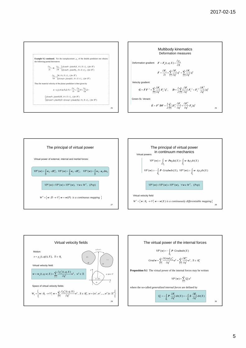
Example 9.2 continued. For the transplacement q of the double pendulum one obtains
the following partial derivatives
q
t
0 ,
( cos sin ) , , ( )
( cos sin ) , , ( )
1q 1
21 2
X 0 X l for
l 0 X l for
i j
i j
, , ( )
( cos sin ) , , ( )
1q 1
22
0 X l for
X 0 X l for
0
i j
Thus the material velocity of the planar pendulum is then given by
( , , , , ; ) q q qq t X
t
x x
( cos sin ) , , ( )
(( cos sin ) ( cos sin ) , , ( )
11
21 2
X 0 X l for
l X 0 X l for
i j
i j i j
25
,n
q1 1 kqk
k 0
F
G FF F
n nq q qk k
k kk 1 k 0
q qt q q
F F F
F
( , ; ) qq t q X
X
F F
( )Tn
q q1 T kq qk k
k 0
1q
2 q q
F F
D F F
( )Tn
q qT T kq qk k
k 0
1q
2 q q
F F
E F DF F F
Multibody kinematicsDeformation measures
Deformation gradient:
Velocity gradient:
Green-St. Venant:
26
The principal of virtual power
( ) ( ) ( ), , ( )e i a 0VP VP VP W Pvp w w w w
( ) ,e eP PVP d w w F
( ) ,i iP PVP d w w F
( )aP P PVP dm w w a
Virtual power of external, internal and inertial forces:
27
: ( ) 0W P is a continuous mapping w w wV
The principal of virtual powerin continuum mechanics
: ( ) 1W X is a continuously differentiable mapping w w w0B V
( ) : ( ) ( )e0 0VP da X dv X
w w Pn w b
00PP
( ) : ( ),iVP Grad dv X w P w0B
( ) : ( )a0VP dv X w w x
0P
Virtual powers:
Virtual velocity field:
28
( ) ( ) ( ), , ( )e i a 0VP VP VP W Pvp w w w w
Virtual velocity fields
( , ( ); ), qx t q t X X 0B
( , ; )( , , ; ) ,
nq k k
q kk 1
t q Xt q w X w w
q
w w
( , ; ): , , ( , ,..., )
nq k 1 2 n n
q 0kk 1
t q XW w X w w w w
q
w w0B V B
0B
X
tB
x
1q
( )q q t
- : nq space
nq
( , ; )q t q
Motion:
Virtual velocity field:
Space of virtual velocity fields:
29
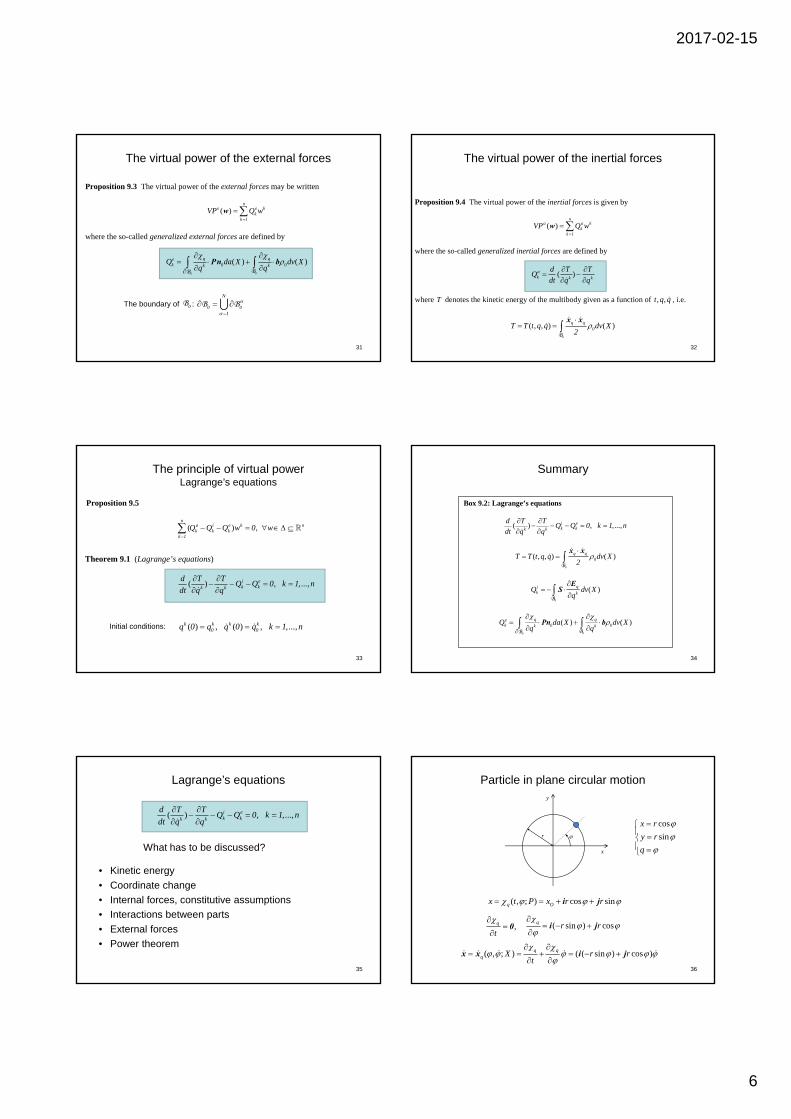
The virtual power of the internal forces
, n n
q qk k0k k
k 1 k 1
GradGrad w w X
q q
F
w B
( ) ( )iVP Grad dv X w P w0B
Proposition 9.1 The virtual power of the internal forces may be written
( )n
i i kk
k 1
VP Q w
w
where the so-called generalized internal forces are defined by
( ) ( )q qik k k
Q dv X dv Xq q
F E
P S0 0B B
30
2017-02-15
6
The virtual power of the external forces
Proposition 9.3 The virtual power of the external forces may be written
( )n
e e kk
k 1
VP Q w
w
where the so-called generalized external forces are defined by
( ) ( )q qek 0 0k k
Q da X dv Xq q
Pn b00 BB
N
1
0 0B BThe boundary of :0B
31
The virtual power of the inertial forces
Proposition 9.4 The virtual power of the inertial forces is given by
( )n
a a kk
k 1
VP Q w
w
where the so-called generalized inertial forces are defined by
( )ak k k
d T TQ
dt q q
where T denotes the kinetic energy of the multibody given as a function of , ,t q q , i.e.
( , , ) ( )q q0T T t q q dv X
2
x x
0B
32
The principle of virtual powerLagrange’s equations
Proposition 9.5
( ) , n
a i e k nk k k
k 1
Q Q Q w 0 w
Theorem 9.1 (Lagrange’s equations)
( ) , ,...,i ek kk k
d T TQ Q 0 k 1 n
dt q q
( ) , ( ) , ,...,k k k k0 0q 0 q q 0 q k 1 n Initial conditions:
33
Box 9.2: Lagrange’s equations
( ) , ,...,i ek kk k
d T TQ Q 0 k 1 n
dt q q
( , , ) ( )q q0T T t q q dv X
2
x x
0B
( )qik k
Q dv Xq
E
S0B
( ) ( )q qek 0 0k k
Q da X dv Xq q
Pn b00 BB
Summary
34
Lagrange’s equations
What has to be discussed?
• Kinetic energy
• Coordinate change
• Internal forces, constitutive assumptions
• Interactions between parts
• External forces
• Power theorem
( ) , ,...,i ek kk k
d T TQ Q 0 k 1 n
dt q q
35
Particle in plane circular motion
x
y
r
cos
sin
x r
y r
q
36
( , ; ) cos sinq Ox t P x r r i j
,q
t
0 ( sin ) cosq r r
i j
( , ; ) ( ( sin ) cos )q qq X r r
t
x x i j

2017-02-15
7
Particle in plane circular motionKinetic energy
x
y
r
( , ) ( ( sin ) cos )2 2 2 2 2k
1 1 1E T m r r m r m
2 2 2 x i j
37
Particle in plane circular motionExternal forces, internal forces
x
y
r
( )g g j
38
mgN
O
P
( )
e
q
mg
m
0
m
j
F N g
N
g
( )q q qe eQ m m
F N g g
q
iQ 0
( ( sin ) cos ) cosr r m mgr i j g
Particle in plane circular motionLagranges equations
39
x
y
r ( , ) ,2 21
T r m2
,2Tr m
T0
( ) cos cosi e 2d T T gQ Q 0 r m mgr 0 0
dt r
cos ,eQ mgr iQ 0
Lagranges equations:
40
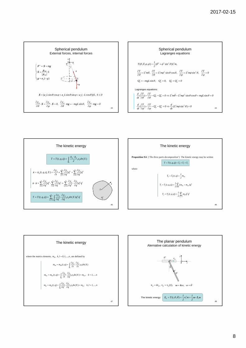
The spherical pendulum
sin cos
sin sin
cos
, 1 2
x
y
z
L
L
L
q q
( , , ; ) sin cos sin sin ( cos )q O x y zx t P x L L L e e e
,q
t
0
( sin sin ) sin cosqx yL L
e e
cos cos cos sin sin ,qx y zL L L
e e e
( )z g g e
41
The spherical pendulumMaterial velocity
L
( , , ; ) ( cos cos cos sinq q qq x yt q q X L L
t
x x e e
sin ) ( ( sin sin ) sin cos )z x yL L L e e e
( cos cos sin sin ) ( cos sin sin cos ) sinx y zL L L e e e 42
The spherical pendulumKinetic energy
( , , , ) ( sin )2 2 2 2 2k
1 1E T m L m
2 2 x
L
2017-02-15
8
43
mg
S
( )
e
OP
OP
z
m
S
g
F S g
pS
p
g e
Spherical pendulumExternal forces, internal forces
( sin cos sin sin ( cos )) , x y zL L L S S 0 S e e e
,q q 0
S S sin ,q m mgL
g q m 0
g
44
Spherical pendulumLagranges equations
( , , , ) ( sin ) ,2 2 2 21T L m
2
,2TL m
sin ,2 2T
L m
( ) ( sin )i e 2 2d T T dQ Q 0 L m 0
dt dt
sin ,eQ mgL ,eQ 0
sin cos ,2 2TL m
T0
i iQ Q 0
( ) sin cos sini e 2 2 2d T TQ Q 0 L m L m mgL 0
dt
Lagranges equations:
The kinetic energy
( , , ) ( )q q0T T t q q dv X
2
x x
0B
( , , ; )n n
q q qk kq k k
k 1 k 0
t q q X q qt q q
x x
,
n n nq q q qk l k lk l k l
k 0 l 0 k l 0
q q q qq q q q
x x
,
( , , ) ( )n
q q k l0k l
k l 0
T T t q q dv X q qq q
0B
45
Proposition 9.6 (‘The three parts decomposition’) The kinetic energy may be written ( , , ) 0 1 2T T t q q T T T
where
( , )0 0 00
1T T t q m
2
( , , ) ( )n
k1 1 0 k k 0
k 1
1T T t q q m m q
2
,
( , , )n
k l2 2 kl
k l 1
1T T t q q m q q
2
The kinetic energy
46
where the matrix elements, , , , ,...,klm k l 0 1 n , are defined by
( , ) ( )q q00 00 0m m t q dv X
t t
0B
( , ) ( ) , ,...,q q0k 0k 0 k0k
m m t q dv X m k 1 nt q
0B
( , ) ( ) , , ,...,q qkl kl 0 lkk l
m m t q dv X m k l 1 nq q
0B
The kinetic energy
47
The planar pendulumAlernative calculation of kinetic energy
, ( ),O O O Ov v v t v i , ω k
O
c
1
0
i
j
k
( , , ) 2k c c
1 1E T t m
2 2 v ω I ω
Ov
The kinetic energy:
48

2017-02-15
9
The planar pendulum
O
c
1
0
i
j
k
( cos ) sinO
l lv
2 2 i j
( sin ( cos ))c O Oc O
l lv
2 2 v v ω p i k i j
49
sin ( cos )Oc
l l
2 2 p i j
The planar pendulum
O
c
1
0
i
j
k
cos2
2 2O O
lv v
4
( cos ) sin cos cos sin2 2 2
2 2 2 2 2 2 2 2 2c O O O
l l l lv v v
2 4 4 4 v
( cos )2
2 2 2c O O
1 1 lm v v m
2 2 4 v
50
The planar pendulum
O
c
1
0
i
j
k
,
2
c zz
mlI
12
,
,
c zz
2 2c c c c zz
I
1 1 1 1I
2 2 2 2 ω I ω k I k k I k
51
The planar pendulum
O
c
1
0
i
j
k
( cos ) ,2
2 2O O
1 1 1 lv m v m m
2 2 2 3
( , , ) ( sin )2 2
2 2 2 2c c O O
1 1 1 l 1 mlT t m v v m
2 2 2 4 2 12 v ω I ω
( )O Ov v t
52
The planar pendulum
O
c
1
0
i
j
k
, ( cos ) , 2
200 O 01 10 O 11
1 lm v m m m v m m m
2 3
( , , ) ( cos ) ,
0 1 2
22 2O O
T T T
1 1 1 lT t v m v m m
2 2 2 3
( )O Ov v t
53
i
j
k
g 0
A
B
1
2
O
The planar double pendulumCalculation of the kinetic energy
( sin cos ) , , ( )( , ; )
( sin cos ) ( sin cos ) , , ( )
1O 1
q 2O 1 2
x X 0 X l forx X
x l X 0 X l for
i j
i j i j
The transplacement:
54
2017-02-15
10
55
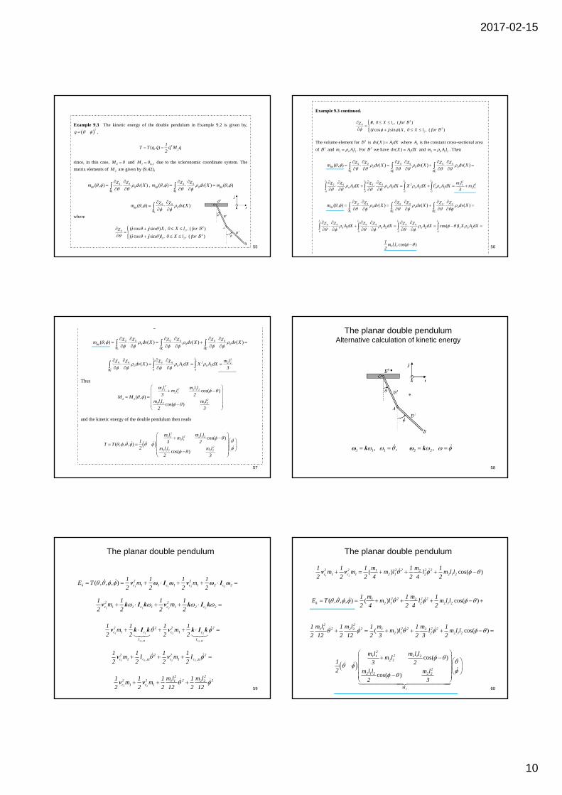
Example 9.3 The kinetic energy of the double pendulum in Example 9.2 is given by,
Tq ,
( , ) T2
1T T q q q M q
2
since, in this case, 0M 0 and 1 1 2M 0 due to the scleronomic coordinate system. The
matrix elements of 2M are given by (9.42),
( , ) ( )q q0m dv X
0B, ( , ) ( ) ( , )q q
0m dv X m
0B
( , ) ( )q q0m dv X
0B
where
( cos sin ) , , ( )
( cos sin ) , , ( )
1q 1
21 2
X 0 X l for
l 0 X l for
i j
i j
Example 9.3 continued.
, , ( )
( cos sin ) , , ( )
1q 1
22
0 X l for
X 0 X l for
0
i j
The volume element for 1 is ( ) 1dv X A dX where 1A is the constant cross-sectional area
of 1 and 1 0 1 1m A l . For 2 we have ( ) 2dv X A dX and 2 0 2 2m A l . Then
( , ) ( ) ( ) ( )1 20 0
q q q q q q0 0 0m dv X dv X dv X
0B B B
1 2 1 2l l l l 2
q q q q 2 2 21 10 1 0 2 0 2 1 0 2 2 1
0 0 0 0
m lA dX A dX X A dX l A dX m l
3
( , ) ( ) ( ) ( )1 20 0
q q q q q q0 0 0m dv X dv X dv X
0B B B
cos( )1 2 2 2l l l l
q q q q q q0 1 0 2 0 2 1 0 2
0 0 0 0
A dX A dX A dX l X A dX
cos( )2 1 2
1m l l
2 56
2
( , ) ( ) ( ) ( )1 20 0
q q q q q q0 0 0m dv X dv X dv X
0B B B
( )2 2
20
l l 2q q q q 2 2 2
0 0 2 0 2
0 0
m ldv X A dX X A dX
3
B
Thus
cos( )( , )
cos( )
221 1 2 1 2
2 1
2 2 22 1 2 2 2
m l m l lm l
3 2M Mm l l m l
2 3
and the kinetic energy of the double pendulum then reads
cos( )
( , , , )
cos( )
221 1 2 1 2
2 1
22 1 2 2 2
m l m l lm l
1 3 2T T2 m l l m l
2 3
57
The planar double pendulumAlternative calculation of kinetic energy
, ,1 1 1 ω k , 2 2 ω k
58
59
( , , , )1 1 2 2
2 2k c 1 1 c 1 c 1 2 c 2
1 1 1 1E T m m
2 2 2 2 v ω I ω v ω I ω
1 1 2 2
2 2c 1 1 c 1 c 1 2 c 2
1 1 1 1m m
2 2 2 2 v k I k v k I k
, ,1 1 2 2
2 2 2 2c 1 c zz c 1 c zz
1 1 1 1m I m I
2 2 2 2 v v
, ,
1 1 2 2
c zz c zz1 2
2 2 2 2c 1 c c 1 c
I I
1 1 1 1m m
2 2 2 2 v k I k v k I k
The planar double pendulum
1 2
2 22 2 2 21 1 2 2c 1 c 1
m l m l1 1 1 1m m
2 2 2 12 2 12 v v
60
( ) cos( )1 2
2 2 2 2 2 21 2c 1 c 1 2 1 2 2 1 2
m m1 1 1 1 1m m m l l m l l
2 2 2 4 2 4 2 v v
The planar double pendulum
( , , , ) ( ) cos( )2 2 2 21 2k 2 1 2 2 1 2
m m1 1 1E T m l l m l l
2 4 2 4 2
( ) cos( )2 2
2 2 2 2 2 21 1 2 2 1 22 1 2 2 1 2
m l m l m m1 1 1 1 1m l l m l l
2 12 2 12 2 3 2 3 2
cos( )
cos( )
2
221 1 2 1 2
2 1
22 1 2 2 2
M
m l m l lm l
1 3 22 m l l m l
2 3

2017-02-15
11
( , , ) ( )T0 1 2
1T T t q q M M q q M q
2
The kinetic energy
T1 2 n n 1q q q q
( , )0 0 00M M t q m
( , ) ,
11 12 1n
21 22 2n n n T2 2 2 2
n1 n2 nn
m m m
m m mM M t q M M
m m m
( , ) 1 n1 1 01 10 02 20 0n n0M M t q m m m m m m
61
where the matrix elements, , , , ,...,klm k l 0 1 n , are defined by
( , ) ( )q q00 00 0m m t q dv X
t t
0B
( , ) ( ) , ,...,q q0k 0k 0 k0k
m m t q dv X m k 1 nt q
0B
( , ) ( ) , , ,...,q qkl kl 0 lkk l
m m t q dv X m k l 1 nq q
0B
Mass matrix elements
62
63
( , , ) T1T T t q q q Mq
2
( , )
00 01 0n
0 110 11 1n
T1 2
n0 n1 nn
m m m1M M m m m2M M t q
1M M
2 m m m
Mass matrix elements
( ) , T0 2 n n 1 1 0q q q q q t
Proposition 9.7 The generalized inertial forces may be written a ra ta ga
k k k kQ Q Q Q
where
( )ra 2 2k k k
d T TQ
dt q q
is the relative inertial force,
( )ta 01k k k
TTQ
t q q
is the transport inertial force and
2n
ga j1 1k j k k
j 1
T TQ q
q q q
is the gyroscopic inertial force.
The kinetic energy
64
The kinetic energy
Proposition 9.8 The transport inertial force may be written
n
ta i0 00k k
i 1
m m1Q
t 2 q
Proposition 9.9 The gyroscopic inertial force may be written
n
ga jk kj
j 1
Q g q
where
2 2
0 j0k1 1kj j k k j j k
mmT Tg
q q q q q q
The so-called gyroscopic matrix ijg g is thus skew-symmetric, i.e. Tg g . 65
Proposition 9.10 The relative inertial force may be written
,
n n nra i i j ikik ki kij
i 1 i j 1 i 1
mQ m q C q q q
t
where
( ), , , ,...ij kjkikij j k i
m mm1C i j k 1 n
2 q q q
The kinetic energy
66

2017-02-15
12
Lagrange’s equations
( ) , ,...,ta ga i e2 2k k k kk k
T TdQ Q Q Q 0 k 1 n
dt q q
,
( , , )n
k l T2 2 kl 2
k l 1
1 1T T t q q m q q q M q
2 2
67
Corollary 9.2 Lagrange’s equations are given by T cif i e
2q M Q Q Q
where
( ( ) ) ( ( )) ( )cif T t T 02 2 2 1 1 MM M M M M1 1Q q q q skew
q 2 q t q 2 t q
is the complementary inertia force and
i i i i1 2 nQ Q Q Q and e e e e
1 2 nQ Q Q Q
Lagrange’s equations
cif T iT eT2M q Q Q Q
68
69
The complementary inertia force in a scleronomiccoordinate system
( ( ) )T t2 2M M1q q
q 2 q
( ( ) ) ( ( )) ( )cif T t T 02 2 2 1 1 MM M M M M1 1Q q q q skew
q 2 q t q 2 t q
, 0 1 1 nM 0 M 0
cif2n n n 1 n
M0 Q 0
q
Box 9.3 Kinetic energy and inertial forces
0 1 2T T T T
0 00
1T m
2 , ( )
nk
1 0k k0k 1
1T m m q
2
, ,
nk l
2 klk l 1
1T m q q
2
( )q q00 0m dv X
t t
0B
, ( )q q0k 0k
m dv Xt q
0B
( )q qkl 0k l
m dv Xq q
0B
cif T iT eT
2M q Q Q Q
( ( ) ) ( ( ))cif T t T2 2 2 1M M M M1Q q q q skew
q 2 q t q
( )01 MM1
2 t q
Summary
70
Regular coordinates
The system of generalized coordinates , , ... , 1 2 nq q q q , ( , ; )qx t q X is said to be regular
if for fixed ( , )t q
( , , ; ) , , ,...,n
q k kq k
k 1
t q w X w 0 X w 0 k 1 nq
w 0B
Proposition 9.12 The system of generalized coordinates is regular if and only if the massmatrix 2M is positive definite.
71
Example 9.2 Underlying, in our discussion, is the assumption that we may use different sets of generalized coordinates for the configuration space of the multibody. The choice of coordinates must be decided by the engineer. For instance, for a single particle P we may use Cartesian coordinates ( )x, y, z or spherical coordinates ( , , )r related by, cf. example 9.1,
sin cos
sin sin
cos
r
r
r
x
y
z
Let ( )e e ex y z denote the RON-basis corresponding to the Cartesian coordinate system
with origin O. The transplacement of the particle may be written ( )( ; ) 3
q Ox P x e e e x y zx,y,z x y z, x, y, z
Then
q
exx
, q
eyy
, q
ezz
and thus the Cartesian coordinate system is regular. In spherical coordinates
72

2017-02-15
13
Example 9.4 continued.
sin cos sin sin cosq
r
e e ex y z ,
cos cos cos sin ( sin )qzr r r
e e ex y ,
( sin sin ) sin cosq r r
e ex y
and
sin , ( )q q q 2r 0 rr
, ,
This spherical coordinate system is thus a regular coordinate system. However in this case
3 is not equal to the whole of 3 .
73
Example 9.5 The coordinate system adopted for the double pendulum in Example 9.2 is regular since, for fixed ( ) , ,
q q1 2w w
( cos sin ) , , ( )
cos sin ) (cos sin ) , , ( )
1 11
1 2 21 2
Xw 0 X l for
l w Xw 0 X l for
i j 0
i j i j 0
1 2w w 0
74
Coordinate changes
( , ; ) ( , ; )q qt q X t q X
0B
tB
X
x
nq nqq̂
1q
- : nq space 1q
q
- : nq space q
75
...T1 2 nq q q q ... ,
T1 2 nq q q q
( , ( ); ) ( , ( ); ) q qx t q t X t q t X X 0B
Coordinate change
q q ˆ( , )q q t qCoordinate change:
ˆ ˆ ˆ( , ), 1q q t q q q
q̂
76
Coordinate changesVirtual velocity fields
( , , ; )n
q jq j
j 1
t q w X wq
w w( , , ; )n
q kq k
k 1
t q w X wq
w w
T1 2 n nw w w w
ˆ knk j
jj 1
qw w
q
T1 2 n nw w w w
q̂w w
q
ˆ ˆ kn n
j
q q
q q
Jacobian:
Component change:
77
Proposition 9.13 If the - coordinate systemq is regular then the - coordinate systemq is
regular if and only if
ˆ
det( )q
0q
Proposition 9.14
ˆ ˆq q
q qt q
* q̂Q Q
q
where Q may be any of eQ , iQ or aQ .
Coordinate changes
78

2017-02-15
14
79
Coordinate changes
ˆ ˆˆ( ) ( , ( )) , ,...,
k knk j
jj 1
q qq t q t q t q q k 1 n
t q
ˆ ˆq qq q
t q
ˆ( ) ( ) ( )
knq q qe
j 0 0 0j j k jk 1
qQ da X dv X da X
q q q q
Pn b Pn00 0BB B
ˆ ˆ ˆ( ) ( ( ) ( ))
k k kn n nq q q e
0 0 0 kk j k k j jk 1 k 1 k 1
q q qdv X da X dv X Q
q q q q q q
b Pn b0 00B BB
Covariant and contravariant vectors
q̂q q
q
q̂w w
q
* q̂Q Q
q
Covariant vector:
Contravariant vector:
a i eQ Q Q 0
Lagrange’s equations are on covariant form:
ˆ( )n 1
q0
t
80
ˆ( )a i e a i e q
Q Q Q Q Q Qq
Theorem 9.2 Lagrange’s equations are invariant under a regular coordinate transformation,i.e. a i e a i eQ Q Q 0 Q Q Q 0
Invariance of Lagrange’s equations
Lagrange’s equations are invariant under regular changes of the configurationcoordinates!
81
Box 9.4: Regular coordinates and change of coordinates
ˆ( , )q q t q
ˆdet( )
q0
q
ˆ ˆq q
q qt q
, * q̂Q Q
q
Summary
82
The rigid part
O
Inertial frame
Ax
ω
Ax
tB
( , ; ) ( , ) ( , )( ), q A At q X x t q t q X X X R 0B
; ( ), , ,...,def
Tk k
ax k 0 1 nq
R
ω R
;
nk
kk 0
q
ω ω ,
nk
A A kk 0
q
x x
,
defA
A k k
x
q
x
83
( )A Ax x x x ω
The rigid part
;
nk
kk 0
q
ω ω ,
nk
A A kk 0
q
x x
84
Corollary 9.3
, ;
defA
A k A k kq
x
x x
and ; , , ,...,k kk 0 1 n
q
ω
ω

2017-02-15
15
Proposition 9.18 The mass matrix elements of the kinetic energy for a rigid part may bewritten ; ; ; ; ; ; ; ;( ) , , , ,...,kl A k A l A k l Ac A l k Ac k A lm m k l 0 1 n x x x ω p x ω p ω I ω
where A
I is the inertia tensor of the rigid part . For a scleronomic coordinate system
00m 0 , , ,...,0km 0 k 1 n
The rigid part: The mass matrix
(( ) ( ) ( )) ( )t
2A A A Ax x x x x x dv x
I 1B
; ;A kl k A lm x 0 ω I ω
Inertia tensor:
85
Corollary 9.4 By taking A c , the centre of mass, the following matrix elements areobtained ; ; ; ;kl c k c l k c lm m x x ω I ω
The rigid part: The mass matrix
86
The double pendulum
;k kq
ω
ω
;A
A k kq
x
x
; ; ; ; ; ; ; ;( ) , , , ,...,kl A k A l A k l Ac A l k Ac k A lm m k l 0 1 n x x x ω p x ω p ω I ω
87
The double pendulum
2 ω k
; ; ; ; ; ; ; ; ; ;( )1 1 1 1 1 1 1 1 1 1 1 1 1 1 1 1kl O k O l O k l Oc O l k Oc k O l k O lm m x x x ω p x ω p ω I ω ω I ω
1 ω k
O x 0
; ; ; ; , , ,2 2 2 2 2 2 2kl c k c l k c lm m k l x x ω I ω
88
Example 9.6 Let us calculate the mass matrix of the double pendulum in Example 9.2 by using the formula (9.73) for a rigid part. For part 1 and with A O we have, since O x 0
, 1 ω k and ;
11
ω
ω k ,
; ; ,
21 1 1 1 1 1 1 1
O O O zz
m lm I
3 ω I ω k I k
Furthermore ;
1 ω 0 and then
1 1 1m m m 0
For part 2 we may use the expression in Corollary 9.4 where 2 ω k and then
;
22
ω
ω 0 . Moreover
( cos sin ) ( cos sin )2 2c 1
ll
2 x i j i j ; ( cos sin )2
c 1l x i j
89
and then
; ; ; ;2 2 2 2 2 2 2 2
c c 2 c 2 1m m m m l x x ω I ω
Next
; ; ; ; ; ;2 2 2 2 2 2 2 2 2
c c 2 c c c 2m m m m x x ω I ω x x
( cos sin ) ( cos ) sin ) cos( )2 2 1 21 2
l m l ll m
2 2 i j i j
Finally, with ;
22
ω
ω k ,
; ; ; ; ( cos sin ) ( cos sin )2 2 2 2 2 2 2 2c c 2 c 2
l lm m m
2 2 x x ω I ω i j i j
,
2 2 2 22 22 2 2 2 2 2 2 2c c zz
m l m l m l m lI
4 4 12 3 k I k
90
2017-02-15
16
Summarizing,
21 1 21 1
2 1
m lm m m m l
3 , cos( )1 2 22 1
lm m m m l
2 , 2
2 2 2m lm
3
and
cos( )( , )
cos( )
221 1 2 1 2
2 1
2 2 22 1 2 2 2
m l m l lm l
3 2M Mm l l m l
2 3
91
The rigid part: The internal force
Proposition 9.16 For a rigid part the generalized internal force is zero, i.e. , , ,...,i
kQ 0 k 1 n
92
( )qik k
Q dv Xq
E
S0B
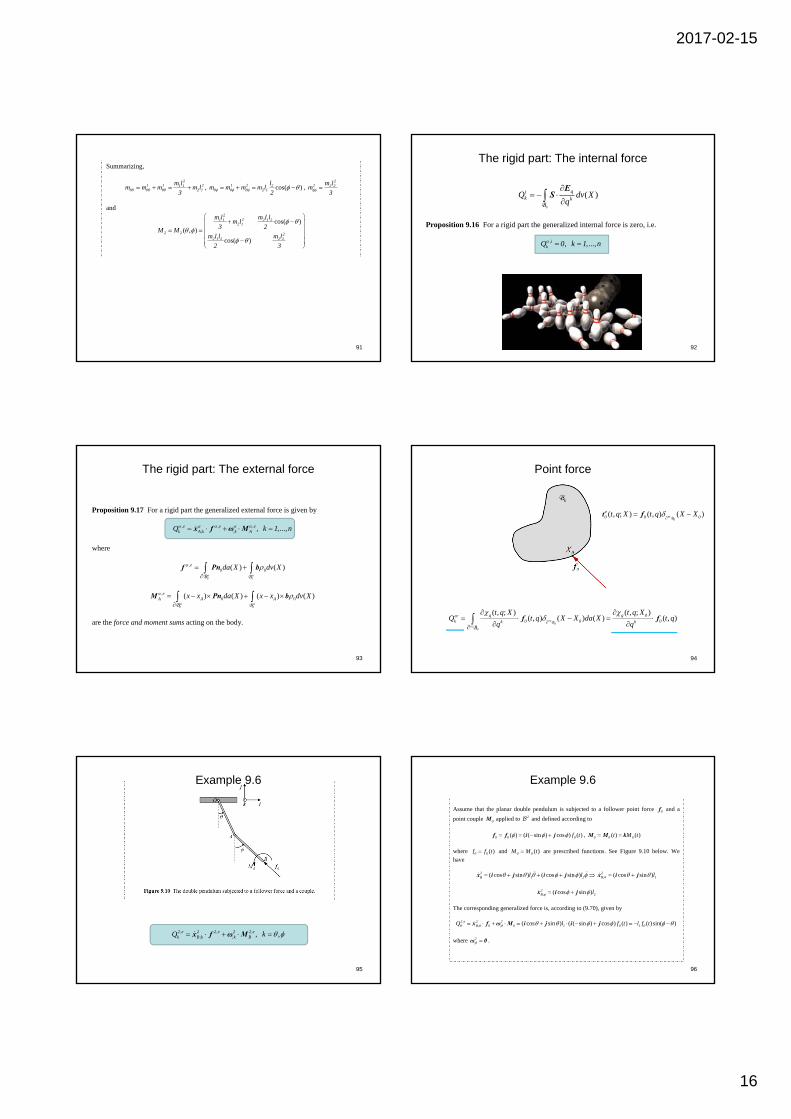
The rigid part: The external force
93
Proposition 9.17 For a rigid part the generalized external force is given by , , ,
; ; , ,...,e e ek A k k AQ k 1 n x f ω M
where
,0 0( ) ( )e da X dv X
f Pn b0 0BB
,0 0( ) ( ) ( ) ( )e
A A Ax x da X x x dv X
M Pn b0 0BB
are the force and moment sums acting on the body.
94
Point force
( , ; ) ( , ; )( , ) ( ) ( ) ( , )ec
0ec
0
q q 0eck 0 0 0k k
t q X t q XQ t q X X da X t q
q q
f fB
B
( , ; ) ( , ) ( )ec0
e0 0 0t q X t q X X
t f
B
Example 9.6
, , ,; ; , ,2 e 2 2 e 2 2 e
k B k k BQ k x f ω M
95
Example 9.6
96
Assume that the planar double pendulum is subjected to a follower point force 0f and a
point couple 0M applied to 2 and defined according to
( ) ( ( sin ) cos ) ( )0 0 0f t f f i j , ( ) ( )0 0 0t M t M M k
where ( )0 0f f t and ( )0 0M M t are prescribed functions. See Figure 9.10 below. We
have
( cos sin ) ( cos sin )2B 1 2l l x i j i j ; ( cos sin )2
B 1l x i j
; ( cos sin )2B 2l x i j
The corresponding generalized force is, according to (9.70), given by
,; ; ( cos sin ) ( ( sin ) cos ) ( ) ( ) sin( )2 e 2 2
B 0 0 1 0 1 0Q l f t l f t x f ω M i j i j
where ;
2 ω 0 .
2017-02-15
17
97
Example 9.6, cont’d
,
; ; ( cos sin ) ( ( sin ) cos ) ( ) ( ) ( )2 e 2 2B 0 0 2 0 0 0Q l f t M t M t x f ω M i j i j k k
We have thus found that
, ( ) sin( )2 e1 0Q l f t , , ( )2 e
0Q M t or , ( ) sin( ) ( )e 2 e1 0 0Q Q l f t M t
O
A
B
0f 0M
O i
j
k
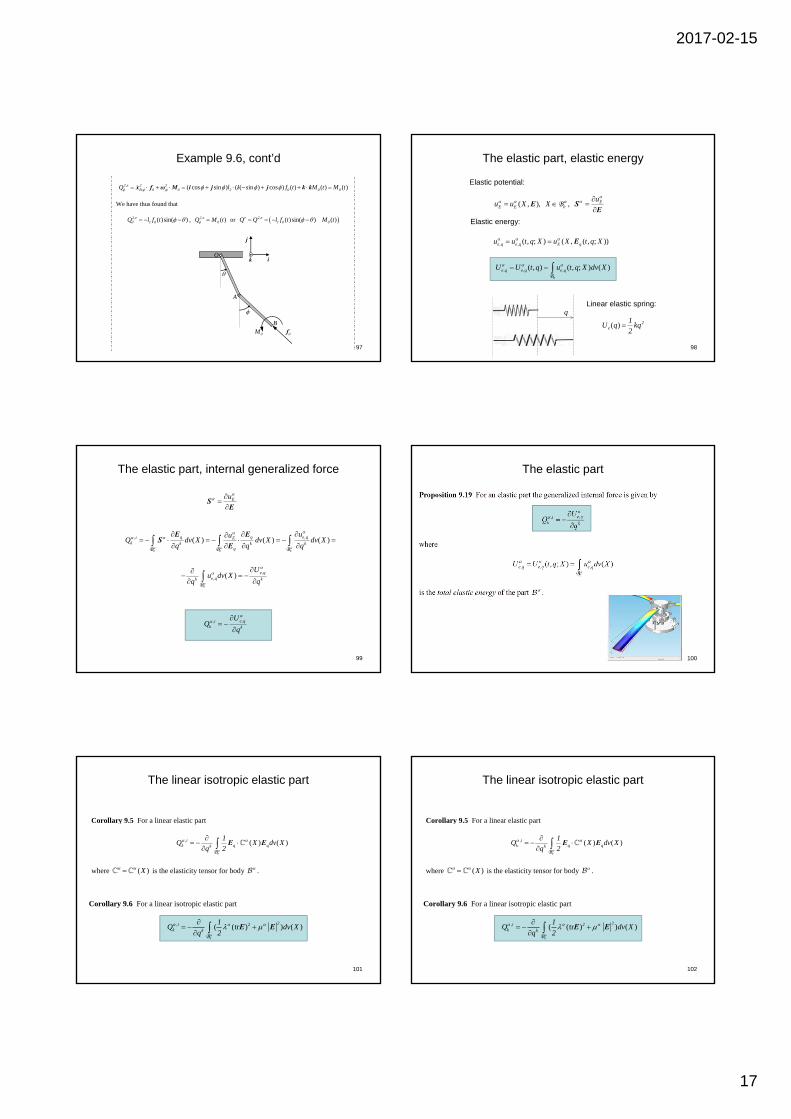
The elastic part, elastic energy
( , ), , EE E
uu u X X
E S
E0B
, , ( , ; ) ( , ( , ; ))e q e q E qu u t q X u X t q X E
q
( ) 2e
1U q kq
2
Linear elastic spring:
, , ,( , ) ( , ; ) ( )0
e q e q e qU U t q u t q X dv X B
98
Elastic potential:
Elastic energy:
The elastic part, internal generalized force
Eu
SE
99
,, ( ) ( ) ( )q q e qi Ek k k k
q
uuQ dv X dv X dv X
q q q
E E
SE
0 0 0B B B
,, ( )
0
e qe qk k
Uu dv X
q q
B
,, e qik k
UQ
q
The elastic part
100
Corollary 9.6 For a linear isotropic elastic part
, ( (tr ) ) ( )2i 2
k k
1Q dv X
q 2
E E0B
The linear isotropic elastic part
Corollary 9.5 For a linear elastic part
, ( ) ( )ik q qk
1Q X dv X
q 2
E E0B
where ( )X is the elasticity tensor for body .
101
Corollary 9.6 For a linear isotropic elastic part
, ( (tr ) ) ( )2i 2
k k
1Q dv X
q 2
E E0B
The linear isotropic elastic part
Corollary 9.5 For a linear elastic part
, ( ) ( )ik q qk
1Q X dv X
q 2
E E0B
where ( )X is the elasticity tensor for body .
102
2017-02-15
18
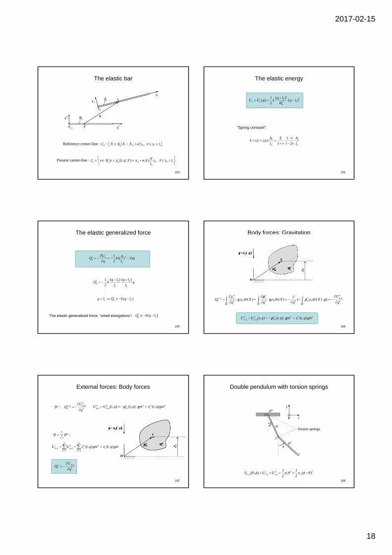
The elastic bar
, ( , ; ) ( )Present center-line : t t q O 1 0 0 00
0 lq
x x t q X x t s sl
eC B
, Reference center-line : 00 O 1 0 0 00 lX X X s s e0C B
103
The elastic energy
( )( ) ( )
220
e e 020
q l1U U q k q l
2 4l
( ) 0 0
0 0
A AE 1k 2
l 1 1 2 l
”Spring constant”:
104
The elastic generalized force
(( ) )i 2eq
0
U 1 qQ k 1 q
q 2 l
( ) ( )i 0 0q
0 0
q l q l1Q k q
2 l l
( )iq 0Q k q l The elastic generalized force, ”small elongations”:
( )i0 q 0q l Q k q l
105
Body forces: Gravitation
,, ( ) ( ) ( ( ) )q q g qgk 0 0 q 0k k k k
UQ dv X dv X dv X
q q q q
pg g p g
0 0 0B B B
, , ( , ) ( , ) ( , )g q g q Oc cU U t q t q m z t q gm p g
106
External forces: Body forces
,g qgk k
UQ
q
,, g qgk k
UQ
q
, , ( , ) ( , ) ( , )g q g q Oc cU U t q t q m z t q gm p g
, , ( , ) ( , )N N
g q g q c c1 1
U U z t q gm z t q gm
1:
N
:
107
Double pendulum with torsion springs
Torsion springs
, , ,( , ) ( )1 2 2 2e q e q e q 1 2
1 1U U U
2 2
108
2017-02-15
19
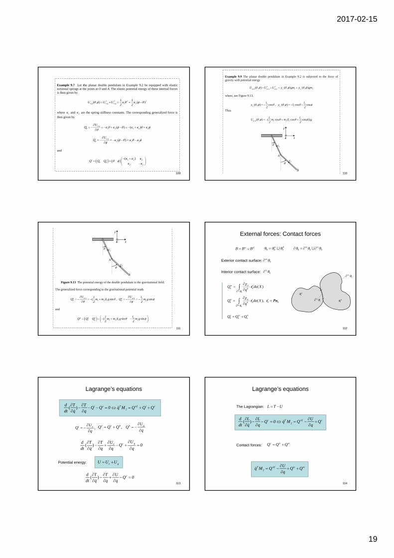
Example 9.7 Let the planar double pendulum in Example 9.2 be equipped with elastic torsional springs at the joints at O and A. The elastic potential energy of these internal forces is then given by
, , ,( , ) ( )1 2 2 2e q e q e q 1 2
1 1U U U
2 2
where 1 and 2 are the spring stiffness constants. The corresponding generalized force is
then given by
, ( ) ( )e qi1 2 1 2 2
UQ
, ( )e qi2 2 2
UQ
and
( )1 2 2i i i
2 2
Q Q Q
109
Example 9.9 The planar double pendulum in Example 9.2 is subjected to the force of gravity with potential energy
, , ,( , ) ( , ) ( , )1 2
1 2g q g q g q c 1 c 2U U U y gm y gm
where, see Figure 9.13,
( , ) cos1
1c
ly
2 , ( , ) cos cos
2
2c 1
ly l
2
Thus
, ( , ) ( cos ( cos cos ))1 2g q 1 2 1
l lU m m l g
2 2
O
A
B
1c
2c
i
j
k
110
Figure 9.13 The potential energy of the double pendulum in the gravitational field. The generalized force corresponding to the gravitational potential reads
, ( ) sing qg1 2 1
U 1Q m m l g
2
, , sing qg 2
2
U lQ m g
2
and
( ) sin sing g g 21 2 1 2
l1Q Q Q m m l g m g
2 2
O
A
B
1c
2c
i
j
k
111
External forces: Contact forces
( )ec
qec ek 0k
Q da Xq
t0B
ec 0B
ec ic0 0 0B B B
ic 0B
( ), qic i ik 0 0 0k
ic
Q da Xq
t t Pn
0B
c ec ick k kQ Q Q
0 0 0 B B B
Exterior contact surface:
Interior contact surface:
tB
ict B
tB
ect B
112
113
Lagrange’s equations
,i eUQ
q
( ) i e T cif i e2
d T TQ Q 0 q M Q Q Q
dt q q
,e c bQ Q Q gb UQ
q
( ) gceUUd T T
Q 0dt q q q q
e gU U U
( ) cd T T UQ 0
dt q q q
Potential energy:
114
c ic ecQ Q Q
( ) c T cif c2
d L L UQ 0 q M Q Q
dt q q q
L T U
Lagrange’s equations
The Lagrangian:
T cif ic ec2
Uq M Q Q Q
q
Contact forces:

2017-02-15
20
Exercise 4:14
115
Exercise 4:14 Solution
Configuration coordinates: ,x
116
117
Exercise 4:14 Solution
( ), ,
Placement: ( , ; ) ( ) ,
( sin ) ( cos ),
0 1O OP O 1 0 0
0
0 2q O OB BP O 1 0 BP
0 0 3O OP O 1 0 2
aX
x x l P 0 X ll
x P x x l P
x x l l l P
p e
p p e p
p e e
x
x xx
Exercise 4:14 Solution
( , ; ) , q P Pt
0 x
( , ; ) , , q 0 11 0
0
XP P 0 X l
l
e x
x
Partial derivatives of the transplacement:
( , ; ) , q 0 2 31P P
e x
x
118
, ,
( , ; ) ,
cos sin ,
10
q 2
0 0 31 2
P 0 X l
P P
l l P
0
0
e e
x
119
Exercise 4:14 Solution
The material velocity:
( , , , ; ) q q qPt
x x x x x
x
, ,
,
cos sin ,
0 11 0
0
0 21
0 0 0 31 1 2
XP 0 X l
l
P
l l P
00 e
0 e 0
0 e e e
x
xx
, ,
,
( cos ) sin ,
0 11 0
0
0 21
0 0 31 2
XP 0 X l
l
P
l l P
e
e
e e
x
xx
Exercise 4:14 Solution
( , , , ) (( cos ) ( sin ) )2 2 2 2 2C c B c
1 1 1 1T T m m m l l m
2 2 2 2 v v x x x x
cos( ( ) cos )
cos
T
c2 2 2c 2
m m ml1 1m m 2ml ml
ml ml2 2
x x
x x
Kinetic energy:
cos
cosc
2 2
m m mlM
ml ml
Mass matrix:
120
, 0 1 1 2M 0 M 0
2017-02-15
21
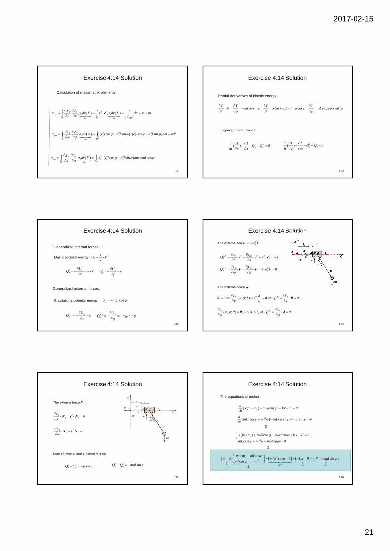
Exercise 4:14 Solution
( ) ( )q q 0 0xx 0 1 1 0 c
2 3dm dm
m dv X dv X dm m mx x
e e 0 0B B
Calculation of massmatrix elements:
( ) ( cos sin ) ( cos sin )q q 0 0 0 0 20 1 2 1 2
3dm
m dv X l l l l dm ml
e e e e
0B
( ) ( cos sin ) cosq q 0 0 0x 0 1 1 2
3dm
m dv X l l dm mlx
e e e
0B
121
Exercise 4:14 Solution
T0
xsin
Tml
x cos 2Tml ml
x( ) cosc
Tm m ml
xx
Partial derivatives of kinetic energy:
( ) i ed T TQ Q 0
dt
x xx x( ) i ed T T
Q Q 0dt
Lagrange’s equations:
122
Exercise 4:14 Solution
Generalized internal forces:
i eUQ k
x xx
2e
1U k
2 x
i eUQ 0
Elastic potential energy:
Generalized external forces:
Gravitational potential energy: cosgU mgl
, ge g UQ 0
x x, singe g U
Q mgl
123
Exercise 4:14 Solution
The external force :01 FF e
, qe F 0 0OC1 1Q F F
pF F e ex x x
, qe F 0OC1Q F 0
pF F 0 e
124
The external force :R
,( , ; )q q0 e R1
0
XX 0 P Q 0
l
e 0 Rxx
x x
,( , ; ) , q qe R0P 0 X l Q 0
0 Rx
125
Exercise 4:14 Solution
The external force :1N
q 01 1 1 0
N e N
x
q1 1 0
N 0 N
i eQ Q k F x x x sini eQ Q mgl
Sum of internal and external forces:
A O cm
k
l
0
mg
F B 01e
02e
R
1N 2N
1 2
3
C
x 0l
Exercise 4:14 Solution
( cos ) sin sin
2dml ml ml mgl 0
dt
x x
( ( ) cos )c
dm m ml k F 0
dt x x
cos
sin sincos
i ecif
2
c 22
q Q QQM
m m mlml 0 k 0 F mgl
ml ml
x x
( ) cos sin
cos sin
2c
2
m m ml ml k F 0
ml ml mgl 0
x xx
The equations of motion:
126
2017-02-15
22
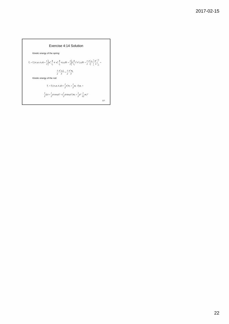
127
( , , , ) ( )00 0ll l 2 3
0 0 2 2 0s s 1 1 0 0 2
0 0 0 00 0 0
1 X X 1 X 1 XT T dX dX
2 l l 2 l 2 l 3
e e
xx x x x x
Exercise 4:14 Solution
Kinetic energy of the spring:
2 20 0 0l m1 1
2 3 2 3
x x
Kinetic energy of the rod:
( , , , ) 2r r c r r c r
1 1T T m
2 2 v ω I ω x x
(( cos ) ( sin ) )2 2 2 2r r
1 l l 1 1m m l
2 2 2 2 12 x