DEVELOPMENT OF A SIMPLE DIAGNOSIS TOOL FOR ETECTING LOCALIZED ROUGHNESS FEATURES

yung Suk Lee, M.S.

epartment of Civil and Environmental Engineerinter of Excellence

05 February 2009

D

arim Chatti, Ph.D. KImen Zaabar, M.S. H

Michigan State University D ng

Pavement Research Ce

Final Report Project RC-15

Technical Report Documentation Page

1. Report No. RC-1505

2. Government Accession No.

3. MDOT Project Manager Mike Eacker

5. Report Date February, 2009

4. Title and Subtitle Development Of A Simple Diagnosis Tool For Detecting Localized Roughness Features 6. Performing Organization Code

7. Author(s) Karim Chatti, Associate professor Imen Zaabar, Graduate Research assistant

8. Performing Org. Report No.

10. Work Unit No. (TRAIS) 11. Contract No.

9. Performing Organization Name and Address Pavement Research Center of Excellence Michigan State University Department of Civil and Environmental Engineering, 3546 Engineering Building, Michigan State University East Lansing, MI 48824-1226

11(a). Authorization No. 13. Type of Report & Period Covered

Final Report 12. Sponsoring Agency Name and Address Michigan Department of Transportation Construction and Technology Division P.O. Box 30049 Lansing, MI 48909

14. Sponsoring Agency Code

15. Supplementary Notes This project corresponds to Task B of the project Effect Of Michigan Multi-Axle Trucks On Pavement Distress and Profile. 16. Abstract The collection of distress data from video imaging of the pavement surface can provide the location and type of many distresses. However, it cannot provide useful information about some distress features such as the magnitude of faulting, breaks and curling in concrete pavements. This report describes a simple tool to extract such information through the use of the raw profile data. Different methods were used in the study, including wavelets, time frequency and discrete methods. The discrete elevation difference method (DED) was selected for faulting and breaks detection, and the discrete slope method (DS) was selected for curling detection. To test the validity of the analysis, surveys were conducted on different sites in Michigan. The new tool was able to detect the magnitude of faulting, breaks and curling with an R2 of 0.97 and standard error (SE) of 0.25 mm. The localization was also highly accurate (R2 =0.99). The results indicate that the methods described above can capture relevant information about these roughness features with reasonable accuracy. 17. Key Words Detection, Localized roughness features, Faulting, Breaks, Curling

18. Distribution Statement No restrictions. This document is available to the public through the Michigan Department of Transportation.

19. Security Classification - report Unclassified

20. Security Classification - pageUnclassified

21. No. of Pages 74

22. Price

DISCLAMER

This document is disseminated under the sponsorship of the Michigan Department of

Transportation (MDOT) in the interest of information exchange. MDOT assumes no

liability for its contents or use thereof.

The contents of this report reflect the views of the contracting organization, which is

responsible for the accuracy of the information presented herein. The contents may not

necessarily reflect the views of MDOT and do not constitute standards, specifications,

or regulations.

TABLE OF CONTENTS

TABLE OF CONTENTS .............................................................................................................. i LIST OF FIGURES ...................................................................................................................... ii LIST OF TABLES ....................................................................................................................... iv CHAPTER 1- INTRODUCTION................................................................................................ 1

1.1 BACKGROUND........................................................................................................................ 1 1.2 RESEARCH OBJECTIVES.......................................................................................................... 1 1.3 ORGANIZATION ...................................................................................................................... 2

CHAPTER 2- PAVEMENT DISTRESS AND ROUGHNESS IDENTIFICATION ............ 3 2.1 INTRODUCTION....................................................................................................................... 3 2.2 LITERATURE REVIEW ............................................................................................................. 3 2.3 REVIEWING MDOT’S DATA SOURCE..................................................................................... 4 2.4 EVALUATING OTHER METHODS FOR ANALYZING A PROFILE................................................. 5

2.4.1 Pavement Faulting ......................................................................................................... 5 2.4.1.1 Methods for Identifying Joint/Crack Faulting ........................................................ 8 2.4.1.2 Discrete Elevation Difference method with threshold.......................................... 12

2.4.2 Pavement Breaks.......................................................................................................... 20 2.4.3 Slab Curling................................................................................................................. 21

2.4.3.1 Methods for Identifying Slab Curling................................................................... 21 2.4.3.2 Discrete Slope Method.......................................................................................... 26

2.5 FIELD TRIALS....................................................................................................................... 29 2.5.1 Field Trips.................................................................................................................... 29 2.5.2 Results .......................................................................................................................... 31

CHAPTER 3- DEVELOPMENT OF A PROFILE-BASED DIAGNOSTIC TOOL FOR IDENTIFYING SURFACE DISTRESSES .............................................................................. 34

3.1 INTRODUCTION..................................................................................................................... 34 3.2 USER MANUAL FOR DISTRESS DETECTION TOOL................................................................. 34

3.2.1 Import/Export Windows ............................................................................................... 34 3.2.1.1 ERD files............................................................................................................... 34 3.2.1.2 Import window...................................................................................................... 39 3.2.1.3 Export window...................................................................................................... 39

3.2.2 Faulting Detection Window ......................................................................................... 39 3.2.3 Breaks Detection Window............................................................................................ 42 3.2.4 Curling Detection Window .......................................................................................... 43

CONCLUSION ........................................................................................................................... 45 REFERENCES............................................................................................................................ 46 APPENDIX A: Field Trials Data............................................................................................. A-1

SITE 1....................................................................................................................................... A-1 SITE 2....................................................................................................................................... A-5 SITE 3....................................................................................................................................... A-9 SITE 4..................................................................................................................................... A-14

Appendix B: Repeated Measurements.................................................................................... B-1 SITE 2....................................................................................................................................... B-1 SITE 3....................................................................................................................................... B-2

i

LIST OF FIGURES Figure 2.1 Faulting detected by Pathway’s procedure.................................................................... 5

Figure 2.2 Theoretical samples from faulting of slabs ................................................................... 6

Figure 2.3 Faulting from actual profile........................................................................................... 6

Figure 2.4 Components of the created dummy profile ................................................................... 7

Figure 2.5 Dummy profile ............................................................................................................. 7

Figure 2.6 Faulting of dummy profile............................................................................................. 8

Figure 2.7 Daubechies 3 wavelet analysis ...................................................................................... 9

Figure 2.8 Profile and slope .......................................................................................................... 10

Figure 2.9 Profile and curvature ................................................................................................... 10

Figure 2.10 Profile and discrete elevation difference ................................................................... 10

Figure 2.11 Discontinuities detected by slope and adaptive filtering........................................... 11

Figure 2.12 Discontinuities detected by curvature and adaptive filtering .................................... 11

Figure 2.13 Discontinuities detected by discrete elevation difference and adaptive filtering ...... 11

Figure 2.14 Detected faulting from the discrete elevation difference method ............................. 13

Figure 2.15 Detected faulting from the slope method .................................................................. 13

Figure 2.16 Detected faulting from the Haar wavelet method...................................................... 14

Figure 2.17 Detected faulting from the db2 wavelet method ....................................................... 14

Figure 2.18 Detected faulting from the coif1 wavelet method ..................................................... 15

Figure 2.19 Detected faulting from the sym2 wavelet method..................................................... 15

Figure 2.20 Detected faulting using discrete elevation difference method & adaptive filtering.. 16

Figure 2.21 Detected faulting from the slope method & adaptive filtering.................................. 16

Figure 2.22 Detected faulting from the Haar wavelet method & adaptive filtering ..................... 17

Figure 2.23 Detected faulting from the db2 wavelet method & adaptive filtering....................... 17

Figure 2.24 Detected faulting from the coif1 wavelet method & adaptive filtering..................... 18

Figure 2.25 Detected faulting from the sym2 wavelet method & adaptive filtering .................... 18

Figure 2.26 Faulting at a crack and its maximum value ............................................................... 19

Figure 2.27 Different scenarios of recording a fault after filtering............................................... 19

Figure 2.28 Fault detection algorithm........................................................................................... 20

Figure 2.29 Breaks ........................................................................................................................ 21

Figure 2.30 Breaks detection algorithm........................................................................................ 22

ii

Figure 2.31 Created curling and extracted curling........................................................................ 22

Figure 2.32 Created curling and extracted curling........................................................................ 23

Figure 2.33 Wigner-Ville joint time frequency distribution of the dummy profile...................... 24

Figure 2.34 Pseudo Wigner-Ville joint time frequency distribution of the dummy profile ......... 25

Figure 2.35 Smoothed Pseudo Wigner-Ville time frequency distribution of dummy profile ...... 25

Figure 2.36 Created curling and extracted curling with DS ......................................................... 26

Figure 2.37 Original and filtered profiles ..................................................................................... 27

Figure 2.38 Detection of local maxima of the slope function....................................................... 27

Figure 2.39 Curling detection algorithm....................................................................................... 28

Figure 2.40 Correlation analyses for Site 2 (a) magnitude (b) location........................................ 31

Figure 2.41 Correlation analyses for Site 3 (a) magnitude (b) location........................................ 32

Figure 2.42 Correlation analyses for Site 4 (a) magnitude (b) location........................................ 32

Figure 2.43 Raw profile with severe curling (Site 1).................................................................... 32

Figure 2.44 Filtered profile and curling magnitude ...................................................................... 33

Figure 3.1 Set up of the security level .......................................................................................... 35

Figure 3.2 Security alert message ................................................................................................. 35

Figure 3.3 Main window............................................................................................................... 36

Figure 3.4 Localized roughness window ...................................................................................... 36

Figure 3.5 Short Header for an ERD File with Text Data. ........................................................... 38

Figure 3.6 Example of required headings for the input files ........................................................ 38

Figure 3.7 Import file window...................................................................................................... 39

Figure 3.8 Export results window................................................................................................. 39

Figure 3.9 Fault detection results window.................................................................................... 40

Figure 3.10 faulting detection window displaying the original profile ........................................ 41

Figure 3.11 Fault results summary and distribution window ....................................................... 41

Figure 3.12 Breaks detection results window............................................................................... 42

Figure 3.13 curling detection results window............................................................................... 43

Figure 3. 14 curling detection window displaying the original and the filtered profile .............. 44

iii

LIST OF TABLES Table 2.1 Number of Pavement Sections1 for Verification of the Roughness Diagnosis Tool ... 29

Table 2.2 Definition of Severity Level ......................................................................................... 29

Table 2.3 Summary of measured faults in I69.............................................................................. 30

Table 2.4 Summary of measured faults in each section................................................................ 30

Table 3.1 Summary of records in an ERD file header.................................................................. 37

iv

CHAPTER 1 INTRODUCTION

1.1 BACKGROUND

Michigan’s PMS system collects pavement surface distresses (type, extent, and severity) from video images of the pavement surface bi-annually. The raw profile is measured by a high speed profilometer. Surface distresses and profile data are used to compute Distress Index (DI) and Ride Quality Index (RQI), for a minimum segment length of 0.1 mile. The bi-annual change of the pavement’s DI is included in a performance model to estimate the pavement’s Remaining Service Life (RSL).

Road roughness indices such as the International Roughness Index (IRI) and RQI are useful as indicators of the level of pavement serviceability. Each of these summary roughness statistics offers a convenient index for monitoring the trend of pavement roughness deterioration with time. However, they do not retain the actual contents of pavement surface roughness. Such detailed roughness information may be useful for maintenance operations, and detection of roughness features. The collection of distress data from video images of the pavement surface can provide the location and type of many distresses. However, because video images of pavement surface are two-dimensional, they cannot quantify pavement surface characteristics. Therefore, such images cannot provide useful information about roughness features, such as their magnitude. Failure to include specific roughness features in Pavement Management Systems (PMS) has the following negative impacts on system performance:

(1) The analysis may overestimate the RSL of the pavement; (2) The system process may not select the most appropriate fix to extend pavement

life. 1.2 RESEARCH OBJECTIVES

The objectives of this research study are: 1. Developing a profile-based diagnosis method for distinguishing non-identifiable

surface distresses from video imaging that have one of the following impacts: a) Significant impact on pavement structural integrity b) Significant impact on pavement roughness, as determined from RQI c) Significant cause of pavement deterioration

2. Developing a window-based software system that can detect the presence of certain distresses from the profile and then tabulate these distresses, as identified in objective (1).

1

1.3 ORGANIZATION This final report contains 3 chapters including this introductory chapter. Chapter 2 investigates methods of identifying certain pavement distresses through the use of profile data. Finally, Chapter 3 presents the user’s manual for the new profile-based diagnostic tool for identifying surface distresses.

2

CHAPTER 2 PAVEMENT DISTRESS AND ROUGHNESS

IDENTIFICATION 2.1 INTRODUCTION

MDOT annually collects the distress and profile data in order to calculate the Distress Index (DI) and Ride Quality Index (RQI). The distress data from the video imaging of the pavement surface may provide where certain distresses are present. However, some information about the distress such as the magnitude of faulting or curling can not be extracted from the two dimensional video images. The objective of this analysis presented in this chapter is to extrapolate such information through the use of the profile database. 2.2 LITERATURE REVIEW

Although a lot of information on profile analyses is documented, they are mostly based on an index type (i.e. IRI, RQI, etc.) of analyses. Few studies were found under the subject of diagnosing/localizing distresses from the actual profile data.

De Pont (1999) introduced wavelets to be used for identifying the local features of

the profile. The method he suggested localizes the features of the profile in terms of short, medium and long wavelengths. However, the method does not identify the individual distresses that are present. De Pont also discussed the usefulness of the wavelets in terms of compressing the profile data for storage. From his example, the profile data was compressed into only 5% of the size of the original signal, and the reconstructed signal had a maximum difference of 0.003m (0.12 in) in comparison to the original signal.

Byrum (2001) developed an algorithm that picks up the “imperfection” zone from

the profile of rigid pavements. These imperfection zones are then separated from the slab region, and then the curvature index is calculated for the slab region. The identification of the imperfection zone is done by calculating the curvature of the profile and applying a threshold on the curvature. The curvature variation threshold (CVT) is calculated by the following equation:

[ ]7819.31446.18405.0 )48(06631.0)24(00665.0)06(03242.00213.0121 CVStDevCVStDevCVStDevCVT −++−=

(0.003 < CVT < 0.015 ft-1) R2 = 0.81 Where: 06CVStDev = Standard deviation of the 6〃 curvatures in 500 ft. profile, 1/ft *1000

24CVStDev = Standard deviation of the 24〃 curvatures in 500 ft. profile, 1/ft *1000

3

48CVStDev = Standard deviation of the 48〃 curvatures in 500 ft. profile, 1/ft *1000

Fernando and Bertrand (2002) used moving average filters to detect localized roughness. The points where the deviations from the averaged profile are large are the rough areas. However, this method does not identify the actual distresses.

Attoh-Okine (2003) introduced wavelet analysis as a method of profile analysis.

He mentions that using wavelet analysis; the profile may be studied beyond the index type of analyses.

Chang et al. (2005) identified localized roughness based on the Texas Department

of Transportation Specification Tex-1001-S. First, each elevation point from the two longitudinal profiles (left and right wheel paths) is averaged to produce a single averaged wheel path profile. Then, the resulted profile is placed on a 7.6 m (25 ft), centered-moving average filter. The difference between the average wheel path profile and the 7.6m-moving average filtered profile for every profile point is computed. Deviations greater than 3.8 mm (0.15 in) are considered a detected area of localized roughness. Positive deviations are considered as "bumps" and negative ones as "dips". However, this method does not identify the distress type. 2.3 REVIEWING MDOT’S DATA SOURCE

MDOT’s current contractor for video and laser data collection is Pathway Services Inc. The Pathway laser profiler collects the elevation of the profile at every 0.75 inches (the sampling interval). These measurements are averaged every 3 inches and recorded (the recording interval). These profile samples are taken for left and right wheel paths and the center of the lane. For each of the longitudinal profiles, the differences in height 3 inches apart are taken and the variance of the differences of the heights is calculated for each point. Then, a moving average filter is applied to the calculated variances and compared with the actual elevation differences. The base length for the variance and moving average calculations is 20 ft (10 ft before and after). This procedure is repeated for all three longitudinal profiles (left and right wheel paths and the center of the lane), and if the elevation difference is greater than the averaged variance for all three longitudinal profiles, then the point is classified as faulting. Figure 2.1 shows a dummy profile generated by the research team (see section 2.4 for details of the dummy profile) and the faulting detected by the Pathway’s procedure. Note that this is only for a single longitudinal profile. The procedure detects the presence of faulting but in a wide range rather than at a certain point.

The research team was able to access the profiles that were collected by MDOT

during 1993-99. These profiles were collected with a sample interval of 3 in, which is the interval still in use by MDOT. However, the sections corresponding to the profiles do not provide the research team with the distress locations.

4

0

1Fa

ultin

g (y

es=1

, no=

0)

-2

0

2

4

6

Elev

atio

n (in

)

2

Distance (ft)

-4

8

100 150 200 250 300 350 400-6

Faulting(y/n) Dummy profile

Meanwhile, the research team had used the profile and distress data from LTPP w sections in Michigan. These data were extracted from the were collected using a sample interval of 1 in. Prior to being

ntered

Since the research team did not have access to the recent (at the time of this project) profile data collected by the Pathway profilometer, old profiles collected by MDOT during 1993-1999 and the LTPP profiles were studied. 2.4.1 Pavement Faulting

Faulting and curling of slabs are the major rigid pavement distresses that need to be identified from a surface profile because they cannot be determined from video imaging. Faulting of the joints/cracks is defined as the difference in elevation of the two adjacent slabs before and after the joint/crack, as shown in Figure 2.2. Theoretically, when the samples the difference in elevation should appear in two adjacent sam les. However, from the MDOT profile data the faulting does not appear in two adjacent points. Faulting of the slabs in the actual

Figure 2.1 Faulting detected by Pathway’s procedure

SPS-2 sections including a feTPP database. The profiles L

e into the database, the collected samples are passed through a 300 ft high-pass filter to eliminate the gradual, long wavelengths. After that, the profiles are reported with a sample interval of 6 in. The distresses such as faulting of LTPP sections can be identified from the database. However, the database does not contain information about curling of rigid pavement slabs. 2.4 EVALUATING OTHER METHODS FOR ANALYZING A PROFILE

of the profile are collected over a faulted joint/crack,p

5

profile appears at several sample points, asvaluate faulting is that the differences in elevation be taken from the raw profile before

applying the moving average filter. Another way will be explained later.

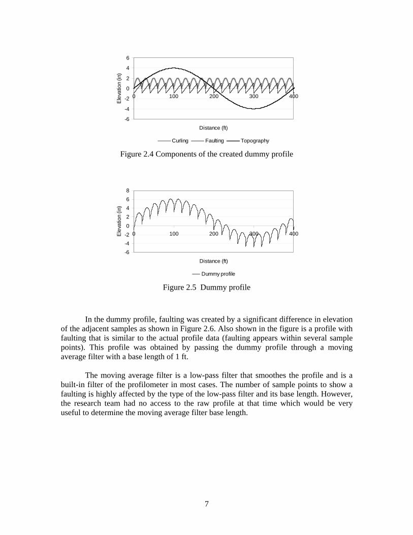
In order to explain such phenomenon, the research team performed a study using a dummy profile. The dummy profile wa ollowing:

• Long wave sinusoid that represents the topography of the site. • Short wave sinusoid that represents the curling of the slabs. •

ampling interval used by MDOT.

shown in Figure 2.3. Thus, the best way to e

Sampled Points

Direction of traffic

Approach Slab

Leave Slab

Figure 2.2 Theoretical samples from faulting of slabs

-3

-2

-1

0

1

2

0 100 200 300 400 500

Distance (ft)

Ele

vatio

n (in

)

Figure 2.3 Faulting from actual profile

s cre d to include the fate

Discontinuous line that represents the faulting of the joints/cracks. Figure 2.4 shows the components of the dummy profile listed above. The dummy

profile is the sum of these three functions and is shown in Figure 2.5. A sample interval of 3 inches was used to meet the current s

6

-6

-4

-2

0

2

4

6

0 100 200 300 400

Distance (ft)

Ele

vatio

n (in

)

Curling Faulting Topography Figure 2.4 Components of the created dummy profile

-2

468

0 100 200 300 400El

n (in

)

0

2

evat

io

-6-4

Distance (ft)

Dummy profile Figure 2.5 Dummy profile

In the dummy profile, faulting was created by a significant difference in elevation of the a

he moving average filter is a low-pass filter that smoothes the profile and is a built-in

th.

djacent samples as shown in Figure 2.6. Also shown in the figure is a profile with faulting that is similar to the actual profile data (faulting appears within several sample points). This profile was obtained by passing the dummy profile through a moving average filter with a base length of 1 ft.

T filter of the profilometer in most cases. The number of sample points to show a

faulting is highly affected by the type of the low-pass filter and its base length. However, the research team had no access to the raw profile at that time which would be very useful to determine the moving average filter base leng

7

0

0.5

15 17 19 21 23 25Distance (ft)

1

Ele

v

1.5

22.5

3

atio

n (in

)

Dummy profile Averaged profile Figure 2.6 Faulting of dummy profile

2.4.1.1 Methods for Identifying Joint/Crack Faulting

Four methods were studied for identifying the faulting from a profile; (1) Discrete Elevation Difference ( method, (3) Discrete

urvature (DC) method and (4) Wavelet analysis method. The DED method takes the elevation difference of the two discrete sample points. These two points would be the two adjacent points if there were no filters applied to the profile that is being analyzed. However, because the faulting appears in several points in a filtered profile, the two points are not adjacent but exist with some distance apart. This distance would be dependent on the type and the base length of the filter applied to the profile.

The DS method is used to detect discontinuities in digital image processing. It is

similar to the DED method in the sense that it takes the difference of the elevation heights. But the difference is that the slope (difference in elevation) is taken from the adjacent sample points. The DC method is similar to the DS method other than that it takes the curvature (2nd derivative) of the profile.

Wavelet analysis is a popular met mpression and multi-resolution

analysis of discrete signals. It d several signals of different scale. The term ‘scale’ here allows the user to see the signal in different scales along with time or distance.

However, all the analyses herein are based on the averaged profile and not the raw

profile except for the artificially generated dummy profile. It is again because the research team did not have the raw profile data at that time.

Figure 2.7 shows an example of the wavelet analysis of a profile from LTPP

section (20-0201). “D1” and “D2” may be treated as noise since they are decomposed of high frequency contents. “D3” and “D4” may provide useful information depending on the type of the mother wavelet used. The highlighted locations in Figure 2.7 might have potential of faulting or cracking since they show high variations in the decomposed signal.

DED) method, (2) Discrete Slope (DS) C

hod for cogiecomposes a ven signal into

is related to frequency. Thus, it

8

The wavelets used were haar wavelets, da echies (db) wavelets, symlets (sym), and coiflets (coif).

ub

Once the method is decided, then it is important to decide on the threshold. Two

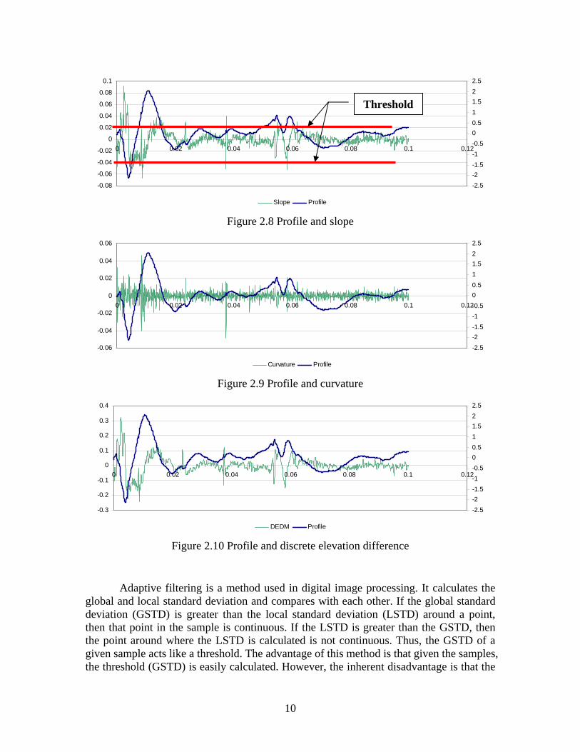
possible methods are suggested: (1) Threshold, and (2) Adaptive Filtering. Thresholds may simply be applied on the slope, curvature, DED, and on wavelets. Figure 2.8 shows an example of threshold applied on the slope with a value of 0.3. With this threshold, all the locations that have slopes in between -0.3 and 0.3 are considered to be continuous. Although it is not shown in figures 2.9 and 2.10, similar thresholds may be applied to the curvature and DED. Unlike the example of threshold shown in figure 2.7, deciding on a threshold value is not a simple problem. Sufficient profile data was needed to decide on a reliable threshold.

Figure 2.7 Daubechies 3 wavelet analysis

9

10

-0.08

-0.06

-0.04

-0.02

0

0.02

0.04

0 0.02 0.04 0.06 0.08 0.1 0.12

-2.5-2-1.5-1-0.500.511.50.06

0.08 22.50.1

Slope Profile Figure 2.8 Profile and slope

-0.06

0.1 0.12

-2-1.5-1-0.500.51

-0.04

-0.020 0.02 0.04 0.06 0.08

0

0.02

0.04

0.06

1.522.5

-2.5

Curvature Profile

Figure 2.9 Profile and curv

ature

-0.3

-0.2

-0.1

0

0.1

0.3

0.4

0 0.02 0.04 0.06 0.08 0.1 0.12

-2.5-2-1.5-1-0.500.511.522.5

0.2

DEDM Profile Figure 2.10 Profile and discrete elevation difference

Adaptive filtering is a method used in digital image processing. It calculates the global and local standard deviation and compares with each other. If the global standard deviation (GSTD) is greater than the local standard deviation (LSTD) around a point, then that point in the sample is continuous. If the LSTD is greater than the GSTD, then the point around where the LSTD is calculated is not continuous. Thus, the GSTD of a given sample acts like a threshold. The advantage of this method is that given the samples, the threshold (GSTD) is easily calculated. However, the inherent disadvantage is that the

Threshold

threshold is dependent on the numdoes not clearly point out the locations of

11

ber of sampled points and if the signal is very noisy it discontinuities (figure 2.12). Figures 2.11

through 2.13 show the discontinuities on the profile using the slope, curvature and DEDM, respectively, along with the adaptive filtering.

-0.3

-0.2

-0.1

0

0.1

0.2

0.3

0 0.01 0.02 0.03 0.04 0.05 0.06 0.07 0.08 0.09 0.1

Distance (mile)

Faul

ting

(in)

-2.5-2-1.5-1-0.500.511.522.5

Elev

atio

n (in

)

DEDM Profile Figure 2.13 Discontinuities detected by discrete elevation difference and adaptive

filtering

-0.3

-0.2

-0.1

0

0.1

0.2

0.3

0.4

0 0.01 0.02 0.03 0. 0 0.06 0.07 0.08 0.09 0.1

istan )

Faul

ting

(in

-0.3-0.25-0.2

-0.15-0.1

-0.050

0.050.1

0.150.2

0.25

0 0.01 0.02 0.03 0.04 0.05 0.06 0.07 0.08 0.09 0.1

istance (mile)

Faul

ting

(in

D

)

-2.5-2-1.5-1-0.500.511.522.5

Elev

atio

n (in

)

Slope Profile

slope and adaptive filtering

Figure 2.11 Discontinuities detected by

04

D

.05

ce (mile

)

-2.5-2-1.5-1-0.500.511.522.5

Elev

atio

n (in

)

Curvature Profile Figure 2.12 Discontinuities de re and adaptive filtering tected by curvatu

section with the highest faul

was mfaultings that were detected frommm for DEDM and slope m2.20 through 2.25 show the samthreshowavelet m 2.4.

with threshold for detecting faulting at joint/

12

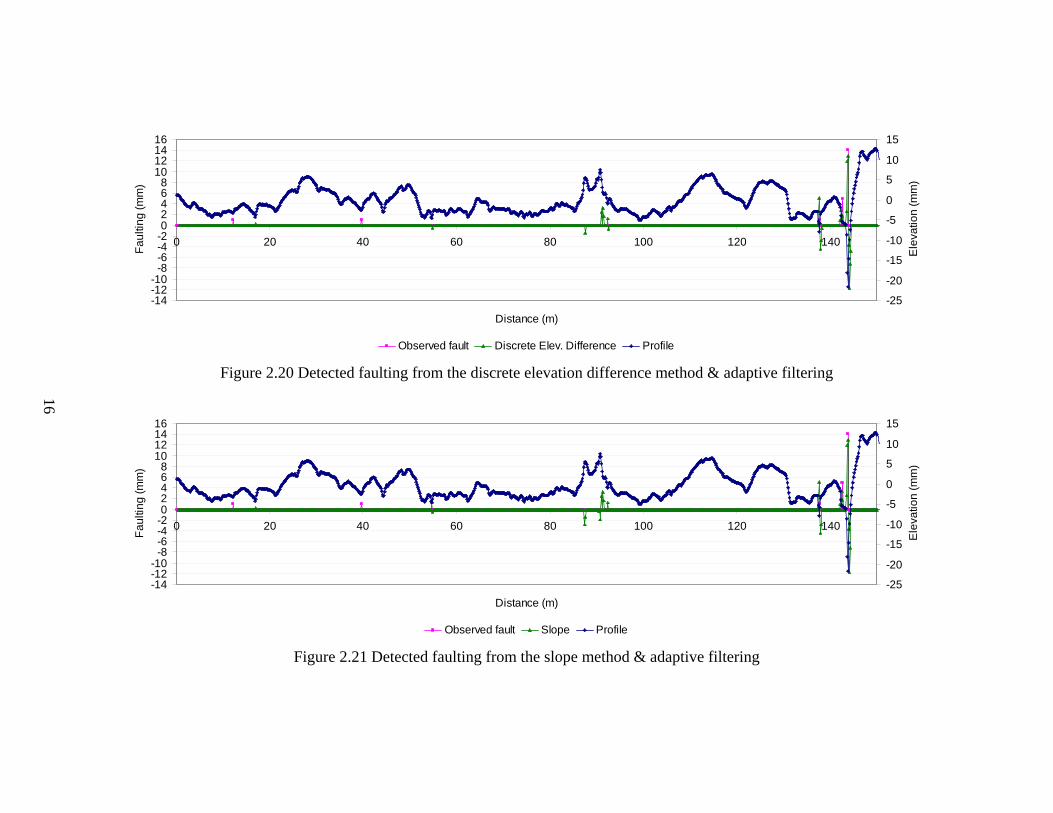
The methods mentioned above were tested using LTPP profile data. The LTPP ting (14 mm) was selected.

Figures 2.14 through 2.19 show a profile of an LTPP section with faulting that easured from the field with an accuracy of ±1 mm. The figures also show the

the methods described above and a threshold value of 1 ethod while 0.5 mm was used for D1’s of wavelets. Figures

e methods but with adaptive filtering instead of theld. The discrete elevation difference method detected the faulting better than the

ethods in terms of location and magnitude.

1.2 Discrete Elevation Difference method with threshold

For the reasons mentioned above, the research team has selected the DED method iscrete elevation

difference method consists of computing the difference in elevation between points at a given interval. Theoretically, when the samp llected over a faulted joint/crack, the difference in elevation should t samples. However, as shown before, the faulting of the slab in ears at several sample points (Figure 2.6). As seen before, the elevat ery 0.75 in [sampling interval] and recorded at every 3 in [recording interval]. Consequently, when the difference in elevation is computed, each lt/cra represented by a range of differences. Thus, the largest absolute valu um) for each range of differences was taken as the fault magnitudefrom aulting is calculated points, three different values of the fault mwhether the distance to the fault is a multiple of interval:

agnitude, [ Figure 3 (a)];

agnitude, [Figure 3 (b) and (d)]; agnitude [Figure 3 (c)].

In order to resolve this problem, it was d

between the points that are 6 in apart (±3 in. of the point of interest). The algorithm for the fault detection method is described in Figure 2.28.

figure 2.27, if the f

(1) Exact m(2) 75% of the exact m(3) 50% of the exact m

crack. To summarize, the d

les of the profile are coappear in two adjacen

the raw profile appion is collected at ev

faue (local maxim

(Figure 2.26). However, as it can be seen based on the elevation difference of adjacent

agnitude can be obtained, depending on the reco

ecided to take the difference in elevation

ck is

rding

0123456789

101112131415

0 20 40 60 80 100 120 140Distance (m)

Ele

vatio

n (m

m)

-25-20-15-10-5051015

Faul

ting

(mm

)

Observed fault Discrete Elev. Difference Profile Figure 2.14 Detected faulting from the discrete elevation difference method

02468

10121416

0 20 40 60 80 100 120 140Distance (m)

Faul

ting

(mm

)

-25-20-15-10-5051015

Ele

vatio

n (m

m)

Observed fault Slope Profile Figure 2.15 Detected faulting from the slope method

13

0123456789

101112131415

0 20 40 60 80 100 120 140Distance (m)

Ele

vatio

n (m

m)

-25-20-15-10-5051015

Faul

ting

(mm

)

Observed fault Haar Profile

0123456789

101112131415

0 20 40 60 80 100 120 140Distance (m)

Ele

vatio

n (m

m)

-25-20-15-10-5051015

Faul

ting

(mm

)

Observed fault db2 Profile Figure 2.17 Detected faulting from the db2 wavelet method

Figure 2.16 Detected faulting from the Haar wavelet method

14

Observed fault coif1 Profile Figure 2.18 Detected faulting from the coif1 wavelet method

Observed fault sym2 Profile Figure 2 etected faulting from the sym2 wavelet method

0123456789

101112131415

0 20 40 60 80 120 140Distance (m)

mm

)

-25-20-15-10-5051015

Faul

ting

(mm

)

20 40 60 80 120 140Distance (m)

-25-20-15-10-5051015

Faul

ting

(mm

)

100

100

.19 D

00123456789

101112131415

Ele

vatio

n (

Ele

vatio

n (m

m)

15

-1420

-8-6-4-202468

10121416

0

-1-1

2 60 80 100 120 140

Distance (m)

Faul

ting

(mm

)

-25

-20

-15

-10

-5

0

5

10

15

Ele

vatio

n (m

m)

0 40

Obse faultrved Discrete Elev. Difference Profile e d faulting fr he discrete elevation difference method & adaptive filtering

-14-12-10

-8-6-4

Figur 2.20 Detecte om t

-202468

10121416

0 20 40 60 80 100 120 140

Distance (m)

Faul

ting

(mm

)

-25

-20

-15

-10

-5

0

5

10

15

Ele

vatio

n (m

m)

Observed fault Slope Profile 21 Detected faulting from the slope method & adaptive filtering Figure 2.

16

-14-12-10

-8-6-4-202468

10121416

0 20 40 60

Distan

80

e (m)

100 120 140

c

Faul

ting

(mm

)

-25

-20

-15

-10

-5

0

5

10

15

Ele

vatio

n (m

m)

Observed fault Haar Pro u d fau a avelet aptive filter

file

method & adFig re 2.22 Detecte lting from the H ar w ing

-14-12-10

-8-6-4-202468

10121416

0 20 40 60 8

Distance (m

0 120 140

)

Faul

ting

(mm

)

-25

-20

-15

-10

-5

0

5

10

15

Ele

vatio

n (m

m)

100

Observed fault db2 Profile gure d fa b2 wavelet m ptive filtering ethod & adaulting from the d 2.23 DetecteFi

17

-1-1-1

Fa

420

-8-6-4-202468

10121416

0 20 40 60 80 100 120 140

Distance (m)

ultin

g (m

m)

-25

-20

-15

-10

-5

0

5

10

15

Ele

vatio

n (m

m)

Observed fault coif1 Profile Figure 2.24 ected faulting from the coif1 wavelet method & adaptive filtering

Det

-14

Observed fault sym2 Profile Figure 2.25 Detected faulting from the sym2 wavelet method & adaptive filtering

-1-1

1111

Faul

ting

(mm

)

20

-8-6-4-2024680246

0 20 4 60 80 100 120 140

Distance (m)-25

-20

-15

-10

-5

0

5

10

15

Ele

vatio

n (m

m)

0

18

-0.6000

-0.4000

-0.2000

0.0000

0.2000

0.4000

0.6000

0.8000

14600 14610 14620 14630 14640 14650 14660 14670 14680 14690 14700

Distance (inch)

Faul

ting

(inch

)

-8

-6

-4

-2

0

2

4

6

8

10

Elev

atio

n (in

ch)

Faulting average value Profile Figure 2.26 Faulting at a crack and its maximum value

(a) (b)

3 in.

3 in. 3 in.

3 in

(c) (d) Figure 2.27 Different scenarios of recording a fault after filtering

19

2.4.2 Pavement Breaks

h a negative fault and ends with a positive fault. The research team has decided that the distance between the two opposite faults should not exceed 3ft (Figure 2.29). This threshold could be updated according to MDOT needs.

Before detecting breaks, different steps are followed. First, differences in

elevation are computed. This step is the same as the fault detection method. Second, if the sign of two successive faults is different, the method checks the distance between them: if the distance is less than 3ft, it is considered break; otherwise, there is no break. The algorithm for the breaks detection is described in Figure 2.30.

Figure 2.28 Fault detection algorithm

Read Original Profile

Calculate ∆yn = yn-yn+2

Calculate local maximum (∆yn)Lmax

(∆yn)Lmax >T No Yes

No Faulting Faulting (∆yn)Lmax

End

A pavement break is a broken portion of the pavement section that starts wit

20

F

2.4.3 Slab Curling

Curling is the distortion of a bending of the edges. This distortionan unsupported edge or corner whichcurling is evident at any early age. Ino

2.4.3.1 Methods for Identifying S

Several methods were studieprofile. The methods studied were;Joint Time Frequency (JTF) analysisMethod. The moving average of the the moving average filters are lowpassing the profile into the filters.

The Gaussian Band-Pass Filt

Fourier Transform (FFT) algorithm. FFT to the profile and then applyingshows the artificial curling used in thextracted using the GBPF method. T

Figure 2.32 shows the curling

three different wavelet analyses; db1

f time.

+

igure 2.29 B

slab into a cu can lift the e can crack w other cases,

lab Curling

d to extract t (1) Gaussia, (3) waveletprofiles is no-pass filters

er extracts ceThus, the cu the filter to te dummy prhe curling w

profiles ext0, sym8, and

21

-

<3ft

reaks

rved shape by upward or downward dges of the slab from the base leaving hen heavy loads are applied. Sometimes, slabs may curl over an extended period

he curling of the slabs from the dummy n Band-Pass Filter (GBPF) method, (2) analysis method, and (4) Discrete Slope t critical for identifying curling because and do not eliminate the curling after

rtain frequency contents from the Fast rling can be extracted after performing he transformed profile. Figure 2.31 ofile along with the curling that was as extracted with a phase lag.

racted from the dummy profile, using coif5 wavelets.

Figure 2.30 Breaks detection algorithm

-2-1.5

-1-0.5

00.5

11.5

2

0 20 40 60 80 100

elev

atio

n (in

distance (ft)

)

curling fft_bandpass

Figure 2.31 Created curling and extracted curling

Read Original Profile

Calculate ∆yn = yn-yn+2

Calculate local maximum (∆yn)Lmax

(∆yn)Lmax >T No Yes

No Faulting Faulting (∆yn)Lmax

End

Breaks (∆yn)Lmax

Sgn((∆yn)Lmax) ≠ Sgn((∆yn+1)Lmax) No

Yes

Dist((∆yn+1)Lmax) - Dist((∆yn)Lmax) < 3ft No

Yes

22

-1.5

-1

-0.5

0

0.5

1

1.5

0 20 40 60 80 100

distance (ft)

elev

atio

n (in

)

curling db10 (a) Extracted curling of the dummy profile using db10 wavelets

-1.5

-1

-0.5

0

0.5

1

1.5

0 20 40 60 80 100

elev

atio

n (in

)

distance (ft)

curling sym8 (b) Extracted curling of the dummy profile using sym8 wavelets

-1.5

-1

-0.5

0

0.5

1

1.5

ion

(in)

0 20 40 60 80 100

distance (ft)

elev

at

curling coif5 (c) Extracted curling of the dummy profile using coif5 wavelets

Figure 2.32 Created curling and extracted curling

Joint time frequency analysis was performed on the dummy profile and the LTPP

profile (section 19-0217). The joint time frequency analysis calculates the frequency energy distribution along with the time/distance. Thus, it overcomes the weakness of the Fourier Transform which only provides the overall frequency content but time information.

Although, the joint time frequency analysis method is powerful for electrical and

mechanical signals, it was not efficient for the analysis of pavement profiles. Figures 2.33 through 2. 5 s PWVD), and 3 how the Wigner-Ville Distribution (WVD), Pseudo WVD (

23

Smoothed Pseudo WVD (SPWVD) of the dummy profile. As it can be seen from the ourier spectrum –placed at the left hand side of the time frequency distribution- the ajor energy is concentrated in relatively low frequency components.

The Discrete Slope (DS) method is used to detect discontinuities in digital image

rocessing. It is similar to the DED method in the sense that it takes the difference of the levation heights. But the difference is that the slope (difference in elevation) is taken om the adjacent sample points. Figure 2.36 shows a simulated profile and the orresponding slope.

It can be seen from figures 2.31 through 2.35 that the GBPF method seems to

ork better than wavelet and time-frequency methods. However, this method produces a hase lag or time shift which could affect the localization. The DS method produces same rder of error in magnitude but more accurate in localization.

Fm

pefrc

wpo

Figure 2.33 Wigner-Ville joint time frequency distribution of the dummy profile

24

Figure 2.34 Pseudo Wigner-Ville joint time frequency distribution of the dummy profile

Figure 2.35 Smoothed Pseudo Wigner-Ville joint time frequency distribution of the

dummy profile

25

2.4.3.2

ince we are looking for discontinuities in the slope of the profile, the discrete slope (

the difference in elevation. But the difference is that the slope (difference in elevation divided by the distance between the points) is taken from e topography has an impact on the curling m(300 ft long cut-off wavelength) was applied. ro cro-curling, a low-pass filter (5 ft short cut-off wavelength) was applied. Figure 2.37 shows the results after each step.

of approa s have been used for removing the long-wave topography f profile moving avera 2-pole Butterw h, 4-pole But orth (Sayers et al., 1996), etc.). The principles of several filtering techniques have been discussed in the pavement smoothness literature (Chang et al., 2005). In this analysis, we have used the Bu hness detection algorithms. These re superior since e the following stics

d 9 Sm

ecified cut-off frequencies

Schematic Profile with Daytime Curling

-4 -2 0

2

4

6

0 20 40 60 80 100 120 140 160

Distance

Elevation Schematic Profile with Nighttime Curling

-4

-2

0

2

4

6

0 20 40 60 80 100 120 140 160

Elevation

Distance

Slope of Profile

-0.1 -0.05

0 0.05 0.1

Slope

Slope of Profile

-0.05

0

0.05

0.1Slope

-0.10 2 4 6 8 100 120 140 160 20 40 60 80 100 120 140 160

Distance Distance

Figure 2.36 Created curling and extracted curling with DS

Discrete Slope Method

SDS) method was identified as a method to detect slab curling. This method has

been used in signal and image processing for its capability to detect discontinuities. It is similar to the DED method in the sense that it takes

the adjacent sample points. It is noted that thagnitude detection. To filter out the topography, a high-pass filter

Then, to eliminate the effect of profile ughness and mi

A number

rom the measuredche

(e.g. ge, ort terw

tterworth filters before implementing the specific roug filters a they hav characteri

(Orfani is, 19 6):

• ooth response at all frequencies • Monotonic decrease from the sp

26

•

• alf-power frequency that corresponds to the specified cut-off frequencies

Maximal flatness, with the ideal response of unity in the passband and zero otherwise. H

-30

-200 20 40 60 80

Raw Profile long w avelength f iltering short w avelength f iltering

-90

-80

-70

-60

-50

-40

Distance (m)

Ele

vatio

n (m

m)

Figure 2.37 Original and filtered profiles

ted (Figure 2.38). The algorithm for the curling bed in Figure 2.39.

Since a 2-pole Butterworth filter add a phase lag to the filtered profile, a 4-pole Butterworth was needed. Finally, to compute curling, differences in elevation between the point that corresponds to the local maximum of the slope function and the next point where the slope function is zero is compudetection is descri

-2

-1.5

-0.5

0

0.5

1

1.5

2

20 40 60 80

Distance (m)

ope

(mm

/m)

Figure 2.38 Detection of local maxima of the slope function

Local maximum

0

-1

sl

27

Figure 2.39 Curling detection algorithm

Read Original Profile

Calculate ∆yn = (yn+1- yn)/( dn+1- dn)

Calculate local maximum locations

of the slope (Lmax)

End

Long wavelength cut off

Short wavelength cut off

Calculate local zero locations of the

Slope (L0) (∆yn)L0

Calculate curling elevation (∆yn)L0-(∆yn)Lmax

28

2.5 FIELD TRIALS

Different methods were used in the study, including wavelets, time-frequency and discrete methods. The discrete elevation difference method (DED) was selected for faulting and breaks detection, and the discrete slope method (DS) was selected for curling detection. In order to evaluate and verify the detection tool, it is necessary for the research team to conduct a field survey. First, the research team decided on the criteria for selecting the pavement sections. These criteria are summarized in Tables 2.1 and 2.2.

Table 2.1 shows the minimum number of pavement sections that needs to be

visited with each distress type and severity level. However, this table assumes that in a pavement section, there is only a single type of distress corresponding to a single severity level. Thus, it should be noted that the number of pavement sections to be visited can be reduced significantly if a pavement section has a large number of distresses at different severity levels, which was the case.

Table 2.2 sh tresses. Since

there is a similar tr nd depression, the definition of severity levels for these distresses may be combined. The severity definition of the above distresses is the same as those used by Pathway’s fault detection algorithm which again agrees with MDOT’s definition of severity level for faults.

Table 2.1 Number of Pavement Sections1 for Verification of Roughness Diagnosis Tool

Pavement Type Rigid

ows the definition of the severity levels of different disend in the profile data for faults, breaks, bumps, a

Distress Type Faults/Breaks Curling Low 3 3

Medium 3 3 Severity Level2

High 3 3 Notes: 1 A pavement section is 0.1 mile long. 2 A given section may have all three severity levels.

Table 2.2 Definition of Severity Level

Severity Level Distress Type Low Medium High Faults, Breaks,

Bumps and Depression

≤ 0.25 inch ≥ 0.25 inch, ≤ 0.75 inch

≥ 0.75 inch

Curling N/A N/A N/A 2.5.1 Field Trips

The first visit to the field was held on Tuesday, July 26th, 2005. The trip was scheduled for measuring faults in rigid pavements. An interstate highway was selected in the University region. Section 1 was located on I69 close to exit 84 (Airport road). The

29

pavement type is rigid with a joint he selected pavement section was ap e me l faultm the enter of the lane. The right wheelpath was 3 ft away from the shoulder and the left heelpath was 5.75 ft apart from the right wheelpath. These represent rough locations of

fall. Table 2.3 summarizes the number of measured faults in fined in Table 2.2.

stations 773+00 and 800+00. Both sections are rigid pavements with a joint spacing of 41 feet.

was located n I-69

Counts

spacing of 41 feet. Tproximately 0.4 miles long and has a lot of faulting at the joints and cracks. Thasurements were taken in between stations 386+36 and 408+95 using the digita

eter (also called the Georgia faultmeter) at the left and right wheel paths and atcwwhere Pathway lasers would erms of the severity level det

The second visit was held on Thursday, October 27th, 2005. Section 2 was

located on I-69 just before exit 105 (Perry Exit). Section 3 is about a mile down the road from the end of the first one. Section 2 was approximately 0.52 mile (2725 ft) long and has a lot of faulting at cracks. The measurements were taken between stations 693+00 and 720+00. Section 3 was approximately 0.52 mile (2724 ft) long. The measurements were ta en between k

The third visit was held on Tuesday, November 8th, 2005. Section 4

o east bound at mile marker 130. It is also a rigid pavement with a joint spacing of 41 feet. The selected pavement section was approximately 0.86 miles (4525 ft) long. The measurements were taken between stations 130+00 and 174+00.

In sections 2 through 4, faults were measured at the left and right wheel paths

using the Georgia Faultmeter. Appendix A summarizes the measured faults at each section. Table 2.4

summarizes the number of measured faults in terms of the severity level and the extreme magnitudes of faults in each of section 2 through 4.

Table 2.3 Summary of measured faults in I69

Severity level Low Medium High Total Individual 199 measurements 16 1 216

Average fault along transverse

direction 69 3 0 72

Table 2.4 Summary of measured faults in each section

ection 2 Section 3 Section 4 SSever High Total Low Medium High Total Low Medium High Total

ity level Low Medium

Indmeasu 0 128 57 12 0 69 150 48 0 198 ividual

rements 124 4 highest

magnitude (in.) 0.555 0.378 0.5438 lo

magniwest tude (in.) -0.114 -0.1498 -0.4258

30

The research team had also taken repeated measurements in order to evaluate the acc c easurements.

he methods using the collected data, the profile data for the sam

.5.2 Results

Figures 2.40 through 2.42 show the correlation of the predicted magnitude and location with measurements for each site. As can be seen from these figures, the predicted magnitude and location for each site are linearly dependent on the measured results. Statistical analyses were performed to study the accuracy of the method. Using the “linear regression through the origin method” with 95% confidence interval, a very good fit was obtained, as can be seen in all these figures. However, each figure shows a bias, although it is very small; this error could be the result of error in fault measurements or inaccuracy of profile data. Comparing the slopes from successive figures, it can be seen that the bias in the measurements was slightly reduced after each field test (slope value closer to unity). We conclude that the DED method was able to detect and compute the fault magnitude with a reasonable accuracy.

Three breaks were reported during the field test in Site 1. The tool was able to

detect all three breaks with a comparable magnitude and location. Site 1 also had severe early morning (upward) curling (Figure 2.43). The tool was also able to detect the curling magnitude and frequency (Figure 2.44).

ura y of the measurement device. Appendix B summarizes these m In order to verify t

e pavement section were requested to be used in the developed algorithms.

2

y = 0.992xR2 = 0.9998

y = 0.9672xR2 = 0.9797

-5

0

5

10

15

-5 0 5 10 15

measured faults (mm)

pred

icte

d fa

ults

(mm

)

(a)

0100200300400500600700800900

0 200 400 600 800 1000

measured distance (m)

pred

icte

d di

stan

ce (m

)

(b)

Figure 2.40 Correlation analyses for Site 2 (a) magnitude (b) location

31

y = 0.9817xR2 = 0.9389

-6-4-202468

1012

-5 0 5 10 15

measured faults (mm)

pred

icte

d fa

ults

(mm

)

(a)

y = 1.0249xR2 = 0.9997

0100200300400500600700800900

0 200 400 600 800 1000

measured distance (m)

pred

icte

d di

stan

ce (m

)

(b)

Figure 2.41 Correlation analyses for Site 3 (a) magnitude (b) location

y = 1.0124xR2 = 1

0200400600800

1000120014001600

0 500 1000 1500

measured distance (m)

pred

icte

d di

stan

ce (m

)

y = 1.0006xR2 = 0.9867

-15

-10

-5

0

5

10

15

20

-20 -10 0 10 20

measured faults (mm)

pred

icte

d fa

ults

(mm

)

(a) (b)

Figure 2.42 Correlation analyses for Site 4 (a) magnitude (b) location

-150.00

-100.00

-50.00

0.00

50.00

100.00

150.00

200.00

250.00

300.00

350.00

0 100 200 300 400 500 600 700 800

Distance (m)

Ele

vatio

n (m

m)

Figure 2.43 Raw profile with severe curling (Site 1)

32

-6

-4

-2

0

2

4

6

0 100 200 300 400 500 600 700 800

Cur

ling

mag

Distance (m)

nitu

de (m

m

measured curling filtered profile

Figure 2.44 Filtered profile and curling magnitude

33

CHAPTER 3 DE C

3.1 I

and finalize the most accurate and reasonable identi s. Various profiles were studied with several signal processing techniques. The Pathway method was also reviewed. Based on the prelim e was developed. The distress detection tool is an engineering software application that allows users to view and analyze longitudinal pavem

3.2 USER MA

he software is an excel file with macros. Macros are written in VBA language. To make sure that the software is running, the security level for Excel must be set to “Methe a ould acce ppears giving the opportunity to the user to run or close the application (see Figure 3.3).

ndow (Figure 3.4) contains three tabs each of them corre ting, Breaks and Curling. Also, the window allows the user to import a raw profile (*.ERD file) and then choose left or right wheelpaths. If ERD files are not available or MDOT changes contractors, the user could create his/her own ERD file by following the instructions in section 3.2.1.1. 3.2.1 ort Windows

lication allows the user to import ERD files including the general information and raw profile, and export results in an excel file format. An ERD file contains two in contains only

xt, and the data part contains only numbers. The numbers are written in text form ayers, 1987).

es .2.1.1.1 The Header

a minimum, the header contains three lines of text:

VELOPMENT OF A PROFILE-BASED DIAGNOSTIFYING SURFACE DISTRESSES TOOL FOR IDENTI

NTRODUCTION

Chapter 2 was intended to choose fication method for surface distresse

inary findings, user-friendly softwar

ent profiles.

NUAL FOR DISTRESS DETECTION TOOL

T

dium” or “Low”. Figure 3.1 shows how to change the security level. When you run rity alert message will be displayed (Figure 3.2). Then, you shpplication, a secu

pt and click on “YES”. The main window a

The roughness localization wi

distress type: Faulsponds to one

Import/Exp

The app

dependent sections, the header and data. The header part te(S

3.2.1.1 ERD fil3

The ERD file header consists of a series of conventional readable text lines. These lines contain the information used by post-processing tools to read the numerical data. As

34

• The first line identifies the file as following the ERD format. • he second line describes the way that the numerical data are stored in the data

ction of the file. line is an END statement that indicates the end of the header

portion. Any number of optional lines can be included between line #2 and the

Tse

• The third required

END line.

Figure 3.1 Set up of the security level

Figure 3.2 Security alert message

35

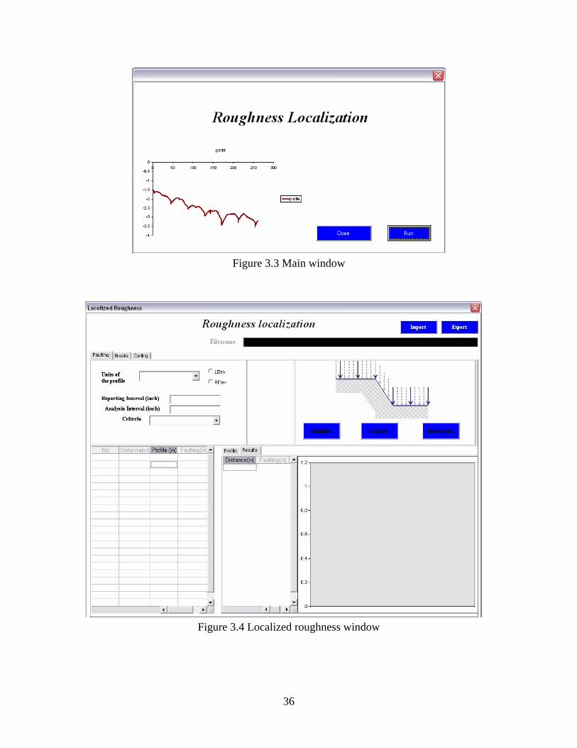
Figure 3.3 Main window

Figure 3.4 Localized roughness window

36

Table 3.1 summarizes the lines in an ERD file, and describes the parameters used in line #2 to describe the numerical data.

Table 3.1 Summary of records in an ERD file header Line No.

Description

1 ERDFILEV2.00 -- identifies file as having ERD format 2 NCHAN, NSAMP, NRECS, NBYTES, KEYNUM, STEP, KEYOPT -- use

commas to separate numbers: • NCHAN [integer] = Number of data channels. • NSAMP [integer] = Number of samples for each channel. • NRECS [integer] = Number of records of data. • NBYTES [integer] =Number of samples per record. • KEYNUM[integer] Indicates how the data are stored.

o 5, 15 = Formatted floating-point (text). The format must be specified using the FORMAT keyword.

For KEYNUM=5, the data are stored with all channels for the first sample together, then all channels for the second sample, etc. For KEYNUM=10,11, and 15, the data are stored with all samples for the first channel together, then all samples for the second channel, etc.

• Step [real] = sample interval (e.g., time step) • KeyOpt [integer] = auxiliary number used by some programs

Optional records. Each record be ins with an 8-character keyword, followed by information associated with that keyword.

g

Last Line

END -- indicates the end of the header

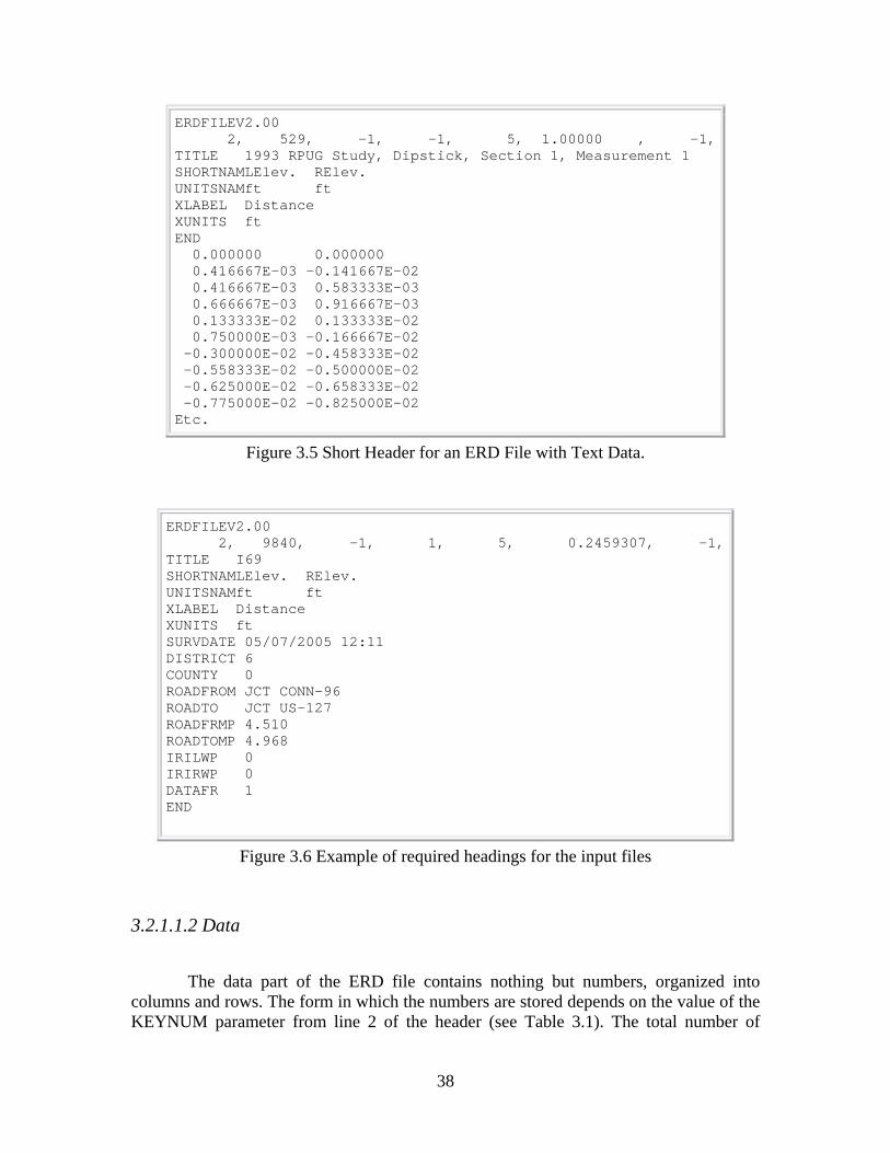
Figure 3.5 shows an example header which is fairly brief, consisting of the three required lines and four optional lines. (The optional lines are the ones beginning with the keywords TITLE, SHORTNAM, XLABEL, and XUNITS.)

Looking at the second line of the file shown in Figure 3.5, we see that the file

contains data for 2 channels, with 529 samples per channel, stored as 1 record, that the data storage format is type 5, that the interval between samples is 1.00, and that the status of the auxiliary numbers is -1. The header shown in Figure 3.5 includes names of the units for each channel, as identified with the keyword UNITSNAM. The name of units for the first channel, ft, has only two characters. Thus, it is followed by six spaces so that the name for the second channel, ft, begins in the correct column position.

Using the format of the ERD files that MDOT gave to the research team, the input

files (*.ERD) should include all the lines in the heading presented in figure 3.6. The software will work properly only if the input files follow the mentioned format.

37

ERDFILEV2.00 2, 529, -1, -1, 5, 1.00000 , -1,T

66667E-03 0.916667E-03 0.133333E-02 0.133333E-02 0.750000E-03 -0.166667E-02 . . . .Etc.

ITLE 1993 RPUG Study, Dipstick, Section 1, Measurement 1 SHORTNAMLElev. RElev. UNITSNAMft ft XLABEL Distance XUNITS ft END 0.000000 0.000000 0.416667E-03 -0.141667E-02 0.416667E-03 0.583333E-03 0.6

-0 300000E-02 -0.458333E-02 -0 558333E-02 -0.500000E-02 -0 625000E-02 -0.658333E-02 -0 775000E-02 -0.825000E-02

Figure 3.5 Short Header for an ERD File with Text Data.

ERDFILEV2.00 2, 9840, -1, 1, 5, 0.2459307, -1,TITLE I69 SHORTNAMLElev. RElev. UNITSNAMft ft XLABEL Distance XUNITS ft SURVDATE 05/07/2005 12:11 DISTRICT 6 COUNTY 0 ROADFROM JCT CONN-96 ROADTO JCT US-127 ROADFRMP 4.510 ROADTOMP 4.968 IRILWP 0 IRIRWP 0 DATAFR 1 END

Figure 3.6 Example of required headings for the input files 3.2.1.1.2 Data

The data part of the ERD file contains nothing but numbers, organized into columns and rows. The form in which the numbers are stored depends on the value of the KEYNUM parameter from line 2 of the header (see Table 3.1). The total number of

38

values that will appear in the data section is NCHAN x NSAMP. All of the numbers in e data portion are stored in the same format, and there can be no missing values.

th

3.2.1.2 Import window

The “Import” button in the localized roughness window opens a new screen asking the user to choose an ERD file name. Then, users should click on the “Open” button such that the application will extract all the relevant information about the site (Figure 3.7).

Figure 3.7 Import file window

3.2.1.3 Export window

The “Export” button in the localized roughness window opens a new screen asking the user to choose a file name and its path. Then, users could export to excel results using the “Save” button. Users should enter a file name followed by the extension “.xls” to export to excel file (Figure 3.8).

Figure 3.8 Export results window

3.2.2 Faulting Detection Window

Figure 3.9 shows the fault detection window. Users should choose between the right and left wheelpath from the raw profile. To do that, they should check the radio point that corresponds to the preferred wheelpath. Once checked, the application copies the raw profile to the column “Profile”.

39

40

Before analysis, users should specify the threshold (in inches) as well as the

reporting interval. If the worksheet is not empty, users should click on the “initialize” button. Then, they should click on the “analyze” button.

The output for the analysis will be shown on the “results” tab (Figure 3.9). The

application allows users to plot the raw profile on the “profile” tab (Figure 3.10). In order to get summary statistics as well as faulting distribution according to

their severity, the user should click on the “histogram” button (Figure 3.11). Users should enter a bin range to get fault distribution; otherwise, default values are used (corresponding to the severity level selected by the research team and defined in Table 2.1); i.e.,

• 0.25 low severity level • 0.5 Medium severity level • 0.75 high severity level

Figure 3.9 Fault detection results window

41

Figure 3.10 faulting detection window displaying the original profile

Figure 3.11 Fault results summary and distribution window

3.2.3 Breaks Detection Windo

irst, the mo ult detection module, users should specify the same inputs as for detecting faulting; i.e

ifferent, less than

3 feet, it is considered break; otherwise, th gives

as a res

w

Figure 3.12 shows the Breaks Detection window. Before detecting breaks, fdule detects any difference in elevation. Since, this part is the same as the fa

reporting interval and threshold. Second, if the sign of two successive faults is dthe Breaks detection module checks the distance between them: if the distance is

ere is no break. The 3 feet threshold can bechanged; however, the program would have to be modified to do that. This module

ult: • Starting Point of the break; • Width of the break; (length along the profile) • Fault magnitude at the stating point; and, • Fault magnitude at the end point

Figure 3.12 Breaks detection results window

42

43

.2.4 Curling Detection Window

Figure 3.13 shows the Curling Detection Module. First, the module cuts off the ng wavelengths (high frequency) and the short wavelengths (low frequency) to filter

ut the topography. A 4th order Butterworth band-pass filter is used. Second, the module splays the original and the filtered profile as shown in Figure 3.14. Third, the slope of e filtered profile will be computed and the local maximum and zero points of the slope nction will be detected. At the end, the zero point’s location and the difference in evation between zero and maximum point will be resumed. Users should specify only e reporting interval. Note that changing the reporting interval would not affect the sults.

3

loodithfuelthre

Figure 3.13 curling detection results window

Figure 3. 14 curling detection window displaying the original and the filtered profile

44

CON LU The is study was to develop a tool for detecting surface distresses that

re not ide om the video imaging using the longitudinal profiles of a pavement rface. As ated previo the di dis zed into two

ategories: • discontinuity – faults and breaks • stresses tha ear ea wit riod – cur g of PCC

vements The purpose of the work done in Phase I was to review and identify the most

ethods for detecting surface distresses. These m elet nalysis, t time-frequency analysis and he methods were valuated u ng simulated profile d iles T study was aimed at lecting a the mo cc e m e discrete elevation difference ethod was selected for fault and break detection. The discrete slope mlected fo urling detec . F tr ere eat the cted methods could be validated and finalized. The newly developed

lgorithms ere able to d t th gn e of 2 of .97 and s dard error (SE) of 0.25 mm. The n was als highly accurate (R2

ethods developed in this study can capture levant i mation abou ese hn feat easonable accuracy.

The final step was to develop a user-f puter software for detecting and quantif g new distre lting, breaks and curling). The

ftware sy em includes g

• input and o ut s m for handling the required data - selecti rofi ata anal- changing parameters (criteria/decision rules) for distr

methods - storing orti he cted

• means to display a co bi

A user manual is included in this repor llecte rom the field trials nd used in e evaluatio the ec ethod are presented in Appendix A. A copy f the softw e and the ra rofi f t ield ns are attached to this report.

his new t l could be u as a p entin ting PMS system. It r exam

r faulted cks..

C SION

ant

im of thifiable fra

su st usly, can date tresses can be summaric

Distresses that appear as profile Di t app rep tedly h some pe linpa

appropriate ma

ethods include: wavrete methods.join disc T

e si s an prof of LTPP sections. hese nd finalizing st a urat ethod. Thmse

ethod was ctions in Michigan so r c tion ield ials w held in different s

th selea w etec e ma itud faulting, breaks and curling with an R0=0.99). These results indicate that the m

tan localizatio o

re nfor t th roug ess ures with r

riendly, window-based comsystemso

yin sses (f:

aust the followin features

An utp yste

ng p le d for ysis ess identification

/rep ng t dete surface distresses

A m nation of profile data and results.

t. The data co d fa th n of sel ted mo ar w p les o he f trial sectio Tcan be used to enhance the PMS database; fo

oo sed com lem g module for the exple, by adjusti

isng the distress points

fo cra

45

R F EN

ttoh-Okin N. O. and M ah, Ch terizing pavement profile using wavelets analysis. Constructing Sm h h ex ents, ASTM STP 1433, 2003

yrum, C. A high speed profiler based slab curvature index for jointed concrete pavement curling and warping analysis. ertation. U iversity of Michigan. 2001

sen, R.O. (2005), ProVAL 2.7 User's Guide, ht www.roadp e.co

e Pont an . J. Scott, A yond a ghn o profile data., Road & T nsport Rese , v8 99 2-28

Fernando, E and Bertrand, C., Application of profile data to detect lTransportation Research Record, n 1813, 2002, 02-4050, p 55-61

rfanidis, . (1996), In ucti s l PR New Jersey

ayers, M. ERD Data-Processing So are R anual. V sion 2.00 Univeristy of Michigan Transportation Research Institute Report UMTRI-87-2, (1987) 109 p.

ayers and ramihas, Inter etatio f R d Rough -19, June 1996.

E ER CES

A e, ens S., aracoot ot m asphalt pavem

BPh.D Diss n

Chang ,G.K., Dick, J.C., and Rasmusm/. tp:// rofil

D d J , Be ro d rou ess – interpreting r adra arch , 19 , p1

ocalized roughness.,

all, Upper Saddle O S.J trod on to igna rocessing, Prentice-Hiver, .

S W. ftw eference M er

S Ka pr n o oa ness, UMTRI 96

46

APPENDIX A: FIELD TRIALS DATA

SITE 1

Distance Faulting (mm)

F In Left nt Average Explanation Other

eet ches Ce er Right

0 0 1.5 1 1.5 1.33Station 386+36

41 2 2.3 2.4 .60Joint 3.1 2

82 3 0.9 3.6 2.13Expansion Joint 1.9

123 4 0.6 1.2 .13Joint 1.6 1

164 2 0.5 1.4 1.7 .20Joint 1

191 7 Pothole with D = 6 in.

178 3 Pothole with D = 6 in.

205 6 1.1 2 2 1.70Joint

246 9 0.2 1.2 .03Joint 1.7 1

271 8 Pothole with D = 4 to 8 in.

287 11 2.3 4 .93Joint 5.5 3

301 4 6 in. brea t) 2 in. wide Crack k (3f

331 0 7 6.7 .07Joint 4.5 6

371 10 2.4 4.5 3.60Joint Negative patch 1ft before joint 3.9

413 7 5.3 5.3 9 .17Expansion Joint 4. 5

419 11 1.6 2.3 9 .27Crack 2. 2

435 5 Patch

454 7 6.5 5.9 7 .03Joint 5. 6

495 8 5 5.7 9 .20Joint

Shallow pothole (4 to 5 in. wide)

at 1 to 2 in. away from left

wheelpath 4. 5

536 8 5.3 5.4 9 .87Joint 3. 4

567 6 Station 392+00

577 9 3.8 4.5 9 .73Joint 2. 3

607 10 -0.4 0 -2.3 0.90Patch start -

614 1 -0.7 -0.3 1 h end 0. -0.30Patc

618 9 0.7 -1 2 t -3. -1.17Join

624 9 -0.7 5 -0.3 0.17Patch start 0. -

630 8 2.4 2.8 6 h end 1. 2.27Patc

659 6 6.2 5.2 5 t 5. 5.63Join

667 1 3+00 Station 39

700 6 6.3 5.3 5.77Joint 5.7

A-1

741 7 1.7 2.3 3 ansion Joint 2.33Exp

782 6 4.4 4.9 7 t 4. 4.67Join

823 6 3.8 3.6 3.57Joint 3.3

841 1 Pothole Figure A.1

848 3 -0.8 0.1 led Crack 0.2 -0.17Sea

864 7 3.5 1.7 9 2.37Joint 1.

883 11 Pothole Figure A.2

905 8 5.4 6.8 6.17Joint 6.3

946 8 5.4 5.8 9 t 4. 5.37Join

987 7 5.3 6.6 7 6. 6.20Joint

1028 8 6 1.8 9 .57Joint 2. 3

1069 8 5.1 4.3 3 4.90Expansion Joint 5.

1092 9 -0.4 0.5 led Crack 0.3 0.13Sea

1110 7 0.7 0.8 4 t 0. 0.63Join

1132 7 2.1 1 -0.7 0.43Sealed Crack Y crack with below (Figure A.3 ) -0.

1133 11 0 1.5 1.10Sealed Crack 1.8

1151 9 3.8 3.4 9 t 2. 3.37Join

1192 9 3.1 5.9 4.77Joint 5.3

1233 10 3.3 3.2 8 t 2. 3.10Join

1275 0 6.5 5.8 7 t 3. 5.33Join

1296 11 0.1 0.2 4 led Crack -0. -0.03Sea

1316 0 6.4 7.4 7.10Joint 7.5

1357 0 1.6 2.9 5 t 2. 2.33Join

1398 1 4.5 5.2 2 led Crack 7. 5.63Sea

1438 0 5.4 5.7 5.57Joint 5.6

1453 0 0.5 2.9 1 led Crack

4 in. by 1 ft. of spalling on right

wheelpath 3. 2.17Sea

1479 11 5.1 5.6 5 5.40Joint 5.

1520 0 3.8 5 2 t 5. 4.67Join

1562 0 0.8 2.3 8 t 2. 1.97Join

1603 1 7.9 8.2 8 7.97Joint 7.

1644 2 5.3 5.7 4 6. 5.80Joint

1685 1 3.5 4.4 3.83Joint 3.6

1726 1 3.5 4.2 6 ansion Joint 4. 4.10Exp

1736 1 4.9 4.9 4.87Sealed Crack 4.8

1769 2 1.7 3.6 3 t 4. 3.20Join

A-2

1808 1 3.1 5 4 t 5. 4.50Join

1849 4 4.8 5.1 5.07Joint

Right wheelpath joint width = 0.5

in. 5.3

1856 6 1.7 2.2 5 1. 1.80Crack

1896 0 4.7 5 5.6 5.10Joint

1931 7 3 2.6 4 3.33Joint 4.

1972 8 6.3 5.8 7 5.93Joint 5.

2013 11 4.4 4.2 9 .17Joint 3. 4

2026 3 -0.8 0 -0.1 0.30Sealed Crack -

2038 6 -0.6 -0.2 1 rack 0. -0.23Sealed C

2055 0 23.4 9.5 8 ansion Joint

Right wheelpath Joint width = 0.5

in. (Figure A.4 for Breaks) 4. 12.57Exp

2095 11 2.2 3.7 1 3.00Joint 3.

2137 1 3 3.3 3.13Joint 3.1

2158 8 -1 -0.2 Sealed Crack -0.7 -0.63

2171 4 Station 408+00

2178 5 4.4 6.3 5.30Joint 5.2

2219 6 1.5 2.5 2.20Joint 2.6

2267 1 1.6 2.6 2.17Joint Station 408+95 2.3

A-3

3 in. 1 in. 1 in.

Direction of Traffic

Figure A.2

1 in. 1 in.

Direc o Traffic tion f

2 in.

Figure A.1

Direction of raf T fic

Direction of Traffic

Figure A.4

Shoulder

18 in.

-8.5 mm -11.8 mm

Figure A.3

A-4

SITE 2

Distance Faulting (mm)

Feet Inches Left Center Right Comments 3 2 station 693+00

15 6 0.6 0.9 crack

44 1 joint

58 1 11 1 14.1 crack

69 10 -2.9 3 crack

85 9 joint

101 8 2.1 4.7 crack

126 6 joint

148 10 0.2 0.7 crack

167 8 joint

181 4 1.8 2.6 crack

209 3 joint

225 2 0.5 1.5 crack

251 0 joint

268 7 4.8 4.4 crack

276 9 -2.4 -1.8 crack

292 5 joint

307 1 2.4 7.2 1 crack

316 9 0.9 1.8 crack

334 0 joint

349 9 7.4 7.9 crack

363 1 -1.1 -1 0 crack

375 6 joint

399 10 3.3 4.5 crack

416 10 joint

431 1 0.2 2.3 d crack 1 seale

444 2 -1.1 - crack 0.5 sealed

458 7 joint

468 8 0.1 -0.5 d crack seale

477 1 -0.8 -0.6 d crack seale

487 1 3 ealed crack 0 1.6 .2 wide s

505 0 joint

A-5

516 7 0.9 2.7 sealed crack

527 0 0.1 -1.1 crack sealed

541 4 joint

554 4 -0.5 -0.5 crack

571 0 1.2 13 d crack seale

582 10 0.6 -0.7 joint

605 8 station 699+00

624 4 joint

635 6 -1.7 0 sealed crack

644 9 -0.5 1 ealed crack .5 partial s

650 8 7 5.9 crack

664 11 -0.3 0.2 joint

676 9 -0.2 -0.4 sealed crack

704 6 -1 0.5 d crack seale

770 0 joint

758 1 joint

778 3 0.4 0 crack .5 sealed

799 4 joint

812 8 6.5 1 crack 0.6 sealed

820 1 0.2 - crack 0.8 sealed

826 9 3.9 2.9 sealed crack

840 6 joint

858 2 3.5 4.5 sealed crack

867 1 -1.1 -0.3 d crack seale

882 1 joint

900 1 crack 0 -1.1 1 sealed

911 8 0.8 -1.1 d crack seale

923 1 -0.3 -1 joint

942 10 1.8 2.2 d crack seale

953 4 -0.5 -1 sealed crack

963 5 -0.5 -0.4 joint

988 8 2.8 4.8 wide sealed crack

1004 8 joint

1024 3 -1.4 -1 d crack seale

1045 4 joint

1063 1 -0.5 -0.3 sealed crack

A-6

1075 1 -1 01 sealed crack

1086 5 -0.3 0 joint

1128 1 joint

1167 5 -0.3 -0.3 sealed crack

1169 4 joint

1210 0 0.5 1.2 joint

1251 5 0.4 0 joint

1274 1 -1 1 0.7 crack

1293 6 joint

1306 8 4.5 6.6 wide sealed crack

1334 8 1.8 0.7 joint

1343 5 0.4 0 sealed crack

1374 7 1.9 1.4 joint

1415 9 joint

1456 8 joint

1497 7 joint

1538 4 joint

1579 2 joint

1620 2 joint

1661 3 joint

1688 1 -1.2 0.2 d crack 1 seale

1701 6 -0.1 0.3 joint

1732 1 0.3 crack 0 0 sealed

1742 4 joint

1756 5 -0.8 1 sealed crack

1783 3 joint

1824 1 joint

1843 7 0.2 -0.5 d crack seale

1865 4 joint

1906 2 joint

1947 2 joint

1988 1 joint

2029 1 joint

2069 11 0.9 0.6 joint

2085 4 1.6 2.3 sealed crack

2096 11 5.3 4.6 sealed crack

A-7

2101 2 -0.1 2 sealed crack

2110 8 -0.3 0.4 joint

2151 3 0 -0.3 joint

2192 5 0.1 -0.6 joint

2233 0 joint

2274 0 joint

2315 0 joint

2356 0 joint

2397 0 joint

2438 0 joint

2479 0 joint

2506 3 0 -0.9 d crack seale

2520 0 joint

2561 0 joint

2572 8 -0.2 l sealed crack partia

2602 0 joint

2616 9 -0.2 -0.9 d crack seale

2629 1 3 ealed crack 1 4.4 .8 wide s

2643 0 joint

2684 0 joint

2720 1 station 720+00

2725 8 joint

24 4 error

A-8

SITE 3

tance Dis Faulting (mm)

Feet Inches Left Center Comments Right 0 0 station 773+00 (core)

22 8 joint

32 9 4.6 8 ck cra

63 5 joint

87 4 -0.5 0 crack

104 4 joint

145 7 joint

186 4 joint

199 4 0.7 4.1 crack

227 2 joint

234 7 1.4 5.3 crack

258 8 1.6 4.3 crack

267 8 joint

300 6 station 776+00

309 4 joint

350 2 joint

362 4 1 3.3 crack

391 2 joint

432 3 joint

456 9 4 9.5 crack

465 0 1.6 1.6 crack

473 1 joint

488 2 0.6 1 crack

500 11 station 778+00

503 3 5.8 6 crack

514 1 joint

526 6 4.4 6.8 crack

554 11 joint

596 4 joint

636 11 joint

649 3 5.8 7 crack

A-9

656 4 3.2 3.3 crack

662 5 -1.6 crack

6 5 8 crack 65

672 2 diagonal crac -2.4 k

678 2 joint

701 4 station 780+00

719 1 joint

747 9 mid-slab (8inch) deep>1inch

759 10 0.5 0.3 joint

790 1 -0 0.4 2 crack

800 10 joint + station 781+00

814 1 3.7 7.6 wide crack

822 1 -0 0.8 0.6 crack

841 11 joint

854 6 5.6 8 rack .3 c

882 10 joint

897 9 2.5 6 crack

923 10 joint

933 3 2.3 5.9 crack

945 0 8.3 9.6 crack

955 7 0.3 1.8 crack

964 9 joint

1001 7 station 783+00

1005 10 joint

1046 10 joint

1063 8 4.3 8 crack

1087 10 joint

1100 2 4.1 8.9 crack

1128 10 joint

1137 10 -0.3 0.7 crack

1143 7 3.5 6.3 crack

1153 6 -0.4 4.4 partial crack

1158 1 -0 -1 1.8 crack

1169 2 joint

1183 5 3.4 6.4 crack

1196 5 3.4 3.5 space wide crack

A-10

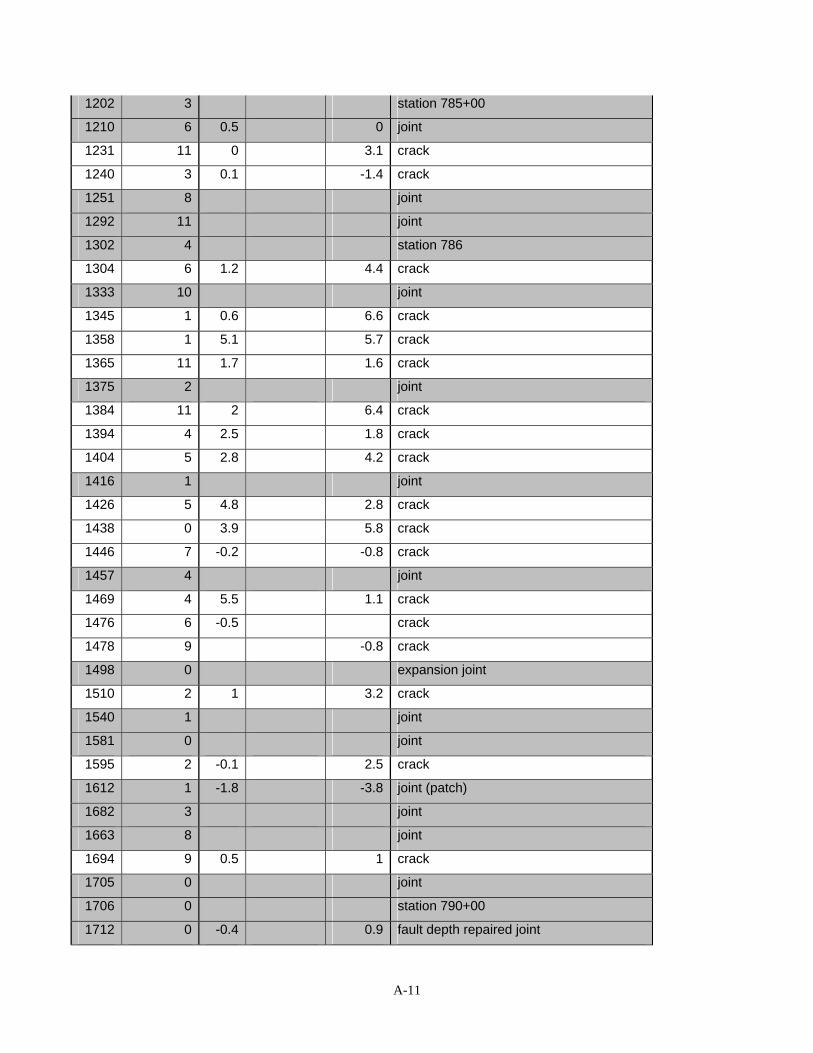
1202 3 station 785+00

1210 6 0.5 0 joint

1231 11 0 3.1 crack

1240 3 0.1 - 1.4 crack

1251 8 joint

1292 11 joint

1302 4 station 786

1304 6 1.2 4.4 crack

1333 10 joint

1345 1 0.6 6.6 crack

1358 1 5.1 5.7 crack

1365 1 1 1.7 1.6 crack

1375 2 joint

1384 11 2 6.4 crack

1394 4 2.5 1.8 crack

1404 5 2.8 4.2 crack

1416 1 joint

1426 5 4.8 2.8 crack

1438 0 3.9 5.8 crack

1446 7 -0.2 - 0.8 crack

1457 4 joint

1469 4 5.5 1.1 crack

1476 6 - 0.5 crack

1478 9 - 0.8 crack

1498 0 expansion joint

1510 2 1 3.2 crack

1540 1 joint

1581 0 joint

1595 2 -0.1 2.5 crack

1612 1 -1.8 -3.8 joint (patch)

1682 3 joint

1663 8 joint

1694 9 0.5 1 crack

1705 0 joint

1706 0 station 790+00

1712 0 -0.4 0.9 fault depth repaired joint

A-11

1732 1 -1.7 4 end of previous joint

1746 1 1 2.5 joint

1787 6 joint

1828 6 joint

1869 6 joint

1910 7 joint

1951 6 joint

1993 5 joint

2034 6 1.6 0.6 joint

2053 8 5.2 6.3 crack

2063 5 -0.4 0.3 spoiled crack

2076 3 joint

2094 6 0 0.8 crack

2116 8 joint

2158 2 joint

2199 3 -0.3 0.8 joint

2240 5 joint

2255 6 -0.2 0 crack

2281 8 joint

2297 8 3.1 3.7 crack

2323 0 joint

2364 3 joint

2379 0 1 2.1 crack

2405 4 joint

2408 8 station 797+00

2434 9 0 1.7 crack

2446 7 joint

2459 4 -0.5 - 0.7 crack

2488 1 joint

2504 4 1.5 3.3 crack

2512 3 5.1 2 .2 crack

2520 3 -1.5 -1.4 crack

2529 3 joint

2541 7 5.6 6.5 crack

2550 1 1.3 1.2 crack

2570 11 0.3 1 joint

A-12

2612 1 joint

2631 1 4.3 6 crack

2640 1 0.2 -0.3 crack

2653 3 joint

2694 7 joint

2712 1 (core) station (800+00)

12 0 error

A-13

SITE 4

tance lting (mm) Dis Fau

Feet Inches L Rig Comments eft Center ht 0 0 station 130+00

0 6 10 9.1 joint

57 1 1.9 1 repaired joint (patch)

110 4 2 4.3 t (patch) repaired join

166 4 0.7 2.5 ck (10'' wide) spoiled cra

216 4 8.4 7.9 joint

266 1 5.4 4.9 wide crack

287 8 9.4 8.3 joint

323 1 0.5 0.4 0'' wide) spoiled crack (1

358 9 6.6 15.3 spoiled joint (4'' wide)

9

399 4 3.5 7 patch joint

430 4 8.8 6.2 joint

445 7 2.9 5 crack (3'' wide) spoiled

501 6 station 135+00

501 11 9.8 7.8 joint

523 8 -0.7 2.3 crack

573 7 6 5.2 joint

644 11 3.9 6.4 spoiled joint

665 7 4.5 6.5 repaired joint (patch)

716 4 8.1 7.1 joint

738 5 3.7 3.5 repaired joint (patch)

787 6 7.3 6.6 joint

837 2 4.3 4.9 spoiled crack

859 2 6.6 7.2 joint

930 10 4.1 5.7 joint

954 6 4.9 5.3 rack wide c

1003 1 3.2 3.3 station 140+00

1045 5 1.6 1.2 patch joint

1073 8 7.2 5.4 joint

1106 9 3.7 2.8 crack

1119 8 3.2 4.3 crack

A-14

1145 6 10 8.5 joint

1166 1 1.1 5.5 repaired joint (patch)

1194 5 4.5 4.8 repaired joint (patch)

1217 1 10.8 7.7 joint

1235 11 start patch

1242 6 patch end of

1288 4 6.9 5.6 joint

1337 3 start patch

1343 10 -0.4 0.9 end of patch (repaired joint)

1381 9 start patch

1400 0 3.2 5.5 end patch (repaired patch)

1431 8 5.6 5.5 joint

1448 8 6.1 5 crack

1467 5 5.4 8.5 crack

1483 6 start patch

1490 2 end patch (repaired patch)

1520 1 6.7 5.7 crack 0 wide

1546 6 atch start p

1553 0 end patch

1575 0 8.2 8.4 joint

1593 5 0.3 ck 0.8 cra

1611 10 start patch

1646 10 3.3 2 end patch (repaired joint)

1666 4 2.8 3.7 crack

1677 4 8 6.1 crack

1699 3 1.8 4.3 crack

1706 8 station147+00

1718 6 8 7.8 joint

1737 1 8 9.1 rack 1 wide c

1750 9 4.5 3.5 crack

1790 0 8.1 6.6 joint

1861 6 5.5 6.6 joint

1877 0 crack

1894 8 -10.8 -5.9 start patch

1920 4 atch end p

1933 0 8.6 6.3 joint

A-15

1953 6 atch start p

1960 1 end patch

1972 5 art patch st

1986 9 nd patch + start patch e

1995 10 nd patch e

2004 8 9.7 9 joint

2019 7 tart patch s

2039 9 end

2053 4 start patch

2059 10 end

2075 9 13.8 10.7 joint

2092 1 start patch

2098 6 end

2118 3 start patch

2124 10 -0.6 0.3 end patch (repaired joint)

2147 4 8.9 6.7 joint

2167 7 start patch

2173 11 end

2189 0 crack

2195 10 crack

2208 3 station 152+00

2218 7 13.8 9.1 joint

2234 0 start patch

2240 11 end

2265 11 4.6 1.1 start patch

2272 6 end

2290 4 7.5 6.5 joint

2310 3 6.9 7.6 crack

2324 11 start patch

2344 5 end patch

2361 7 6.3 5 joint

2403 1 -2.6 -4.8 start patch

2420 11 6 3.1 end

2461 10 start patch

2468 6 0.9 1.6 end

2504 9 5.1 3.4 joint

A-16

2509 8 station 155+00

2532 2 start patch

2538 8 4.3 3.4 end

2557 3 start patch

2563 9 1.8 4.8 end patch

2576 4 12 10.9 joint

2627 6 start patch

2634 4 4.8 5.8 end

2647 8 9.1 7.1 joint

2667 1 start patch

2673 7 6 6.3 end patch

2682 3 start patch

2688 11 1.5 4.1 end

2697 6 start patch

2704 0 end

2710 7 station 157+00

2737 11 -0.8 -2.2 start patch

2752 11 end

2771 5 start patch

2778 0 -1.7 1.8 end

2791 0 8.1 10.9 joint

2858 11 start patch

2865 4 3 4.3 end

2892 1 4.6 5.3 crack

2933 8 9 10.5 joint

2967 3 crack

2975 6 start patch

2982 0 5.4 4.2 end

3005 1 5.7 4.5 joint

3011 6 station 160+00

3036 7 4.7 3.8 crack

3057 7 start patch

3064 1 end

3076 7 8 8 joint

3111 5 crack

3127 4 5.8 3.9 crack

A-17

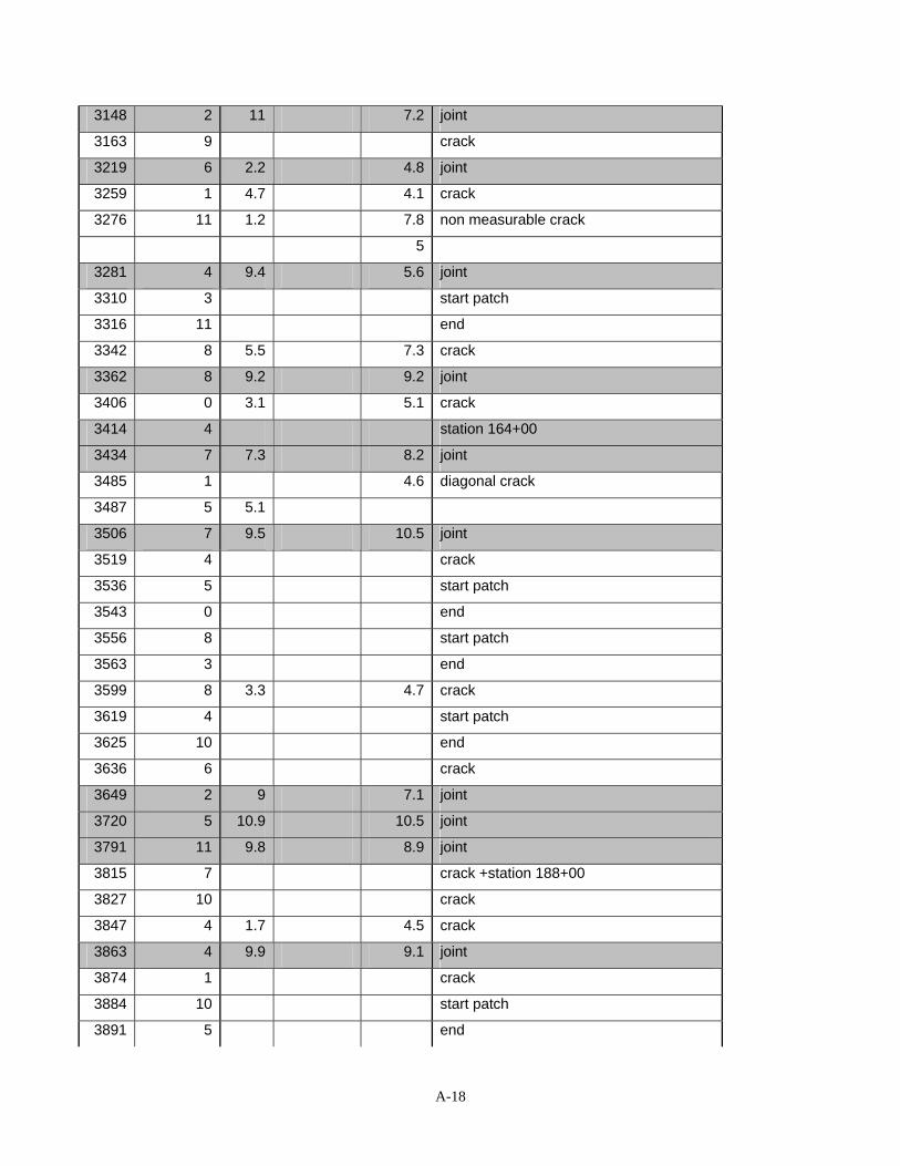
3148 2 11 7.2 joint

3163 9 crack

3219 6 2.2 4.8 joint

3259 1 4.7 4.1 crack

3276 11 2 7.8 non measurable crack 1.

5

3281 4 9.4 5.6 joint

3310 start pat3 ch

3316 e11 nd

3342 8 5.5 7 crack .3

3362 8 9.2 9.2 joint

3406 0 5.1 crack 3.1

3414 4 station 164+00

3434 7 7.3 8.2 joint

3485 1 4.6 diagonal crack

3487 5 5.1

3506 7 9.5 10.5 joint

3519 4 crack

3536 5 start patch

3543 0 end

3556 8 start patch

3563 3 end

3599 8 3 4.7 crack 3.

3619 4 start patch

3625 10 end

3636 6 crack

3649 2 9 7.1 joint

3720 5 10.9 10.5 joint

3791 11 9.8 8.9 joint

3815 7 crack +station 188 00 +

3827 10 crack

3847 4 1.7 4.5 crack

3863 4 9.9 9.1 joint

3874 1 crack

38 start patch 84 10

3891 5 end

A-18

3915 9 2.1 2.1 crack +station 169+00

3948 2 start patch

3954 9 end

3966 5 tch start pa

3972 11 end

3986 11 6.2 4.2 crack

4021 5 start patch

4040 6 end

4077 7 7.5 8.6 joint

4116 11 station 171+00

4120 7 2.3 5.2 crack

4142 0 crack

4149 1 9.7 9.7 joint

4164 11 crack

4173 6 0.6 1.3 spoiled crack

4192 4 start patch

4203 6 end

4220 10 3.8 4.7 joint

4241 0 crack

4248 2 2.4 diagonal crack

4249 2 2.4

4266 1 crack

4276 1 crack

4292 2 7 7.4 joint

4308 6 4.5 5.7 crack

4317 11 station 173+00

4326 11 5.2 6.9 crack

4363 10 10.5 10.3 joint

4375 4 crack

4389 5 8 8.8 crack

4400 0 7.7 8 crack

4418 7 station 174+00

4435 4 8 7.6 joint

4450 4 2.3 -1.7 start patch

4470 7 6 5.6 end

4490 0 7.5 7.8 crack

A-19

4506 10 9.2 10.3 joint

4524 11 6.8 25.8 spoiled crack

18.5

2 1 error

A-20

APPENDIX B: REPEATED MEASUREMENTS

B-1

SITE 2

Repeatability test

Distance Faulting (mm)

Feet Inches Left Center Right Comments 650 8 7 5.9 crack

Direction

traffic transversal

repeated

measure

6 5.1 5.9

6 5.9 5.5

5.8 6.3 5.7

5.9 6.3 5.8

5.1 5.5 5.8

5.5

5.7

5.6

5.7

5.7

5.5

5.7

5.8

5.8

5.6

interval

(inch) 3 6

average 5.76 5.82 5.686667

standard

error 0.1144 0.2176 0.014489

B-2

SITE 3

Repeatability test (1)

Distance Faulting (mm)

Feet Inches Left Center Right Comments 2541 7 5.6 6.5 crack

Direction

traffic transversal

repeated

measure

7.7 6.8 7.1

7.1 7 7.2

6.8 6.8 7.1

7.1 7.1 7.1

6.9 6.5 7

7.5 7

7.4 7.1

7

7.2

6.9

6.9

7

7.2

6.8

7.1

interval

(inch) 4 6

average 7.12 7.014286 7.046667

standard

error 0.0976 0.106939 0.013156

B-3

Repeatability test (2)

Distance Faulting (mm)

Feet Inches Left Center Right Comments 1476 6 -0.5 crack

Direction

traffic transversal

repeated

measure

-0.4 -0.3 -0.5

-0.4 -0.5 -0.5

-0.2 -0.2 -0.5

-0.7 -0.2 -0.6

-0.6 -0.7 -0.5

-0.7

-0.7

-0.5

-0.5

-0.7

-0.7

-0.6

-0.8

-0.3

-0.5

interval

(inch) 4 6

average -0.46 -0.38 -0.57333

standard

error 0.0304 0.0376 0.015289