Contemporary MathematicsVolume 319, 2003

MEASURE THEORY AND INTEGRATION ON THELEVI-CIVITA FIELD

KHODR SHAMSEDDINE AND MARTIN BERZ

ABSTRACT. It is well known that the disconnectedness of a non-Archimedeantotally ordered field in the order topology makes integration more difficultthan in the real case. In this paper, we present a remedy to that difficulty andstudy measure theory and integration on the Levi-Civita field. After reviewingbasic elements of calculus on the field, we introduce a measure that proves tobe a natural generalization of the Lebesgue measure on the field of the realnumbers and have similar properties. Then we introduce a family of simplefunctions from which we obtain a larger family of measurable functions andderive a simple characterization of such functions. We study the properties ofmeasurable functions, we show how to integrate them over measurable sets of'R., and we show that the resulting integral satisfies similar properties to thoseof the Lebesgue integral of real calculus.

1. INTRODUCTION

Measure theory and integration on the Levi-Civita field n [5, 6] are presented.We start with a review of some basic and useful terminology and refer the readerto [1, 10, 2, 11] for a more detailed study of the Levi-Civita field. For a generaloverview of the algebraic properties of formal power series fields in general, werefer to the comprehensive overview by Ribenboim [9], and for an overview of therelated valuation theory the book by Krull [3]. A thorough and complete treatmentof ordered structures can also be found in [8].

Definition 1.1 (The set n). We define n = {f : Q -+ R : {XE Q : f(x) # O} isleft-finite}. So the elements of n are those real valued functions on Q that are

1991 Mathematics Subject Classification. 11S80, 12J25, 26E30, 46S10.Key words and phmses. Levi-Civita field, non-Archimedean calculus, measurable sets, mea-

surable functions, integration.This research was supported by an Alfred P. Sloan fellowship and by the United States De-

partment of Energy, Grant # DE-FG02-95ER40931. @ 2003 American Mathematical Society

369

I

..

310 KHODR SHAMSEDDINE AND MARTIN BERZ

non-zero only on a left-finite set, i.e. below every rational number q there are onlyfinitely many points where the given functions do not vanish.

We denote elements of n by x, y, etc. and identify their values at q E Q withbrackets like x[q]. This avoids confusion when we consider functions on n. For thefurther discussion, it is convenient to introduce the following terminology.

Definition 1.2 (supp, >., "'"', ~, =r)' For x E n, we denote {q E Q : x[q] ~ O} bysupp(x) and call it the support of Xj and we define >.(x) = min(supp(x)) for x ~ 0(which exists because of left-finiteness), and >'(0) = +00.

Comparing two elements x and y in n, we say x "'"' y if >.(x) = >.(y), x ~ y if>.(x) = >.(y) and x[>.(x)] = y[>.(y)], and x =r Y if x[q] = y[q] for all q ~ T.

At this point, these definitions may feel somewhat arbitrarYj but after havingintroduced the concept of ordering on n, we will see that>. describes "ordersof infinite largeness or smallness", the relation "~" corresponds to agreement upto infinitely small relative error, while ""'"',, corresponds to agreement of order of

magnitude.

Definition 1.3 (Addition and Multiplication on n). We define addition on ncomponentwise: (x + y)[q] = x[q] +y[q]. Multiplication is defined as follows: Forq E Q, we set (x. y)[q] = Eqz+q,,=qx[qx]" y[qy].

Since elements ofn have left-finite supports, only finitely many terms contributeto the sum in the definition of multiplication. Thus, .is a well defined operationon n. It turns out that the operations + and .make (n,+,.) into a field, in whichwe can isomorphically embed JR as a subfield via the map n : JR -t n defined by

{ X ifq=O(1.1) n(x)[q] = 0 th ..0 erwIse

Definition 1.4 (Ordering in n). Let x, y be distinct elements of n. We say x > yif (x -y)[>.(x -y)] > O. Furthermore, we say x < y if y > x. i

With thi~ defini~ion of t~e order r~lation~ n is a totally ord~r~ field. Moreover,

the embedding n ill (1.1) IS compatIble wIth the order. BesIdt the usual order

relations, some other notations are also convenient. I,i

Definition 1.5. «<,» ) Let a, b be non-negative. We say a isl infinitely smallerthan b (and write a « b) if n .a < b for all natural nj we say a }S infinitely largerthan b (and write a » b) if b «a. If a « 1, we say a is infinitel(y smallj if 1 « a,we say a is infinitely large. Non-negative numbers that are neither infinitely smallnor infinitely large are also called finite.

Definition 1.6 (The Number d). Let d be the element of n given by d[l] = 1 andd[q] = 0 for q ~ 1.

It is easy to check that 0 < d «1. It follows that, altogether, t~e Levi-Civita n isa totally ordered non-Archimedean field extension of the real numbers. It is shown[1] that this field is totally disconnected in the natural topolo~ induced by theorder. Because of this disconnectedness, which translates into the existence of anenormous number of "holes" between the different orders, supre~ and infima evenof bounded sets do not always exist. Moreover, there are nonconstant differentiablefunctions with vanishing derivatives everywhere on n; consequently, for a given

.

MEASURE THEORY ANI) INTEGRATION ON THE LEVI-CIVITA FIELD 371

function there could ex.ist multiple anti-derivatives. Thus, trying to extend theRiemann integral or the Lebesgue integral from JR to R is not all straightforward.

In this paper, we successfully circumvent the difficulties mentioned above anddefine a measure on the Levi-Civita field R that we prove is a natural generalizationof the Lebesgue measure on JR and has similar properties. Namely, we show thatany subset of a measurable set of measure 0 is itself measurable and has measureo. We also show that any countable unions of measurable sets whose measuresform a null sequence is measurable and the measure of the union is less than orequal to the sum of the measures of the original sets; moreover, the measure ofthe union is equal to the sum of the measures of the original sets if the latter aremutually disjoint. Then we show that any finite intersection of measurable sets isalso measurable and that the sum of the measures of two measurable sets is equalto the sum of the measures of ttleir union and intersection.

We introduce the concept ~f measurable functions on measurable sets of Rthrough a smaller family of simple functions, we derive a simple characterization ofsuch functions and we show that they form an algebra. Then we show that a mea-surable function is differentiable almost everywhere and that a function measurableon two measurable subsets of R is also measurable on their union and intersection.

We define the integral of a measurable function lover a measurable set A andshow that the integral satisfies similar properties to those of the Lebesgue andRiemann integrals on JR. In particular, we prove the linearity property of theintegral and that if IllS M on A then If A II S Mm(A), where m(A) is themeasure of A. We also show that the sum of the integrals of a measurable functionover two measllIable sets is equal to the sum of its integrals over the union and theintersection of the two sets. Finally, we show that if (J n) is a sequence of measurablefunctions on a measurable set A that converges uniformly on A, then the integralsof In over A form a converging sequence in R. Moreover, if the uniform limit Iof the functions In is itself measurable on A, then its integral fA I is equal to thelimit of fA In.

2. MEASURABLE SETS

Before we define a measure on R, we introduce the following notations whichwill be adopted throughout this paper: I (a, b) will be used to denote anyone of theintervals [a, b), (a, b), [a, b) or (a, b), unless we explicitly specify a particular choiceof one of the four intervals. Also, to denote the length of a given interval I, we willuse the notation l(I).

Definition 2.1. Let A c R be given. Then we say that A is measurable if forevery f > 0 in R, there ex.ist a sequence of mutually disjoint intervals (In) anda sequence of mutually disjoint intervals (In) such that Ur:'=1In C A c U~1Jn,E'::=1l(In) and E'::=1l(Jn) converge in R, and E'::=1l(Jn) -~'::=1l(In) Sf.

Given a measurable set A, then for every kEN, we can select a sequence ofmutually disjoint intervals (I~) !and a sequence of mutually disjoint intervals (J~)such that E'::=1l (I~) and E'::~1l (J~) converge in R for all k,

00 00

Ur:'=1I~ C U~=1I~+1 C ACU~+1J~+1 c U~=1J~ and ~ l (J~)' -~ l (I~) S dkn=1 n=1

, .

372 KHODR SHAMSEDDINE AND MARTIN BERZ

for all kEN. Since 'R is Cauchy-complete in the order topology, it follows thatlimk--+(X) E'::=l l (I~) and limk--+oo E'::=ll (J~) both exist and they are equal.. Wecall the common value of the limits the measure of A and we denote it by m(A).Thus,

(X) (X)

(2.1) m(A) = Jim L l (I~) = Jim L l (J~).k--+(X) k--+(X)n=l n=l

Moreover, since the sequence (E':=ll (I~)) kEN is nondecreasing and since the se-quence (E'::=ll (J~))kEN is nonincreasing,we have that

(X) (X)

(2.2) L l (I~) :$ m(A) :$L l (J~) for all kEN.n=l n=l

Contrary to the real case, sup {E~ll(In) : In's are mutually disjoint intervalsand U':>=lIn C A} and inf{E~ll(Jn): A c U~lJn} need not exist for a givenset A c 'R. However, as we will show in Proposition 2.2, if A is measurable thenboth the supremum and infimum exist and they are equal to m(A). This showsthat the definition of measurable sets in Definition 2.1 is a natural generalizationof the Lebesgue measure of real analysis that corrects for the lack of suprema andinfima in non-Archimedean totally ordered fields.

Proposition 2.2. Let A c 'R be measurable. Then

m(A)

= inf {fl(Jn): In is an intervalVn,ACUC;>=lJn and fl(Jn) converyes}n=l n=l

= sup{f l(In) : In's are mutually disjoint, UC;>=l In cA, f l(In) converyes}.n=l n=l

Proof. First we show that the infimum exists and is equal to m(A). Using Equation(2.1) and' Equation (2.2), it remains to show that if (In) is a sequence of intervalssuch that E'::=ll(Jn) converges and A c U':>=lJn then m(A):$ E'::=ll(Jn). As-sume not, then there exists a sequence of intervals (J~) such that E~ll (~)converges, A c U':>=lJ~, but m(A) > E'::=ll (J~). Let kEN be such that

dk < m(A) -E'::=ll (J~)2

and let (I~) and (J~) be as in the discussion leading to Equation (2.1) and Equation(2.2). Then U':>~1.I~ C A c U':>=l J~ and E'::=ll (J~) -E'::=ll (I~) :$ dk. SinceU':>=l I~ c Ac U':>=l ~ and since the intervals I~ are mutually disjoint, we obtainthat

(X) (X)

(2.3) L l (J~) ?: L l (I~) .n=l n=l

On the other hand, it follows from Equation (2.2) that(X) (X) (X)

m(A) -L l (I~):$ L l (J~) -L l (I~) :$ dk.n=l n=l n=l

--

MEASURE THEORY AND INTEGRATION ON THE LEVI-CIVITA FIELD 373

Thus,

~l(J~) -~l(I~) = (~l(~) -m(A)) + (m(A)-~l(I~))

:$ (~l(~) -m(A)) ~dk

< ( f l(J~) -m(A) ) +m(~)-:~:=l ((~)n=l

= E:=ll (~) -?fiCA)2

< 0,which contradicts Equation (2.3).

Similarly, we show that sup {E:=ll(In) : In is an interval for each n, In's aremutually disjoint, Uc:'=l In c A and E:=ll(In) converges} exists and is equal tom(A). D

It follows directly from Definition 2.1 and Proposition 2.2 that m(A) ?: 0 for anymeasurable set A c 'R. and that any interval I(a, b) is measurable with measurem(I(a, b)) = b- a. It also follows that if A is a countable union of mutually disjointintervals (In(an,bn))su~hthat E:=l(bn-an) converges then A is measurable withm(A) = E~l(bn -an). Moreover, if Bc A c 'R. and if A and B are measurable,then m(B) :$ m(A).

Proposition 2.3. Let A c 'R. be measurable with m(A) = 0 and let B C A. ThenB is measurable and m(B) = O.

Proof. First we show that B is measurable. Let f > 0 in 'R. be given. By Proposi-tion 2.2, there exists a sequence of mutually disjoint intervals (In) such that A CUc:'=lJn, E~ll(Jn) converges in 'R., and E~ll(Jn) :$ f. For each n E N, let In =0. Then Uc:'=lIn C B c Uc:'=iJn and E~ll(Jn) -E:=ll.(In) = E:=ll(Jn) :$ f.Hence B is measurable. Since B C A, we obtain that 0 :$ m(B) :$ m(A) ~ O.Thus, m(B) = O. ,".'0

Proposition 2.4. Let A C 'R. be countable. Then A is measurable and m(A)~ o.,

Proof. Since A is countable, we may write A = {an : n EN}. Now let f > 0 begiven in 'R.; for each n E N, let ~ = (an -~f, an + ~f) and In = J~ \ U:;;;! J?Then Uc:'=l In is a countable union of mutually disjoint intervals which we canwrite as K1, K2,. .., where Kl = Jl = Jp, K2 and K3 are the two mutually disjointintervals in J2 = Jg \ Jp, and so on. Since U~l Ki = Uc:'=l In = Uc:'=l J~, we obtainthat A c U~lKi. Also, since ~mn--+co l (J~) = limn--+co 2~f = 0, it follows thatlimi--+co l(Ki) =0. Hence E:ll(Ki) converges in'R. {II] and

co co co 2d}:l(!fi):$}:l (~) = }:2~f = r=df < £.i=l n=l ~=l

Now for all i E N, let Ii = 0. Then U~lIi C A C U~lKi and E:ll(Ki) -E:ll(Ii) = E:ll(Ki) < f. Thus, A is measurable. Moreover, by Proposition2.2, we have that m(A) :$ E:ll(Ki) <f. This is true for all f > 0 in 'R.; andhence m(A) = o. D

374 KHODR SHAMSEDDINE AND MARTIN BERZ

The converse of Proposition 2.4 is not necessarily true, that is if A is measurableand if m(A) = 0 then A need not be countable, as the following example shows.

Example 2.5 (Cantor-like Set). A Cantor-like set On is constructed in the sameway as the standard real Cantor set OJ but instead of deleting the middle third,we delete the middle (1 -2d)th of each of the closed subintervals of [0,1] at eachstep of the construction. So first, we delete the interval (d, 1 -d) from the intervalFo = [0,1.] and let FI denote the remaining closed set consisting of the two closedintervals [0, d] and [1 -d, 1] of length d each. Then we delete the open intervals(~, d -~) and (1- d + ~, 1 -~), and let F2 denote the remaining closed setwhich consists of four closed intervals [O,~], [d -~, d], [1 -d, 1 -d + d2] and[1 -~ , 1] of length ~ each. Then we delete the middle (1 -2d)th from each ofthese four intervals, getting a new closed set F3, consisting of eight closed intervalsof length d3 each, and so on. Continuing this process indefinitely (as we do in theconstruction of the real Cantor set 0), we get a sequence of closed sets F n suchthat Fn C Fn-l for all n E N. The intersection On = n':;'=oFn will be called theCantor-like set.

Clearly, On is closed and uncountable since there is a one-to-one correspondencebetween 0 and On. We leave it as an exercise for the reader to show that while 0 isnot measurable in the context of the measure defined here on R, On is measurableand m (On) = o.

Proposition 2.6. For each kEN, let Ak C R be measurable such that (m(Ak))forms a null sequence. Then U~=l Ak is measurable and

00

m (U~=l Ak) ~ L m (Ak) .k=l

Moreover, if the sets (Ak)~=l are mutually disjoint, then00

m(U~=IAk) = Lm(Ak).k=l

Proof. First we note that, since limk-+oo m(Ak) = 0, the sum L~l m(Ak) con-verges [11]. Now let t: > 0 in R be given. Then for each kEN there e.~s~ asequence of mutually disjoint intervals (I~) and a sequence of mutually dlSJomtintervals (J~) such that E"::=ll (I~) and E"::=ll (J~) converge in R, U':;'=II~ CAk C U':;'=IJ~, and E"::=ll(J~) -E"::=ll(I~) ~ dkt:. Since limk-+oom(Ak) = 0and since E"::=ll (I~) ~ E"::=ll (J~) ~ m(Ak) + dkt:, we obtain that

00 00

lim ~ l (I~) = lim L l (J~) = o.k-+oo L.., k-+oo

In=l n=

Thus, we can write U~=l U':;'=l J~ and U~=l U':;'=l I~ as unions of mutually ~isjointintervals, say U~IJi and U~IIi, such that U~IIi C U~=IAk C U~IJi, Ei=ll(Ji)and E:Il(Ii) converge and

~l(Ji) -~l(Ii) ~ ~ (~l (J~) -~l (I~))

00 d~ }:dkt:= ~t: <t:o

k=l

MEASURE THEORY AND INTEGRATION ON THE LEVI-CIVITA FIELD 375

This shows that U~=1 Ak is measurable.S.00 A 00 J 00 00 Jk bt " h tmce Uk=1 k C Ui=1 i = Uk=1 Un=1 n' we 0 am t a

00 00

m (U~=1 Ak) $ m (U~=l U';'=1 J~) $ ~ ~ 1 (J~)k=1n=1

00 00

$ L (m(Ak) +dkf.) < Lm(Ak) + f..k=1 k=1

This is true for all f. > 0 in Rj and hence00

(2.4) m(U~1Ak) $ Lm(Ak).k=1

Now assume that the measurable sets Ak are mutually disjoint, and let f. > 0in R be given. Then there exists KEN such that Ek>K mlAk) < £/2. Alsoby Proposition 2.2, since U~=1 Ak is measurable, there exists a sequence of mutu-ally disjoint intervals (In) such that U~=1 Ak C U~1 J~, E":=1l(J~) converges,and E":=1l( In) < m (U~=1Ak) + f./2. Since Ak C U~1 Ai C U';'=1 In for allk E {I, 2,..., K}, and since A1, A2'...' AK are mutually disjoint, it follows thatfor each k E {I, 2,. .., K}, there exists a sequence of mutually disjoint inter~vals (J~) such that E":=1l (J~) converges in R, Ak C U~lJ~ C U<:'=1Jn, and

oo J1 00 J 2 00 JK t 11 d... t ThUn=1 n' Un=1 n"'.' Un=1 n are mu ua y ISJom. us,KKK 00

Lm(Ak) $ Lm(U':=1J~) =LLl(J~)k=1 k=1 k=1n=1

00

$ Ll (In) < m(U~=1Ak) +~,n=1

Hence00 K

L m(Ak) = L m(Ak) + L m(Ak)k=1 k=.1 k>K

< m(U~1Ak) + ~ +~ = m(U~1Ak) +~.

This is true for all £ > 0 in Rj and hence00

(2.5) ~ m(Ak) $ m (U~1 Ak) .k=1

Combining the results of Equation (2.4) and Equation (2.5), we finally obtainthat m (U~=1 Ak) = E~1 m(Ak), as claimed. 0

Proposition 2.7. Let KEN be given and for each k E {I,..., K}, let Ak bemeasurable. Then nIf=1Ak is measurable and m (nIf=1Ak) $ min1~k~K m(Ak).

Proof. Using induction on K, it suffices to show that if A and B are measurablesets in R then so is An B, and m(A n B) $ min{m(A), m(B)}. So let A, B CR be measurable and let f. > 0 in R be given. Then there exist sequences ofmutually disjoint intervals (I~) , (I;) , (J~) , (J;) such that U';'=1I~ C A C U<:'=1 J~,U<:'=1I; C B C U<:'=1J;, E":=1l(I~),E":=1l(I;),E":=1l(J~),E":=ll(J;) allconverge in R, E":=1l (J~) -E~ll (I~) $ f and E":=1l (J;) -E":=1l (I;) $ f.

376 KHODR SHAMSEDDINE AND MARTIN BERZ

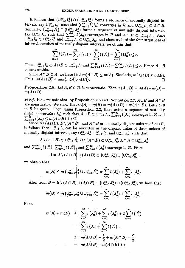
It follows that (U':'=lI~) n (U':'=lI~) forms a sequence of mutually disjoint in'-tervals, say U~lIn, such that E:=ll (In) converges in R and U~lIn C An B.Similarly, (U':'=l J~) n (U':'=l J~) forms a sequence of mutually disjoint intervals,say U~lJn, such that E~ll(J~) converges in R and AnB c U':'=lJn. SinceU':'=lIn C U~lI~ and U~lJn C U':'=lJ~, and since each of the four sequences ofintervals consists of mutually disjoint intervals,we obtain that

00 00 00 00

Ll(Jn) ~ Ll(In) 5: Ll (J~) -Ll(I~) 5: f.n=l n=l n=l n=l

Thus, U':'=lIn cAnE C U':'=lJn and E:=ll (In) -E:=ll (In) 5: f. Hence AnBis measurable.

Since AnB c A, we have that m(AnB) 5: m(A). Similarly, m(AnB) 5: m(B).Thus, m(AnB)'5: min{m(A),m(B)}. 0

Proposition 2.8. Let A, B c R be measurable. Then m(AUB) = m(A) +m(B)-m(AnB). c

Proof. First we note that, by Proposition 2.6 and Proposition 2.7, Au B and An Bare measurable. We show that m(A) + m(B) = m(A U B) + m(A n B). Let f > 0in R be given. Then, using Proposition 2.2, there exists a sequence of mutuallydisjoint intervals (In) such that A uB c U~l In, E:=ll(Jn) converges in RandE:=ll(Jn) 5: m(A U B)+ f/2.

Since A \ (AnB), B\ (An1J), and AnB are mutually disjoint subsets of AUB,it follows that U':'=l In can be rewritten as the disjoint union of three unions ofmutually disjoint intervals, say U':'=l J~, U':'=l J~, and U':'=l J~, such that

A\ (A nB) c ur:=lJ~,B \(A n B)c Ur:=lJ~,A n B C Ur:=lJ~,

and E:'=ll (J~), E:'=ll (J~)j! and E:'=ll (J~) converge inR. From

A = A\ (A n Br U (AnB) c (Ur:=lJ~) U(Ur:=lJ~) ,

we obtain that00 00

m(A) 5: m (Ur:=l{~U U':=1.J~) = L l(J~) + L l (J~).I n=l n=l

Also, from B = B \ (A n B) U (A n B) c (~':'=lJ~) U (U':'=l J~), we have that

00 00

m(B) 5: m(U':=lJ~UU':=lJ~) = Ll (j~) +Ll (J~).,

n=l n=l

Hence00 00 00

m(A) + m(B) 5: L l (J~) + L l (J~) + 2 L l (J~)n=l n=l n=l

00 00

=' Ll(Jn) + Ll{J~)n=l n=l

f f5: m(AUB)+2 +m(AnB) + 2

= m(AUB) +m(AnB)+f,

MEASURE THEORY AND INTEGRATION ON THE LEVI-CIVITA FIELD 377

where we have used the fact that00 00

Ll(J~) -m(AnB).$ Ll(Jn) -m(AUB).$~.n=l n=l

Thus, m(A) + m(B) .$ m(A U B) + m(A n B) + f for all f > 0 in n; and hence

(2.6) m(A) + m(B) .$ m(A U B) + m(A n B).

Now we prove the other inequality. Let t> 0 in n be given. Then, again byProposition 2.2, there exist a sequence of mutually disjoint intervals (J~) and asequence of mutually disjoint intervals (J;) such that A c U~~lJ~, B CU~=lJ;,En""=ll (J~) and En""=ll (J;) converge, and

00 00

Ll(J~) .$m(A)+~ and Ll(J~) .$m(B)+~.n=l n=l

Since B\(AnB) and AnB are mutually disjoint subsets of B, it follows that we canrewrite U~=l J; as the disjoint union of two unions of mutually disjoint intervals,say U~=lJ;,l and U~=lJ;,2, such that

B \ r AB) 00 ) 21 00 T2 2"n C Un=l n' ,AnB CUn=lJii' ,

and En""=ll (J;,l) and En""=ll (J;i2) converge in n. From

Au B = Au (B \ (An B)) C (U~=lJ~) U (U~==lJ~,l),

we obtain that00 00

m(A U B) $ m (U~==l.J~ u Uh""=l J~,l) = L l (J~) + L l (J~,l)n=l n=l

, 00

$ m(A) + ~ + L l (J~,l).n=l

Also, since AnB C U~=lJ;,2, we obtain that m(AnB) .$ En""=ll (J;,2). Hence00 00

m(AUB) +m(AnB) .$ m(A) + ~+ Ll(J~,l) + Et(J~,2)n=l n=l

00

= m{A) ~ ~+ L l (J~)n=l

f f< m(A )c+ -+ m(B )+ ~-2 " 2

= m(A) +m(B) + f.

This is true for all f > 0 in n; and hence

(2.7) m(AUB) +m(AnB).$ m(A) +m(B).Combining the results of Equation (2.6) and Equation (2.7), we obtain that

m(AUB)+m(AnB) = m(A)+m(B) or m(AUB) = m(A)+m(B)-m(AnB). 0

Finally, we note that the complement of a measurable set in a measurable setneed not be measurable. For example, [0,1] and [0,1] nQ are both measurable withmeasures 1 and 0, respectively. However, the complement of [0,1] n Q in [0,1] isnot measurable. On the other hand, if B C A C n and if A, B and A \ B are allmeasurable, then it follows from Proposition 2.6 that m(A) = m(B) + m(A \ B).

378 KHODR SHAMSEDDINE AND MARTIN BERZ

The example of [0,1] \ [0,1] n Q above shows that the axiom of choice is notneeded here to construct a nonmeasurable set, as there are many simple examplesof nonmeasurable sets. Indeed, any uncountable real subset of R, like [0, 1] n JR forexample, is not measurable.

3. MEASURABLE FUNCTIONS

Like in JR, we first introduce a family of simple functions on R from which wewill obtain a larger family of measurable functions.

3.1. Simple Functions. In the Lebesgue measure theory on JR, the simple func-tions consist only of step functions (piece-wise constant functions); and all measur-able functions including all monomials, polynomials and power series are obtainedas uniform limits of simple functions. It can be easily shown that in R the ordertopology is too strong and none of the monomials can be obtained as a uniformlimit of polynomials of lower degrees. So using the step functions as our simplefunctions would yield a too small class of functions that we can integrate. So weintroduce a larger family of simple functions. Here we define such a family of simplefunctions in an abstract way, which we will use throughout the discussions in thispaper; and we will give two examples in Remark 4.15 at the end of the paper..Definition 3.1. Let a < b in R be given and S(a, b) a family of functions fromI(a,b) to R. Then we say that S(a,b) is a family of simple functions onI(a,b) ifthe following are true:

(1) S(a, b) is an algebra that contains the identity function;(2) for all IE S(a, b), I is Lipschitz on I(a, b) and there exists an anti-derivative

F of I in S(a,b);(3) for all differentiable I E S(a, b), if I' = 0 on I(a, b) then I is constant on

I(a, b); moreover, if I' ~ 0 on I(a, b) then I is nonincreasing on I(a, b).If IE S(a, b), we say that I is simple ~n I(a, b).

It follows from the first condition in Definition 3.1 that any constant function onI(a, b) is in S(a, b); moreover, if], 9 E S(a, b) and if a E R, then 1+ ag E S(a, b).Also, it follows from the third condition that the anti-derivative in the secondcondition is unique up to a constant. A close look at Definition 3.1 reveals that thepolynomials algebra on I(a, b) is the smallest family of simple functions on I(a, b).Two examples of larger families of simple functions are discussed at the end of thepaper, in Remark 4.15.

While the third condition in Definition 3.1 is automatically satisfied in real anal-ysis, this is not the case in R, as the following example shows.

Example 3.2. Let 9 : (0,1) -+ R be given by g(x)[q] =x[q/3] for all q E Q. Then9 is differentiable on (0,1) with g'(X) = 0 for all x E (0,1). We first observe thatg(x + 'II) = g(x) +g('I/) for all x,y E (0,1). Now let x E (0,1) and f > 0 in R begiven. Let 8 = ~{E,d}, and let y E (0,1) be such that 0 < Iy -xl <8. Then

I g(y) -g(x) 1 I g(y-X) / 2 ., = ""(1/- x) sInce g(y -x) "" (y- x)3.y-x y-x

Since Iy -xl < min{f, d}, we obtain that (y -x)2 «f. Hence

Ig(y! -g(x} I< t; for all y E (0,1) satisfying 0 < jy -cxl <8;y-x '

MEASURE THEORY AND INTEGRATION ON THE LEVI-CIVITA FIELD 379

which shows that 9 is differentiable at x and g!(x) = O.Now let I : (0,1) -* R be given by I(x) = g(x) -X4. Then I is differentiable on

(0,1) with I'(x) = _4x3 < 0 for all x E (0,1). However, we have that d > ~ andI(d) = d3 -d4 > I(~) = fi6 -~. Thus, even though I' < 0 everywhere on (0,1),I is not nonincreasing on (0,1).

As we will see in Section 3.2, starting with the family of simple functions, wewill be able to obtain a larger family of measurable functions. Then, in Section 4,by just requiring the integral to satisfy one fundamental property, we show thatthere is only one way to define the integral of a simple function over an interval.Then, based on that, we show how to integrate any measurable function over ameasurable set.

3.2. Measurable Functions.

Definition 3.3. Let A c R be a measurable subset of R and let I : A -* R bebounded on A. Then we say that I is measurable on A if for all f > 0 in R, thereexists a sequence of mutually disjoint intervals (In) such that In C A for all n,L~=ll (In) converges in R, m(A) -L~=ll(In) ~ f and I is simple on In for all n.

Proposition 3.4 (Characterization of Measurable Functions). Let A C R be mea-surable and let I : A -* R be measurable. Then I is locally a simple function almosteverywhere on A.

Proof Let A1 = {x E A : I is not locally simple around x}. We show that Alis measurable and m(Al) = O. Let f > 0 in R be given. Then, since A ismeasurable and since I is measurable on A, there exist a sequence of mutuallydisjoint open intervals (an, bn) and a sequence of mutually disjoint intervals (In)such that U~=l(an,bn) C A c U~=lJn,.f is simple on {an,bn) for each n EN,L~=l (bn -an) and L~=ll(Jn) converge, m(A) -L~=l (bn -an) ~ f/2 andL~=ll(Jn) -m(A) ~ f/2. It follows that

A1 C A \ U'::=l(an,bn) C u..oo=lJn \ U~=l(an,bn),

where U~=l In \ U~=l (an, bn) can be written as a union of mutually disjoint intervals,say U~=l J!, such that E~=11 (J!) converges in R and }::::~11 (J!) = }::::~=ll( In)-}::::~=1 (bn -an)' For each n E N, let I~ = 0. Then U':=l.I~ C A1 <;: U':=lJ~ and

00 00 00 00 00

L l (J;) -L (I~) = L l (J~) = L l(Jn) -L{bn -a~)n=l n=l n=l n=l ..=1

= (f l(Jn) -m{A) ) + (m(A) -f(bn -an))n=l ni=l

f f< -+ -= f.-2 2

Thus, A1 is measurable. Moreover, since A1 c U':=lJ!, we obtain that m(A1) ~}::::~=ll (J~) ~ f. This is true for all f> 0 in Rj and hence m(A1) = O. 0

The following example shows that the converse of Proposition 3.4 need not betrue.Example 3.5. Let I : [0, II -* R be given by

I(x) = { 0 ifxE[?,ijnQ.x otherwlSe

380 KHODR SHAMS ED DINE AND MARTIN BERZ

Then f is locally simple almost everywhere on [0, I}; but f is not measurable on[0,1].

As an immediate result of Proposition 3.4 and the properties of simple functions,we obtain the following result which will prove very useful in defining the integralof a measurable function, as we will see in details in Section 4.

Corollary 3.6. Let a < b in R and let f : 1(a, b) -+ R be measurable. Then f iscontinuous almost everywhere on 1(a,b). Moreover, iff is differentiable on 1(a,b)and if f' vanishes everywhere, then f is constant on I (a, b).

Proof. The first part follows directly from Proposition 3.4 and the fact that a simplefunction is continuous everywhere on its domain.

Now assume that f is differentiable on 1(a, b) and that f(x) = 0 for all x E1(a, b). The~ it follows from Proposition 3.4 that f is locally constant almosteverywhere on 1(a, b); this is so since a simple function has a vanishing derivativeon a whole interval if and only if it is constant on that interval [11]. Thus, f islocally constant on 1(a, b) except on a discrete set of points in 1(a, b); and this,together with the fact that f is differentiable on 1(a, b), entails that f is constanton the whole interval 1(a, b). 0

Corollary 3.7. Let a < b in R and let f, 9 : [a, b} -+ R be measurable. Assume thatf and 9 are both differentiable with f = g' on [a, b]. Then there exists a constantc such that f(x) = g(x) + c for all x E [a,.b]; and hence f(b) -f(a) = g(b) -g(a).

Proposition 3.8. Let A, B c R be measurable, let f be a measurable function onA and B. Then f is measumble on Au B and An B.

Proof. Let f > 0 in R be given. Then, since f is measwable fon A, there existsa sequence of mutually disjoint intervals (1~) such that U':=l1~ C A, E'::=ll (1~)converges, m(A) -E'::=ll (1~) ~ f/2, and f is simple on 1~ fbr all n ?: 1. Also,since f is measurable on B, there exists a sequence of mutually disjoint intervals(I;) such that U':=l1; c B, ~~ll (I;) converges, m(B) -E'::=ll (I;) ~ f/2,

and f is simple on I; for all n ?: 1.It follows that (U':=lI~) U (U':=lI;) can be written as a union of mutually

disjoint intervals, say U':~l1n, such that U':=lIn = (U~lI~) U (U':=lI;) c Au B,~'::=ll (In) converges, and f is simple on In for all n ?: 1. Moreover,

00 00 00

f fm(AUB) -Ll (In) ~ m(A) -Ll (I~) +m(B) -Ll (I~) ~ "2 +"2 = f.

n=l n=l n=l

This shows that f is measurable on A U B.Also, (U':=l1~) n (U':=l1;) can be written as a union of mutually disjoint inter-

vals, say U':=lI~, such that U':=lI~ = (U':=lI~) n (U':=lI;) cAn B, ~'::=ll (I~)converges, and f is simple on ~ for all n ?: 1. Moreover, using Proposition 2.8, we

MEASURE THEORY AND INTEGRATION ON THE LEVI.CIVITA FIELD 381

have that(X)

m(A riB) -Ll (~) ~ m(A) + m(B) -m(A UB)n=1

(X) (X) (X)

+Ll(In) -L l (1~) -Ll (1~)n=1 n=l n=l

(X) (X)

f m(A) + m(B) -L l (1~) -L l (1~)..=1 n=1

(X) (X)

:i::: m(A) -L l (I~) + m(B) -L l (1~)n=1 n=1

f f.

Thus, I is measurable on An B. 0

Proposition 3.9. Let A c R be measurable, let I, 9 : A -+ R be measurable andlet a E R be given. Then I + ag and I .9 are measumble on A.

Proal. Let f > 0 in R be given. Then there exist a sequence of ~utually disjointintervals (I;) and a sequence of mutually disjoint intervals (I;) suph that U'":'=1 I; cA, U'":'=11; c A, ~'::=1l (I;) and ~~1l (I;) converge, m(A) -E'::=1l (I;) $ f/2,m(A) -~'::=1l (I;) $ f/2, I is simple on I; for all n E N and 9 i* simple on I; forall n E N. !

It follows that (U'":'=11;)n(U'":'=1I;) can be written as a union ofimutually disjointintervals, say U'":'=1~' such that U'":'=11~ = (U'":'=11;) n (U'":'=11;) c A'~'::=1l (1~)converges, and 1+ ag and I. 9 are simple on ~ for all n ? 1 (where we use the factthat the sum and product of simple functions are again simple). Moreover, againusing Proposition 2.8, we have that

(X) (X) (X)

m(A) -Ll (1~) = m(A)+m (U~=l1;UU~=lI;) -Ll (I~) -Ll (I;)n=1 n=1 n=1

(X) (X)

$ m(A) + m(A) -L l (I;) -L l (1~)n=1 n=1

(X) (X)".""'= m(A) -L l (1~) + m(A) -L l (1~)

n=1 n=1f f< -+ -= f.

-2 2

Thus, I + ag and I .9 are measurable on A. 0

The following example shows that the uniform limit of measurable functions neednot be measurable.

Example 3.10. For each kEN, let Ik : [0,1] -+ R be given by Ik(X) = dj ifx belongs to one of the open intervals deleted from [0, 1] at the jth step of theconstruction of the real Cantor set C for 1 $ j $ k, and Ik(X) = dk+1 if x belongsto the closed set left from [0,1] at the kth step of the construction of C. Then thesequence (Ik) converges uniformly on [0,1]; but the limit function is not measurableon [0,1]. The proofs of the last two statements are left as an exercise for the reader.

-

382 KHODR SHAMSEDDINE AND MARTIN BERZ

4. INTEGRATION

After having introduced measurable functions and studied their properties inSection 3, we show in this section how to find the measure or integral of a givenmeasurable function f over a measurable set A, which we will denote by J A f.However we define the integral, we would like it to satisfy as many of the basicproperties of real integrals as possible. One such fundamental property of realintegrals is that the integral of the derivative of a differentiable function over aninterval is equal to the difference between the function values at the endpoints. Byrequiring just that, namely that

(4.1) r f = f(b) -f(a)J[a,b]

for a differentiable measurable function f on [a, b] (which is a well-defined require-ment by Corollary 3.7), then we will show that there is only one way to define theintegral of any measurable function f over any measurable set A c n.

First assume that f :I(a, b) -+ n is simple and let F be a simple anti-derivativeof f on I(a, b). Then F is measurable and differentiable on I(a, b). If I(a, b) isclosed, we use Equation (4.1) and define the integral of f over I(a,b) = [a,b] asF(b) -F(a). If I(a, b) is not closed, then we can extend F to a new simple functionF: [a,b] -+ n, such that

{ F(x) if x E (a, b).F(x) = limx--+a F(x) if x = a .

limx-+b F(x) if x = b

Then F is an anti-derivative of 1, the extension of f on [a, bj. So it is natural inthis case to require that J I(a,b) f = J[a,b] 1; which leads to

r f = F(b) -F(a) = lim F(x) -lim F(x!).J I(a,b) x-+b x--+a

That the limits in defining the extensions exist follow from the fact that thesimple functions are Lipschitz. We combine the two cases above (closed interval orotherwise) into one expression and define the integral of a simple function over aninterval.

Definition 4.1. Let a < bin n, let / : I(a, b) -+ n be simple on I(a, b), and letF be a simple anti-derivative of f on I(a, b). Then the integral of / over I(a, b) isthe n number

r / = lim F(x) -lim F(x).J I(a,b) x--+b x--+a

The following result is an immediate consequence of Definition 4.1.

Proposition 4.2. Let a < b in n and let a E n be a given constant. ThenJI(a,b) a = a(b -a).

Proof. First we note that ax is a simple anti-derivative of the constant function aon I(a, b). Thus, JI(a,b) a = limx--+b(ax) -limx--+a(ax) = a(b -a). 0

Proposition 4.3. Let a < b in n, let /,g : I(a,b) -+ n be simple, and let a Enbe given. Then JI(a,b) (J + ag) = JI(a.,b) / + a J1(a,b) g.~

, .

MEASURE THEORY AND INTEGRATION ON THE LEVI-CIVITA FIELD 383

Proof Let F and G be simple anti-derivatives of f and 9 on I(a, b), respectively.Then F +aG is an anti-derivative of f + ag on I(a, b). Thus,

[ (f + ag) = 1im(F + aG)(x) -lim(F + aG)(x)J I(a,b) x-+b x-+a

= lim(F(x).+ aG(x)) -lim(F(x) + aG(x))x-+b x-+a

= (lim F(x) -lim F(X) ) + a (lim G(x) -lim G(X) )x-+b x-+a x-+b x-+a

= [ f + a [ g.J I(a,b) J I(a,b)

0

Proposition 4.4. Let a < b in R, let f : I(a, b) --t R be simple and nonpositiveon I(a, b). Then JI(a,b) f ::; O.

Proof Let F be a simple anti-derivative of f on I(a, b). Then JI(a,b) f = limx-+b F(x)-limx-+a F(x). Since F' = f ::; 0 on I(a., b), F is nonincreasing on I(a, b). It followsthat limx-+b F(x) ::; limx-+a F(x); and hence JI(a,b) f ::; o. 0

Using Proposition 4.3 and applying Proposition 4.4 to f -g, we readily obtain:

Corollary 4.5. Let a < b in R, let f, 9 : I(a, b) --t R be simple and satisfy f ::; 9on I(a, b). Then JI(a,.b) f ::; JI(a,b) g.

Corollary 4.6. Let a < b in R, let f : I(a, b) --t R be simple on I(a, b) and let Mbe a bound of If I on I(a, b). Then

I [ fl ::; M{b -a).

JI(a,l»

Proof Using Corollary 4.5 and the fact that f ::; Iii::; M on I(a, b), we obtainthat

(4.2) [ f::; [ M = M(b -a).

JI(a,b) JI(a,b)

Also noting that -f::; If I ::; M on I(a,b), we obtain that

(4.3) -[ f = [ (- f) ::; M(b -a).J I(a,b) J I(a,b)

Combining the results of Equation (4.2) and Equation (4.3), we finally obtain thedesired result. 0

Now let A c R be measurable, let f : A ~ R be measurable and let M be abound for If I on A. Then for every kEN, there exists a sequence of mutuallydisjoint intervals (I~)nEN such that ur;:>=lI~ c A, E'::=11 (I~) converges, m(A) -

E'::=11 (I~) ::; dk, and f is simple on I~ for all n E N. Without loss of generality, wemay assUllle that I~ c I~+l for all n E N and for all kEN. Since limn-+co l (I~) = 0,

and since IJI~ fl ::; Ml (I~) by Corollary 4.6, it follows that

lim [ f = 0 for all kEN.n-+co J Ik

n

-

..

384 KHODR SHAMSEDDINE AND MARTIN BERZ

Thus, E'::=l Ilk f converges in R for all kEN [11].n

Next we show that the sequence (E'::=l II~ f) kEN converges in R. So let E > 0

be given in R; and let KEN be such that M dK ::; E. Let k > j :;:::: K be given in

N. Then U':=l I~ \ U':=l I~ can be written as a union of mutually disjoint intervals,

say (I~,k)nEN' such that E'::=ll (I~,k) converges, and

00 00 00 00

L I (I~,k) = L I (I~) -L I (I~) ::; m(A) -L I (I~) ::; dj ::; dK.

n=l n=l n=l n=l

Thus,

I~i~f-~i;!.fl= I~i;!.'kfl ::;~Ii;!.'kfl00 00

::; L MI (I~.k) = M LI (I~,k)

n=l n=l

::; M dK ::; E,

where we have used the fact that an infinite series converges if and only if it con-

verges absolutely [11]. Thus, the sequence ( Eoo=l Ilk f ) is Cauchy; and hencen n kEN

it converges in R. We define the unique limit as the integral of f over A.

Definition 4.7. Let A c R be measurable and let f : A -+ R be measurable.

Then the integral of f over A, denoted by I A f, is given by1 00 f = lim f.

A }::;';:'=\.!(In) -+ m(A) ~ inUn=lIn C A n-l

(In) are mutually disjointf is simple on In 'V n

Proposition 4.8. Let A c R be measurable and let a E R be given. Then I A a =

am(A).

Proof. Using Definition 4.7, we have that1 00 1. 00 a = lim a = lim al(In)

A }::;';:'=\.!(In) -+ m(A) ~ In }::;';:'=\.!(In) -+ m(A) ~Un=l In C A Un=l In C A

(In) are mutually disjoint (In) are mutually disjoint00

= a lim L I(In) = am(A).}::;~1 I(In) -+ m(A)

""" A n-lUn=l In C -(In{ are mutually disjoint

In particular, we have that m(A) = IA 1. m

Proposition 4.9. Let A c R be measurable and let f : A -+ R be measurable and

nonpositive on A. Then IA f ::; O.

Proof. Let E > 0 in R be given. Then there exists a sequence of mutually disjoint00 00

intervals (In) such that U':=lIn C A, En=ll (In) converges, m(A) -En=ll (In) ::;

E, and f is simple on In for all n E N. It follows, using Proposition 4.4, thatE'::=l IIn f ::; 0; and hence IA f = lime-o E'::=l IIn f ::; O. 0

, .

MEASURE THEORY AND INTBGRATION ON THE LEVI-CIVITA FIELD 385

Using the proof of Proposition 3.9 and a limiting argument similar to that in theproof of Proposition 4.9, we obtain:

Proposition 4.10. Let A c R. be measurable, let f,g:A~ R. be measurable, andlet a E R. be given. Then fA U + ag) = fA f + afAg.

As a consequence of Propositions 4.9 and 4.10, we obtain the following result.

Corollary 4.11. Let A c R. be measurable and let f,g : A ~R. be measurable andsatisfy f ~ 9 on A. Then fA f ~ fA g.

Corollary 4.12. Let A c R. be measurable, let f : A ~ R. be measurable and letM be a bound for If I onA. Then If A fl ~ Mm(A).

Using the proof of Proposition 3.8, and using the limiting argument in the proofof Proposition 4.9, we obtain the following result.

Proposition 4.13. Let A, B c R. be measurable and let f be a measurable functionon A and B. Then

[ f = [f + [ f -f f.JAUB JA JB JAnB

Theorem 4.14. Let A c R. be measurable, let f : A ~ R., for each kEN letfk : A ~ R. be measurable on A, and let the sequence Uk) converge uniformlyto f on A. Then limk-.oo fA fk exists. Moreover, if f is measurable on A, thenlimk-.oo fA fk = fA f.

Proof. Let f > 0 in R. be given and let

f = { fjm(A) if m(A) #0 .I f ifm(A) = 0

Then fl > 0 and there exists KEN such that Ifk(X) -fj(j;)I!~ ~l for all k,j ~ KIand for all :t E A. It follows that

Ii fk -i fjl = li Uk -fj)l~ flm(A) ~ f for all k,j ~ K.

Thus, the sequence (fA fk) is Cauchy. Since R. is Cauchy complete in the ordertopology, the sequence (fA fk) converges in R.j that is, limk-.oo fA fk exists in R..

Now assume that f is measurable on A; to show that limk-.OQ fA fk = fA f, wefollow the same steps as in the first part of the proof, replacing f j by f. 0

Remark 4.15. Power series [11, 12] are one example of a family of simple functions onany interval in their domain of convergence. Prior to [11, 12], work on power serieson the Levi-Civita field has been restricted to power series with real coefficients.In [5, 6, 7, 4], they were studied for infinitely small arguments, while in [1], usingthe weak topology, also finite arguments were possible. In [11], the general case ofR. coefficients and arguments is considered. A radius of convergence 7] is derivedsuch that the power series converges weakly for all points whose distance from thecenter is finitely smaller than 7] and it converges strongly (in the order topology)for all points whose distance from the center is infinitely smaller than 7].

In [12] it is shown that within their radius of convergence, power series are infin-itely often differentiable and the derivatives to any order are obtained by differenti-ating the power series term by term. Also, power series can be re~expanded aroundany point in their domain of convergence and the radius of convergence of the new

.' I

386 KHODR SHAMSEDDINE AND MARTIN BERZ

series is equal to the difference between the radius of convergence of the originalseries and the distance between the original and new centers of the series. Fur-thermore, it is shown in [11, 12] that power series satisfy all the common theoremsof real calculus on a closed interval of R, like the intermediate value theorem, themaximum theorem and the mean value theorem and that they satisfy the criteriafor a family of simple functions on any interval in their domain of convergence.

Research currently in progress aims at generalizing the results in [11, 12] topower series with rational exponents. We show that unless the, coefficients in theseries form a null sequence in the order topology, the sequence of exponents must beleft-finite for the series to have a positive radius of convergence. In the latter case,we derive a radius of convergence which depends on the density of the exponentsand on the coefficients in the series.

We then show that within their domain of convergence, generalized power serieswith rational exponents have similar properties to those of regular power series. Inparticular, they satisfy the intermediate value theorem and the mean value theoremand they can be re-expanded around any point in their domain of convergence.We also show that the generalized power series with rational exponents satisfythe criteria for a family of simple functions on any interval in their domain ofconvergence.

REFERENCES

[1] M. Berz. Calculus and Numerics on Levi-Civita Fields. In M. Berz, C. Bischof, G. Corliss, andA. Griewank, editors, Computational Differentiation: Techniques, Applications, and Tools,pages 19-35, Philadelphia, 1996. SIAM.

[2] M. Berz. Analytical and Computational Methods for the Levi-Civita Fields. In Lecture Notesin Pure and Applied Mathematics, pages 21-34. Marcel Dekker, Proceedings of the SixthInternational Conference on P-adic Analysis, July 2-9, 2000, ISBN 0-8247-0611-0.

[3] Wolfgang Krull. Allgemeine Bewertungstheorie. J. Reine Angew. Math., 167:160-196, 1932.[4] D. Laugwitz. Thllio Levi-Civita's work on nonarchimedean structures (with an Appendix:

Properties of Levi-Civita; fields). In Atti Dei Convegni Lincei B: Convegno InternazionaleCelebmtivo Del. Centenario Della Nascita De Thllio Levi-Civita, Academia Nazionale deiLincei, Roma, 1975.

[5] Thllio Levi-Civita. Sugli infiniti ed infinitesimi attuali quali elementi analitici. Atti 1st. Venetodi Sc., Lett. ed Art., 7a, 4:1765, 1892.

[6] Thllio Levi-Civita. Sui numeri transfiniti. Rend. Acc. Lincei, 5a, 7:91,113, 1898.[7] L. Neder. Modell einer Leibnizschen Differentialrechnung mit aktual unendlich kleinen

GraBen. Mathematische Annalen, 118:718-732, 1941-1943.[8] S. Priess-Crampe. Angeordnete Strukturen: Gruppen, Ko771er, projektive Ebenen. Springer,

Berlin, 1983.[9] Paulo Ribenboim. Fields: Algebraically Closed and Others. Manuscripta Mathematica,

;5:115-150,1992.110J K. Sh~seddine. New Elements of Analysis on the Levi-Civita Field. PhD thesis, Michigan

State University, East Lansing, Michigan, USA, 1999. also Michigan State University reportMSUCL-1147.

[II] K. Shamseddine and M. Berz. Convergence on the Levi-Civita Field and Study of PowerSeries. In Lecture Notes in Pure and Applied Mathematics, pages 283-299. Marcel Dekker,Proceedings of the Sixth International Conference on P-adic Analysis, July 2-9, 2000, ISBN0-8247-0611-0.

[12] K. Shamseddine and M. Berz. Analytical Properties of Power Series on Non-ArchimedeanFields. submitted. see also Michigan State University report MSUCL-ll63.

-1 , ~

MEASURE THEORY AND iNTEGRATION ON THE LEVI-CIVITA FIELD 387

DEPARrMENT OF MATHEMATICS AND DEPARTMENT OF PHYSICS AND ASTRONOMY, MICHIGANSTATE UNIVERSITY, EAST LANSING, MI 48824

E-mail address: khodriDmath.msu.edu

DEPARTMENT OF PHYSICS AND ASTRONOMY, MICHIGAN STATE UNIVERSITY, EAST LANSING, MI

48824E-mail address: berziDmsu. edu