i

Measurement of frontal area of

athletes in wind tunnel experiments

Lars Morten Bardal

18.12.09

Department of Energy and Process Engineering

i

Preface This report is the result of my specialisation study performed at the department of Energy

and Process Engineering at the Norwegian University of Science and Technology during the

fall of 2009. The main objective for the project was to develop a laboratory computer tool to

estimate the frontal area and drag coefficient of athletes in wind tunnel experiments.

The work with this project has been both interesting and challenging for me, especially since

the programming part of the project is somewhat outside my field of knowledge. It has

however been developing for me to expand my knowledge and learn some basic LabVIEW

programming.

At last I would like to thank my supervisor Luca Oggiano for all the support, helpful ideas and

good cooperation during the development and testing of the program.

ii

Sammendrag Innen idrettsforskningen har det de siste årene blitt lagt økende grad av vekt på

optimalisering av aerodynamiske egenskaper for utøvere av høyhastighets idretter da disse

har stor innvirkning på prestasjonen når marginene blir mindre. Aktuelle idretter for slik

optimalisering er skøyteløp, vei- og banesykling, alpine skiidretter og skihopping. Et viktig

redskap for måling og reduksjon av aerodynamiske motstandskrefter er vindtunnelmålinger.

Motstandskraften som blir målt er avhengig av touavhengige parametre; drag koeffisienten

og frontalarealet, dersom vindhastighet og lufttetthet blir holdt konstant. For å gi et korrekt

estimat av drag koeffisienten må derfor frontalarealet måles.

Målet for dette prosjektet var å utvikle og teste et dataprogram som var i stand til å måle

frontalarealet i sanntid ved bruk av et videokamera, og samtidig måle motstandskraft og

vindhastighet for å kunne gi et estimat av CD i sanntid. Programmet ble basert på det grafiske

programmeringsgrensesnittet LabVIEW fra National Instruments. Prinsippet som ble

benyttet for å trekke ut arealet av utøveren var taktisk lyssetting, som skulle gi en kontrast

mellom utøveren og bakgrunnen.

Det ble utført grundige tester av programmet i en storskala vindtunnel for å evaluere og

validere arealmålingene fra programmet. Til testingen ble det benyttet en modell med fire

ulike skøyteløpsdrakter med ulike reflektive egenskaper. Testresultatene viste at en nøyaktig

lyssetting av objektet var avgjørende for å gi et nøyaktig estimat av arealet. Videre viste det

seg at metoden har visse svakheter når det gjelder reflektive egenskaper hos både objektet

og bakgrunnen. Test resultatene var både konsistente og stabile for tre av draktene, men

med et avvik fra det virkelige arealet på omkring 20%. Med enkelte forbedringer av test

oppsettet og bakgrunnen ser det imidlertid ut til at programmet kan bli et nyttig verktøy i

eksperimentelt laboratoriearbeid.

iii

Abstract In the field of sports science a lot of effort is put into optimizing of the aerodynamic

properties of athletes in high speed sports. Such sports include for instance speed skating,

road- and track cycling, alpine skiing and ski jumping. An important tool in measuring and

reducing the aerodynamic drag forces on the athlete is wind tunnel measurements. The drag

force which is measured in such experiments depends on two independent parameters; the

drag coefficient and the projected frontal area, given stable wind speed and air density. In

order to correctly estimate the drag coefficient, the frontal area of the athlete will therefore

have to be calculated.

The objective of this project was to develop and test a computer program that was able to

calculate the frontal area in real time measurements using a video camera. The program

would also acquire drag and wind speed data in order to provide a real time CD estimate. The

program was based on a graphical programming language called LabVIEW from National

Instruments. The basic idea for the extraction of area was to create a contrast between the

object measured and the background using tactical illumination.

Tests were performed in a large scale wind tunnel, using four different speed skating suits,

to evaluate and validate the area measurements performed by the program. The test results

showed that an accurate illumination of the object is crucial for getting accurate

measurements. Also the method has some limitations regarding reflective properties of both

the measured object and the background. The test results were consistent and stable, but

about 20 percent inaccurate for three of the four suits tested. With some improvements of

the testing environment and setup the program would have the potential to be very useful

in laboratory experimental work.

iv

Table of Contents Preface ...................................................................................................................................................... i

Sammendrag ............................................................................................................................................ii

Abstract ................................................................................................................................................... iii

List of figures ............................................................................................................................................ v

Introduction ............................................................................................................................................. 1

About LabVIEW ........................................................................................................................................ 2

The Program ............................................................................................................................................ 3

VI Hierarchy ......................................................................................................................................... 3

Main VI ................................................................................................................................................ 4

Front panel ...................................................................................................................................... 4

Block diagram .................................................................................................................................. 5

Calibration VI ....................................................................................................................................... 8

Front panel ...................................................................................................................................... 8

Block diagram .................................................................................................................................. 8

Pixel count VI ....................................................................................................................................... 9

Block diagram .................................................................................................................................. 9

Testing and validation ........................................................................................................................... 10

Test procedure .................................................................................................................................. 10

Test results ........................................................................................................................................ 12

Discussion .......................................................................................................................................... 17

Conclusion ......................................................................................................................................... 18

Recommendations for improvements .................................................................................................. 19

References ............................................................................................................................................. 20

v

List of figures

Figure 1 VI hierarchy................................................................................................................................ 3

Figure 2 Main front panel ........................................................................................................................ 4

Figure 3 Main block diagram ................................................................................................................... 5

Figure 4 Block diagram function blocks ................................................................................................... 5

Figure 5 Calibration block ........................................................................................................................ 7

Figure 6 Time delay block ........................................................................................................................ 7

Figure 7 Calibration VI front panel .......................................................................................................... 8

Figure 8 Calibration VI block diagram ..................................................................................................... 9

Figure 9 Pixel count block diagram ......................................................................................................... 9

Figure 1 Test setup ................................................................................................................................ 10

Figure 2 Example of reference method vs. LabVIEW method .............................................................. 10

Figure 3 Test suits .................................................................................................................................. 11

Figure 4 Test postures ........................................................................................................................... 11

Figure 5 Red suit (suit 2) measurement series ...................................................................................... 12

Figure 6 Black suit (suit 4) measurement series .................................................................................... 12

Figure 7 Upright position validity .......................................................................................................... 13

Figure 8 Middle position validity ........................................................................................................... 13

Figure 9 Low position validity ................................................................................................................ 13

Figure 10 Measurement deviation from reference ............................................................................... 14

Figure 11 Measurement consistency .................................................................................................... 14

Figure 12 Measurement variation ......................................................................................................... 15

Figure 13 CDA vs. Area ........................................................................................................................... 15

Figure 14 CDA 7m/s ................................................................................................................................ 16

Figure 15 CDA 14 m/s ............................................................................................................................. 16

1

Introduction In the field of sports science huge effort is made to optimize technical equipment in order to

improve performance. Even very small technical improvements can make the difference

between an outstanding and an average performance when the margins are small. Especially

in high-speed sports, such as speed skating, alpine skiing, cycling and ski-jumping the

benefits of reduced resistive forces are substantial. The single most important resistance

parameter in these sports is aerodynamic drag (van Incen Schenau, 1982; Grappe et al.,

1997). Wind tunnel measurements are, due to this fact, commonly used to optimize the

athletes’ aerodynamic properties, such as clothing and body posture.

The drag force on a body in a fluid field:

where ρ is the air density, CD is the dimensionless drag coefficient, A is the projected frontal

area and U is the free stream velocity. Since the drag is proportional to the square of the

velocity, aerodynamic properties become increasingly dominant with higher speed. CD is

dependent on the shape and surface structure of the body and must be determined through

experiments.

In order to determine CD correctly, the projected frontal area must be determined with high

precision. In experiments involving drag on complex geometries, such as athletes, the

common solution is to determine the area by still-image post processing. There are several

post processing methods used. Older studies either rely on the method of weighing

photographs (Swain et al., 1987), or manually analysis using a reference length scale (van

Incen Schenau, 1997). These methods are both time- and work-demanding and inaccurate.

More recent studies use different types of computer based analysis: post-digitizing (Heil,

2001), computer aided design software (CAD) (Meile et al., 2006; Debraux et al., 2008),

digitizing (Debraux et al., 2008). A drawback of these methods is the need of post-

processing. The drag D and the wind speed U can both be measured in real time. Therefore a

real time measurement of the frontal area would give continuous CD measurements, and

thereby valuable feedback for both the athletes being tested and the researcher.

The goal for this project is to develop and test a laboratory computer tool which implements

real time area measurement with drag force and wind speed acquisition in wind tunnel

experiments. Labview from National Instruments is chosen as programming tool due to its

data acquisition capabilities, image processing opportunities and user friendly interface.

2

About LabVIEW LabVIEW is a commercial, graphical programming language introduced by National Instruments in

19861. It was originally developed for laboratory research applications and mainly for data acquisition

and experiment automation, but has later grown to cover a large range of test-, measurement- and

control applications in both research and industry. Today the LabVIEW platform offers functionality

for a number of different appliances such as internet- and database connectivity, FPGA-

programming, and image processing2.

The LabVIEW programming language is basically dataflow based. The programming environment,

called block diagrams, consists of a number of nodes called virtual instruments (VI) and a set of wires

to connect one node to another. The wires represent the dataflow concept and the function of a

node is executed once all needed input data is available. Basic programming functions such as loops

and if-else statements are handled by structure blocks in the block diagram. The user interface

environment of a VI is called the front panel, and is inspired by the appearance of a real laboratory

instrument with switches, buttons, knobs and indicator panels. Any user created VI can also run as a

subroutine (as a sub VI) of another VI with connectors from the front panel as input and output

parameters. This allows the user to divide the program into individual and independent parts that

can be used for other appliances later. The LabVIEW built-in libraries and toolkits contain a large

number of predefined functions for advanced data acquisition and processing. The Vision toolkit

contains functions for image acquisition and processing that is utilized in this project. An essential

benefit with LabVIEW is the ability to easily connect and acquire data from multiple sources

simultaneously using a data acquisition card (DAQ-card). The DAQ-card can acquire data from

multiple analog or digital channels simultaneously and all the data can readily be processed and

analyzed in LabVIEW3.

1 http://www.ni.com/company/history.htm (16.12.09)

2 http://www.ni.com/labview/ (16.12.09)

3 http://www.ni.com/dataacquisition/whatis.htm (16.12.09)

3

The Program The program package consists of 3 custom VI’s: the main program and two sub VI’s:

Main VI is the top of the VI hierarchy. It contains the main user interface with

all measurement controls and indicators for the processed data. The other custom sub VI’s is

called by this VI during run time. This VI also controls image- and data acquisition, image

processing, mathematical calculations, mean sampling and saving of data.

Calibration VI performs calibration of all parameters

needed for computations of area, drag and speed. The calibration VI is called by the main VI

and opens a separate front panel used for the user controlled calibration.

Pixel count VI takes a greyscale image as input, and calculates

the number of pixels above or below a given threshold limit given by the user. The output

from the pixel count VI divided by the pixels per square meter resolution from the

calibration VI gives the area.

VI Hierarchy

Figure 1 VI hierarchy

The VI hierarchy shows the VI’s used and how the VI calls are performed. The two custom sub VI’s

appear to the left in the figure. The rest of the sub VI’s are LabVIEW library VI’s.

4

Main VI

Front panel The main VI contains the main user interface (front panel) of the program, from which all user

interaction is controlled during measurements. The front panel consists of a number of controls and

indicators that receive and display information while the program runs. The front panel (shown in

Figure 2) is divided into sections with regard to functions. The upper left box controls the call of the

calibration VI, and displays calibration information after the calibration is done The “calibrate”

button loads the calibration VI and the calibration status lamp is illuminated when the calibration is

completed. The lower left box controls the measurement mode of the program and displays

measurement information when data is acquired. The “measure area” switch controls the

measurement loop in the block diagram and will only function when the calibration is done. The

indicator lamp will illuminate when the measurement is running. The “DAQ status” lamp states

whether or not the DAQ assistant is functioning properly and becomes red when a DAQ error occurs.

The lower box controls the sampling function and sampling parameters and displays the latest

sample. The “sample” button starts a sample of the time given in the “sample length” control. At the

first sampling since program start-up the user is asked to specify a directory and name for the

measurement file. The rate at which data is acquired [Hz] and the size of the data buffer [samples] is

controlled by the two controls under the sample button. The middle box contains image processing

controls and the threshold selector. The BCG control is a pre processing tool that lets the user adjust

the image to give a better separation. Since the program is based on greyscale image processing the

colour plane control will have to control what colour plane to extract from the captured RGB image.

The threshold control indicates the limit of the pixel value at which the pixels should be separated.

The control runs from 0 (black) to 255 (white) since the program works with 8-bit images. The left

image display shows the captured image as is or with a mask. This display is also used to select a

region of interest in the captured image. This is done with a rectangular ROI selector (click and drag).

The right image display shows the selected region of interest as a greyscale or binary image. It also

contains a control for a snapshot function.

Figure 2 Main front panel

5

Block diagram The block diagram of the main VI is divided in three chronological sections implemented as a flat

sequence. The first frame performs initialization of parameters and images. The second frame is the

run time frame and contains loops that run until the program is terminated. The third frame

performs disposal of image data and frees up used image memory when the program is stopped

using the stop button on the front panel. The run time frame contains a stacked sequence structure

inside a while loop that is active while the program is running. The stacked sequence contains

true/false structures for calibration and measurement mode and a timing node to free CPU capacity.

The false cases of all the boolean structures is either empty or image throughput.

Figure 3 Main block diagram

Figure 4 Block diagram function blocks

6

The functionality of the block diagram as shown in Figure 4:

1. Initialization block

Sets default values and allocates image memory

2. Data acquisition and calculation block

Continuously acquires pressure and drag force raw voltages from the connected

acquiring card when the program runs in measurement mode. Two formula nodes

connected to the DAQ assistant and the calibration cluster calculates wind speed and

drag force values

3. Sampling block

User activated block that makes a specified time sample of the collected data and

calculates the mean value. The sample mean values are saved to file with directory

specified by the user

4. Image acquisition block

Continuously acquires images from the selected camera when the program runs in

measurement mode

5. CD calculation node

Calculates and displays the continuous CD measurement

6. Image processing block

Creates a greyscale image from the desired colour plane and applies a BCG-control

palette

7. ROI extraction block

Extracts the user created ROI (Region of interest) from the image and applies to the

second image display

8. Threshold mask block

Applies a black mask to all pixels of vale lover than the given limit

9. Area calculation node

Calculates the actual area from the number of pixels selected

10. Binary image tool

Creates and displays a binary image that shows the actual measured pixels in the

second image display

11. Snapshot tool

Creates and saves a snapshot of the current frame displayed in the second image

frame when activated by the user

12. Image disposal block

Performs disposal of image data and frees up allocated memory

7

Figure 5 Calibration block

Figure 6 Time delay block

Figure 5 shows the calibration block of the stacked sequence. This block is activated when the user

presses the calibration button on the front panel. The program prompts the user for confirmation

and then acquires an image from the selected camera which is used as input for the calibration VI.

The calibration VI is called and automatically opens a separate front panel. The return data from the

calibration is saved as local variables in the main VI. The last frame of the stacked structure is just a

timing block which makes the program wait a given amount of time before the next iteration to free

processor capacity.

8

Calibration VI The calibration VI is called calibration.vi and is created as a sub VI with one input, three outputs and a

separate active front panel. The VI takes a RGB image as input and outputs a “pixel per meter”

double precision value, a cluster of calibration variables and a boolean value called “completed”.

Front panel The Calibration front panel opens automatically when the VI is called. The panel basically consists of

two sections, the image calibration section and the drag/speed device calibration section. The

drag/speed calibration parameters are manually adjusted with exception of the voltage offset values

which are sampled on users’ request. The image calibration is preformed manually with a calibration

sheet or frame with sharp contrast edges of known dimensions. Before the calibration VI is loaded a

calibration sheet is positioned at the centre of the measurement volume. Then user makes a line that

crosses two high contrast edges with a line ROI tool. The distance in pixels is between the edges is

then displayed in the “ROI pixels” indicator box. When the user presses the “Register ROI” button the

sample is saved and displayed in the “Edge sample” array under the image display. The actual

distance in measured in meters between the edges on the sheet is set in the “Distance between

edges” control. It’s recommended to use a large scale calibration sheet and take multiple samples in

order to minimize the calibration error. The calibration is complete when the number of set samples

equals the number of registered samples. The VI then prompts the user to close and sends the

collected parameters to the main VI.

Figure 7 Calibration VI front panel

Block diagram The block diagram of the calibration VI is constructed in a similar way as the main VI. It’s a flat

sequence of three frames where the first frame is an initialization frame where the default

parameters are set and the image is pre processed. The second frame is the sampling frame where

the samples, on which the calibration is based, are made. The third frame calculates the metric

9

definition of the image (pixels per meter) and creates a cluster of the remaining calibration

parameters. When all calculations are done the user is asked to close the front panel.

Figure 8 Calibration VI block diagram

Pixel count VI The pixel counting VI called pixcount.vi does not have an active front panel and this therefore a pure

sub VI. The VI has three inputs and one output. The inputs consists of a greyscale image, an integer

limit value which sets the pixel value limit of the counting and an integer of 0 or 1 which determines

whether to count the darker or the brighter pixels. The output is an integer number of pixels. The VI’s

basic function is to find the number of pixels in an image that is either brighter or darker than a given

pixel value.

Block diagram The pixel count VI is like the main and calibration VI’s also based on a chronological flat structure,

with an initialization frame, a calculation frame and a termination frame. The image input is

converted to a two dimensional array of pixel values. Two nested for loops are set to run through the

complete array. Each pixel value is evaluated and the pixels that satisfies the given condition is

summed up and returned to the calling VI.

Figure 9 Pixel count block diagram

10

Testing and validation

Test procedure The complete program was tested in a wind tunnel with force-, pressure and area measurement. A

test subject posing in four different speed skating suits in three different positions formed the basis

of the collected data. The test setup consisted of a simple USB web-camera connected to a laptop, a

force plate used to measure the drag force, a pitot tube used to measure the dynamic pressure and

four lamps to illuminate the test subject. The resolution of the camera was set to 640×480 and the

camera was placed vertically in approximately half the height of the subject standing up.

The test was performed in two sessions. The first session was carried out with area measurement

only. As a reference method of area measurement, manual area extraction with image processing

software was chosen. A Canon 350D DSLR was used to capture reference photographs during this

session. The frontal area was later extracted using Photoshop and used for validation of the results.

Three samples were made per position and suit. The second test session was carried out with drag-

and speed measurement with the tunnel running at two different speeds. Five samples were made

per suit, position and wind speed. All the data from the test is 3 second sample averages. Figure 16

through Figure 20 is taken from the first session while Figure 21 through Figure 24 is taken from the

second session.

Figure 10 Test setup

Figure 11 Example of reference method vs. LabVIEW method

11

Figure two shows the raw picture from the Canon 350D, the area extracted in photoshop and the

area measured by the LabVIEW program. Notice that the webcam image suffers from low resolution

and significant noise.

Figure 12 Test suits

Figure 2 shows the speed skating suits used in the test session. The four suits are later referred to as

suit 1-4 as shown from the left in the figure.

Figure 13 Test postures

Figure 2 shows the three different test postures used in the test session. The postures are later

referred to as the upright, middle and low position as shown from the left in the figure.

12

Test results

Figure 14 Red suit (suit 2) measurement series

Figure 15 Black suit (suit 4) measurement series

Figure 14 and Figure 15 shows a measurement series captured by the LabVIEW program for the red

and the black suit respectively.

13

Figure 16 Upright position validity

Figure 17 Middle position validity

Figure 18 Low position validity

0,000

0,200

0,400

0,600

0,800

1 2 3 4

Are

a [m

2]

Suit

Upright position

LabVIEW program Photoshop extraction

0,000

0,100

0,200

0,300

0,400

1 2 3 4

Are

a [m

2 ]

Suit

Middle position

LabVIEW program Photoshop extraction

0,000

0,100

0,200

0,300

0,400

1 2 3 4

Are

a [m

2 ]

Suit

Low position

LabVIEW program Photoshop extraction

14

Figure 16, Figure 17 and Figure 18 shows the area measured by the LabVIEW program compared to

the reference method.

Figure 19 Measurement deviation from reference

Figure 19 shows the deviation of the area measured by the program compared to the reference

method measured in percentage of the reference area.

Figure 20 Measurement consistency

Figure 20 shows the consistency between the different measurements for the different suits in the

upright position.

-25,000

-20,000

-15,000

-10,000

-5,000

0,000

5,000

10,000

15,000

20,000

25,000

30,000

1 2 3

De

viat

ion

[%

]

Position

Deviation from referance area

Suit 1

Suit 2

Suit 3

Suit 4

0,000

0,100

0,200

0,300

0,400

0,500

0,600

0,700

0,800

1 2 3

Are

a [m

2 ]

Measurement

Consistency

Suit 1

Suit 2

Suit 3

Suit 4

15

Figure 21 Measurement variation

Figure 21 shows the absolute values of the measured area for all four suits for the upright, middle

and low position.

Figure 22 CDA vs. Area

Figure 22 shows the correlation between drag area CDA and measured area based on the three

positions. The values are average values of five samples and the wind speed is approximately 7 m/s.

0,000

0,100

0,200

0,300

0,400

0,500

0,600

0,700

1 2 3

Are

a

Position

Maesurement variation

Suit 1

Suit 1

Suit 1

Suit 2

Suit 2

Suit 2

Suit 3

Suit 3

Suit 3

Suit 4

Suit 4

Suit 4

0,000

0,100

0,200

0,300

0,400

0,500

0,600

0,700

0,000 0,100 0,200 0,300 0,400 0,500 0,600 0,700

CDA

Area

CDA vs Area

Suit 1

Suit 2

Suit 3

Suit 4

16

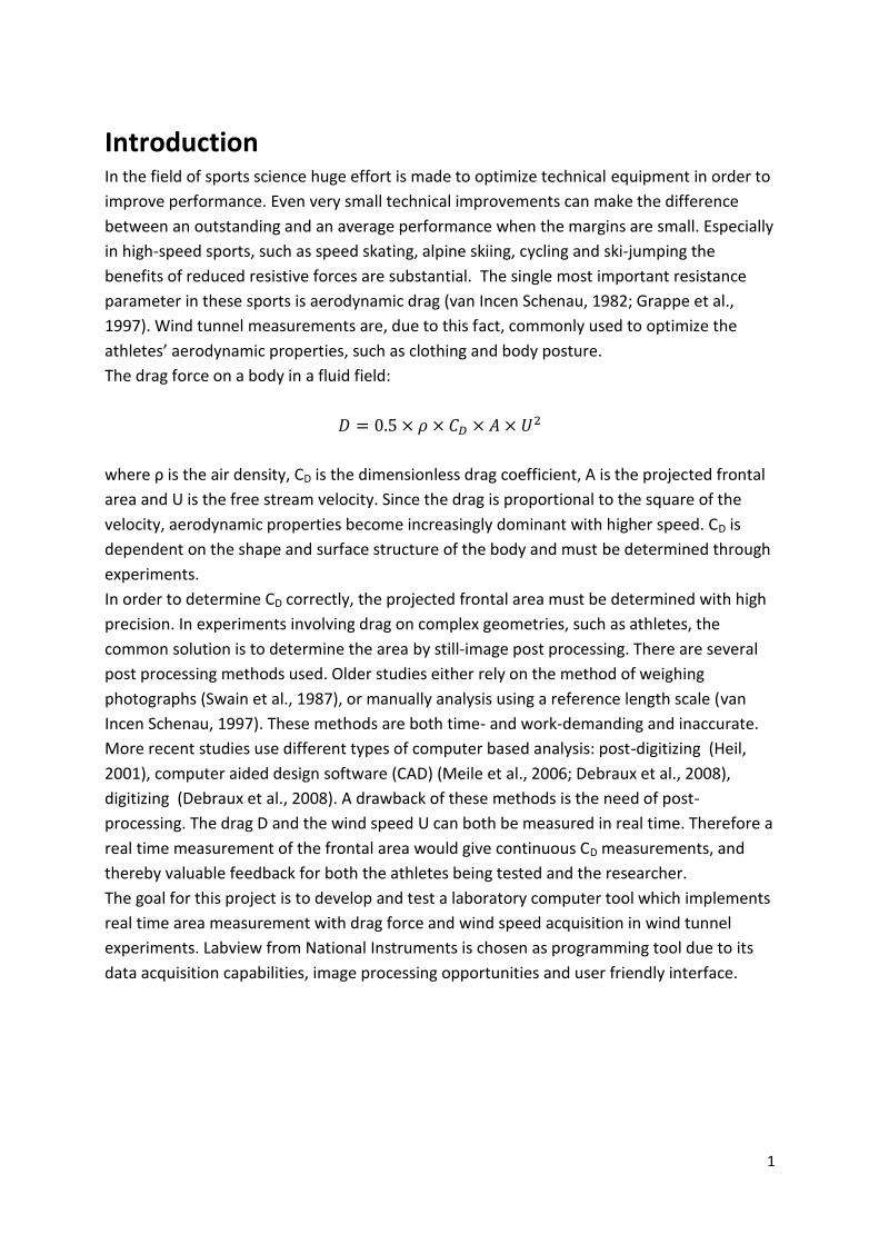
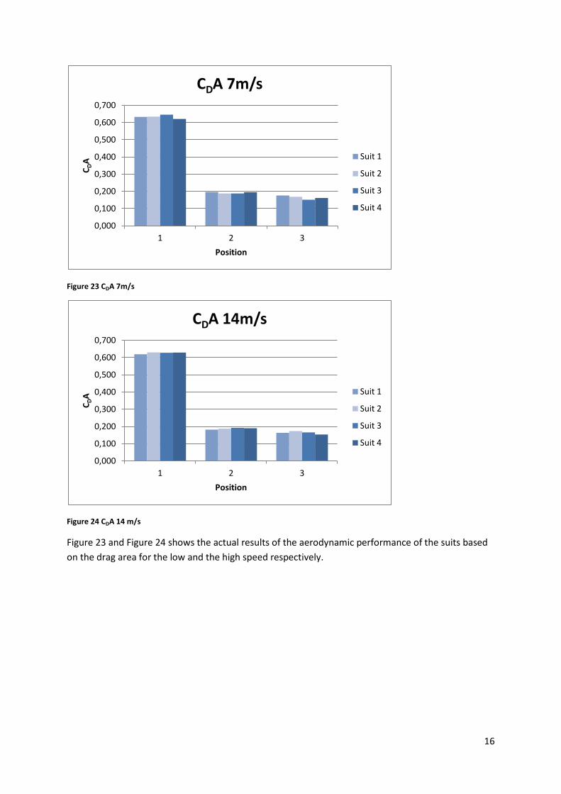
Figure 23 CDA 7m/s

Figure 24 CDA 14 m/s

Figure 23 and Figure 24 shows the actual results of the aerodynamic performance of the suits based

on the drag area for the low and the high speed respectively.

0,000

0,100

0,200

0,300

0,400

0,500

0,600

0,700

1 2 3

CDA

Position

CDA 7m/s

Suit 1

Suit 2

Suit 3

Suit 4

0,000

0,100

0,200

0,300

0,400

0,500

0,600

0,700

1 2 3

CDA

Position

CDA 14m/s

Suit 1

Suit 2

Suit 3

Suit 4

17

Discussion The test results clearly show that the LabVIEW program area measurements are strongly dependent

on lightning conditions and the reflective properties of the suit. The red suit analysed in Figure 14

(suit 2) is bright and reflects more light than the background to the camera lens. Still some parts of

the suit is not sufficient illuminated, especially around the thighs and the inside of the arms the

lightning fails somewhat. This is probably because of the poor light setup in the test. The two halogen

lamps mounted on the sides near the roof would give shades on the inside of the arms and under the

crotch with insufficient lightning from the floor and the roof. The test setup only had two 60W lamps

on the floor and no light from the roof. This will affect the measurement in a negative manner. It’s

also considerable noise in the image, especially near the floor. This is probably caused by the poor

light setup and a reflective floor. The reflective stripe in the upright picture is caused by a plate in the

roof and the spots by the neck are caused by electric sockets in the roof. This could easily be

eliminated. The noise around the outlines of the body is mostly due to a reflective steel plate in the

inlet of the wind tunnel which could be removed if necessary. The conclusion that can be drawn from

these images is that if the removable reflective sources in the background are eliminated and the

lightning setup is improved the program will be able to capture a sharp silhouette with little noise

and thereby a better estimate of the projected area. The green and the blue suit (suit 1 and 3)

perform much like the red suit in the test. Considering the black suit in Figure 15 (suit 4) the

conclusion is somewhat different. The shiny, dark black fabric reflects little light except for the direct

reflections from the lamps. The result is a more random reflection from those parts of the suit. Also

here we see some shades on the inside of the legs in the two lower positions. Overall this kind of

dark shiny fabric doesn’t seem suitable for this method of area measurement.

Considering the consistency of the measurements the results is far better. As seen in Figure 16,

Figure 17 and Figure 18 the deviation from the reference method is fairly constant for all suits except

for suit 4 as expected. The area measured by the LabVIEW program is for suit 1 through 3 higher than

the reference method for all three positions. The excess area is most probably mainly related to

background noise. As expected the area of suit 4 is much and not consistent with the other suits.

Figure 19 shows the deviation from the reference method in percentage of the reference area. It’s

observed that the measurements of suit 1 through 3 is fairly consistent within each position, but

varies between the positions. The variation can also be explained by the background reflections.

Position 1 has a higher gross area of measurement and would therefore contain more reflections as

seen in Figure 14. Position 2 and 3 has the same gross area, but position 3 seem to reveal some more

background reflections from the tunnel inlet because of the lower position, and this could explain the

higher error in position 3. Figure 20 shows how the measured area varies for all suits varies between

the measurements for the upright position. Again the results for suit 1 through 3 don’t vary much

more than can be expected for a human model and the results are almost aligned. In Figure 21 the

variation is shown for all suits in all position as measured in the second session (5 samples). The

results indicates the same trend as shown in Figure 20, fairly consistent results for suit 1 through 3,

while the measurements of suit 4 is both lower than the other suits and more scattered. It can also

be observed that suit 1 is in the lower end of the measurement scale of suit 1 through 3, especially in

the upright position. This suit is also made in a dark fabric and is less reflective than suit 2 and 3. This

would result in a lower outline contrast especially in the undesirable shadow areas.

18

Figure 22 is based the speed and drag measurements acquired simultaneously with the area

measurements and shows the drag area CDA as a function of the area for the three positions. The

lines in the resulting graph should have approximately the same slope and be nearly aligned. Again

suit 2 and 3 give the most accurate results while suit 4 is very inaccurate.

Figure 23 and Figure 24 shows the actual performance of the four suits based on the drag and speed

acquisition. These results are independent of the area, and show us that the suits that have the

lowest drag area in the high speed test also has the highest drag area in the low speed test. This can

be explained by the increasing influence of turbulent wake effects over skin friction with increasing

speed.

Conclusion From the result presented in this report and the experiences made during the testing of the program

it can be concluded that the programs basic functions work as intended and that the programs data

acquisition and sampling functions is a handy tool in wind tunnel experiments. The measurements

are also stable and consistent for fairly reflective surfaces. However it can be stated that the accuracy

of the area measurement, which is the main functionality of the program, is highly dependent on

accurate lightning and a non-reflective background. Also the reflective properties of the measured

object have influence on the result. The surface of the object has to have higher reflection than the

nearby background in at least one colour plane. For this purpose it would be very beneficial for the

accuracy if the interior of the tunnel was mat black. It was shown that a dark black surface like suit 4

could not be measured correctly because of its more random reflections.

Like it is now the program does not produce accurate area measurements in this wind tunnel with

this setup, but with certain improvements it’s believed that the accuracy could increase. The lighting

setup should at least have four powerful halogen lamps and have light falling from four different

angels to produce an accurate illumination of the object. This would reduce shadows and background

noise due to a sharper contrast. The highly reflective objects in the background should also be

eliminated. It must be considered that these measurements was performed using a simple USB

webcam with low resolution. The measurement accuracy would certainly benefit from a better

optical devise with less noise and higher resolution. The program is able to connect to any USB

interface live caption camera device, and can easily be manipulated to measure the light portion of

the area instead of the dark to be applied in other environments.

19

Recommendations for improvements I would recommend that some further work is done on the experimental setup before the program

can be used in science.

Better lightning arrangement/illumination of the object. I would recommend at least four

powerful light sources: one from each side, one from the floor and one from the roof behind

the object.

Elimination of background reflections. Ideally a mat dark background is preferred. At least

there should be no white or metallic reflective surfaces behind the object.

Large scale calibration. The calibration sheet should be black and white with two high

contrast edges and preferably in the scale of the test object. A possible calibration program

improvement could be to do the calibration from a known area.

Possibility to implement an area offset value that compensates for the excess area.

Better camera equipment. A digital video camera with USB live view compatibility would

provide a higher resolution and better optics.

20

References

van Incen Schenau, G.J. (1982): The influence of air friction in speed skating

Grappe, F., Candau, R., Belli, A. and Rouillon, J.D. (1997): Aerodynamic drag in field

cycling with special reference to the Obree’s position

Swain, D.P., Coast, J.R., Clifford, P.S., Milliken, M.C. and Stray-Gundersen, J. (1987):

Influence of body size on oxygen consumption during bicycling

Heil, D.P. (2001): Body mass scaling of frontal area in competitive cyclists

Meile, W., Reisenberger, E., Mayer, M., Schmölzer, B., Müller, W. and Brenn, G.

(2006): Aerodynamics of ski jumping: experiments and CFD simulations

Debraux, P., Bertucci, W., Manolova, A.V., Rogier, S. And Lodini, A (2008): New

Method to Estimate the Cycling Frontal Area

(16.12.09) History – National Instruments, http://www.ni.com/company/history.htm

(16.12.09) NI LabVIEW - The Software That Powers Virtual Instrumentation - National

Instruments, http://www.ni.com/labview/

(16.12.09) What Is Data Acquisition?- National Instruments,

http://www.ni.com/dataacquisition/whatis.htm