Measurement of trace components in aqueoussolutions with near and mid infrared

Fourier transform spectroscopy

Peter Snoer Jensen

Lund Reports on Atomic PhysicsLRAP-299

Doctoral ThesisDepartment of Physics

Lund Institute of TechnologyMarch 2003

This thesis was typeset by the author on an Intel based computer running theGnu/Linux operating system with the command:

cat thesis.ms|soelim|refer|tbl|pic|eqn|groff -ms -P-g >thesis.ps

and afterwards transformed from postscript format into pdf format with pstopdf.

Vi, ed and ghostview were used for editing and viewing the thesis. Data wereprocessed using ANSI C programs based on routines from Numerical Recipes inC by Press et al. and compiled with the GCC compiler. sh scripts, sed and AWKfilters were used to automate complicated calculations. Visualization and graphswere prepared using Gnuplot. The scientific papers were written using the TEXsystem. The author warmly recommends these tools.

Copyright © 2003 Peter Snoer JensenPrinted by Pittney Bowes Management Services, DKMarch 2003

Lund Reports on Atomic Physics, LRAP-299ISSN 0281-2162LUTFD2(TFAF-1052)/1-54(2003)ISBN 91-628-5587-5

Contents

Abstract . . . . . . . . . . . . . . . . . . . . . . 2List of papers . . . . . . . . . . . . . . . . . . . . 31. Introduction . . . . . . . . . . . . . . . . . . . . 42. Infrared Spectroscopy . . . . . . . . . . . . . . . . 73. Fourier transform infrared spectroscopy . . . . . . . . . . . 94. Dual-beam Fourier transform infrared spectroscopy . . . . . . . 235. Quantitative analysis . . . . . . . . . . . . . . . . . 286. Chemometric calibration techniques . . . . . . . . . . . . 307. The near and mid infrared absorption spectrum of water . . . . . . 388. Trace component quantification in aqueous solutions . . . . . . . 409. Haemodialysis treatment . . . . . . . . . . . . . . . . 42Acknowledgements . . . . . . . . . . . . . . . . . . 45Summary of papers . . . . . . . . . . . . . . . . . . 46References . . . . . . . . . . . . . . . . . . . . . 48

2

Abstract

This thesis treats various aspects of the measurement of trace components inaqueous solutions with Fourier transform infrared spectroscopy. This techniquehas several applications from such diverse fields as dairy industry and biomedicaloptics. The use of infrared spectroscopy for trace component quantification ismade difficult by the large absorption of water which dominates the spectrum.The signals from the trace components are small in comparison and must bedetected under circumstances where the water spectrum determines both instru-ment configuration and usable wav enumber regions. In addition the absorption ofwater may be changed by the presence of other components in the solution or byvariations in temperature. The papers, upon which this thesis is based are con-cerned with several aspects relating to this problem. The influence of the waterabsorption spectrum and the configuration of spectrometers are discussed. Onepublication treats the problem of selection of optimal transmission cell pathlengthfor measurement of trace components in aqueous solutions. Another publicationpresents a dual-beam, optical null, Fourier transform spectrometer for measure-ments of trace components in the near infrared spectral range that offers animprovement compared to traditional Fourier transform spectrometers. A thirdpublication presents measurements of the temperature induced variations of theabsorption spectrum of water and of aqueous solutions of glucose. In addition,two specific applications, both concerning the measurement of trace componentsin spent dialysate, are demonstrated. One manuscript describes the application ofthe the dual-beam spectrometer to measure real-time, on-line concentrations ofurea in spent dialysate during treatment of patients. Finally, a manuscript demon-strates the feasability of simultaneous measurement of urea, phosphate, and glu-cose concentrations in spent dialysate with mid infrared transmission spec-troscopy.

3

List of Papers

This thesis is based upon the following papers:

I Peter Snoer Jensen and Jimmy Bak, ‘‘Measurements of Urea and Glucosein Aqueous Solutions with Dual-Beam Near-Infrared Fourier-TransformSpectroscopy’’ Appl. Spectrosc. 56, 12, pp. 1593-1599 (2002)© 2002 Society for Applied SpectroscopyReprinted with permission.

II Peter Snoer Jensen and Jimmy Bak, ‘‘Near-Infrared Transmission Spec-troscopy of Aqueous Solutions: The Influence of Optical Pathlength onSignal-To-Noise Ratio’’, Appl. Spectrosc. 56, 12, pp. 1600-1606 (2002)© 2002 Society for Applied SpectroscopyReprinted with permission.

III Peter Snoer Jensen, Jimmy Bak, and Stefan Andersson-Engels, ‘‘TheInfluence of Temperature on Water and Aqueous Glucose AbsorptionSpectra in the Near- and Mid-Infrared Regions at Physiologically RelevantTemperatures’’ Appl. Spectrosc. 57, 1, pp. 28-36 (2003)© 2003 Society for Applied SpectroscopyReprinted with permission.

IV Peter Snoer Jensen, Jimmy Bak, Søren Ladefoged, and Stefan Andersson-Engels, ‘‘On-line monitoring of urea concentration in dialysate with dual-beam Fourier transform near infrared spectroscopy’’ Manuscrip submittedto J. Biomed. Opt.

V Peter Snoer Jensen, Jimmy Bak, Søren Ladefoged, and Stefan Andersson-Engels ‘‘Determination of urea, glucose, and phosphate in dialysate withFourier transform infrared spectroscopy’’ Manuscript submitted to Spec-trochim. Acta. Part A.

Additional material

Poster presentation at the Photonics West SPIE conference 2002 in San Jose CA:Peter Snoer Jensen, Jimmy Bak, Peter E. Andersen, and Stefan Andersson-Engels‘‘Fourier Transform Infrared Spectroscopy of Aqueous Solutions using OpticalSubtraction’’, Proc. SPIE, 4624, 2002 pp. 150-159.

Oral presentation at the Pittsburgh conference 2002 in New Orleans LA: PeterSnoer Jensen and Jimmy Bak, ´´Optical Subtraction Fourier Transform NearInfrared Spectroscopy on Aqueous Solutions’’.

Oral presentation at the Pittsburgh conference 2003 in Orlando FL: Peter SnoerJensen, Jimmy Bak, Søren Ladefoged and Stefan Andersson-Engels, ´´On-linemeasurement of trace components in dialysate with dual-beam FT-IR spec-troscopy’’. Accepted.

4

1. Introduction

Water is the biological solvent. Indeed, life itself is not possible without it.1 Thismay be explained by the abnormally large dielectric constant of water whichgives it a striking ability to dissolve ionic substances.2 Determination of tracecomponents in aqueous solutions is desirable in many div erse applications suchas biomedical diagnostics, dairy industry and waste water analysis. All of theseapplications demand increasing accuracy and reliability, faster answers, simplesample handling and, if possible, non-invasive and non-destructive measurement.The usual chemical analysis does in many cases provide high accuracy and relia-bility but fails to satisfy the other demands.

Methods based on infrared spectroscopy has the potential to satisfy the demandsthat chemical analysis does not. Infrared spectroscopy probes the vibrations ofthe functional groups of molecules by letting infrared light interact with the sam-ple under investigation. This is a non-destructive, and possibly non-invasive,method which is, in principle, capable of identifying and quantifying organicmolecules. Each organic molecule has a unique infrared spectrum, and thestrength of this spectrum is proportional to the concentration of the molecule.This means that simultaneous determination of several trace components fromone spectrum is feasible provided that the spectra are sufficiently different in thespectral regions that are accessible. Unfortunately, the water in aqueous solutionsabsorbs strongly in the infrared spectral region because of its high concentration.The signals of interest from the trace components are small in comparison andmust be extracted from this strong and varying background.

This thesis treats some important aspects of this problem which relates to the fun-damental properties of water itself and to the instrumentation used for infraredspectroscopy of aqueous solutions. This thesis is based on work carried out atRisø National Laboratory, Optics and Fluid Dynamics Department, Denmark. Ithas been largely experimental and has aimed to produce results of general utilityand to take advantage of these results in specialized cases as well. This thesisconsists of five original scientific papers and the present summary that describesthe field to which these papers contribute. This summary makes no attempt tocompleteness; references to the literature are provided for that purpose. Materialcontained in the original scientific papers is only minimally duplicated here.

Historically, mid infrared spectroscopy has been used primarily for identificationof pure substances in organic chemistry. The arrival of minicomputers, the HeNegas laser, and the fast Fourier transform in the 1960’s made the Fourier transforminfrared (FT-IR) spectrometer practical. It became the instrument of choicebecause it improves signal-to-noise ratio by orders of magnitude compared to a

5

grating instrument.† At about the same time multivariate methods for analysis ofspectral data with many independent overlapping variations found applications inthe chemical field. These methods have made quantitative analysis practical insituations where simple measurements of peak heights to determine concentra-tions are impossible because the peaks are masked by other variations in thespectra that are comparable or much larger. Since then improvements in instru-mentation, and the huge progress in data processing capability caused by theincreased capability of electronic computers and resulting progress in the devel-opment of algorithms for numerical analysis has had tremendous impact. Appli-cations of mid infrared spectroscopy for quantitative analysis of substances hashad large success in gas analysis where spectral lines are sharp and isolated, andthe background transparent. The use of near infrared spectroscopy has emergedsince the 1970’s as a technique for on-line monitoring and process control that isnow widely used.3 Within the biomedical field, vibrational spectroscopy isemerging as a potential diagnostic tool with many div erse applications.4 Theincreasingly prevalent disease diabetes mellitus has created a demand for contin-uous non-invasive monitoring of blood glucose concentration. Therefore, meth-ods to do so based on a variety of techniques, including near and mid infraredspectroscopy, has been sought intensively in latter years.5-15 The arrival of FT-IRmicroscopes for multi-spectral imaging of tissue has spawned considerableresearch to characterize cancer from infrared spectra in the hope that pathologistsmay be given an objective tool for diagnosis.16-19

In the research related to the application of infrared spectroscopy for the mea-surement of trace components in aqueous solutions, much effort has gone into thedevelopment of multivariate techniques and the application of these techniqueson model systems. Most of the work presented in this thesis investigates thepossibility of obtaining the best possible measurements in a given spectral regionby consideration of the limitations imposed by the water and the used instrumen-tation. The motivation for this approach may be found in the huge success of themultivariate methods that have reached a level where only marginal furtherimprovements may be expected. Another motivation may be found in theprevalent optimization methods within this field that are frequently based onresults from chemometric calibration experiments. The conclusions reachedfrom such experiments are frequently disregarding the influence of the waterabsorption spectrum or conditions imposed by the instrumentation. Rather, dataare regarded as isolated quantities with the result that misleading conclusions areformed. The standard Fourier transform spectrometer is almost exclusively usedfor accurate measurements of spectra of aqueous solutions. Part of this thesis

† This improvement is a result of the so-called Fellget, Jaquinot, Connes, and reso-lution advantages that are discussed in section 3.3.

6

investigates the possibility of improving this instrument by operating it in a dual-beam, optical null mode. Within the biomedical field, the determination of tracecomponents in spent dialysate from treatment of patients with renal defects is ofdiagnostic value. This thesis presents measurements of three key components,namely urea, glucose, and phosphate, with the purpose of quantifying thesemolecules on-line during the treatment of patients and thereby eliminate the needfor a traditional analytical chemical analysis. On-line quantification of urea con-centrations has been carried out during the treatment of patients with the dual-beam, optical null, instrument.

The present summary will briefly explain the fundamental principles of infraredspectroscopy. Then follows a description of the standard Fourier transform spec-trometer. The advantages, limitations and applications of dual-beam, optical sub-traction Fourier transform spectroscopy is then described. Having presented thefundamental physics and instrumentation, a description of the principles of quan-titative analysis, and multivariate analysis is given. After this discussion of themethodology and techniques found in this field, a discussion of the the absorptionproperties of water is presented. A discussion of the measurement of trace com-ponents in aqueous solutions follows. Lastly, a general description of renal dis-eases and the treatment of patients by haemodialysis is given. The importance ofmonitoring the treatment is stressed and the motivation for applying FT-IR spec-troscopy to do so is giv en.

7

2. Infrared Spectroscopy

This chapter gives a brief overview of the most basic concepts of infrared spec-troscopy. Standard references are the books by Colthup, Daly, and Wiberley,20

and Pavia, Lampman, and Kriz.21

In a simple model of a molecule, one finds that the bond strength in moleculesand their mass determines the resonant frequencies at which vibrations are exitedand light is absorbed. In the simplest description, two atoms in a bond areregarded as a simple harmonic oscillator with resonant frequency in wav enumberunits†

ν =1

2π c √ K /µ (2.1)

where K is the force constant, µ = m1m2/(m1 + m2) is the reduced mass of thetwo molecules with masses m1 and m2, respectively. Typical atomic masses are1, 12, and 16 atomic mass units (exemplified by the H, C and O atom, respec-tively) and bond strengths are 8. 5, 4. 5 and 16 N/cm (exemplified by the CHbond, the OH bond in H2O and the CO bond in CO2, respectively)22 Therefore,resonant frequencies lies in the infrared part of the electromagnetic spectrumfrom 4000 − 500 cm−1 (2. 5 − 12 µm). Stretching, bending and even more compli-cated vibrational modes, including several atoms in a molecule, may be excited.Stretching vibrations have large force constants and exists in the high wav enum-ber region, whereas bending vibrations have comparatively smaller force con-stants and exists in the low wav enumber regions. In addition, overtone and com-bination bands may be excited because of anharmonicity of the vibrations, suchthat light with higher frequencies may exite these vibrations. For a vibration tobe infrared active, it must cause a change in the dipole moment of the molecule.20

Therefore, vibrations around a center of symmetry are not infrared active.‡ Formolecules in the gas state, fine structure of absorption bands arise from the differ-ent rotational states. Molecules in the liquid state interact so frequently by colli-sions that absorption bands are broadened. Molecules in the solid state are lockedsuch that peaks are more distinct than in the liquid state. The infrared spectrumof a given molecule provides information about the functional groups present init and may be used to identify the molecule. The concentration of a givenmolecule may also be determined, see chapter 5. Interestingly, the thermal radia-tion from matter at temperatures from room temperature to 800 K has it’s maxi-mum between 2200 and 500 cm−1. The maximum moves tow ards higher fre-quencies as the temperature is increased. Therefore, infrared spectroscopy is also

† The wav enumber unit cm−1 is commonly used in infrared spectroscopy. It is thefrequency of the radiation divided by the speed of light c. To convert wav enumbersin cm−1 to wav elength in µm divide 104 with the wav enumber.

‡ In contrast, the Raman effect, which is inelastic scattering of radiation, requires achange in polarizability and therefore a change in the induced dipole moment.

8

used for measurements of temperature, determination of spectral emissivity, andremote sensing.

9

3. Fourier transform infrared spectroscopy

Fourier transform infrared (FT-IR) spectroscopy is today the standard techniquefor quantitative measurements of infrared spectra. The key concepts of this tech-nique are presented in this chapter as an introduction to the field. The purpose isto supply the reader with a basic understanding of the technique and present it’spossibilities and limitations with a special emphasis on the applications relatingto measurements of aqueous solutions. Fourier transform infrared spectroscopyis a vast subject. The short description presented here is based on material fromthe texts by Griffiths and de Haseth23 and Hirschfeld24 to which the reader is ref-ered for further details.

3.1. Basic working principle

The Fourier transform infrared spectrometer is basically a Michelson interferom-eter with a broadband light source, a detector, and an accurate control of the mir-ror displacement. A schematic drawing is shown in Fig. 3.1. The intensities ofthe beams for a monochromatic ligth source with unit intensity, the optical path-length difference, φ , and the beamsplitter reflectance and transmittance coeffi-cents R and T are illustrated in the figure.† The mirror displacement is con-trolled by measuring the zero-crossings of the interference signal from a HeNelaser also passing through a Michelson interferometer. Sev eral different practicalrealizations of this instrument are possible and commercially available. The onewe have used is implemented with corner-cubes instead of flat mirrors as shownin Fig. 3.2. Again the intensities of the beams are illustrated for a monochromaticlight source of unit intensity. The arrangement with corner-cubes has two advan-tages. Firstly, the corner-cubes reflect light 180° regardless of the angle of theincoming light making the configuration immune to tilts of the mirror. Secondly,the corner-cubes separate the incoming and outcoming ray, making the use oftwo inputs and two outputs of the interferometer practical.

The FT-IR spectrometer measures an interferogram hn, which is an array of dis-cretely measured points, containing the AC variation of the intensity at the detec-tor as a function of the displacement of the movable mirror. This interferogram.is converted to an intensity spectrum of the light by Fourier transformation asexplained in section 3.2.

Because of the high accuracy of the mirror position, determined by the interfer-ence signal of the HeNe laser, multiple scans may be co-added such that a linearav eraging of the signal may be carried out. In principle, this allows improvementof the signal-to-noise ratio with the square root of the number of scans. Themaximum displacement of the movable mirror determines the spectral resolution

† The optical pathlength difference is two times the mirror displacement.

10

Lightsource

1 − 2RT (1 + cos φ )

1

Beam-splitter

Movablemirror

Fixed mirror

2RT (1 + cos φ )

Detector

Sample

φ

Figure 3.1: Schematic drawing of Fourier transform infrared spectrometer. Theintensity of the beams are sketched for a monochromatic light source of unitintensity.

of the spectrometer.

3.2. Calculation of single-beam spectrum

For an ideal beamsplitter with no absorption, equal transmittance and reflectancecoefficients R = T = 0. 5, and a monochromatic light source with intensity p1 atwavenumber ν , the intensity P1, measured at the detector as function of the phaseshift φ = 2πν γ at an optical pathlength difference of γ is given by

P1 = 0. 5p1(1 + cos φ ). (3.1)

The AC variation of this signal is known as the interferogram. It is a cosine func-tion with period determined by the wav enumber of the incoming light. For abroad-band light source, the measured signal is a superposition of the cosinefunctions belonging to each wav enumber. The relation bewteen the interferogramand the spectrum of the light source is therefore ideally a cosine transform. Inpractice, the interferogram is never completely symmetric and it therefore alsocontains sine components.

The measured interferograms in this thesis have all been double-sided, that issymmetrical around the zero pathlength difference point. An example interfero-gram is shown in Fig. 3.3. They hav e been converted into single-beam intensityspectra as shown in the flowchart Fig. 3.4. First the mean of the interferogram issubtracted. Then, the interferogram is apodized by multiplication with a window

11

Lightsource

1 Beamsplitter

1 − 2RT (1 + cos φ )

Movablemirror

Fixed mirror

2RT (1 + cos φ )

Detector

Sample

φ

Figure 3.2: Schematic drawing of Fourier transform infrared spectrometer withcorner-cube mirrors. Dashed lines show second input and output. The intensityof the beams are sketched for a monochromatic light source of unit intensity.

function. This apodization function is zero at the endpoints of the interferogramand one in the center. It’s purpose is to make the interferogram zero at the ends,such that discontinuities are avoided. Many different apodization functionsexists.23, 25, 26 They differ in the tradeoff between reduction of sidelobes, and res-olution of the spectrum. The interferogram is then zero-filled by an integerpower of two if a spectrum with artificial higher resolution is desired.† The inter-ferogram is then optionally rearranged by splitting it in two halves and exchang-ing them. This rearrangement is in principle not necessary. It merely shifts thephase by making the interferogram symmetrical around the first array element.The interferogram is then Fourier transformed using the relation

Hn =N−1

k=0Σ hk e2π ikn/N . (3.1)

† The tails of the double sided interferogram is extended with a number of zero’smimicking a spectrum measured with a higher maximum mirror displacement andtherefore a higher spectral resolution. But as the added values are nothing butzero’s, no additional spectral information is obtained. The result is an interpolationin the spectral domain under the assumption that no higher resolution componentsthan those in the measured interferogram are present.26

12

-4

-3

-2

-1

0

1

2

3

4

-0.004 -0.002 0 0.002 0.004

Inte

nsity

/ V

Mirror displacement / cm

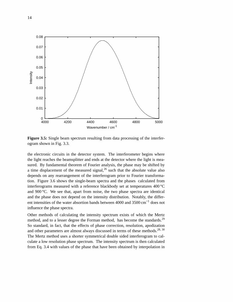
Figure 3.3: Central part of interferogram measured at 32 cm−1 resolution through1 mm of water using a Peltier cooled InAs detector. Short wav elengths has beenremoved by a long wav e pass filter with cutoff at 5000 cm−1. The single beamspectrum resulting from data processing of this interferogram is shown in Fig.3.5.

In practice this is implemented using the fast Fourier transform (FFT)algorithm.26, 27 The inverse relation is given by

hk =1

N

K−1

n=0Σ Hne−2π ikn/N , (3.2)

where Hn is the complex array containing the Fourier transform of hn ThisFourier transform is a function of wav enumber ν . There is no universal agree-ment as to the sign in the exponent of the forward and inverse Fourier transform,nor to the distribution of the normalisation constant 1/N .26 The measured inter-ferogram is real. Consequently, the values at negative frequencies are the com-plex conjugates of their positive counterparts. Therefore, time and storage may bereduced by a factor of two by using a special implementation of the discreteFourier transform.27 The phase spectrum Φ(ν ) is then calculated as

Φ(ν ) = atan(Im(ν )/ Re(ν )), (3.3)

13

where Re(ν ) and Im(ν ) are the real and imaginary parts of Hn, respectively, withindex n corresponding to ν .

IgramSubractMean

Apodize Zero-fill

Re-ArrangeFourier

TransformPhase

SpectrumIntensitySpectrum

Store/ReadPhase

Figure 3.4: Flowchart describing the data processing of interferograms. Dashedboxes are optional.

The calculation takes into account the sign of the nominator and denominator,thereby mapping the angle correctly onto the full unit circle.† From this phasespectrum, the intensity spectrum I (ν ) is calculated as

I (ν ) = Re(ν ) cos Φ(ν ) + Im(ν ) sin Φ(ν ). (3.4)

This procedure has two advantages compared to the nearly equivalent calculationof a power spectrum as

P(ν ) = (Re(ν )2 + Im(ν )2)1/2. (3.5)

In the power spectrum, P(ν ), noise will always give a positive contribution, whilenoise in the intensity spectrum, I (ν ), contributes with both positive and negativevalues.25 The calculation of the intensity spectrum also makes it possible to sub-stitute a phase calculated from another interferogram. This is necessary in dual-beam applications, to be described in chapter 4, where the phase of the dual-beam spectrum is poorly determined because of high nulling ratio, finite resolu-tion, and resulting leakage of information between neighboring points in thespectrum.28 The intensity spectrum resulting from this processing of the interfer-ogram from figure 3.3 is shown in figure 3.5.

Physically, the phase does not depend on the light intensity entering the interfer-ometer. The phase is a wav enumber dependent property of the interferometer and

† The standard function atan2(x,y) in C and FORTRAN is designed for this pur-pose.

14

0

0.01

0.02

0.03

0.04

0.05

0.06

0.07

0.08

4000 4200 4400 4600 4800 5000

Inte

nsity

Wavenumber / cm-1

Figure 3.5: Single beam spectrum resulting from data processing of the interfer-ogram shown in Fig. 3.3.

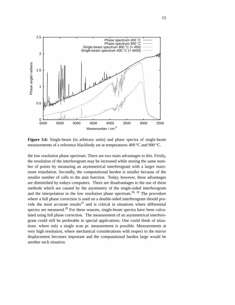
the electronic circuits in the detector system. The interferometer begins wherethe light reaches the beamsplitter and ends at the detector where the light is mea-sured. By fundamental theorem of Fourier analysis, the phase may be shifted bya time displacement of the measured signal,26 such that the absolute value alsodepends on any rearrangement of the interferogram prior to Fourier transforma-tion. Figure 3.6 shows the single-beam spectra and the phases calculated frominterferograms measured with a reference blackbody set at temperatures 400 °Cand 900 °C. We see that, apart from noise, the two phase spectra are identicaland the phase does not depend on the intensity distribution. Notably, the differ-ent intensities of the water absortion bands between 4000 and 3500 cm−1 does notinfluence the phase spectra.

Other methods of calculating the intensity spectrum exists of which the Mertzmethod, and to a lesser degree the Forman method, has become the standards.29

So standard, in fact, that the effects of phase correction, resolution, apodizationand other parameters are almost always discussed in terms of these methods.28, 30

The Mertz method uses a shorter symmetrical double sided interferogram to cal-culate a low resolution phase spectrum. The intensity spectrum is then calculatedfrom Eq. 3.4 with values of the phase that have been obtained by interpolation in

15

0

0.5

1

1.5

2

2.5

25003000350040004500500055006000

Pha

se a

ngle

/ rad

ians

Wavenumber / cm-1

Phase spectrum 400 ˚CPhase spectrum 900 ˚C

Single-beam spectrum 900 ˚C (× 450)Single-beam spectrum 400 ˚C (× 4500)

Figure 3.6: Single-beam (in arbitrary units) and phase spectra of single-beammeasurements of a reference blackbody set at temperatures 400 °C and 900 °C.

the low resolution phase spectrum. There are two main advantages to this. Firstly,the resolution of the interferogram may be increased while storing the same num-ber of points by measuring an asymmetrical interferogram with a larger maxi-mum retardation. Secondly, the computational burden is smaller because of thesmaller number of calls to the atan function. Today, howev er, these advantagesare diminished by todays computers. There are disadvantages to the use of thesemethods which are caused by the asymmetry of the single-sided interferogramand the interpolation in the low resolution phase spectrum.28, 30 The procedurewhere a full phase correction is used on a double-sided interferogram should pro-vide the most accurate results25 and is critical in situations where differentialspectra are measured.28 For these reasons, single-beam spectra have been calcu-lated using full phase correction. The measurement of an asymmetrical interfero-gram could still be preferable in special applications. One could think of situa-tions where only a single scan pr. measurement is possible. Measurements atvery high resolution, where mechanical considerations with respect to the mirrordisplacement becomes important and the computational burden large would beanother such situation.

16

3.3. Advantages over grating instrument

The FT-IR spectrometer has replaced the grating instrument because it possessesa number of advantages. These advantages have been discussed by Hirschfeld,24

Griffiths and de Haseth23 and others. Here follows a short description of theseadvantages and some comments regarding their impact on measurements onaqueous solutions.

In a traditional grating instrument, each spectral point is measured sequentially.In contrast, an FT-IR instrument measures all spectral points simultaneously. Thisresults in an improvement in SNR proportional to √ N where N is the number ofspectral points. This is known as the Fellget advantage. For measurements onaqueous solutions, the spectral range is usually limited to a narrow regionselected by the chosen pathlength of the transmission cell and the spectral resolu-tion is chosen to be low because of the broad absorption found in the liquid state.If we assume a spectral range of 1000 cm−1 with a spectral resolution of 16 cm−1

we have an improvement by roughly a factor of eight compared to a gratinginstrument. A grating instrument with a detector array will also measure all spec-tral points simultaneously and an FT-IR spectrometer will possess no Felgettadvantage over such an instrument.

The absence of a slit in an FT-IR instrument increases it’s light gathering powercompared to a grating instrument. The light gathering power is usually expressedas the product of the allowed solid angle of the incoming beam and it’s cross sec-tional area and is known as the troughput Φ. The ratio of throughputs in the FT-IR and grating case is given by Griffiths and de Haseth as23 as

ΦF

ΦG=

2π AF faν 2

AGhνmax, (3.6)

where index F refers to the FT-IR instrument and G to the grating instrument A isthe area of the mirror / grating, f is the focal length of the grating instrument h isthe slit height and a the grating constant. This advantage is seen to be largest athigh wav enumbers, it is commonly known as the Jaquinot advantage. TheJaquinot advantage is reduced in cases where sensitive cooled detectors areemployed. In these cases, it is commonly necessary to reduce the intensity reach-ing the detector to avoid saturation.

Wa venumber determination is accurate through the fringe determination of theHeNe laser. This not only means that high resolution spectroscopy is possible,but also allows co-addition of spectra such that the signal to noise ratio may beimproved by the square root of the number of scans. This reproducibility of thewavenumber scale is also important when weak absorption on a large backgroundis to be detected. This advantage is known as the Connes advantage.

17

The resolution of an FT-IR spectrometer depends only on the mirror displace-ment which may be accurately determined. The larger the displacement thehigher the spectral resolution. This advantage is of less importance in spec-troscopy of aqueous solutions, where the required spectral resolution is low.

3.4. Limitations of FT-IR spectrometers

The FT-IR spectrometer is an instrument, which is capable of achieving extraor-dinarily high signal-to-noise ratios. Even so, there are disadvantages to this tech-nique that become important when the ultimate performance of these instrumentsrequired. An elaborate discussion of instrumental effects in FT-IR spectroscopyis given by Hirschfeld.24 This includes effects of mirror displacement from sam-pling points, double modulation of radiation, emission from the detector andother effects.

Many instrumental effects become serious because the measurement of anabsorbance spectrum with an FT-IR spectrometer is a two stage process.† First areference spectrum I0(ν ) is measured and then a sample spectrum I (ν ). The tem-poral difference between the two measurements means that the instrumental vari-ations are not necessarily eliminated, and one is left with a signal where one haspayed for stability, by accepting increased noise, without receiving it.‡ Suchinstrumental variations may happen on timescales smaller than the time requiredfor a single scan, such that it is impossible to measure a satisfactory reference.The co-addition of interferograms to reduce noise also means that the temporaldifference between the measurement of sample and reference increases. Sec-ondly, the measurement of a small signal riding on top of a large signal is alwaysundesirable because small changes in the large signal may be comparable to thesmall signal one measures. Thirdly, the finite dynamic range of the analog-to-digital converter means that the digitization of a signal with a large dynamicrange of which the relevant information is stored in only very few bits is undesir-able. In the case where detector noise is sufficiently low and the intensity reach-ing the detector sufficiently high, the large dynamic range may even result in asituation where signal-averaging by co-addition of sequential scans does notimprove signal-to-noise ratio because the noise is smaller than the distancebetween two bits on the analog-to-digital converter. In this case one speaks ofdigitization noise.23 § In on-line applications, the ideal optical sensor is small

† Grating instruments are usually dual-beam instruments with a chopper that alter-nates a beam through a sample and reference such that a modulated signal is mea-sured at the detector. In this fashion, the spectrometer measures the transmittanceof the sample directly.

‡ When analysis is based on single-beam spectra, such variations are not evensought to be compensated in the measurement process.

§ The application of dual-beam FT-IR spectroscopy attempts to remove these prob-

18

with no moving parts, cheap and simple. In contrast, the FT-IR spectrometer islarge, expensive and complicated.

3.5. Sources in IR and NIR

The most commonly used light source used in the mid infrared region is a SiCglobar. This is a rod, heated to a temperature of about 800 °C by a current passingthrough it, which emits thermal radiation with a maximum intensity at approxi-mately 2100 cm−1. In the near infrared region, quartz halogen tungsten filamentlamps, are usually employed. They hav e a temperature of about 2500 °C provid-ing maximum intensity at 5500 cm−1. The absorption of quartz in the midinfrared region prevents application of this light source in that spectral region.

3.6. Detectors in IR and NIR

The standard detector in most FT-IR instruments is the deuterated triglycine sul-phate (DTGS) detector. This is a thermal detector, a so-called pyroelectricbolometer, that consists of a ferroelectric crystal which has a Curie point close toroom temperature. The crystal therefore exhibits large changes in electricalpolarizability when exposed to modulated radiation. By placing electrodes onthe crystal faces, the crystal acts as a capacitor across which an AC voltage maybe measured. This detector is very linear, stable, and has a wide spectral rangeof operation.

Semiconductor based quantum detectors are used when increased sensitivity andlow noise is required. In the mid infrared spectral region, the mercury cadmiumtelluride (MCT) detector is almost exclusively used. This detector usuallyrequires cooling by liquid N2. In the near infrared spectral region InSb and InASdetectors are employed. These detectors may be liquid N2 or Peltier Cooled.Compared with the DTGS detector, these detectors have lower noise, higher sen-sitivity, but a narrower spectral range of operation. The levels of intensity theymay be exposed to is far lower than the ones the DTGS accept. The MCT detec-tor in particular has a non-linear behavior when exposed to too high levels ofintensity.

The difference in linearity between the mid infrared MCT detector and the nearinfrared InSb and InAs detectors may be understood from the structure of thesedetectors. These detectors are constructed to be sensitive to different energy lev-els of radiation. In a semi-conductor structure with a conduction band separatedfrom a valence band by a band-gap, a current can be measured when free electronare created in the conduction band by absorption of photons with energies greater

lems related to dynamic rang by a simultaneous measuerent of the differencebetween sample and reference. The technique is described in chapter 4.

19

than the band-gap. A mid infrared detector has a small band-gap as it is requiredto detect radiation with low energies and thermal excitation creates a consider-able number of electrons in the conduction band, even when the detector iscooled. The reservoir of electrons that may be excited by the incoming IR radia-tion is therefore small. This is illustrated in figure 3.7. With too much light inten-sity reaching the detector, the reservoir is dried out and the detector saturates.

Smallbandgap

Conduction band

Valence band

Zero energy

Many thermal electrons

Small electron reservoir

Radiation excited electrons

Thermally exited electrons

Figure 3.7: Bandgap properties of mid infrared quantum detectors.

A near infrared detector is required to detect much higher energies and, conse-quently, it has a much larger band-gap. For this reason, thermal excitation doesnot create as many electrons in the conduction band. A higher incident flux ofradiation is therefore permissible before saturation sets in. This is illustrated infigure 3.8. The use of dual-beam techniques where the intensity reaching thedetector is twice as high as in the single-beam case is therefore much more lim-ited by the MCT detector in the mid infrared region than by the InAs detector inthe near infrared region. A thorough discussion of infrared detectors is given byKinch.31

3.7. Infrared windows

The window materials used as in FT-IR spectrometers and sample accessoriesmust be transparent to infrared radiation. The most common infrared windowsare salts that are hygroscopic and therefore ill suited for use in connection withaqueous solutions. Most beamsplitters consists of a base of such a material with acoating and FT-IR spectrometers are therefore either sealed, with a dessicatingmaterial within, or purged with dry air, free of water and carbon dioxide. Thesetwo gasses have intense infrared absorption bands and the purge also has the

20

Largebandgap

Conduction band

Valence band

Zero energy

Few thermal electrons

Large electron reservoir

Radiation excited electrons

Thermally exited electrons

Figure 3.8: Bandgap properties of near infrared quantum detectors.

purpose of reducing the concentration of these two gases. The most commonlyused window material for measurements on aqueous solutions is CaF2 which isonly very weakly dissolved by water and has an index of refraction which is closeto that of water. Another commonly used material is ZnSe which has a higherindex of refraction but is soft. In the near infrared spectral range, quartz and sap-phire windows may be employed. They hav e the advantage of being hard andchemically inert. A table of infrared materials is shown in Table 3.1.

Material Spectral range Refractive index Water solubilitycm−1 at 1000 cm−1 g/100g

KBr 48800 − 345 1.52 53.5NaCl 52600 − 457 1.49 35.7CaF2 79500 − 1111 1.39 0.0016ZnSe 15000 − 461 2.4 insol.Sapphire 40000 − 1608 2.6 insol.Suprasil 300® 57142 − 2857 2.5 insol.Diamond 30000 − 30 2.4 insol.

Table 3.1: Properties of infrared window materials. The spectral range is givenfor a window thickness of 1 mm, except for Suprasil, where the thickness is10 mm. Data from Pike Technologies, Madison WI, USA, Catalog 2001.

21

3.8. Sampling techniques

The measurement of an absorption spectrum of an aqueous solution is mainlycarried out using two different sampling techniques, namely through the applica-tion of a transmission cell or an attenuated total reflection (ATR) cell.32 In thiswork, the use of an ATR cell has been limited to preliminary investigations an noATR spectrum is presented. Even so, the technique is standard, and preferred bymany other groups, so a description of both techniques is given. The transmisioncell consists of two IR transparent windows between which the aqueous solutionis placed. The light ray of the interferometer then passes through the IR windowsand the aqueous solution before reaching the detector. This is illustrated in figure3.9.

Light in Light out

Sample

IR windows

Figure 3.9: Schematic drawing of transmission cell.

Transmission cells are well suited for near infrared spectroscopy of aqueous solu-tions. In this spectral region optimal pathlengths are in the range 0. 5 − 10 mmand consequently much larger than the wav elength of the light. In the midinfrared region, the pathlength is in the range 7 − 50µm which is of the sameorder of magnitude as the wav elength of the light. This means that multiplereflection inside the transmission cell may cause fringe effects in the spectrum inthe mid infrared region, but not in the near infrared region.†

The magnitude of this effect increases with the difference between the index ofrefraction of the sample and of the window material. For an accurate determina-tion of the absolute absorption coefficient of water, it is necessary to correct forthe difference in Fresnel reflection at the interfaces in an empty cell and in awater filled cell because the index of refraction of water is dependent on thewavenumber. Instead, one may measure a reference spectrum of a water filledsample, with pathlength δ , and a sample spectrum with a pathlength of d + δ , to

† This effect is normally used to determine the pathlength of a transmission cell.The pathlength is given by d = (n∆ν )−1 where n is the index of refraction of thesample (normally air), and ∆ν is the period of the fringe pattern in cm−1.

22

obtain the absorbance spectrum of the sample at pathlength d , thereby eliminat-ing the difference in index of refraction at the interfaces.

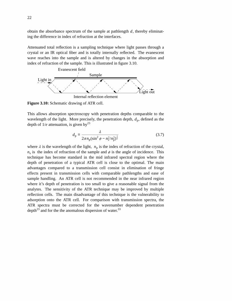
Attenuated total reflection is a sampling technique where light passes through acrystal or an IR optical fiber and is totally internally reflected. The evanescentwave reaches into the sample and is altered by changes in the absorption andindex of refraction of the sample. This is illustrated in figure 3.10.

Light in

Light out

Evanescent fieldSample

Internal reflection element

Figure 3.10: Schematic drawing of ATR cell.

This allows absorption spectroscopy with penetration depths comparable to thewavelength of the light. More precisely, the penetration depth, dp, defined as thedepth of 1/e attenuation, is given by23

dp =λ

2π np(sin2 φ − n2s /n2

p)12

(3.7)

where λ is the wav elength of the light, np is the index of refraction of the crystal,ns is the index of refraction of the sample and φ is the angle of incidence. Thistechnique has become standard in the mid infrared spectral region where thedepth of penetration of a typical ATR cell is close to the optimal. The mainadvantages compared to a transmission cell consist in elimination of fringeeffects present in transmission cells with comparable pathlengths and ease ofsample handling. An ATR cell is not recommended in the near infrared regionwhere it’s depth of penetration is too small to give a reasonable signal from theanalytes. The sensitivity of the ATR technique may be improved by multiplereflection cells. The main disadvantage of this technique is the vulnerability toadsorption onto the ATR cell. For comparison with transmission spectra, theATR spectra must be corrected for the wav enumber dependent penetrationdepth23 and for the the anomalous dispersion of water.33

23

4. Dual-beam Fourier transform infrared spectroscopy

The measurement of weak signals on a strong and varying background is gener-ally considered difficult and the ability of the FT-IR spectrometer to remove acommon background by subtraction of a reference from a sample signal in themeasurement process leaving only their difference has been suggested early byFellget.34 Some nine years thereafter applications of this technique were demon-strated by by Bar-Lev,35 Low and Mark,36 Vanasse,37-39 Griffiths,40 Chan-drasekhar, Genzel, and Kuhl.41-43 The different variants of this technique are allknown as dual-beam FT-IR spectroscopy. Notably, the application of dual-beamFT-IR spectroscopy for measurements on biological samples were suggested byChandrasekhar, Genzel, and Kuhl as early as 1976.41 This chapter will describethe principles of dual-beam FT-IR spectroscopy for the two modes of operationknown as single-input-double-output and double-input-single-output. The advan-tages one seeks to obtain compared to a traditional single-beam mode of opera-tion and the subtle differences between the two modes of operation are described.The limitations and difficulties of the dual-beam FT-IR technique are described.A short list of notable previous applications are given that are followed by amotivation for applying this technique for measurements of aqueous solutions.

In dual-beam FT-IR spectroscopy, the symmetry of the Michelson interferometeris taken advantage of to provide either two inputs or two outputs, or both. This isillustrated in Fig. 4.1. The following presentation closely follows that given byChandrasekhar, Genzel, and Kuhl.41 Assume two monochromatic light sourcesemitting radiation at wav enumber ν with intensities p1 and p2 placed at input 1and input 2, respectively. The intensity at at output 1, P1, will then be

P1 = p12RT (1 + cos φ ) (4.1)+p2[(R + T )2 − 2RT (1 + cos φ ) + 4RT cos Φ cos(φ − Φ)]

+4(p1 p2 RT )12 cos(φ /2) × [R cos(Φ − δ − φ /2) + T cos(Φ + δ − φ /2).

In this expression, φ is the optical phase shift 2πν γ as in section 3.2, Φ is thephase difference between the reflected and transmitted beams on the beamsplitter,δ is the phase difference of the two input beams, and R and T are the reflectanceand transmittance coefficients of the beamsplitter. The corresponding expressionfor the intensity at output 2, P2, will be similar. It may be obtained by exchang-ing p1 and p2, and changing the signs of φ and δ in Eq. 4.1. These two expres-sions may be simpified if we assume that the beamsplitter is ideal such thatR = T = 0. 5 and Φ = π /2. If we further assume that the two inputs are uncorre-lated, the last term in Eq. 4.1 will be rapidly varying and average to zero. Onethen obtains the following expressions for the intensities at the two outputs:

P1 = 0. 5( p1 + p2 + (p1 − p2) cos φ ) (4.2)

24

Input 1Beamsplitter

Output 2

Input 2

Movablemirror

Fixed mirror

Output 1

φ

Figure 4.1: Schematic drawing of Fourier transform infrared spectrometer withcorner-cube mirrors. Dashed lines show second input and output. The possibil-ity of two inputs and two outputs is shown.

and

P2 = 0. 5( p1 + p2 − (p1 − p2) cos φ ). (4.3)

One observes that the sum of the two output intensities is equal to the sum of thetwo input intensities and independent of the optical phase shift, φ . If the twoinputs have identical intensity, both outputs will have zero modulation. If thesecond source intensity is zero, p2 = 0, Eq. 4.2 reduces to Eq. 3.1 as it should.

4.1. Advantages of dual-beam FT-IR spectscopy

The removal of the background common to the sample and reference forces thesignal of interest to emerge from a flat baseline where it is more easily quantified.The dynamic range of the signal is reduced and the full range of the analog-to-digital converter in the spectrometer may be employed to digitize only the signalof interest, excluding the background.† This prevents the spectrometer frombeing limited in performance by digitization noise as described in section 3.4.Most instrumental variations are common to both inputs and should thereforecancel in the measurement process. The optical subtraction happens on a per-point basis in the interferogram with exact synchronicity and is therefore capableof eliminating variations that takes place on timescales smaller than a single scan.

25

4.2. Double-input-single-output mode:

If the two inputs have different intensities, one may measure an interferogram atone of the two outputs which contains only the difference between the twoinputs. This is essentially the method that has been used in papers I and IV.† Inthose papers, light is collected from a single source and two beams are passedthrough each their transmission cell before entering the spectrometer through theinput ports. Let Ts and Tr denote the transmittance of the sample and referencecells, respectively, and let p = p1 = p2 denote the intensity of the commonsource. Equation 4.2 is then modified to

P1 = 0. 5p(Tr + Ts) + (Tr − Ts) cos φ . (4.4)

The direct difference between the transmittances of the two cells is measured asthe AC part of Eq. 4.4. This is known as a double-input-single-output configura-tion.

4.3. Single-input-double-output mode:

If one uses only a single input, p1 and passes the two outputs through a sampleand a reference cell, respectively, before letting them reach a common detector,one speaks of a single-input-double-output configuration. Denoting the transmit-tance of the sample and reference, Tr and Ts, respectively, The intensity at thecombined output is

P1+2 = P1Tr + P2Ts = 0. 5p1(Tr + Ts) + (Tr − Ts) cos φ . (4.5)

Again, one measures only the difference in transmittance between the two sam-ples.

4.4. Differences between the single-input-double-output and the double-input-single-output configurations.

The expressions Eqs. 4.4 and 4.5 look deceptively alike. There are subtle differ-ences although both methods are described as dual-beam, optical null, opticalsubtraction FT-IR spectroscopy. Both methods have in common, that a DC com-ponent of the measured intensity at the detector is two times that found in thenormal single-beam mode of operation of an FT-IR spectrometer. This presentsproblems with saturation of the normally employed MCT detector in the midinfrared spectral region.44 In this spectral region, beamsplitter absorption alsolimits the degree of opticall nulling that may be obtained.23

In the double-input-single-output mode of operation, the eigenradiation of thereference and sample is modulated by the interferometer such that sample and

† For obvious reasons, this is also the mode of operation for dual-beam FT-IRremote sensing applications.

26

reference temperature differences are included in the measurement. The additionof the two beams are simple, because the light in the two beams are uncorrelated,but the technique requires that light with equal intensity and spectral distributionis passed through the sample and reference. The alignment and of the opticalcomponents are facilitated by the placement before the interferometer. The useof two inputs also enable a higher total intensity to be measured compared to theuse of only a single input.

In the single-input-double-output mode of operation, the eigenradiation of thesample and reference remains unmodulated and contributes only with a DC termon the detector which is not measured. In this mode of operation the sample andreference are part of the interferometer and interference problems may arise. Thedetector must be sufficiently large to average out interference fringes resultingfrom this undesired modulation. Another possibility is to measure the light at thetwo outputs with each their detector and add the signals electronically instead.This procedure reduces the interference problems and minimizes the total inten-sity reaching a single detector, but is limited by the requirement that the twodetectors must have identical characteristics. In this case one speaks of electronicsubtraction.

4.5. Earlier applications

The applications have been primarily in the mid infrared region for various mea-surements of weak absorption in a transparent medium with the background to beeliminated consisting of the source intensity distribution. The early applicationof Griffiths, Gomez-Taylor, and Kemeny for the determination of trace compo-nents in gas chromatography is a good examples of a single-input-double-outputexperiment.45, 46 A Later application by Tripp and Hair for the detection ofadsorbed polymer monolayers on mica demonstrates that the double-input-single-output mode of operation may be used with advantage for samples at room tem-perature.47, 48 The work by Beduhn and White demonstrating the feasability ofsingle-input-double-output with electronic subtraction.49 In these cases, The non-linear behavior of the MCT detector has limited the use of this technique,because it becomes necessary to reduce the intensity reaching the MCT detectorwith corresponding decrease in signal-to-noise ratio as a result. As an exampleTripp and Hair reported a nulling ratio of a factor of 50 that only translated intoan improvement in signal to noise ratio of five because of the non-linear behaviorof the MCT detector.

27

4.6. Advantages in the near infrared for measurements on aqoueous solu-tions

As described in section 3.6, near infrared detectors accepts a higher incident fluxbefore they saturate. In addition there is no beamsplitter absorption and theeigenradiation of samples at room temperature is small. The measurement onaqueous solutions in the near infrared spectral range requires only a low resolu-tion. The spectral range may be reduced to a narrow range with no loss of infor-mation because the optical pathlength and the absorption spectrum of water onlyallows a high sighnal-to-noise ratio in a narrow region as described in paper II.The absorption of water also helps to reduce the incident flux on the detector.The optimal transmission pathlenght is long compared to those required in themid infrared region, therefore a couple of transmission cells with equal path-length is easily constructed. We were curious as to wether these advantageswould result in an improvement when the double-input-single-output mode ofoperation were compared with the single-beam mode. Paper I demonstrates, thatone obtains a significant advantage in the combination band 5000 − 4000 cm−1 bymeasuring with a dual-beam instrument instead of a single-beam measurement.Even though the main variations present in both types of measurements, instru-mental variations are eliminated in the dual-beam measurement.

4.7. Differences in computation

As described in section 3.3 the calculation of a dual-beam spectrum from a mea-sured dual-beam interferogram requires the use of a single-beam phase spectrum.Another difference from measurements with a single-beam instrument lies in thecalculation of an absorption spectrum from a sample, I , and a reference I0. Asdescribed in chapter 5, the absorbance, A, is giv en by A = − log10 I /I0. The mea-sured dual-beam spectrum, D, is the difference between the sample and referenceD = I − I0. Therefore, the absorbance may be written with good precision asA = (1/ ln 10) × (D/I0). We hav e assumed that D is much smaller than I and usedthe Taylor expansion for the log function.

28

5. Quantitative analysis

The concepts of quantitative analysis are presented in this chapter. The interestfocuses on the influence of drift and noise as two key factors that determine thesuccess of any quantitative measurement. The advantage of a full spectral mea-surement, as in FT-IR spectroscopy, to distinguish between these two quantitiesand the possibilities for reducing their impact on quantitative measurements arediscussed.

In quantitative analysis, one traditionally measures the absorbance of a substanceto determine a concentration. The absorbance A(ν ), at a given wav enumber ν , isgiven by

A(ν ) = − log10 I (ν )/I0(ν ) (5.1)

where I (ν ) is a measurement of the sample intensity and I0(ν ) is a measurementof the reference intensity. The choice of reference depends on the application. Inmany cases a reference with no sample present is used. In other cases a referenceis chosen which resembles the sample. This issue is disussed in paper II. Mostgrating instruments measure the ratio I (ν )/I0(ν ), known as the transmittance,directly, but the Fourier transform instrument measures the sample and referenceintensity spectra separately. By taking the ratio of I (ν ) and I0(ν ), one creates adimensionless number which ideally eliminates all the dependency on the instru-ment, including spectral intensity distribution of the source and sensitivity of thedetector. This is on condition that the instrument remains constant between themeasurement of sample and reference. Note, that noise is not eliminated and stilldepends on the source and detector. The noise is increased because the relevantsignal is composed of two measurements, each containing noise. The increase innoise pays for elimination of instrumental effects, including drift.

5.1. Beer’s law

Quantitative analysis is based on Beer’s law, which states that the absorbance of asubstance, at a given wav enumber ν , is proportional to the molar concentration cof the substance and the pathlength l:

A(ν ) = ε (ν )cl; (5.2)

where ε (ν ), known as the molar absorptivity, is the wav enumber dependent pro-portionality constant. Beer’s law says that the intensity decays exponentiallywith pathlength and with the concentration of the substance.

Chemometric methods to extract the concentration from a measurement whereseveral components have overlapping signals exists, of which the ones most com-monly applied will be discussed in chapter 6.

29

5.2. Drift, noise, and data pre-treatment

Traditionally drift and influences from instrumental effects have been consideredmore problematic than noise. In applications where small signals are to bedetected, and with the now available methods of data analysis, noise may proveto be more problematic than instrumental effects. If one considers a single pointmeasurement, at a given wav enumber, noise and drift are indistinguishable. Ifone has available a full spectrum, on the other hand, drift and influences of instru-mental variations may be reduced because they hav e a spectral structure that maybe included in the calibration process. Noise, is impossible to remove from a sin-gle spectrum because it is uncorrelated from point to point in the spectrum.

Noise may be reduced by averaging a large number of measurements, but theSNR is proportional to the square root of the number of measurements. Thisstrongly limits this procedure because the measurement time becomes pro-hibitively large.50 In practice it turns out that many FT-IR instruments fail to sig-nal average well beyond a certain point.51 The spectrum may be low-pass filtered,which does in a sense remove noise. But such a procedure is based on a prioriassumptions about the spectrum, which may not be true, and reduces the spectralresolution of the data. In addition, it is doubtful that such a smoothing representsan advantage in a calibration. Smoothing is probably most justified when used asa graphical technique to guide the eye.27 High-pass filtering, including derivation,may remove baseline variations, but such a procedure will also remove anybroad-band variation which is part of the signal of interest. In general, any datapre-treatment which is carried out to remove drift will result in an increased noiseor degraded spectral resolution. Noise therefore ultimately limits the calibration.For this reason, single-beam spectra (or logarithmized single-beam spectra) arealso used today in quantitative analysis. In this case, variations and drift areincluded in the modeling of the data instead of eliminated in the measurementprocess.52 The FT-IR instrument has the advantage over the grating instrument inpossessing a superior signal-to-noise ratio. In contrast, the dual-beam infraredgrating instrument is made to eliminate drift by measuring the transmittancedirectly. The dual-beam, optical null, FT-IR spectrometer also seeks to eliminatedrift in the measurement process, but does so by measuring a difference betweentwo samples instead of a ratio. A dimensionless number is therefore not obtained.

The variability of the sample population also influences the accuracy of any cali-bration. With a large variability in a sample population, many calibration samplesand many independent spectral points will be necessary to maintain stability andaccuracy. The variability of the sample population is usually given as an intrinsicpart of a job, and reducing a population variability then means to exclude certainclasses of samples. This may be necessary, but is seldom desirable.

30

6. Chemometric calibration techniques

In this chapter, various methods for analysis of spectroscopic data are described.These methods have been used in the original scientific papers as availablemethod without a detailed description. This chapter is thus, on purpose, slightlymore extensive than the others providing details not found in the scientificpapers.

In traditional statistics, a large number of measurements of a single quantity, orpaired quantities, are carried out and used to provide the information of interest.There does exist a large class of experiments, to which spectroscopic measure-ments belong, where comparatively few measurements of a large number of inde-pendent quantities are carried out. To take advantage of such data, a reduction ofdimensionality is necessary. This reduction is made possible by the covariancebetween measured variables. Principal component analysis (PCA),53 principalcomponent regression (PCR), and partial least squares regression (PLSR)54 areall methods based on such data reduction schemes. They are, today, the mostcommonly used data analysis methods used in mid and near infrared spec-troscopy for quantitative analysis.

6.1. Principal component analysis

Principal component analysis takes a collection of spectra arranged as a matrix,X, where each row, Xi , is a spectrum, and decomposes this matrix into a productof two other matrices, the score matrix, T, and the transpose of the loadingmatrix, P, and a matrix, E, such that

X = T ⋅ PT + E. (6.1)

The matrix E is zero if the full dimension of P is retained. The advantages of thedecomposition are obtained only when the dimension of the data is reduced. Inthis case, the signal is separated from the noise contained in E as a residual. Thisdecomposition may be viewed as a transformation to another coordinate system,where the new axes, Pi , are the spectra of the variations found in the data set.The new coordinate system is orthonormal and rotated so that the first axis lies inthe centre of the data and minimizes the variance when subtracted from the data.The second axis lies in the center of this new data set where the first axis hasbeen subtracted and so on ... † The new set of axes, P, is known as the loadingsand the coordinates in this new coordinate system, Ti , are known as the scores.

The principal component analysis is identical to a singular value decomposition

† This is a sketch of the NIPALS algorithm, which is commonly used to carry outthe PCA.54 This method may be employed with minor modifications if data pointsare missing. This is not an issue when measuring infrared spectra with a Fouriertransform spectrometer, howev er.

31

(SVD) of the matrix X into the product of an orthonormal matrix, U, a diagonalmatrix, w, and the transpose of an orthonormal square matrix, V:

X = U ⋅ w ⋅ VT (6.2)

In this case, the score matrix, T, is identical to the product of the matrix U andthe diagonal matrix w. Deletion of principal components representing noise, isthen carried out by setting the corresponding small value in the diagonal matrix wto zero. Double precision versions of routines from Numerical Recipes in C27 forsingular value decomposition has been used in this work to carry out the principalcomponent analysis. The difference between the two mathematically equivalentformulations is largely conceptual. PCA stresses the graphical interpretation ofthe data in the transformed coordinate system. The scores (coordinates) may beinterpreted to detect outliers and drift and the loadings (axes) may be interpretedas spectra of the primary variations found in the data. These in turn may be iden-tified with physical or chemical variations.

It is customary to center the data matrix X by subtracting the mean spectrum xbefore carrying out PCA. In some applications the data matrix is scaled by divi-sion with the standard deviation spectrum, s. We hav e not done that in this work.

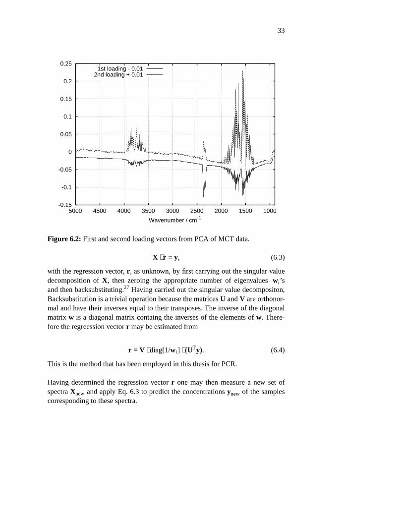
As a simple example of this graphical interpretation, PCA on a data matrix con-sisting of 40 single beam spectra taken with 10 minutes intervals, measured withan empty beam using an MCT detector were carried out. The first measurementwas carrried out 10 minutes after filling the detector with liquid N2. Figure 6.1shows the first diagonal values w. The figure reveals two dominating orthogonalvariations in the data set. Figure 6.2 shows the first and second loading vectorsV1 and V2. The first loading vector is seen to model the sensitivity of the detec-tor which is the broad shape of the baseline Moreover, the contents of H2O andCO2 in the empty beam are represented by OH bending vibrations at2000 − 1400 cm−1, OH stretching vibrations at 4000 − 3500 cm−1 and assymetri-cal stretch vibrations of CO at 2300 cm−1. There is a covariance between the sen-sitivity of the detector and the contents of water and carbon dioxide in the mea-sured data set. The two variations are physically independent. There is no causalconnection, yet they both vary monotonically with time. Detector sensitivityincreases monotonically and H2O, and CO2 concentration decrease monotoni-cally. Both variations converge tow ards som stable value. This means that thetwo types of variations may not be completely separated. Figure 6.3 shows ascore plot of the first and second scores, U1 and U2. Each data point represents aspectrum, such that the essential variation of the spectra are represented by twovariables. One observes that the detector stabilizes within 1 hour as the single-beam intensity modeled by the first score converges. A much slower convergenceis the gradual removal of H2O and CO2 by the continuous purge of the

32

0

2e-08

4e-08

6e-08

8e-08

1e-07

1 2 3 4

diagonal value

Figure 6.1: Diagonal values from PCA of MCT data.

instrument which is modeled by the second principal component. The third load-ing vector, which is not shown, contains information related to CO2 alone. Therest of the loading vectors contains noise and may be disregarded.

6.2. Principal component regression

The orthogonality and reduced dimension of the new coordinate system makesthe scores ideally suited for multiple linear regression (MLR) when one wishes touse the spectra for calibration with some control value y, typically a concentra-tion, attached to each measured spectrum. Carrying out multiple linear regres-sion on the transformed data set emerging from the principal component analysisis known as principle component regression (PCR).

The result of the PCR calibration is a regression vector, r, which depends on thenumber of principal components that has been retained in the data set. Thisregression vector, r, is then multiplied as a dot product with a spectrum to predicta concentration value belonging to the spectrum.

This is equivalent to finding the best solution, in a least squares sense, to theequation

33

-0.15

-0.1

-0.05

0

0.05

0.1

0.15

0.2

0.25

100015002000250030003500400045005000

Wavenumber / cm-1

1st loading - 0.012nd loading + 0.01

Figure 6.2: First and second loading vectors from PCA of MCT data.

X ⋅ r = y, (6.3)

with the regression vector, r, as unknown, by first carrying out the singular valuedecomposition of X, then zeroing the appropriate number of eigenvalues wi’sand then backsubstituting.27 Having carried out the singular value decompositon,Backsubstitution is a trivial operation because the matrices U and V are orthonor-mal and have their inverses equal to their transposes. The inverse of the diagonalmatrix w is a diagonal matrix containg the inverses of the elements of w. There-fore the regreession vector r may be estimated from

r = V ⋅ diag[1/wi] ⋅ (UTy). (6.4)

This is the method that has been employed in this thesis for PCR.

Having determined the regression vector r one may then measure a new set ofspectra Xnew and apply Eq. 6.3 to predict the concentrations ynew of the samplescorresponding to these spectra.

34

-3.5e-05

-3e-05

-2.5e-05

-2e-05

-1.5e-05

-1e-05

-5e-06

0

5e-06

1e-05

1.5e-05

-5e-05 0 5e-05 0.0001 0.00015 0.0002 0.00025

2 P

C

1 PC

1

2

3

4

5

6

7

8

9

10111213141516171819202122232425262728293031323334353637383940

Figure 6.3: Score plot of MCT data first vs. second score.

6.3. Partial least squares regression

Another calibration technique, known as partial least squares regression54

(PLSR), is also commonly used. This technique takes advantage of the y valueswhen transforming the data set, such that spectral variations in X that correlateswith the variation y are selected. In this fashion, signals buried below more domi-nating irrelevant variations are extracted. This frequently yields simpler modelswith fewer principal components, now called PLS factors. The price one has topay for this advantage is that the axes in the transformed coordinate system areno longer orthogonal and that the model is more sensitive to over-fitting.54, 55 Aswith PCR, PLSR results in a regression vector r which is multiplied with a spec-trum as a dot product to obtain an estimate of the concentration value correspond-ing to the measured spectrum. As a general idea, it is a useful check of the cali-bration process to use both these methods to construct the regression vector andcompare the obtained results. Typically, differences between regression vectorsobtained by the two methods is a sign that something unhealthy is going on.Keeping too many components leads to models where spurious correlations causepoor prediction of concentrations belonging to spectra not included in the calibra-tion model. Principal component regression has generally been favored by theauthor because of the neutral behavior with regard to concentration values and

35

lack of tendency to over-fit compared to PLSR. For most of the experimentsupon which this thesis is based, sample variability is small and the differencebetween the two methods of calibration is small. The advantages of PLSR doesnot then emerge, when compared with PCR on the data from these experiments.Even so, both methods of calibration have been applied and results compared,choosing the optimal calibration model as the best of both methods.

6.4. Effect of over-fitting on the regression vector

It is instructive to look at the way the regression vector changes as more andmore principal components are included in the model. Typically, the regressionvector begins with a broad shape which does not resemble the spectral shape ofthe control variable it should predict. As more principal components are added,the regression vector resembles the spectral shape of the pure control variable. Ifinterferences are present, the regression vector is then given a lower weight inthose spectral regions where the interferences reduce the correlation between thecontrol variable and the data or it is adjusted to compensate for the change causedby the interference. When over-fitting takes place, the regression vector tends toweigh the strongest peak of the control variable and to oscillate in such a way asto average out the spectral values found elsewhere in the spectrum. The multi-variate nature of the calibration is reduced and one is left with essentially an uni-variate model which is much more sensitive to changes in the spectrum that hasnot been included in the calibration. This is exemplified by the regression vectorsfor predicting urea concentrations from single-beam spectra presented in Paper I,Fig. 10. By retaining more components, the PLSR calibration will give increas-ingly accurate prediction of the data upon which it is built. Application of themodel to predict concentrations of an independent data set will then result in alarge error, often manifested as a bias. This error is caused by a change in spec-tral structure in the new data set combined with the rapid oscillation and univari-ate nature of the over-fitted regression vector.

6.5. Influence of signal-to noise ratio on the predictive ability of calibrationmodels.

Given a very accurate regression vector, r, from a calibration model based on alarge number of samples and a single spectrum from a sample we wish to esti-mate the concentration of that sample. One may then show, with a simple argu-ment given in paper II, that the uncertainty in the determination of the concentra-tion is proportional to the square root of the number of independent spectralpoints containing information that correlates with the concentration and inverselyproportional to the noise level of these spectral points. The noise level is there-fore a stronger factor than the number of independent spectral points, when onewishes to optimize the predictive ability of a model. The number of independent

36

spectral points is important in the sense that it determines how many independentvariations the model can handle and therefore compensate for spectral interfer-ences.

6.6. Validation of calibration models

Clearly, the construction of a calibration model has as its object to predict theconcentration of new samples from their spectra. The ability to do so should beverified by testing the calibration model on an independently measured data set.

Testing is frequently done by splitting a measured data set in two nearly equalsubsets, constructing the model from one of the two subsets, and predicting theconcentrations of the other. If the data set is split in two at random, such thatthey are intertwined in time, the model will in principle only interpolate whentested on the other part of the data set. This is also the case for cross-validationschemes where the model is constructed repeatedly from parts of the data andtested on the remaining parts. These are the predominant validation methodsfound in the current literature.

Successful testing of a calibration model is more impressive when the test set ismeasured at a separate later time, possibly by another person, and even better ona different instrument. In the latter case one speaks of transfer of calibration. Iftransfer of calibration is possible, the calibration becomes commercially interest-ing, provided there is a demand for measurements of the control variable,because calibration is an expensive procedure to carry out. This topic currentlyreceives considerable attention.56 One method is based on calibration on a refer-ence instrument. To make a transfer of calibration possible, the spectrum of astandard sample is measured on this reference instrument. By measuring thespectrum of the standard sample on other instruments and adjusting this spectrumin software to match the one measured on the reference instrument, sufficientsimilarity of the spectra are obtained to make the transfer of calibration possible.

The calibrations presented in this thesis have consistently been validated fromcompletely independent test sets measured at least one day later than the calibra-tion set.

6.7. Validation measures

The common method of quantifying the quality of the predicted concentrationsfrom a data set is by calculation of the root-mean-square error of prediction,RMSEP, giv en as

37

RMSEP =

1

n

n

i=1Σ(yi − yi)

2

12

(6.5)

where n is the number of samples y are the predicted concentrations and y arethe corresponding reference values. The same formula may be used to estimatethe calibration models internal consistency by applying it to the data upon whichit is built. In that case one speaks of the root-mean-square error of calibration,RMSEC. One may further distinguish between systematic errors, most com-monly manifested as a bias, and statistical errors. The presence of a bias indicatesproblems with drift or diffent types of samples in calibration and test set,whereas statistical errors result from noise.

6.8. Chemometry and instrument configuration.

Noise in a given spectral region destroys the possible correlation with a variationin the y vector. Therefore PCR and PLSR will create regression vectors that givea high weight to spectral regions with low noise if it contains a correlation withthe y vector. Paper II demonstrates that the noise level changes strongly withwavenumber for a given choice of pathlength when measurements of aqueoussolutions are carried out. Therefore, one may predict in advance, solely from theabsorption spectrum of the samples, the spectral regions that will be selected bythe regression vector. This was a major motivation for paper II. It is commonlyassumed in chemometric analysis, that the noise level in spectral data are roughlyidentical across a spectrum. Consequently, the results of the analysis are inter-preted as intrinsic properties of the samples and not as properties of the instru-mental configuration. For chemometric analysis of aqueous solutions, this com-mon assumption does not hold. The noise level depends very strongly on thechoice of transmission pathlength, such that the results of the chemometric analy-sis will be different if this pathlength is changed. In this case it will be necessaryto compare the results of the chemometric analysis with the noise levels in thespectra to obtain the correct information of the intrinsic properties of the sample.As pointed out in paper II, the chosen pathlength selects a narrow spectral regionwhere the SNR is optimized. One may therefore profitably optimize this spectralregion by filtering out light in the other spectral regions and maximize the inten-sity in the chosen region. If information in different spectral regions are required,and it is possible to carry out more than one measurement, then one should do sowith different choices of pathlength. Interestingly, Hirschfeld has suggested theuse of a stepped transmission cell to improve the dynamic range of transmissionmeasurements as early as 1978.57 The author has seen no other publicationswhere this technique has been applied.

38

7. The near and mid infrared absorption spectrum of water

Passing from a description of the measurement and data analysis techniquesemployed in this work, we will now dev ote our attention to the properties of themeasured samples and their influence on possible applications. This thesis isconcerned with measurements of trace components in aqueous solutions. Thenear and mid infrared spectra of such solutions are dominated by the absorptionspectrum of water which is described in this chapter. Much information concern-ing the fysics and structure of water and aqueous solution is contained in the fivevolume treatise on water by Franks1, 58-61

Water, H2O, in the liquid state has an absorption spectrum as shown in Fig. 7.1.The data has been taken from paper III and has been measured at 37 °C. Themost recent compilation of the absorption spectrum of water at 25 °C is given byBertie and Lan.62 The strongest absorption bands are the OH stretch band ν1,3

found betweeen 3800 and 3000 cm−1 and the OH bend band, ν2, at 1644 cm−1.At 800 to 500 cm−1 one finds a broad strong absorption band caused by collectivemotion of water molecules, the so-called libration band νL. These three bandsare not resolved in Fig. 7.1. A combination band ν2 + νL is found at 2100 cm−1

and a combination band ν1,3 + ν2 is found at 5160 cm−1. Overtone bands arefound at approximately 6900 cm−1. The major absorption bands are listed inTable 7.1.

Wa venumber / cm−1 Vibration mode

500-800 Libration, broad1644 H-O-H bend2128 H-O-H bend + libration3250 Fermi enhanced overtone of H-O-H bend3450 O-H symmetric stretch3600 O-H asymmetric stretch5160 H-O-H bend + (a)symmetric O-H stretch7050 O-H stretch overtone and combination

Table 7.1: Absorption bands of water as listed by Venyaminov andPrendergast.63

Signals from trace components are superposed on this absorption spectrum, andan absorption spectrum of an aqueous solution containing any trace component ina clinically relevant concentration will be indistinguishable by eye from theabsorption spectrum of water shown in Fig. 7.1. Information about the structureof liquid water may be extracted from the water absorption spectrum and fromit’s dependency on temperature. For this purpose, interest focuses on the main

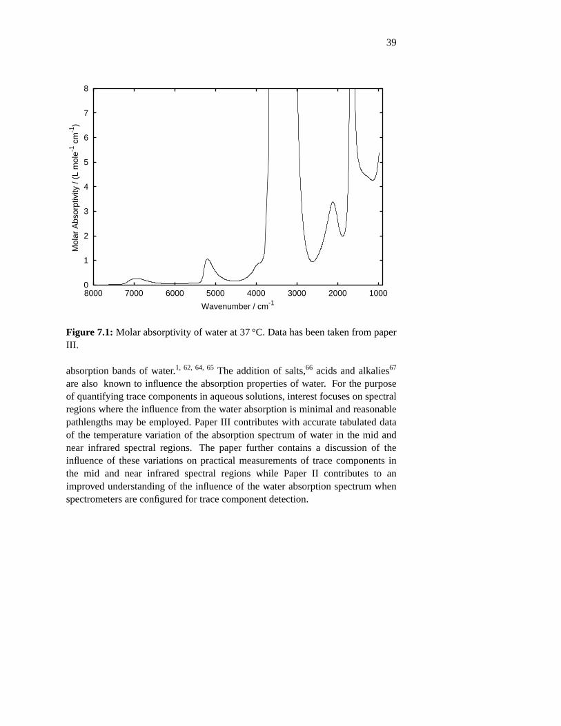
39

0

1

2

3

4

5

6

7

8

10002000300040005000600070008000

Mol

ar A

bsor

ptiv

ity /

(L m

ole-1

cm

-1)

Wavenumber / cm-1

Figure 7.1: Molar absorptivity of water at 37 °C. Data has been taken from paperIII.

absorption bands of water.1, 62, 64, 65 The addition of salts,66 acids and alkalies67

are also known to influence the absorption properties of water. For the purposeof quantifying trace components in aqueous solutions, interest focuses on spectralregions where the influence from the water absorption is minimal and reasonablepathlengths may be employed. Paper III contributes with accurate tabulated dataof the temperature variation of the absorption spectrum of water in the mid andnear infrared spectral regions. The paper further contains a discussion of theinfluence of these variations on practical measurements of trace components inthe mid and near infrared spectral regions while Paper II contributes to animproved understanding of the influence of the water absorption spectrum whenspectrometers are configured for trace component detection.

40

8. Trace component quantification in aqueous solutions

This chapter provides a brief description of the published results, regarding thequantification of trace components in aqueous solutions, that have influenced thework presented in this thesis. These works have been focused on clinical applica-tions. This could be regarded as a much to narrow focus, but most of the clinicalapplications require measurements of very low concentrations of molecules invery complex liquids. Moreover, the methods claimed to be successful arerequired to pass strict tests if anyone are to invest in their development into acommercial product as the consequences of instrument failure may have sev ereconsequences. The most studied biological aqueous solutions of clinical interestare blood, blood serum. urine, and recently, spent dialysate. In addition amnioticfluid, and oral mucosa have been studied.8, 68 A comprehensive review of the nearand mid infrared applications of near and mid infrared spectroscopy with a largesection devoted to measurements on biological fluids is given by Heise.69 Vonachand Kellner have analyzed whole blood for glucose in the mid infrared regionemploying a transmission cell. They achieved standard errors of prediction of13. 1 mg/dl.13 Heise and co-workers have slightly lower standard errors of predi-cion for glucose, 9. 8 mg/dl using an ATR micro-Circle cell.70 Similar results areobtained with the same technique by Haaland and co-workers.9 Heise and co-workers have also measured protein, cholesterol and urea in whole blood.69 Theconcentrations of urea, creatinine, sulphate, and phosphate has been determinedin urine by the same authors.70 standard error of prediction for urea was 13 mM.A slightly higher standard error of prediction has been obtained by Shaw,Kotowich, and Mantsch by near-infrared transmission spectroscopy, who alsodetermined creatinine and protein.71

Arnold, Small and co-workers have concentrated their efforts in the combinationband region, 4000 − 5000 cm−1. They hav e demonstrated this spectral region tobe well suited for the determination of glucose, urea and other components indifferent fluids including blood serum and dialysate.72, 73 In studying the bloodserum, the standard error of prediction for glucose was 23 mg/dl. These authorhave carried out extensive inv estigations based on model systems with syntheti-cally prepared samples to develop calibrations that are insensitive to temperaturevariations,12 or are based on single-beam spectra.52 The same authors have inv es-tigated the possible use of the 6500 − 5500 cm−1 spectral region, containing over-tone bands, for the determination of glucose, urea and other components.73, 74

The primary motivation for investigating the overtone band region is found in theweak absorption of water that allows deeper penetration of light. This is impor-tant in non-invasive measurements for biological purposes. The main example isthe, yet to come, non-invasive glucose sensor for diabetic patients. Unfortunately,the broad and weak nature of the overtone bands found in this spectral region

41

makes it much less suited than the combination band region.

Commercial systems exist for measurement of trace components in milk andwine using mid infrared transmission spectroscopy.75 The high concentrations ofglucose, fructose and lactose in sugar cane juice and fruit juices may be deter-mined with both mid and near infrared transmission spectroscopy.76, 77

Three of the papers contained in this thesis contributes to this field. Paper Idemonstrates measurements of urea and glucose in aqueous solutions in thiscombination band 5000 − 4000 cm−1 spectral region with a dual-beam instru-ment. Paper IV presents measurements with a similar dual-beam instrument inthe same spectral region for the determination of urea in spent dialysate. Paper Vpresents measurements of urea, glucose and phosphate in spent dialysate by midinfrared transmission spectroscopy in the 100 − 1500 cm−1 spectral region.

42

9. Haemodialysis treatment

This chapter gives a brief description of the causes, the consequenses and thetreatment of chronical renal failure. The correct treatment is currently difficult todetermine and the monitoring of trace components by FT-IR spectroscopy is apossible diagnostic tool for that purpose. The present description has been basedmainly on the book edited by Eidemark and Bro.78

There are about 4000 patients with chronical insufficent renal function in Den-mark, which has a population of approximately 6 million. Of these, approxi-mately 1600 are subject to haemodialysis treatment. A simple scaling of thesefigures to a global population of 6 × 109 yields that approximately 4 million peo-ple suffers from chronical renal failure. This estimate is probably to high. Renalfailure is mainly a result of a number of diseases that are more prevalent in olderpatients. It may be more accurate to state, that 0.07% of the population of thewestern world suffers from chronical renal failure. In Denmark, 20% of thepatients with renal failure have diabetes. Vascular diseases are responsible for11% of the cases. Another 26% of the cases are caused by Pyelonephritis andGlomerulonephritis, which are inflammatory disesases. Renal failure results inan accumulation of end stage products of the metabolic processes taking place inthe body. Metabolic acidosis, overhydration hyperphospataemiea, hyperkalaemiaand hypertension arise. Arterial hypertension is also a common cause of renalfailure. The symptoms of renal failure are few. The most common symptom isfatigue. In more severe cases, anaemia, loss of appetite, dry skin, and paresthesiaoccur. Nearly all organs are influenced by an uremic condition, including theimmune defence system, such that a patient with renal failure has less resistanceagainst infections. With no treatment, complete renal failure is lethal.

Patients with renal failure are subject to haemodialysis treatment. In this treat-ment, the removal of toxins from the blood are carried out by an artificial kidney.Blood from the patient is pumped out of the patient, through a filter, where aporous membrane separates it from a stream of dialysate, and again into thepatient. The difference in osmotic pressure across the porous membrane results ina diffusion of toxic components from the blood to the dialysate. A pressure gra-dient across the membrane is used to remove exess liquid from the patient tomaintain his dry weight. In this way, the function of the kidneys are mimickedby the dialysis station. The pore size of the porous membrane determines thesize of the molecules that may be removed. Numerous small and medium sizemolecules are removed by this process. Which of these that are toxic is undermuch debate. The rate of removal depends on the size of the molecule, the filterpore size, and a number of physiological factors. Some molecules are mainlyextracellular and some are intracellular. Their removal is then also determined bytheir transport properties from and to the cells.

43

The efficiency of the dialysis depends on a number of parameters, such as filtertype, blood flow, pressure gradient, and quality of the vascular access. A numberof these parameters is individually determined for each patient. The treatmentduration is long and has to be undertaken regularly. Patients are typically treatedthree to four hours three days a week. The correct dialysis dose is critical for thepatient and monitoring the dialysis dose is therefore important. Underdialyzing apatient has severe health consequences. The current estimate of dialysis dose isbased on the removal of urea. It is uncertain whether urea is toxic in itself, but ithas been shown, that serum urea concentration correlates with symptoms andsigns of renal failure. Urea also provides information about the patients nitrogenbalance. It is the end-product of the protein breakdown process, and is directlyrelated to the protein catabolic rate.79 The dialysis dose is estimated from thedimensionless expression Kt/V where K is the dialyzer urea clearance, t is thetreatment time and V is the urea distribution volume of the patient. This figure isrequired to be above 1.2 when three weekly treatments are carried out. The Kt/Vvalue is usually estimated by the Daugirdas formula

Kt/V = − ln(R − 0. 008t) + (4 − 3. 5R)U /W , (9.1)

where t is the treament time in hours, R is the ratio of urea concentration in bloodsamples taken pre- and post- treatment, U is the ultrafiltration in L, and W is thepatients weight in kg after treatment. A rough estimate is given by the formula

Kt/V = 0. 093Kt/W , (9.2)

where K is the in-vitro clearance of the filter, at a giv en blood flow, in ml/min.These estimates are neccesarily based on assumptions of a haemodialysis treat-ment that are following a well defined pattern. Even in patients that are in stablecondition, these estimates may vary with 10-20%. Moreover, the estimate fromthe Daugirdas formula is made post-treatment and adjustment of treatment is usu-ally not carried out on the basis of a single estimate of Kt/V . Since blood samplesare taken monthly, this means that it may be two months before a needed adjust-ment is carried out. Another estimate of dialysate dose is the urea reduction ratio(URR),

URR = (1 − R), (9.3)

where R is the ratio of urea concentrations in blood samples taken pre- and post-treatment as above. This ratio should be above 65% with three weekly treatments.

The continuous measurement of urea removal during haemodialysis treatmentwill be a useful diagnostic tool which may be used to control and optimize thetreatment. In paper V, dual-beam FT-IR spectroscopy is used to carry out such anon-line monitoring. Other efforts to monitor urea concentrations in spentdialysate by optical methods include the works by Arnold, Eddy, Flannigan and

44

Olesberger,73, 80 who also work with FT-IR spectroscopy in the spectral region5000 − 4000 cm−1. A Ph.D dissertation81 presents a method based on differentialmeasurements at wav elengths 1485, and 1393 nm. Non-optical methods for theon-line monitoring of urea concentrations in spent dialysate exists. They arebased on urease chemistry, or conductivity measurements caused by changes inionic concentration in the dialysate. They are therefore either requiring reagents,or monitoring a secondary effect assumed to correlate with the urea concentra-tion. An optical method would possess strong advantages over these methods inspeed and accuracy. As mentioned, urea is only a secondary indicator of toxicityas it is not itself toxic. High concentrations of phosphate are known to be toxic,however. Hyperphosphateamia is linked to hyperparathyroidism, calcification,hypertension, and left ventricular hypertrophy.82 A call for continuous monitoringof phosphate removal has recently been made.82 Paper IV demonstrates, thatphosphate may be measured with mid infrared spectroscopy together with ureaand glucose. It is therefore possible to monitor these three components on-linewith mid infrared transmission spectroscopy.

45

Acknowledgements

The supervision received from Senior Research Scientists Jimmy Bak and PeterE. Andersen of Risø National Laboratory, and Professor Stefan Andersson-Engels of Lund Institute of Technology is gratefully acknowledged.

The help and encouragement from the colleagues at the Optics and Fluid Dynam-ics Department, Risø National Laboratory, is gratefully acknowledged. Thealways friendly and helpsome colleagues at Lund Institute of Technologydeserves special thanks for assistance with many adminstrative details and for thenice atmosphere that has prevailed during my particiption in courses. SeniorResearch Scientist Sønnik Clausen of Risø National Laboratory deserves specialthanks for having the foresight to purchase an FT-IR spectrometer with two inputports when one would suffice for his purposes. Dr. Lars Thrane and Dr. AndreasTycho are to blame for repeated intrusions and continuous demands for coffee.As head of scientific programme, Dr. Steen Hanson is to blame for luring me intothis project. I beg his forgiveness for my untimely use of binoculars.

Financial support from the Danish Research Academy is gratefully acknowl-edged.

46

Summary of papers

Paper I presents measurements with a dual-beam, optical null, FT-IR instrument,also capable of measuring traditional single-beam spectra, for the quantificationof urea and glucose in the near infrared spectral region 5000 − 4000 cm−1. Theresults are compared with traditional single-beam measurements. The compari-son shows that the dual-beam technique eliminates instrument variations and iscapable of providing data that may be modeled with fewer factors yielding lowererrors of prediction and better stability.

Paper II presents an analysis of noise levels in measurements of spectra of purewater and aqueous solutions at different transmission cell pathlengths. An analyt-ical model that predicts the optimal pathlength for near infrared transmissionmeasurements of aqueous solutions explains the results. The paper emphasizesthat transmission cell pathlength should be chosen from the absorption propertiesof the solvent, and that it is favorable to increase pathlength when the detectorwould otherwise saturate. Apparent discrepancies found in the literature areexplained by these results.

Paper III presents accurate measurements of the temperature variation of theabsorption spectrum of water in the mid and near infrared regions. The mea-sured molar absorptivities of water are compared to existing values found in theliterature and tabulated. The temperatures are restricted to the physiologicallyrelevant range from 30 to 42 °C. The fundamental stretching and bending bandsof water are excluded. The effect of temperature on aqueous glucose solutions inthe two spectral regions is also measured. The practical consequences of temper-ature variations and matrix effects in the two spectral regions, when trace compo-nents must be quantified, are discussed.

Paper IV presents on-line measurements of urea concentration in dialysate dur-ing treatment with the dual-beam, optical null, instrumentation presented in paperI. A simple calibration model based on synthetically prepared dialysate samplesis used to predict the urea concentrations. The dual-beam instrument is demon-strated to provide accurate mesurements over a period of one month.

Paper V presents measurements of spent dialysate in the mid infrared spectralregion for the simultaneous quantification of urea, glucose, and phosphate. Theaccuracy of the predicted concentrations are found to be comparable with that ofthe reference method for each of the three components.

Contributions to the papers by the author:

All work were carried out by the author with the following exceptions: Glucosemeasurements in paper I were carried out by first year students from RoskildeUniversity as acknowledged in that paper. In paper IV and V, clinical chemicalanalysis of dialysate samples were carried out by the Clinical Chemistry

47

Department at the Copenhagen University Hospital. In paper V part of the mea-surements were carried out by T. Begovic of Risø National Laboratory. S. D.Ladefoged of the Nephrological Department, Copenhagen University Hospitalbore the responsibility for the care and treatment of the patients involved inpapers IV and V and contributed to the discussions of the clinical implications ofanalysis of dialysate. The manuscripts were written by the author with assistancefrom the co-authors. The author has been corresponding author of all the papers;any fault contained therein is on his head.

48

REFERENCES

1. Felix Franks (ed.), The Physics and Physical Chemistry of Water, Water acomprehensive treatise, 1, Plenum Press, New York (1972).

2. Linus Pauling, General Chemistry, Dover Publications Inc., New York(1970).

3. Handbook of Near-Infrared Analysis, Marcel Dekker, Inc., New York(2001).

4. Infrared and Raman Spectroscopy of Biological Materials, Marcel Dekker,Inc., New York (2000).

5. H. Zeller, P. Novak, and P. Landgraf, “Blood glucose measurement byinfrared spectroscopy,” Int. J. Artif. Organs, 12, 2, pp. 129-135 (February1989).

6. Prashant Bhandare, Yitzhak Mendelson, Robert A. Peura, GuntherJanantsch, Jurgen D. Kruse-Jarres, Ralf Marbach, and Michael H. Heise,“Multivariate Determination of Glucose in Whole Blood Using PartialLeast-Squares and Artificial Neural Networks Based on Mid-InfraredSpectroscopy,” Appl. Spectrosc., 47, 8, pp. 1214-1221 (1993).

7. H. M. Heise and A. Bittner, “Investigation of Experimental Errors in theQuantitative Analysis of Glucose in Human Blood Plasma by ATR-IRSpectroscopy,” J. Mol. Struct., 348, pp. 21-24 (1995).

8. H. M. Heise and R. Marbach, “Human Oral Mucosa Studies with VaryingBlood Glucose Concentration by Non-Invasive ATR-FT-IR Spectroscopy,”Cellular and Molecular. Biol., 44, 6, pp. 899-912 (1999).

9. Kenneth J. Ward, David M. Haaland, M. Ries Robinson, and R. PhilipEaton, “Post-Prandial Blood Glucose Determination by Quantitative Mid-Infrared Spectroscopy,” Appl. Spectrosc., 46, 6, pp. 959-965 (1992).

10. Jason J. Burmeister and Mark A. Arnold, “Evaluation of MeasurementSites for Noninvasive Blood Glucose Sensing with Near-Infrared Transmis-sion Spectroscopy,” Clin. Chem., 45, 9, pp. 1621-1627 (1999).

11. Hoeil Chung, Mark A. Arnold, Martin Rhiel, and David W. Murhammer,“Simultaneous Measurements of Glucose, Glutamina, Ammonia, Lactate,and Glutamate in Aqueous Solutions by Near-Infrared Spectroscopy,”Appl. Spectrosc., 50, 2, pp. 270-276 (1996).

12. Kevin H. Hazen, Mark A. Arnold, and Gary W. Small, “Temperature-Insensitive Near-Infrared Spectroscopic Measurement of Glucose in Aque-ous Solutions,” Appl. Spectrosc., 48, 4, pp. 477-483 (1994).

13. R. Vonach, J. Buschmann, R. Falkowski, R. Schindler, B. Lendl, and R.Kellner, “Application of Mid-Infrared Transmission Spectrometry to the

49

Direct Determination of Glucose in Whole Blood,” Appl. Spectrosc., 52, 6,pp. 820-822 (1999).

14. Takuo Yano, Takatoshi Funatsu, Ken-ichiro Suehara, and Yasuhisa Nakano,“Measurement of the concentrations of glucose and citric acid in the aque-ous solution of a blood anticoagulant using near infrared spectroscopy,” J.Near Infrared Spectrosc., 9, pp. 43-48 (2001).

15. Gilwon Yoon, Yoen-Joo Kim, and Sangjoon Hahn, “Determination of glu-cose in whole blood samples by mid-infrared spectroscopy,” Appl. Opt., 42,4 (1 February 2003).

16. Shmuel Argov, Jagannathan Salman, Ramesh, Ahmad Salman, Igor Sinel-nikov, Jed Goldstein, Hugo Guterman, and Shaul Mordechai, “Diagnosticpotential of Fourier-transform infrared microspectroscopy and advancedcomputational methods in colon cancer patients,” J. Biomed. Opt., 7, 2, pp.248-254 (April 2002).

17. Yun Xiang Ci, Ti Yu Gao, Jun Feng, and Zhen Quan Guo, “Fourier Trans-form Infrared Spectroscopic Characterization of Human Breast Tissue:Implications for Breast Cancer Diagnosis,” Appl. Spectrosc., 53, 3, pp.312-315 (1999).

18. Alex Pevsner and Max Diem, “Infrared Spectroscopic Studies of MajorCellular Components. Part I: The Effect of Hydration on the Spectra ofProteins,” Appl. Spectrosc., 55, 6, pp. 788-793 (2001).

19. A.M.K. Nilsson, D. Heinrich, J. Olajos, and S. Andersson-Engels, “Nearinfrared diffuse reflection and laser-induced fluorescence spectroscopy formyocardial tissue characterisation,” Spectrochim. Acta Part A, 53, pp.1901-1912 (1997).

20. N. B. Colthup, L. H. Daly, and S. E. Wiberley, Introduction to Infrared andRaman Spectroscopy, Academic Press, San Diego, California (1990).

21. Donald L. Pavia, Gary M. Lampman, and George S. Kriz, Introduction toSpectroscopy, Saunders College Publishing, Orlando,Florida (1996).

22. David R. Lide, (ed.), Handbook of Chemistry and Physics, pp. 9-74, CRCPress, Boca Raton, Florida (1995).

23. Peter R. Griffiths and James A. de Haseth, Fourier Transform InfraredSpectrometry, John Wiley & Sons, New York (1986).

24. Tomas Hirschfeld, “Quantitative FT-IR A detailed look at the problemsinvolved” in Fourier Transform Infrared Spectroscopy Applications toChemical Systems, ed. John R. Ferraro and Louis J. Basile, 2, AcademicPress, Orlando, Florida (1979).

50

25. J. E. Bertie, “Apodization and Phase Correction” in Analytical Applicationsof FT-IR to Molecular and Biological Systems, ed. J. R. Durig, NAT OAdvanced Study Institutes, Series C -- Mathematical and Physical Sci-ences, 57, D. Reidel Publishing Company, Dordrecht: Holland (1980).

26. E. Oran Brigham, The Fast Fourier Transform and its Applications, Pren-tice Hall, Englewood Cliffs,New Jersey (1988).

27. William H. Press, Saul A. Teukolsky, William T. Vetterling, and Brian P.Flannery, Numerical Recipes in C The Art of Scientific Computing, Cam-bridge University Press, Cambridge (1995).

28. M. Shane Hutson and Mark S. Braiman, “Direct Phase Correction of Dif-ferential FT-IR Spectra,” Appl. Spectrosc., 52, 7, pp. 974-984 (1998).

29. H. Sakai, G. A. Vanasse, and M. L. Forman, “Spectral Recovery in FourierSpectroscopy,” J. Opt. Soc. America, 58, 1, pp. 84-90 (1968).

30. D. B. Chase, “Phase Correction in FT-IR,” Appl. Spectrosc., 36, 3, pp.240-244 (1982).

31. Michael A. Kinch, “Fundamental Physics of Infrared Detector Materials,”J. Electron. Mat., 29, 6, pp. 809-817 (2000).

32. N. J. Harrick,, Internal reflection spectroscopy, Interscience Publishers,,New York (US), (1967).

33. Jan D. Miller, Mehmet Hancer, and Roger P. Sperline, “Anomalous Disper-sion Effects in the IR-ATR Spectroscopy of Water,” Appl. Spectrosc., 54, 1,pp. 138-143 (2000).

34. P. Fellget, “Les Progres Recents en spectroscopie interferentielle,” Belle-vue, Colloq. Int. C.N.R.S., p. 53 (1957).

35. Hillel Bar-Lev, “A Dual-Beam Infrared Interferometer Spectrometer,”Infrared Phys., 7, pp. 93-98 (1967).

36. M. J. D. Low and H. Mark, “SO2 Detection by Dual-Beam Fourier Trans-form Spectroscopy,” Water, Air, and Soil Pollution, 1, pp. 3-6 (1971).

37. George A. Vanasse, Randall E. Murphy, and Floyd H. Cook, “Double-beaming technique in Fourier spectroscopy,” Appl. Opt., 15, 2, pp. 290-291(February 1976).

38. Orr Sheperd, William Reidy, and George A. Vanasse, “Background sup-pression and spectral detection using double-beam interferometry: instru-mentation,” Proc. SPIE, 191, pp. 64-70 (1979).

39. Theodore Zehnpfennig, Saul Rappaport, and George A. Vanasse, “Back-ground suppression and spectral detection using double-beam interferome-try: measurements,” Proc. SPIE, 191, pp. 71-78 (1979).

51

40. Peter R. Griffiths, “Recent Applications of Fourier Transform InfraredSpectrometry in Chemical and Environmental Analysis,” Appl. Spectrosc.,31, 6, pp. 497-505 (1977).

41. H. R. Chandrasekhar, L. Genzel, and J. Kuhl, “Double-beam Fourier Spec-troscopy with interferometric background compensation,” Opt. Commun.,17, 1, pp. 106-110 (April 1976).

42. L. Genzel, H. R. Chandrasekhar, and J. Kuhl, “Double-beam Fourier spec-troscopy with two inputs and two outputs,” Opt. Commun., 18, 3, pp.381-386 (August 1976).

43. L. Genzel and J. Kuhl, “A New Version of a Michelson Interferometer forFourier Transform Infrared Spectroscopy,” Infrared Phys., 18, pp. 113-120(1978).

44. Donald Kuehl and Peter R. Griffiths, “Dual-Beam Fourier TransformInfrared Spectrometer,” Anal. Chem., 50, 3, pp. 418-422 (March 1978).

45. Maria M. Gomez-Taylor and Peter R. Griffiths, “On-Line Identification ofGas Chromatographic Effluents by Dual-Beam Fourier Transform InfraredSpectroscopy,” Anal. Chem., 59, 3, pp. 422-425 (March 1978).

46. G. J. Kemeny and P. R. Griffiths, “Improved Sensitivity in Dual-BeamFourier Transform Infrared Spectroscopy,” Appl. Spectrosc., 34, 1, pp.95-97 (1980).

47. C. P. Tripp and M. L. Hair, “Transmission Infrared Spectra of AdsorbedPolymers Using a Dual-Beam FT-IR Instrument,” Appl. Spectrosc., 46, 1,pp. 100-106 (1992).

48. C. P. Tripp and M. L. Hair, “Quantitative Infrared Spectroscopy ofPolystyrene Block Copolymer Adsorbed on Mica,” Langmuir, 8, pp.241-244 (1992).

49. Donald L. Beduhn and Robert L. White, “Advantages of Dual-Beam Inter-ferometry in Fourier Transform Infrared Spectrometry,” Appl. Spectrosc.,40, 5, pp. 628-632 (1986).

50. Philip R. Bevington and D. Keith Robinson, Data Reduction and ErrorAnalysis for the Physical Sciences, McGraw-Hill Book Company, NewYork (1992).

51. Peter R. Griffiths and Bryan T. Bowie, “Measurement of the Sensitivityand Photometric Accuracy of FT-IR Spectrometers,” Appl. Spectrosc., 54,8, pp. 1192-1202 (2000).

52. Mark A. Arnold, Geng Lu, Xiangji Zhou, and Gary W. Small, “Multivari-ate Calibration Models Based on the Direct Analysis of Near-Infrared Sin-gle-Beam Spectra,” Appl. Spectrosc., 51, 9, pp. 1330-1339 (1997).

52

53. Svante Wold, Kim Esbensen, and Paul Geladi, “Principal ComponentAnalysis,” Chemo. Intel. Lab. Sys., 2, pp. 37-52 (1987).

54. Harald Martens and Tormod Næs, Multivariate calibration, John Wiley &Sons, New York (1989).

55. Neil A. Butler and Michael C. Denham, “The peculiar shrinkage propertiesof partial least squares regression,” J. Royal Stat. Soc. B, 62, 3, pp. 585-593(2000).

56. Eric Bouveresse and Bruce Campbell, “Transfer of Multivariate Calibra-tion Models Based on Near-Infrared Spectrscopy” in Handbook of Near-Infrared Analysis, ed. Donald A. Burns and Emil W. Ciurczak, pp.241-260, Marcel Dekker, Inc., New York (2001).

57. T. Hirschfeld, “Dynamic Range Improvement in Fourier TransformInfrared Spectrometry,” Anal. Chem., 50, 8, p. 1225,1226 (July 1978).

58. Felix Franks (ed.), Water in Crystalline Hydrates Aqueous Solutions ofSimple Nonelectrolytes, Water a comprehensive treatise, 2, Plenum Press,New York (1973).

59. Felix Franks (ed.), Aqueous Solutions of Simple Electrolytes, Water a com-prehensive treatise, 3, Plenum Press, New York (1973).

60. Felix Franks (ed.), Aqueous Solutions of Amphiphiles and Macromolecules,Water a comprehensive treatise, 4, Plenum Press, New York (1975).

61. Felix Franks (ed.), Water in Disperse Systems, Water a comprehensive trea-tise, 5, Plenum Press, New York (1975).

62. John E. Bertie and Zhida Lan, “Infrared Intensities of Liquids XX: TheIntensity of the OH Stretching Band of Liquid Water Revisited, and theBest Current Values of the Optical Constants of H2O(l) at 25 °C between15000 and 1 cm−1,” Appl. Spectrosc., 50, 8, pp. 1047-1057 (1996).

63. Sergei Venyaminov and Franklyn G. Prendergast, “Water H2O and D2OMolar Absorptivity in the 1000 − 4000 cm−1 Range and QuantitativeInfrared Spectroscopy of Aqueous Solutions,” Anal. Biochem., 248, pp.234-245 (1997).

64. F. O. Libnau, J. Toft, A. A. Christy, and O. M. Kvalheim, “Structure ofLiquid Water Determined from Infrared Temperature Profiling and Evolu-tionary Curve Resolution,” J. Am. Chem. Soc., 116, pp. 8311-8316 (1994).

65. Fred O. Libnau, Olav M. Kvalheim, Alfred A. Christy, and Jostein Toft,“Spectra of water in the near- and mid-infrared region,” Vib. Spectrosc., 7,pp. 243-254 (1994).

66. J. J. Max, M. Trudel, and C. Chapados, “Subtraction of the water spectrafrom the infrared spectrum of saline solutions,” Appl. Spectrosc., 52, 2, pp.

53

234-239 (1998).

67. J. J. Max and C. Chapados, “Subtraction of the water spectra from infraredspectra of acidic and alkaline solutions,” Appl. Spectrosc., 52,, 7, pp.963-969 (1998).

68. Kan-Zhi Liu and Henry H. Mantsch, “Simultaneous quantification frominfrared spectra of glucose concentrations, lactate concentrations andlecithin/sphingomyelin ratios in amniotic fluid,” Amer. J. Obst. Gyn.., 180,3, pp. 696-702 (March 1999).

69. Michael M. Heise, “Clinical Applications of Near- and Mid-Infrared Spec-troscopy” in Infrared and Raman Spectroscopy of Biological Materials, ed.Hans-Ulrich Gremlich and Bing Yan, pp. 259-322, Marcel Dekker,Inc.,New York (2000).

70. H. M. Heise, G. Voigt, P. Lampen, L. Kupper, S. Rudloff, and G. Werner,“Multivariate Calibration for the Determination of Analytes in Urine UsingMid-Infrared Attenuated Total Reflection Spectroscopy,” Appl. Spectrosc.,55, 4, pp. 434-443 (2001).

71. Anthony R. Shaw, Steven Kotowich, Henry H. Mantsch, and Michael Ler-oux, “Quantitation of Protein, Creatinine, and Urea in Urine by Near-Infrared Spectroscopy,” Clin. Biochem., 29, 1, pp. 11-19 (February 1996).

72. Kevin H. Hazen, Mark A. Arnold, and Gary W. Small, “Measurement ofglucose and other analytes in undiluted serum with near-infrared transmis-sion spectroscopy,” Anal. Chem. Acta, 371, pp. 255-267 (1998).

73. Christopher V. Eddy and Mark A. Arnold, “Near-Infrared Spectroscopy forMeasuring Urea in Hemodialysis Fluids,” Clin. Chem., 47, 7, pp.1279-1286 (2001).

74. Kevin H. Hazen, Mark A. Arnold, and Gary W. Small, “Measurement ofGlucose in Water with First-Overtone Near-Infrared Spectra,” Appl. Spec-trosc., 52, 12, pp. 1597-1605 (1998).

75. Foss Electric A/S, Denmark, MilkoscanTM, WinescanTM.

76. Frederic Cadet, “Measurement of sugar content by multidimensional anal-ysis and mid-infrared spectroscopy,” Talanta, 48, pp. 867-875 (1999).

77. F. J. Rambla, S. Garrigues, and M. de la Guardia, “PLS-NIR determinationof total sugar, glucose, fructose and sucrose in aqueous solutions of fruitjuices,” Anal. Chem. Acta, 344, pp. 41-53 (1997).

78. Dialyse, p. Foreningen af Danske Lægestuderendes Forlag, København(2000).

79. H. J. Kemp, A. Parnham, and C. R. Tomson, “Urea kinetic modeling: ameasure of dialysis adequacy,” Ann. Clin. Biochem., 38, pp. 20-27 (2001).

54

80. Jonathon T. Olesberger, Ben Armitage, Mark A. Arnold, and Michael J.Flanigan, “Online measurement of urea concentration in spent dialysateduring hemodialysis,” Proc. SPIE, 4624, pp. 95-105 (2002).

81. Rebecca Kupcinskas, “A method for Optical Measurement of Urea inEffluent Hemodialysate,” Ph.D Dissertation, Worchester Polytechnic Insti-tute (2000).

82. Jean-Pierre Gutzwiller, Daniel Schneditz, Andreas R. Huber, ChristianSchindler, Felix Gutzwiller, and Carlos E. Zehnder, “Estimating phosphateremoval in haemodialysis: an additional tool to quantify dialysis dose,”Nephrol. Dial. Transplant., 17, pp. 1037-1044 (2002).

Copyright © 2003 Peter Snoer JensenPrinted by Pittney Bowes Management Services, DKMarch 2003

Lund Reports on Atomic Physics, LRAP-299ISSN 0281-2162LUTFD2(TFAF-1052)/1-54(2003)ISBN 91-628-5587-5