NISTIR 7954

Measurement Uncertainty in Cell Image Segmentation Data Analysis

Jin Chu Wu Michael Halter

Raghu N. Kacker John T. Elliott Anne L. Plant

NISTIR 7954

Measurement Uncertainty in Cell Image Segmentation Data Analysis

Jin Chu Wu

Information Access Division Information Technology Laboratory

Michael Halter John T. Elliott Anne L. Plant

Biosystems and Biomaterials Division Material Measurement Laboratory

Raghu N. Kacker

Applied and Computational Mathematics Division Information Technology Laboratory

August 2013

U.S. Department of Commerce

Penny Pritzker, Secretary

National Institute of Standards and Technology Patrick D. Gallagher, Under Secretary of Commerce for Standards and Technology and Director

ii

Measurement Uncertainty in Cell Image Segmentation Data Analysis

Jin Chu Wua, Michael Halterc, Raghu N. Kackerb, John T. Elliottc and Anne L. Plantc

aInformation Access Division, bApplied and Computational Mathematics Division, Information Technology Laboratory,

cBiosystems and Biomaterials Division, Material Measurement Laboratory, National Institute of Standards and Technology, Gaithersburg, MD 20899

Abstract Cell image segmentation is a part of quantitative studies regarding cell movement and cell behavior, and it plays a critical role in molecular biology and cellular biochemistry. Therefore, it is fundamentally important to evaluate the performance levels of cell image segmentation algorithms. In our previous study, the performance metrics for cell image segmentation algorithms were proposed. The sampling variability can result in measurement uncertainties. In this article, the uncertainty of the measure, i.e., the total error rate, in the cell image segmentation is computed in terms of standard error and 95 % confidence interval using bootstrap method as well as an analytical method. Examples are provided. Keywords: Cell image segmentation; Misclassification error rate; Total error rate; Uncertainty; Standard error; Confidence interval; Bootstrap; Analytical method.

1

1 Introduction Cell image segmentation (CIS) is a part of quantitative studies regarding cell movement and cell behavior responding to various conditions and external factors. Under different normal and pathological conditions, certain types of cells may migrate to entirely different parts of the organism. The investigation of cell movement and behavior is directly related to the research in areas such as oncology of tumor cell metastasis and invasion, cell embryology of neural crest cells migrating from the neural tube to various areas of the embryo and transforming into different structures, and many other disease state and physiological processes [1]. It plays a critical role in molecular biology and cellular biochemistry. Therefore, it is fundamentally important to evaluate the performance levels of CIS algorithms. Image cytometry requires the design and development of algorithms to segment cells from fluorescent microscopy images. The cells are treated as two-dimensional objects. Segmentation results in the identification of pixels that belong to the cell and pixels that belong to the background. The performance (i.e. accuracy and precision) of a segmentation algorithm can affect the quantitative results derived from an image analysis pipeline. Thus, the evaluation of the performance level of CIS algorithms is critical. In this study, algorithms are evaluated by comparison to manual segmentation results. Cells in a fluorescent microscopy image segmented manually by experts are treated as the ground-truth (GT) cells, whereas cells segmented using an algorithm are named as the algorithm-detected (AD) cells. It is clear that the determination of GT cells is pivotal in evaluating CIS algorithms. In our studies, the process of manual segmentation is based on our protocol [2]. Generally speaking, as shown in the schematic diagram Figure 1, the geometric relationship between a GT cell and the corresponding AD cell consists of three regions: 1) some part of the GT cell is identified by the algorithm, named as the intersection region; 2) some part of the GT cell is missed by the algorithm, called as the false negative (FN) region; 3) some part of the AD cell is mistakenly picked up which does not belong to the GT cell, named as the false positive (FP) region. The numbers of pixels of the GT cell, the FN region, the AD cell, the FP region, and the intersection region are denoted by nG, ng, nA, na, and nI, respectively. In this article, it is assumed that all AD cells are counted as one AD cell object if they are related to one GT cell object; and all GT cells are treated as one GT cell object if they are associated with one AD cell object. Such situations occur very rarely. The issues regarding FN and FP regions in the CIS are similar to those in other applications, such as biometrics, speaker recognition evaluations, etc. [3-5]. Different algorithms may have different criteria and methods to determine the boundary of a cell in a fluorescent microscopy image, and thus have different abilities to identify cells with respect to different cell features. For cells with some specific characteristics, some algorithms may perform better than others. As a result, here are three important issues: 1) How to measure the performance level of a CIS algorithm; 2) How to compute the uncertainties of such measures; and 3) How to compare performance levels of different CIS algorithms.

2

Figure 1 A schematic diagram showing the geometric relationship between a GT cell and an AD cell where the sizes of regions are shown in terms of pixel numbers.

There are several metrics that can be applied to evaluate the performance levels of CIS methods1, such as the Jaccard index [6], the Rand index [7], the Kappa statistic [8, 9], and so on. However, each metric has its own advantages and disadvantages [10, 11]. In our previous studies, the statistics of interest, i.e., the misclassification error rate (MER) and the total error rate (TER), were proposed and investigated for analyzing the performance level of automated segmentation algorithms in our previous investigation [2]. The MER is defined as either a weighted sum or an average of the FN rate and the FP rate, and is designed to measure the accuracy and precision of segmenting a single cell object [12]. All cells’ MERs are aggregated to constitute a new measure, TER, based on the formation of the total probability in statistics. The measure TER statistically takes account of the sizes of the cells in such a way that the weight on the result for an algorithm is higher if larger cells are not segmented correctly. The TER is for measuring the performance level of a CIS algorithm segmenting all cell objects in a fluorescent microscopy image. There are many factors that can affect how accurately a CIS algorithm detects the boundary of a cell in a fluorescent image. The cell size is one major factor. The measure TER was tested on a dataset of 106 cells with different sizes obtained from the NIST (National Institute of Standards and Technology) Semantics for Biological Data Resource: Cell Image Database [13]. The cells were segmented manually to be taken as GT cells, as well as using 10 algorithms taken from ImageJ in our previous study [2, 14]. The Test was conducted by all possible combinations of pairwise comparisons between the MERs of 106 cell objects generated using a CIS algorithm and those created using another algorithm [2]. Sampling variability can result in measurement uncertainties. Thus, the uncertainties of the measures in CIS data analysis must be taken into consideration. This article describes how to

1 Certain commercial entities, equipment, or materials may be identified in this document in order to describe an experimental procedure or concept adequately. Such identification is not intended to imply recommendation or endorsement by the National Institute of Standards and Technology, nor is it intended to imply that the entities, materials, or equipment are necessarily the best available for the purpose.

3

compute the uncertainty of the measure TER as a standard error (SE) and 95 % confidence interval (CI). Since the measure TER for segmenting all cell objects is formulated as a weighted sum of MERs, the computation of the SE of the TER starts with the calculation of the SE of MER for a single cell object. Regarding the estimations of the SE of MER, two approaches are proposed in this article: One is using the nonparametric bootstrap method; the other is employing an analytical method.

Figure 2 Schematic diagrams that show: (A) the distribution of genuine scores with blue color and the distribution of impostor scores with red color in the ROC analysis; (B) the similar two distributions of “assigned pixel scores” in the application of the CIS.

Our approach for computing the SE of MER using the bootstrap method is derived from methods developed for receiver operating characteristic (ROC) analysis. In an ROC analysis, as depicted in the schematic diagram Figure 2 (A), there are two distributions, namely, the distribution of genuine scores (in blue) and the distribution of impostor scores (in red). Indeed, in practice, all distributions of similarity scores are not continuous but discrete. The cumulative probability of the genuine scores below the threshold is the probability of type I error (i.e., the FN rate), and the cumulative probability of the impostor score above the threshold is the probability of type II error (i.e., the FP rate). The uncertainties of all statistics of interest in ROC analysis can be computed using the nonparametric two-sample bootstrap method [3-5, 15, 16]. Although both genuine scores and impostor scores have score distributions, however, in practice as far as the computation is concerned, what does matter is whether the score is greater than, or equal to, or less than the threshold. In the application of the CIS, two “assigned pixel scores”, i.e., 0 and 2, are given to all pixels in different regions of a single cell in a fluorescent microscopy image. As depicted in color-coded Figure 2 (B), Score 2 is assigned to all nI pixels in the intersection region of the GT cell, and Score 0 is assigned to all ng pixels in the FN region of the GT cell. In the meantime, Score 0 is assigned to all nI pixels in the intersection region of the AD cell, and Score 2 is assigned to all na pixels in the FP region of the AD cell. Notice that the number of Score 2 that the GT cell has is equal to the number of Score 0 that the AD cell possesses, which is the number nI. Nonetheless, the discrete distributions of such scores turn out to be the same as the two discrete distributions

4

of genuine scores and impostor scores in ROC applications. In addition, all these scores do not have well defined parametric distributions [3]. Further, it is supposed that the threshold is set to be at the score 1. In such a way, computing the MER and its uncertainty in the CIS is equivalent to calculating the statistics of interest while the threshold is given and their uncertainties in ROC applications [3-5]. As a result, based on our extensive research in biometrics, the nonparametric two-sample bootstrap method can be employed to compute the uncertainty of the MER, and thereafter the uncertainty of the TER that is a weighted sum of MERs, in the CIS data analysis. Certainly, the stochastic nature of the bootstrap method needs to be investigated. Subsequently, the hypothesis testing can be carried out to compare two algorithms, which is in the same way as what was done in ROC applications [3]. However, there are four differences between general ROC analysis and our application to CIS. First, in the CIS application, the distribution of scores is tied only at two scores: 0 and 2. Second, due to the intersection region between the GT and AD cell objects, the number of scores at 2 for the GT cell object must be equal to the number of scores at 0 for the AD cell object. In other words, the constraint condition is nG – ng = nA – na = nI. Third, the nonparametric one-sample rather than two-sample bootstrap is appropriate, to mimic the situation in which the GT cell object determined by manual segmentation is fixed and only the scores of the AD cell object are resampled under the above constraint condition during bootstrap. Fourth, the number of similarity scores is tens and hundreds of thousands in our prior ROC applications [3-5]; but the pixel number is in the range of thousands for our CIS analysis. Unlike the bootstrap approach, for the analytical approach it is assumed that the sampling distributions of the sample FN rate and the sample FP rate are normal. Under such an assumption, the SEs of the FN rate and the FP rate can be estimated. It is difficult to calculate the covariance term analytically for the weighted MER, thus only the SE of the average MER is computed analytically. Thereafter, the SE of the TER only constituted using the average MER is calculated analytically. Seven algorithms taken from the public domain and open source java-based image analysis package, ImageJ, were employed to segment cells in this article [14]. They are IJ_Huang, IJ_RenyiEntropy, IJ_Li, IJ_MaxEntropy, IJ_Intermodes, IJ_Minimum, and IJ_Triangle, denoted by Algorithm 1 through 7 consecutively in the following text. Here the algorithms were numbered in descending order according to the performance we determined (See Section 5). For review, both the weighted MER and the average MER, and the TER in the CIS data analysis are shown in Section 2. An algorithm for computing the uncertainty of the MER using the nonparametric one-sample bootstrap, a formula for calculating the uncertainty of the TER, and an algorithm to study the stochastic nature of the bootstrap method are presented in Section 3. The analytical method of calculating the uncertainty of the MER is provided in Section 4. Test results are presented in Section 5. Conclusions and discussion can be found in Section 6. The

5

proof that the correlation coefficient between the FN rate and the FP rate in the CIS application equals one is provided in the Appendix. 2 The MERs and the TER in the CIS data analysis Our design of the measure in the CIS data analysis starts with defining the MER for identifying a single cell object in a fluorescent image using an automated algorithm. As described in Section 1, the sizes of a GT cell object and a related AD cell object are denoted by nG and nA, respectively. The sizes of the FN region, the FP region, and the intersection region are expressed by ng, na, and nI, respectively. All sizes are computed in terms of the number of pixels involved. As illustrated in Figure 1, these five parameters satisfy the following equations,

𝑛G = 𝑛I + 𝑛g (1) 𝑛A = 𝑛I + 𝑛a .

The FN rate rfn and the FP rate rfp are

𝑟fn = 𝑛g𝑛G

(2)

𝑟fp = 𝑛a𝑛A

.

The MER of an algorithm with respect to detecting a cell is the proportion of pixels misclassified by the algorithm [12]. Therefore, several MERs can be defined in terms of the FN rate rfn and the FP rate rfp, by assigning different weights. Here are two of them:

The ra is called the average MER with equal weight 1/2, and the rw is named as the weighted MER using rfn and rfp themselves as weight so that the larger rate pays more penalties. As rfn and rfp approach to zero, rw goes to zero as well. Both ra and rw vary in the region [0, 1]: 0 stands for the best segmentation when an AD cell is identical to the related GT cell, and 1 means the worst classification when an AD cell and the corresponding GT cell are disjoint. These two MERs have advantages and disadvantages as investigated in our previous studies [2], and thus both of them are employed in the following text. To measure the performance level of a CIS algorithm detecting all cell objects in a fluorescent microscopy image, the statistic of interest is the TER ε, based on the formation of the total probability in statistics [17]. Generally speaking, segmenting a cell object is an exclusive event with respect to detecting other cells. Thus, the TER ε is defined as

𝜀 ≡ Pr(CIS) = � Pr(CIS | Ci) Pr(Ci)𝑛

𝑖=1

(4)

𝑟a = 𝑟fn + 𝑟fp

2

(3)

𝑟w = 𝑟fn2 + 𝑟fp2

𝑟fn + 𝑟fp .

6

= �𝑀𝐸𝑅𝑖

𝑛

𝑖=1

× 𝑆𝑖

∑ 𝑆𝑗𝑛𝑗=1

.

where n is the total number of cells, Pr (CIS) stands for the total probability of making misclassification errors while using an algorithm to detect all cells in a fluorescent image in the CIS, the conditional probability Pr (CIS | Ci) means the MER while segmenting the i-th cell object in the image which is denoted by MERi, and Pr (Ci) is the probability of the occurrence of the i-th cell object that is assumed to be the ratio of the size of the i-th GT cell object Si to the total sizes of all GT cell objects. In Eq. (4), the MERi can be either the weighted MER rw or the average MER ra as defined in Eq. (3) for segmenting the i-th cell object in a fluorescent microscopy image. It can be proven that the TER ε varies in the region [0, 1], where 0 stands for the best performance of the algorithm in the CIS and 1 means the worst performance. Indeed, the TER ε aggregates all cell objects’ MERs statistically to be a weighted sum using the sizes of the cell objects as weights. Such a formation of a measure in the CIS data analysis can ensure that the penalties for misclassifying cells are proportional to the sizes of cells. 3 A bootstrap method for computing the uncertainty of the TER As shown in Eq. (4), the TER is formulated as a weighted sum of MERs. The MER is designed to measure the error rate for segmenting a single cell object. In this section, the SE of MER is computed using a bootstrap method. And then the calculation of the SE of the TER follows. 3.1 The uncertainty of MER The MER consists of the FN rate and the FP rate, and the latter two rates are formed by the number of pixels in four regions, as shown from Eq. (1) to Eq. (3). Based on Figure 2 (B), the score set for a GT cell object in a fluorescent microscopy image is expressed as,

G = { gi = 0 | i = 1, …, ng; gi = 2 | i = ng + 1, …, nG}; (5)

and the score set for an AD cell object is denoted as, A = { ai = 2 | i = 1, …, na; ai = 0 | i = na + 1, …, nA}. (6)

That is, for a GT cell object, Score 2 is assigned to all nG - ng pixels in the intersection region and Score 0 is assigned to all ng pixels in the FN region. By the same token, for an AD cell object, Score 0 is assigned to all nA - na pixels in the intersection region and Score 2 is assigned to all na pixels in the FP region. There is no order for pixels. Thus, for simplicity, all score 0s and all score 2s are put together, respectively. As indicated above, the constraint condition nG - ng = nA - na = nI holds true through the context. Generally speaking, there are only five possibilities regarding the geometrical relationship between a GT cell object and its associated AD cell object: 1. the two cell objects are completely separated, 2. they are completely overlapped, 3. the GT cell object completely contains the AD

7

cell object, 4. the AD cell object completely contains the GT cell object, 5. they are partially overlapped. Indeed, among all five cases, Case 5 occurs most often. In Case 1, both ra and rw are 1; and the estimate of their SEs is assumed to be 0. In Case 2, both MERs are 0; and the estimate of their SEs is also assumed to be 0. In Case 3, since there is no pixel in the FP region, it is assumed that the bootstrap resampling is applied to the score set of a GT cell object only. In Case 4 and 5, it is assumed that the GT cell object is static and a CIS algorithm tries to detect the GT cell object, which mimics the reality, therefore the bootstrap resampling is applied to the score set of an AD cell object only. In the following, a nonparametric one-sample bootstrap algorithm for computing the SE of the MER is presented with respect to the AD cell object for dealing with Case 4 and 5. In other words, scores will be resampled with replacement (WR) to the score set of the AD cell object. The algorithm is as follows. Algorithm I (Nonparametric one-sample bootstrap) 1: for i = 1 to B do 2: while (1) do 3: select nA scores randomly WR from the original score set A to form a new set A'i = { a'i j = 2 | j = 1, …, n'a i; a'i j = 0 | j = n'a i + 1, …, nA} 4: if nA - n'a i ≤ nG then 5: n'g i = nG - (nA - n'a i) 6: break; 7: end if 8: end while 9: n'a i, nA, n'g i, nG => statistic MÊRi 10: end for 11: { MÊRi | i = 1, …, B } => SÊ (MER) B 12: end where B is the number of nonparametric one-sample bootstrap replications and WR stands for “with replacement”. As mentioned above, this algorithm is only applied to Case 4 and 5, where the number of pixels in the FP region of the AD cell object in Eq. (6), i.e., the number of Score 2 na, is greater than zero. In such a circumstance, the resampling can legitimately take place. Otherwise, only Score 0 could be selected. As shown from Step 1 to 10, this algorithm runs B times. In the i-th iteration, there is an endless while loop as indicated from Step 2 to 8. In this loop, nA scores are randomly selected WR from the original score set A shown in Eq. (6) to form a new score set A'i, which contains n'i a Score 2 forming a new FP region and nA - n'i a Score 0 forming a new intersection region, as shown in Step 3. In other words, after this resampling, the size of the FP region for the AD cell object changes from na to n'a i, and the size of the intersection region also changes accordingly. All scores with value 2 are put ahead of all scores with value 0 in the new score set A'i regardless of the orders of scores selected. This notation is only to make illustration clear, and will have no impact on the computation results.

8

If the size of the new intersection region is less than or equal to the size of the GT cell object as shown in Step 4, then the size of the new FN region n'i g is determined as shown in Step 5 and the while loop breaks as shown in Step 6; otherwise, the endless while loop continues. After the while loop breaks, as indicated in Step 9, the i-th estimated statistic MÊRi, for both average and weighted, can be obtained from the new sizes of FP region and FN region, i.e., n'i a and n'i g, and the original sizes of the AC cell object and the GT cell object, i.e., nA and nG, by using Eqs. (1) to (3). Finally, as indicated in Step 11, after B iterations, a bootstrap distribution formed by the bootstrap replications of the statistic of interest MER, i.e., { MÊRi | i = 1, …, B }, is formed. From this distribution, the standard error SÊ(MER)B of an MER for segmenting a single cell object estimated by the sample standard deviation of the B replications can be calculated. As mentioned above, this algorithm is applied to dealing with Case 4 and 5. However, it is obvious that it can be easily converted to handling Case 3 just by replacing scores and sets related to an AD cell object by scores and sets associated with a GT cell object in Step 3, and changing the notations about sizes of regions to “if nG - n'g i ≤ nA then; n'a i = nA - (nG - n'g i)” accordingly in Step 4 and 5. Thus, the estimated SÊB of the MER can be computed using the nonparametric one-sample bootstrap in Case 3. In the following text, Algorithm I will be used to specify an algorithm that computes the estimated SÊ of the MER using the bootstrap method. Certainly, the output of Algorithm I for Case 1 and 2 is zero. The remaining issue is to determine how many iterations this bootstrap algorithm needs to run in order to reduce the bootstrap variance and ensure the accuracy of the computation. To be conservative, the appropriate number B of the nonparametric one-sample bootstrap replications was determined to be 2,000 based on our empirical bootstrap variability studies in ROC analysis [3, 5]. 3.2 The uncertainty of the TER After the estimated SÊs of MERs for each cell object are computed, assuming that detecting and segmenting different GT cell objects in fluorescent microscopy images are mutually independent, the bootstrap estimated variance of the TER ε for all cell objects can be obtained based on Eq. (4),

Var (ε) = ��𝑆𝑖

∑ 𝑆𝑗𝑛𝑗=1

�2𝑁

𝑖=1

× SE�(𝑀𝐸𝑅)B 𝑖2 (7)

where N is the total number of cells, Si is the size of the i-th GT cell object, and SÊ(MER)B i stands for the bootstrap estimated SÊ of MER for segmenting the i-th GT cell object, which can be computed using Algorithm I in Section 3.1. The estimated SÊ of the TER ε for detecting all GT cell objects is defined to be the square root of Var (ε). Again from Eq. (4), generally speaking, if no independent random variable dominates

9

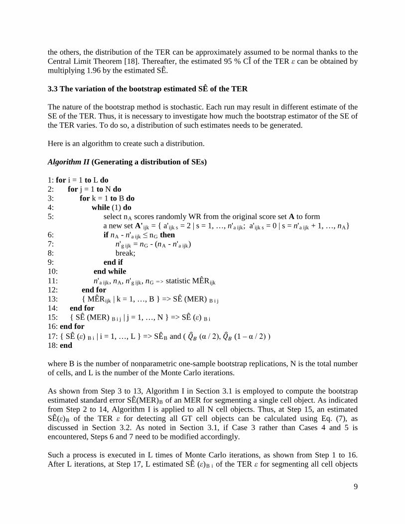
the others, the distribution of the TER can be approximately assumed to be normal thanks to the Central Limit Theorem [18]. Thereafter, the estimated 95 % CÎ of the TER ε can be obtained by multiplying 1.96 by the estimated SÊ. 3.3 The variation of the bootstrap estimated SÊ of the TER The nature of the bootstrap method is stochastic. Each run may result in different estimate of the SE of the TER. Thus, it is necessary to investigate how much the bootstrap estimator of the SE of the TER varies. To do so, a distribution of such estimates needs to be generated. Here is an algorithm to create such a distribution. Algorithm II (Generating a distribution of SEs) 1: for i = 1 to L do 2: for j = 1 to N do 3: for k = 1 to B do 4: while (1) do 5: select nA scores randomly WR from the original score set A to form a new set A'ijk = { a'ijk s = 2 | s = 1, …, n'a ijk; a'ijk s = 0 | s = n'a ijk + 1, …, nA} 6: if nA - n'a ijk ≤ nG then 7: n'g ijk = nG - (nA - n'a ijk) 8: break; 9: end if 10: end while 11: n'a ijk, nA, n'g ijk, nG => statistic MÊRijk 12: end for 13: { MÊRijk | k = 1, …, B } => SÊ (MER) B i j 14: end for 15: { SÊ (MER) B i j | j = 1, …, N } => SÊ (ε) B i 16: end for 17: { SÊ (ε) B i | i = 1, …, L } => SÊB and ( 𝑄�𝐵 (α / 2), 𝑄�𝐵 (1 – α / 2) ) 18: end where B is the number of nonparametric one-sample bootstrap replications, N is the total number of cells, and L is the number of the Monte Carlo iterations. As shown from Step 3 to 13, Algorithm I in Section 3.1 is employed to compute the bootstrap estimated standard error SÊ(MER)B of an MER for segmenting a single cell object. As indicated from Step 2 to 14, Algorithm I is applied to all N cell objects. Thus, at Step 15, an estimated SÊ(ε)B of the TER ε for detecting all GT cell objects can be calculated using Eq. (7), as discussed in Section 3.2. As noted in Section 3.1, if Case 3 rather than Cases 4 and 5 is encountered, Steps 6 and 7 need to be modified accordingly. Such a process is executed in L times of Monte Carlo iterations, as shown from Step 1 to 16. After L iterations, at Step 17, L estimated SÊ (ε)B i of the TER ε for segmenting all cell objects

10

are generated, and they constitute a distribution. Thereafter, the estimated SÊB and 95 % CÎ (𝑄�𝐵 (α / 2), 𝑄�𝐵 (1 – α / 2)) of the distribution of the SÊ (ε)B of the TER can be computed. While estimating the (1 - α) 100% CI at the significance level α, the estimators of the α/2 100% and (1 - α/2) 100% quantiles of the distribution are calculated using the Definition 2 of quantile in Ref. [19]. That is, the sample quantile is obtained by inverting the empirical distribution function with averaging at discontinuities. If 95% CÎ is of interest, then α is set to be 0.05. Finally, the number of the Monte Carlo iterations L needs to be determined. Based on our previous studies, to create a stable distribution, it is enough that the repeated process described above be executed 500 times, i.e., L = 500 [3, 5]. 4 An analytical method for computing the uncertainty of the TER As far as the average MER ra with equal weight ½, as shown in the first formula of Eq. (3), is concerned, its SE may be estimated analytically, since the correlation between the FN rate rfn and the FP rate rfp in the CIS application can be easily calculated. In the majority of cases in the CIS databases, the numbers of pixels in three regions, i.e., the intersection region, the FN region, and the FP region, are five or more, respectively. In other words, both conditions np ≥ 5 and n(1-p) ≥ 5, where n = nG and p = rfn, or n = nA and p = rfp, are satisfied. Thus, in virtue of the central limit theorem, the sampling distribution of the sample FN rate and the sampling distribution of the sample FP rate can all be approximated by a normal probability distribution [18]. As a result, the estimated SÊs of the FN rate rfn and the FP rate rfp, defined as the standard deviation of the sample proportion, can be computed using

SE� = ��̂� (1 − �̂�)

𝑛 (8)

where �̂� = rfn and n = nG for SÊfn, and �̂� = rfp and n = nA for SÊfp. With respect to a GT cell object and its related AD cell object, assuming they are not separated, if the size of the FN region increases (or decreases) by one pixel, then the size of the FP region also increases (or decreases) by one pixel accordingly. In other words, if the FN rate rfn changes by 1 / nG positively or negatively, then the FP rate rfp changes by 1 / nA positively or negatively as well. Thus, intuitively, the correlation between the FN rate rfn and the FP rate rfp is a perfect positive linear. In other words, the correlation coefficient between these two rates in the particular CIS application is 1. The detailed proof is given in the Appendix. As a result, the estimated SÊa of the average MER ra for segmenting a single GT cell object is

SE�a = SE�fn + SE�fp

2 . (9)

11

Finally, the estimated variance of the TER ε for segmenting all GT cell objects can be obtained by replacing SÊB i with the analytically estimated SÊa i of the average MER for detecting the i-th single cell in Eq. (7). Its square root is the estimated SÊ of the TER ε. Subsequently, the estimated 95 % CÎ of the TER ε is obtained by adding and subtracting 1.96 times the estimated SÊ. The analytical approach is a deterministic process. Thus, there is no need to run it multiple times. 5 Results

Figure 3 The histogram of the sizes of all 106 GT cells.

The dataset employed in this article consisted of 106 cells with different sizes, which were manually segmented as GT cell objects [2]. Fig. 3 shows the histogram of sizes of all these 106 GT cell objects in terms of the total number of pixels covered by the GT cell object. The sizes of GT cell objects ranged from 647 up to 27 562 pixels. The median size was 5 368 pixels, and the mean value was 6 062 pixels. The distribution of the sizes of GT cells was skewed on the right side. The variation of sizes of the GT cells was quite large. Therefore, the sizes of the cells must be taken into account while designing the measure in the evaluation of the CIS algorithms. Further, the seven CIS algorithms taken from the ImageJ as described in Section 1 were employed to segment all cell objects. If a CIS algorithm detects a GT cell object with a completely separated AD cell object, both FN rate rfn and FP rate rfp equal one and thus the estimated SÊ of the MER is zero. This can lower the estimation of the SE of the TER for detecting all GT cell objects. Among all seven CIS algorithms employed in this article, Algorithm 4 had one such case and Algorithm 7 had four such cases. In Table 1 are shown the estimated TÊRs, SÊs and 95 % CÎs of TER for seven CIS algorithms. When the weighted MER was used in TER, only the bootstrap method was employed; when the average MER was used, both the bootstrap method and the analytical method were employed. In Figure 4 are depicted the estimated TÊRs and their 95 % CÎ for all seven CIS algorithms computed using the bootstrap method applied to the average MERs. It is the same as shown in our previous studies that the TER computed using the weighted MER is generally larger than the one calculated using the average MER [2]. For four Algorithms 1, 3,

12

5, and 6, the estimated SÊs computed using the weighted MERs are compatible with those using the average MERs for the bootstrap method in terms of the magnitude. The SÊs estimated using the analytical method are generally smaller than those estimated using the bootstrap method.

Alg’s TÊR, SÊ and 95 % CÎ of TER

Weighted MER Average MER Bootstrap Bootstrap Analytical Method

1 0.057524 0.000895

(0.055770, 0.059278)

0.035842 0.000977

(0.033928, 0.037756)

0.035842 0.000169

(0.035510, 0.036174)

2 0.066889 0.000093

(0.066708, 0.067071)

0.037330 0.000246

(0.036848, 0.037813)

0.037330 0.000181

(0.036976, 0.037685)

3 0.089363 0.000666

(0.088058, 0.090669)

0.046528 0.000529

(0.045491, 0.047566)

0.046528 0.000180

(0.046176, 0.046881)

4 0.105096 0.000061

(0.104976, 0.105215)

0.058023 0.000254

(0.057525, 0.058520)

0.058023 0.000188

(0.057654, 0.058392)

5 0.171153 0.001723

(0.167775, 0.174531)

0.086210 0.001908

(0.082471, 0.089950)

0.086210 0.000196

(0.085826, 0.086594)

6 0.173513 0.000878

(0.171791, 0.175235)

0.087080 0.000815

(0.085482, 0.088678)

0.087080 0.000219

(0.086651, 0.087509)

7 0.224444 0.000096

(0.224255, 0.224632)

0.127707 0.000292

(0.127134, 0.128279)

0.127707 0.000208

(0.127300, 0.128114) Table 1 The estimated TÊRs, SÊs and 95 % CÎs of TER for seven CIS algorithms. When the weighted MER was used in TER, only the bootstrap method was employed; when the average MER was used, both the bootstrap method and the analytical method were employed.

Figure 4 The estimated TÊRs and their 95 % CÎ of seven CIS algorithms computed using the bootstrap method while the average MERs were employed.

13

It is known that the Z score corresponding to 95 % CI is 1.96. Thus, in terms of the relative error defined as “1.96 x SÊ / TÊR”, its range is between 0.08 % and 3.05 % for the bootstrap method using the weighted MERs; between 0.45 % and 5.34 % for the bootstrap method using the average MERs; and between 0.32 % and 0.95 % for the analytical method using the average MERs. Taking Algorithm 1 as an example, the three relative errors are 3.05 %, 5.34 %, and 0.93 %, respectively.

Algorithms Mean, SÊ (relative error) and 95 % CÎ of distribution of SÊs of TÊR

Weighted MER Average MER

1 0.000903

0.000007 (1.47 %) (0.000890, 0.000916)

0.000992 0.000012 (2.38 %)

(0.000971, 0.001017)

2 0.000093

0.000000 (0.57 %) (0.000092, 0.000093)

0.000247 0.000000 (0.38 %)

(0.000246, 0.000248)

3 0.000668

0.000006 (1.87 %) (0.000657, 0.000682)

0.000535 0.000007 (2.63 %)

(0.000522, 0.000549)

4 0.000061

0.000000 (0.99 %) (0.000060, 0.000061)

0.000253 0.000001 (0.39 %)

(0.000253, 0.000254)

5 0.001712

0.000012 (1.36 %) (0.001689, 0.001735)

0.001902 0.000018 (1.88 %)

(0.001866, 0.001937)

6 0.000874

0.000006 (1.36 %) (0.000863, 0.000886)

0.000818 0.000009 (2.20 %)

(0.000801, 0.000836)

7 0.000096

0.000000 (0.97 %) (0.000095, 0.000097)

0.000291 0.000001 (0.43 %)

(0.000290, 0.000293) Table 2 The estimated means, SÊs (relative errors) and 95 % CÎs of distributions of the bootstrap estimated SÊs of TÊR for seven CIS algorithms, calculated for the weighted MER and the average MER.

Figure 5 The histograms of SEs of the bootstrap estimated TÊR using weighted MERs (1) and average MERs (2), respectively, for four CIS Algorithms 1 (blue), 3 (red), 5 (green), and 6 (gray). The black circle stands for the estimated mean of the distribution.

14

Under the same circumstances regarding the computation method and the MER employed, the estimated 95 % CÎs of some algorithms do not overlap; but some of them do overlap, as shown in Table 1. These phenomena are manifested in Figure 4. For instance, Algorithm 1’s 95 % CÎ overlaps Algorithm 2’s, but does not overlap Algorithm 3’s. This shows that the performance of Algorithm 1 is obviously better than the performance of Algorithm 3. However, the hypothesis testing is needed to determine the statistical significance of the performance difference between Algorithm 1 and Algorithm 2 even though the estimated TÊR of Algorithm 1 is smaller than the one of Algorithm 2 [3]. As emphasized above, the nature of the bootstrap method is stochastic. Hence, the Algorithm II presented in Section 3.3 was used to generate a distribution of estimated SÊ of TER for a CIS algorithm computed using the bootstrap method. In Table 2 are shown the estimated means, SÊs (relative errors) and 95 % CÎs of distributions of the bootstrap estimated SÊs of TÊR for seven CIS algorithms, calculated for the weighted MER and the average MER. Here the relative error defined as “1.96 x SE / mean” rather than the relative SE defined as “SE / mean” is adopted. In such a way, it can take account of all estimators occurring in the estimated 95 % CÎ, and thus it can describe the stochastic nature of the bootstrap more accurately, namely, how much the bootstrap estimated SÊ of TER can vary. As shown in Table 2, all estimated 95 % CÎs of the bootstrap estimated SÊs of TER are quite narrow. The largest relative error is 2.63 %. In other words, although every time the bootstrap estimated SÊs of TER are different, but they will not be beyond 2.63 % of the estimated mean value of SEs. In Figure 5 are depicted the histograms of the bootstrap estimated SÊs of TER using weighted MERs (1) and average MERs (2), respectively, for four CIS Algorithms 1 (blue), 3 (red), 5 (green), and 6 (gray), the relative errors of which are all greater than 1.00 %. The black circle stands for the estimated mean of the distribution. It shows that the widths of all distributions are very narrow, which indicates that all estimated 95% CÎ are small and demonstrates that the bootstrap results are quite stable. It is worth mentioning that in Table 1, all estimated SÊs of TER calculated using the bootstrap method were obtained by a random execution of a stochastic process, for both weighted MER and average MER. However, they all correspondingly fall in the estimated 95 % CÎ of the bootstrap estimated SÊs of TER that were shown in Table 2. 6 Conclusions and discussion In molecular biology and cellular biochemistry, the data analysis of CIS is fundamentally important regarding segmenting cells in fluorescent microscopy images. In order to evaluate and compare the performance levels of different segmentation algorithms, not only does a measure of performance levels of algorithms need to be developed, but the uncertainty of measure needs to be quantified.

15

In this article, the TER ε, which aggregates all cell objects’ MERs statistically to be a weighted sum using the sizes of the cell objects as weights, is defined as the measure in CIS. Such a formation of a measure in the CIS data analysis can ensure that the penalties for misclassifying cells are proportional to the sizes of cells. In order to quantify the uncertainties of the TER, both the nonparametric bootstrap method based on our extensive research in biometrics and the analytical method were employed. As discussed in Section 1, the CIS application is different compared to the biometrics applications. Thus, the bootstrap method applied in this article was modified accordingly. As discussed in Section 3.1, when a GT cell object and its associated AD cell object are either completely separated or completely overlapped, the estimated SÊ is assumed to be 0. This assumption can be justified by using the analytical formulas shown in Section 4. Certainly, the chance of occurrence of these two cases is rare. For the weighted MER, it is hard to calculate the covariance term analytically so as to estimate the uncertainty of the measure TER in CIS. Hence, only the nonparametric bootstrap method was used for the weighted MER, but both bootstrap method and analytical method were used for the average MER. As far as the measure is concerned, the weighted MER is more conservative than the average MER [2]. But as shown in Table 1 of Section 5, the estimated SÊs of the TERs using weighted MERs are not as consistent as those using average MERs in terms of the magnitudes of the estimated SÊs. For instance, those generated by Algorithms 2, 4, and 7 are relatively small. This may be caused by the complicated formation of the weighted MER. Also as presented in Table 1 of Section 5, the SÊs estimated using the analytical method are generally smaller than those estimated using the bootstrap method. This may be caused by the fact that there exist some cases in the CIS databases where the normality conditions are not satisfied. In addition, the estimated SÊ expressed by Eq. (8) does not take account of the interrelationship between the two distributions shown in Figure 2 [3, 21]. As a consequence and to be more conservative, the nonparametric bootstrap method is recommended over the analytical method for estimating the uncertainties of the TER in CIS. The nature of the bootstrap method is stochastic. The variation of the bootstrap estimated SÊ of the TER was investigated. The distributions of the bootstrap estimated SÊs of TER in CIS were generated using the Algorithm II in Section 3.3, and evaluated in Section 5. All estimators of related 95 % CÎs are quite narrow. Although they are different each time, the bootstrap estimated SÊs of TER are not beyond 2.63 % of the estimated mean value of SEs in our examples. Moreover, in our studies, all bootstrap estimators of SÊs of TER obtained by a random execution of a stochastic process, regardless of whether the weighted MER or the average MER was employed, fall correspondingly in the estimated 95 % CÎ of the bootstrap estimated SÊs of TER. As shown in Table 1 and Figure 4, the estimated 95 % CÎs of some CIS algorithms do not overlap; but some of them do overlap, under the same circumstances regarding the computation method and the MER employed. In the former cases, it is easy to reach the conclusion about

16

which algorithm’s performance is better. However, in the latter cases, the hypothesis testing needs to be subsequently carried out in order to determine the statistical significance of the performance differences. Then, the correlation coefficient between the two algorithms’ TERs also needs to be computed [3, 20].

Appendix For a GT cell object and its corresponding AD cell object, assuming they are not separated, once the size of the FN region increases or decreases by one pixel, the size of the FP region will increase or decrease by one pixel as well. Using the notations in Section 2, the correlated pairs of the FN rate rfn and the FP rate rfp can be expressed by

� 𝑟fn 𝑖, 𝑟fp 𝑖 � = � 𝑛g + 𝑖𝑛G

,𝑛a + 𝑖𝑛A

� , 𝑖 = −𝑚, … ,−1, 0, 1, … ,𝑛 (A1)

where the constraints are ng – m ≥ 0, na – m ≥ 0, ng + n ≤ nG, na + n ≤ nA, and nG – ng = nA – na. The averages of the FN rate and the FP rate are, Finally, the correlation coefficient is,

𝜌 =∑ ( 𝑟fn 𝑖 − �̅�fn ) ( 𝑟fp 𝑖 − �̅�fp )𝑛𝑖= −𝑚

�∑ ( 𝑟fn 𝑖 − �̅�fn )2𝑛𝑖 = −𝑚 �∑ ( 𝑟f𝑝 𝑖 − �̅�f𝑝 )2𝑛

𝑖 = −𝑚

= ∑ � 𝑖 − 𝑛 −𝑚

2 � � 𝑖 − 𝑛 −𝑚2 �𝑛

𝑖 = −𝑚

�∑ ( 𝑖 − 𝑛 −𝑚2 )2𝑛

𝑖 = −𝑚 �∑ ( 𝑖 − 𝑛 −𝑚2 )2𝑛

𝑖 = −𝑚

= 1 . (A3)

References

1. K. Wu, D. Gauthier and M.D. Levine, Live cell image segmentation, IEEE Trans. on Biomedical Engineering 42 (1), 1-12 (1995).

2. J.C. Wu, M. Halter, R.N. Kacker and J.T. Elliott, A new measure in cell image segmentation data analysis, NISTIR 7871, National Institute of Standards and Technology, July, (2012).

�̅�fn = 1

𝑚 + 𝑛 + 1 �

𝑛g + 𝑖𝑛G

𝑛

𝑖 = −𝑚

= 𝑛g𝑛G

+ 1𝑛G

× 𝑛 −𝑚

2

(A2) �̅�fp =

1𝑚 + 𝑛 + 1

�𝑛a + 𝑖𝑛A

𝑛

𝑖 = −𝑚

= 𝑛a𝑛A

+ 1𝑛A

× 𝑛 −𝑚

2 .

17

3. J.C. Wu, A.F. Martin and R.N. Kacker, Measures, uncertainties, and significance test in operational ROC analysis, J. Res. Natl. Inst. Stand. Technol. 116 (1), 517-537 (2011).

4. J.C. Wu, A.F. Martin, C.S. Greenberg and R.N. Kacker, Data dependency on measurement uncertainties in speaker recognition evaluation, in Active and Passive Signatures III, Proc. SPIE Vol. 8382, 83820D (2012).

5. J.C. Wu, A.F. Martin and R.N. Kacker, Bootstrap variability studies in ROC analysis on large datasets, Communications in Statistics - Simulation and Computation, in press, (2013).

6. P. Jaccard, Distribution de la flore alpine dans le bassin des Dranses et dans quelques régions voisines, Bulletin de la Société Vaudoise des Sciences Naturelles 37, 241-272 (1901).

7. W.M. Rand, Objective criteria for the evaluation of clustering methods, Journal of the American Statistical Association, 66 (336), 846–850 (1971).

8. A.P. Zijdenbos, B. M. Dawant, R.A. Margolin and A.C. Palmer, Morphometric Analysis of White Matter Lesions in MR Images: Method and Validation, IEEE Trans. Medical Imaging, 13 (4), 716- 724 (1994).

9. F. Yang, M.A. Mackey, F. Ianzini, G. Gallardo and M. Sonka, Cell Segmentation, Tracking, and Mitosis Detection Using Temporal Context, in J. Duncan and G. Gerig (Eds.): MICCAI 2005, LNCS 3749, 302-309 (2005).

10. L.P. Coelho, A. Shariff and R.F. Murphy, Nuclear segmentation in microscope cell images: A hand-segmented dataset and comparison of algorithms, in Proc IEEE Int Symp Biomed Imaging, 518–521 (2009).

11. J. Strijbos, R. Martens, F. Prins and W. Jochems, Content analysis: What are they talking about? Computers & Education, 46, 29–48 (2006).

12. D.J. Hand, Construction and assessment of classification rules, John Wiley & Sons, New York, (1997).

13. “NIST Semantics for Biological Data Resource: Cell Image Database”, National Institute of Standards and Technology, http://sbd.nist.gov/, (2013).

14. Rasband, W.S., ImageJ, U. S. National Institutes of Health, Bethesda, Maryland, USA, http://rsbweb.nih.gov/ij/, 1997-2008.

15. B. Efron, Bootstrap methods: Another look at the Jackknife, Ann. Statistics 7, 1-26 (1979).

16. B. Efron and R.J. Tibshirani, An Introduction to the Bootstrap, Chapman & Hall, New York, (1993).

17. B.L. van der Waerden, Mathematical Statistics, Springer, Berlin, (1969). 18. J.A. Rice, Mathematical Statistics and Data Analysis (3rd ed.), Duxbury Advanced,

Belmont, CA, (2006). 19. R.J. Hyndman and Y. Fan, Sample quantiles in statistical packages, American Statistician

50:361-365 (1996). 20. J.C. Wu, A.F. Martin, C.S. Greenberg, R.N. Kacker and V.M. Stanford, Significance test

with data dependency in speaker recognition evaluation, in Active and Passive Signatures IV, Proc. SPIE Vol. 8734, 87340I (2013).

21. K. Linnet, Comparison of quantitative diagnostic tests: type I error, power, and sample size, Statistics in Medicine 6, 147-158 (1987).