measuring and modeling execution cost and...
TRANSCRIPT

Measuring and Modeling Execution Cost and Risk1
Robert Engle NYU and Morgan Stanley
Robert Ferstenberg Morgan Stanley
Jeffrey Russell
University of Chicago [email protected]
January 2008
Abstract: Financial markets are considered to be liquid if a large quantity can be traded quickly and with minimal price impact. Although the idea of a liquid market involves both a cost as well as a time component, most measures of execution costs tend to focus on only a single number reflecting average costs and do not explicitly account for the temporal dimension of liquidity. In reality, trading takes time since larger orders are often broken up into smaller transactions or when limit orders are used. Recent work shows that the time taken to transact introduces a risk component in execution costs. In this setting, the decision can be viewed as a risk/reward tradeoff faced by the investor who can solve for a mean variance utility maximizing trading strategy. We introduce an econometric method to jointly model the expected cost and the risk of the trade thereby characterizing the mean variance tradeoffs associated of different trading approaches given market and order characteristics. We apply our methodology to a novel data set and show that the risk component is a non-trivial part of the transaction decision. The conditional distribution of transaction costs is also used to construct a new measure of liquidation risk that we refer to as liquidation value at risk (LVaR).

2
I. Introduction
Measuring and understanding financial execution costs is important for both practitioners and
regulators and has attracted substantial attention from the academic literature. Markets are
considered to be liquid if a large quantity can be traded quickly and with minimal price impact.
While the idea of a liquid market involves both a cost as well as a time component, most
measures of execution costs tend to focus on only a single number such as bid ask spreads or
realized effective spreads. A recent special issue of the Journal of Financial Markets (2003) gives
a good overview of this literature including careful analysis of some of the important
assumptions. See in particular, Lehmann (2003), Bessimbinder (2003), Werner (2003), Petersen
and Sirri (2003).
Many strategies to reduce execution costs require taking more time to trade. This could be
delaying trades to search for and take advantage of higher liquidity environments, breaking up
trades to reduce spreads and price impact or using more out of the money limit orders. Recent
work by Almgren and Chriss (1999, 2000) and Almgren (2003), and Grinold and Kahn (1999)
point out that this added time to trade corresponds to an added risk of trading, thus introducing a
risk return trade-off in execution itself. They develop families of execution strategies that lie on a
risk return frontier under specific assumptions on the execution technology. More risk averse
agents will trade more rapidly thus incurring higher transaction costs but lower risk. An
execution strategy that takes a substantial risk should be risk adjusted before being compared with
lower risk strategies. Engle and Ferstenberg (2007) embed this problem in a full portfolio
optimization showing that the risk return tradeoff in portfolio theory implies a criterion for
optimizing execution.
We are not aware of any paper that has shown that empirically there is a risk return trade
off in order execution. While it is easy to develop trading algorithms that take more risk, it is not
clear how much reduction in transaction costs, if any, can be achieved by such devices. Partly
this is due to a difficulty in obtaining order data, and partly it is due to a lack of econometric
techniques to simultaneously measure the first two moments of transaction costs.
In this paper we develop empirical measures of the risk and return to trading. This
paper will estimate risk return frontiers for a set of trading strategies. Given estimates of the
conditional risk and return of different trading strategies we can, and do, calculate risk adjusted
costs of execution for investors with a particular tolerance for risk. We also examine the choice

3
of trading strategy for investors with different risk tolerances and find that traders appear to select
trading strategies that imply extreme risk aversion. This suggests that traders are overly risk
averse in selection of their trading strategy.
This paper focuses on single orders, sometimes called parent orders, which are broken up
into a sequence of smaller orders, called child orders. As the parent orders are executed, they
appear in most datasets to be small transactions in a correlated order flow. However, the cost
incurred by the trader is not a function of a single transaction, but rather the entire sequence of
child orders. Perold (1988) introduced “implementation shortfall” as a measure of transaction
costs that can accommodate such parent orders. Implementation shortfall compares the value of a
paper portfolio with no transaction costs to the real portfolio obtained by actual trading. This
measure of execution cost has been used in empirical work by Keim and Madhavan (1997),
Bertsimas and Lo (1998), and Conrad Johnson and Wahal (2003), for example. Importantly,
these studies do not consider risk as we do in our work and therefore miss an important
component of liquidity. They are unable to risk adjust the transaction costs.
Our data consists of a sample of 233,913 orders executed by Morgan Stanley in 2004.
We use this data to construct measures of both execution risk and cost2 conditional on order and
market characteristics.
The paper is organized as follows. Section 2 discusses the choice of trading strategy by
the investor. Section 3 introduces measures of order execution cost and risk. Section 4 presents
the data used in our analysis and some preliminary analysis. Section 5 presents a model for
conditional cost and risk along with estimates while section 6 employs diagnostic tests to develop
a richer specification. Section 7 explicitly examines the economic importance of transaction risk,
section 8 presents an application of the model to liquidity risk and section 9 concludes.
II. Choice of trading strategy
Investors are offered a wide choice of strategies for executing a particular order. The order
can be executed by a block trader from one of many brokerage houses or by algorithmic trading
from many different vendors. Within each of these categories there are a range of options which
might entail some risk sharing with the broker, some specific instructions, some specific venue, a
particular crossing strategy, or many other considerations. Each of these possibilities could give
an estimate of the expected cost and the expected risk of the trade. The investor would then use
2 The data does not include the identities of the traders.

4
an appropriate utility function to determine the best way to execute the trade. It could turn out
that one of the options is not to execute the order at all and this could also be an outcome.
In order to do this optimization, each venue must be associated with a risk and return estimate
for all types of orders. That is, given the name, quantity, day and instructions, what is the
outcome expected to be? Not all venues provide such information. Because this is a repeating
business, however, it is possible for clients to construct their own estimates. This can also be
useful because it gives a way to evaluate the success of brokers in achieving the performance they
advertise.
The building blocks for this decision analysis are the expected cost and risk as a function of a
set of characteristics specific to each venue. It is possible that there will be some characteristics
of an order that are not observable to the econometrician or possibly to the broker. Some orders
may be based on information on upcoming announcements or other forthcoming trades, possibly
from the same investor. These orders might have performance that deviates from the average in
either mean or risk.
If there are important unobserved characteristics of orders, then the function predicting the
mean and variance of transaction cost will inappropriately attribute these trades to correlated
observable characteristics. In particular, these unobservable characteristics could be associated
with trading instructions. For example, if an announcement is expected very soon, then the order
could be called urgent and would be traded fast with less concern for cost. Consequently, orders
labeled urgent may on average have worse execution in either mean or variance than would be
expected given the trading environment. The situation is like errors in variables or simultaneous
equations bias. Although there will be a bias in the coefficients from the structural relation, the
estimated coefficients will still give an unbiased estimate of the conditional expectation, and
perhaps that is the most useful result. This endogeneity has always been present in trade data
and we have hundreds of studies of trade execution that appear to be reliable and reproducible.
Many investors, who issue urgent instructions because they believe they have time sensitive
information, may have less information than they think and consequently are simply paying too
much for their executions. There is evidence in our data set for this position. As in simultaneous
equation estimation, a small endogeneity leads to a small bias. In this paper we will assume that
the unmeasured characteristics of trades are relatively small and uncorrelated with the observable
characteristics, and we interpret the results as the expected costs and risks of a typical trade with
particular characteristics when executed using a certain strategy.

5
III. Measuring order execution cost and risk.
This section defines the transaction cost measure and shows how it relates to the portfolio risk
and return. Let the position measured in shares at time period t be xt . The number of shares
transacted in period t is simply the change in xt so that purchases are positive and sales are
negative. Let 0p denote the fair market value of the asset at the time of the order arrival; in
practice this will be the midquote at the time of the order arrival. Let tp~ denote the transaction
price of the asset in period t which will in general depend upon the size, direction and timing of
the trades. Trading takes place over the time interval [0,T] where x0 denotes the initial position
prior to trade and xT the position post trade. The transaction cost for a given parent order is then
defined to be:
(1) ( )∑=
−Δ=T
ttt ppxTC
10
~
Notice that this is simply the cost of acquiring ( )0Tx x− shares with actual transaction prices
minus the cost of acquiring these shares at the initial fair market price of p0. Transactions that
occur above the reference price will therefore contribute positively toward transaction costs when
purchasing shares. Alternatively, when liquidating shares, the change in shares will be non-
positive, hence transaction prices that occur below the reference price will contribute positively to
transaction costs. For a given order, the transaction costs can be either negative or positive
depending upon whether the price moved with or against the direction of the order. However,
because each trade has a price impact that tends to move the price up for buys and down for sells,
we would expect the parent transaction cost to be positive on average. This transaction cost is
the realization of a random variable with both a mean and variance that can be estimated. A
measure of the transaction cost per dollar traded is obtained by dividing the transaction cost by
the arrival value:
(2) 0 0
%T
TCTCx x p
=−
This measure allows for more meaningful comparison of execution cost for different stocks with
different prices and therefore serves as the basis of our empirical work.
Engle and Ferstenberg (2007) further show that the change in portfolio value, yt, over this
period can be expressed as
(3) ( )0 0'T T Ty y x p p TC− = − −
6
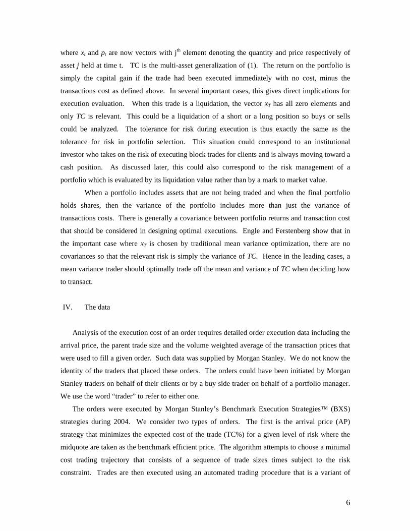
where xt and pt are now vectors with jth element denoting the quantity and price respectively of
asset j held at time t. TC is the multi-asset generalization of (1). The return on the portfolio is
simply the capital gain if the trade had been executed immediately with no cost, minus the
transactions cost as defined above. In several important cases, this gives direct implications for
execution evaluation. When this trade is a liquidation, the vector xT has all zero elements and
only TC is relevant. This could be a liquidation of a short or a long position so buys or sells
could be analyzed. The tolerance for risk during execution is thus exactly the same as the
tolerance for risk in portfolio selection. This situation could correspond to an institutional
investor who takes on the risk of executing block trades for clients and is always moving toward a
cash position. As discussed later, this could also correspond to the risk management of a
portfolio which is evaluated by its liquidation value rather than by a mark to market value.
When a portfolio includes assets that are not being traded and when the final portfolio
holds shares, then the variance of the portfolio includes more than just the variance of
transactions costs. There is generally a covariance between portfolio returns and transaction cost
that should be considered in designing optimal executions. Engle and Ferstenberg show that in
the important case where xT is chosen by traditional mean variance optimization, there are no
covariances so that the relevant risk is simply the variance of TC. Hence in the leading cases, a
mean variance trader should optimally trade off the mean and variance of TC when deciding how
to transact.
IV. The data
Analysis of the execution cost of an order requires detailed order execution data including the
arrival price, the parent trade size and the volume weighted average of the transaction prices that
were used to fill a given order. Such data was supplied by Morgan Stanley. We do not know the
identity of the traders that placed these orders. The orders could have been initiated by Morgan
Stanley traders on behalf of their clients or by a buy side trader on behalf of a portfolio manager.
We use the word “trader” to refer to either one.
The orders were executed by Morgan Stanley’s Benchmark Execution Strategies™ (BXS)
strategies during 2004. We consider two types of orders. The first is the arrival price (AP)
strategy that minimizes the expected cost of the trade (TC%) for a given level of risk where the
midquote are taken as the benchmark efficient price. The algorithm attempts to choose a minimal
cost trading trajectory that consists of a sequence of trade sizes times subject to the risk
constraint. Trades are then executed using an automated trading procedure that is a variant of

7
Almgren and Chriss (2000). The second is a volume weighted average price strategy. This
strategy attempts to trade as close as possible to the volume weighted average price over a
specified time interval.
For the AP strategy, the trader chooses one of three urgency levels - high, medium, and
low. The level of urgency is inversely related to the level of risk that the trader is willing to
tolerate. High urgency orders have relatively low risk, but execute at a higher average cost
obtained by trading very quickly. The medium and low urgency trades execute with
progressively higher risk but at a lower average cost obtained by trading more slowly, over a
longer period of time. The trader chooses the urgency and the algorithm derives the time to
complete the trade given the state of the market and the trader’s constraints. Given order size and
market conditions, lower urgency orders tend to take longer to complete than higher urgency
trades. However, since the duration to completion depends upon the market conditions and other
factors, there is not perfect correspondence between the urgency level and the time to complete
the order. All orders in our sample, regardless of urgency, are filled within a single day.
For VWAP strategies, the trader selects a time horizon and the algorithm attempts to
execute the entire order by trading proportional to the market volume over this time interval. We
only consider VWAP orders where the trader directed that the order be filled over the course of
the entire trading day or that the overall volume traded was a very small fraction of the market
volume over that period. This can be interpreted as a strategy to minimize cost regardless of risk.
As such, we consider this a risk neutral trading VWAP strategy. This need not correspond to a
risk neutral strategy, but clearly the intent of the trader is consistent with risk neutral VWAP
trading. Generally, these orders take longer to fill than the low urgency orders and should
provide the highest risk and the lowest cost.
We consider orders for both NYSE and Nasdaq stocks. Several filters are applied to our
transaction data. We only consider completed orders. Hence orders that begin to execute and are
then cancelled midstream are not included in order to ensure homogeneity of orders of a given
type. We excluded short sales because the uptick rule prevents the economic model from being
used "freely". We do not consider orders executed prior to 9:36 since the market conditions
surrounding the open are quite different than non-opening conditions. Only stocks that have an
arrival price greater than $5 are included – we find that very cheap stocks have transaction prices
that are impacted by price discreteness and may require special modeling techniques appropriate
for such data. Orders that execute in less than 5 minutes tend to be very small orders that may be
traded in a single trade and are not representative of the mean variance tradeoff that is of interest
in our work. For similar reasons, orders smaller than 1000 shares are also not included. Finally,

8
orders that are constrained to execute more quickly than the algorithm would dictate due to the
approaching end of the trading day are also excluded. In the end, we are left with 233,913 parent
orders.
For each order we construct the following statistics. The percent transaction costs are
constructed using equation (2). We further construct the 5 day lagged bid-ask spread weighted by
time as a percent of the midquote, the annualized 21 day lagged close to close volatility and the
order shares divided by the lagged 21 day median daily volume. Table 1 presents summary
statistics of our data. The statistics weight each order by its fraction of dollar volume.
The rows labeled B and S break down the orders into buyer and seller orders respectively.
62% of the dollars traded were buys and 38% sells. Buy orders tend to be slightly more
expensive on average in this sample. The risk is similar. We see that 75% of the dollar volume
was for NYSE stocks and 25% for Nasdaq. We see that NYSE orders tend to cost less than
Nasdaq by an average of about 5 basis points. It is important to note that these statistics are
unconditional and do not control for differences in characteristics of the stocks traded on the two
exchanges which might be driving some of the variation in the observed costs. For example, we
see that the average volatility of Nasdaq stocks is substantially higher than that of NYSE.
The last four rows separate the orders by urgency. H, M, and L, correspond to high,
medium and low urgencies and V is the VWAP strategy. Hence as we move down the rows we
move from high cost, low risk strategies to low cost, high risk strategies. Almost half of the
orders are the risk neutral VWAP strategy (46%). Only 10% of the order volume is high urgency,
24% is medium urgency and 20% is high urgency. This is reflected in the sample statistics. The
average cost decreases from 11.69 basis points to 8.99 basis points as we move from high to low
urgency orders. At the same time, the risk moves from 12.19 basis points up to 40.89 basis points
for the same change in urgency. Contrary to the intent, the VWAP strategy does not exhibit the
lowest cost at 9.69 basis points. It is the most risky however. Of course, the order submission
may depend on the state of the market and characteristics of the order. These unconditional
statistics will not reflect the market state and may blur the tradeoffs faced by the traders.
Table 2 presents the same summary statistics conditional on the size of the order relative
to the 21 day median daily volume. The first bin is for orders less than a quarter of a percent of
the 21 day median daily volume and the largest bin considered is for orders that exceed 1%. For
each bin the statistics are presented for each type of order. The top of the table is for NYSE and
the bottom half of the table is for Nasdaq stocks. Not surprisingly, for each order type, larger
order sizes tend to be associated with higher average cost and higher risk indicating that larger
orders are more difficult to execute along both the cost and risk dimensions.
9
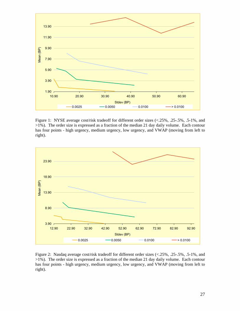
This tradeoff can be seen clearly by plotting the cost/risk tradeoffs for each of the percent
order size bins. Figure 1 presents the average cost/risk tradeoff for the NYSE stocks. Each
contour indicates the expected cost/risk tradeoff faced for a given order size. Each contour is
constructed using 4 points, the three urgencies and the VWAP. For a given contour, as we move
from left to right we move from the high urgency orders to the VWAP. Generally speaking, the
expected cost falls as the risk increases. This is not true for every contour, however. Increasing
the percent order size shifts the entire frontier toward the north east indicating a less favorable
average cost / risk tradeoff. Figure 2 presents the same plot but for Nasdaq stocks.
Contrary to what might be expected, some order size bins exhibit a cost increase as we move
to less urgent strategies. These plots, however, do not consider the state of the market at the time
the order is executed. It is entirely possible that the traders consider the state of the market when
considering what type of urgency to associate with their order. If this is the case, a more accurate
picture of the tradeoff faced by the trader can be obtained by considering the conditional frontier.
This requires building a model for the expected cost and the standard deviation of the cost
conditional on the state of the market and is the goal of the next section of the paper.
V. Modeling the expected cost and risk of order execution.
Both the transaction cost and risk associated with executing a given order will vary according
to characteristics of the order and the state of the market. In this section we propose a modeling
strategy for both the expected cost and risk of trading an order. In this way, we build a model for
the conditional mean variance tradeoff obtained by each trading strategy. The model is estimated
using the Morgan Stanley execution data described in the previous section.
We now propose a joint model for the conditional mean and variance of transaction costs.
Both the mean and the variance of transaction costs are assumed to be an exponential function of
the market variables and the order size. Specifically the transaction costs for the ith order are
given by:
(4) ( ) 1% exp exp2i i i iTC X Xβ γ ε⎛ ⎞= + ⎜ ⎟
⎝ ⎠
where )1,0( ~ Niidiε . The conditional mean is an exponential function of a linear combination
of the Xi with parameter vector β. The conditional standard deviation is also an exponential
function of a linear combination of the Xi with parameter vector γ. Xi is a vector of conditioning

10
information. In our empirical work we find that the same vector Xi explains both the mean and
the variance but this restriction is obviously not required.
Clearly the variance must be a positive number and while the realization of transaction
costs can be either positive or negative (and empirically we do find both signs), the expected
transaction cost should be positive. The exponential specification for both the mean and the
variance restricts both to be positive numbers.
We consider several factors that market microstructure theory predicts should contribute
to the ease/cost of executing a given order. The lagged 5 day time weighted average spread as a
percent of the midquote. The daily volatility constructed from the average close to close returns
over the last 21 days. The average historical 21 day median daily dollar volumes. In addition to
these market variables we also condition on the log of the dollar value of the order and the
urgency associated with the order. The urgency is captured by 3 dummy variables for high,
medium, and low urgencies. The constant term in the mean and variance models therefore
corresponds to the VWAP strategy.
The exponential specification for the mean with an additive disturbance, is not a model
we have seen previously used in the literature. The often used method of modeling the logarithm
of the left hand side variable won’t work here because the transaction cost often takes negative
values. Despite the exponential form for the mean and variance, interpretation of the parameters
is straight forward. Notice that ( )[ ] βii XTCE =%ln . Hence the coefficients can be interpreted
as the percent change in expected TC% for a one unit change in X. Coefficients of right hand
side variables that are expressed as the logarithm of a variable (such as ln(value)) can be
interpreted as the elasticity with respect to the non-logged variable (such as value).
The exponential model also allows for interesting nonlinear interactions that we might
suspect should be present. Consider the expected transaction cost and the logged value (dollar
size of the trade) and volatility variables. We have
( ) ( ) 21ablesother variexp% ββ volatilityvalueTCE = . If 1β is larger than 1 then the cost increases more
than proportionally to the value. If 1β is smaller than 1 then the expected cost increases less than
proportionally to the value. If 1β and 2β are both positive, then increases in the volatility result
in larger increases in the expected cost for larger value trades. Alternatively, as the value of the
trade goes to zero, so does the expected cost which seems reasonable. It is entirely possible that
the marginal impact of volatility might be different for different order sizes. The exponential
model allows for this possibility in a very parsimonious fashion. Hence, what appears as a very
11
simple nonlinear transformation allows for fairly rich nonlinear interactions. Obviously, using
the exponential function for the variance has the same interpretation.
We estimate the model by maximum likelihood under the normality assumption forε . It is
well known that under standard regularity conditions the normality assumption delivers a quasi
maximum likelihood estimator. As long as the conditional mean and variance are correctly
specified, we still obtain consistent estimates of the parameters even if the normality assumption
is not correct. The standard errors, however, will not be correct in the event that the errors are not
normal. Robust standard errors that are consistent in the event of non-normal errors can be
constructed following White (1982) and are constructed for our parameter estimates. The
information matrix is block diagonal between the parameters of the mean and the parameters of
the variance, hence the estimated parameters for the mean and variance equations are
asymptotically independent.
VI. Empirical Results
The estimation is performed separately for NYSE and Nasdaq stocks. The two markets
operate in a very different fashion and it is unlikely a single model would be appropriate for both
trading venues. We have 166,508 NYSE orders and 67,405 Nasdaq orders. We do not separate
VWAP and AP orders, however we will use the order type in the conditioning information set.
We find that empirically this seems reasonable.
We begin by estimating a simple, parsimonious model that allows for particularly easy
interpretation and comparison across NYSE and Nasdaq models. The model uses the same
explanatory variables for both the mean and the variance. Although this simple model actually
performs quite well, we later consider more elaborate models that can extract richer information
about differences between Nasdaq and NYSE order execution.
The simple model contains the spread, the logarithmic daily volatility, the logarithmic
volume, indicator variables for the urgency of the trade and a VWAP indicator variable.
Estimation results for the variance and mean equations for NYSE transactions are given in given
in tables 3 and 4 respectively. Tables 5 and 6 present the model estimates for Nasdaq
transactions.
The estimated coefficients are remarkably similar for the NYSE and Nasdaq models. The
spread coefficient is positive in both the mean and variance equations. Since higher spreads tend
to be associated with less liquid markets it is not surprising to find that wider spreads are
associated with both higher risk and cost - more difficult orders. It is also interesting to see that
12
the coefficient on the spread in the expected cost equations is nearly 1 for both NYSE and Nasdaq
orders. This indicates that, all else equal, if the spread doubles, so does the expected cost – not a
surprising result. Higher volatility stocks are more costly to transact in and, not surprisingly,
have higher risk. In fact, we see that the coefficient on the log volatility is nearly one. Recall that
the model is specified in terms of the transaction cost variance, not volatility (standard deviation).
This implies that the coefficient on the traded assets log variance is half the coefficient on its log
volatility.
If the parent order is traded over a fixed time period by trading equal amounts in each
time interval, then we would expect the variance of transaction cost would be proportional to the
variance of the asset variance. This strategy however does not attempt to minimize risk. A more
sophisticated strategy will accelerate trades when the volatility is high thereby shortening
transaction times. Thus we are not surprised to find that transaction cost variance increases less
than proportional with asset variance.
Not surprisingly, the expected transaction costs are an increasing function of the
volatility. In order to maintain a given level of trading risk, orders for higher volatility stocks
must be executed more quickly than low volatility stocks. This shorter execution time induces
higher expected transaction costs.
The value and volume coefficients are roughly of equal magnitude but opposite sign in
both the expected cost and variance equations for both NYSE and Nasdaq. This is not surprising
since the size (value) of the order must be considered relative to the typical daily volume of the
traded asset. The magnitudes and signs of the estimated coefficient imply that it is the ratio of the
order size to the daily volume that is useful in predicting both cost and risk. The estimated
coefficients are all around .5 in magnitude indicating that both the risk and cost increase roughly
in the square root of the order size expressed as a fraction of daily volume.
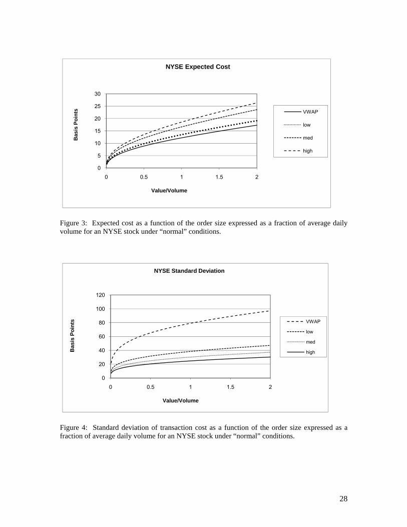
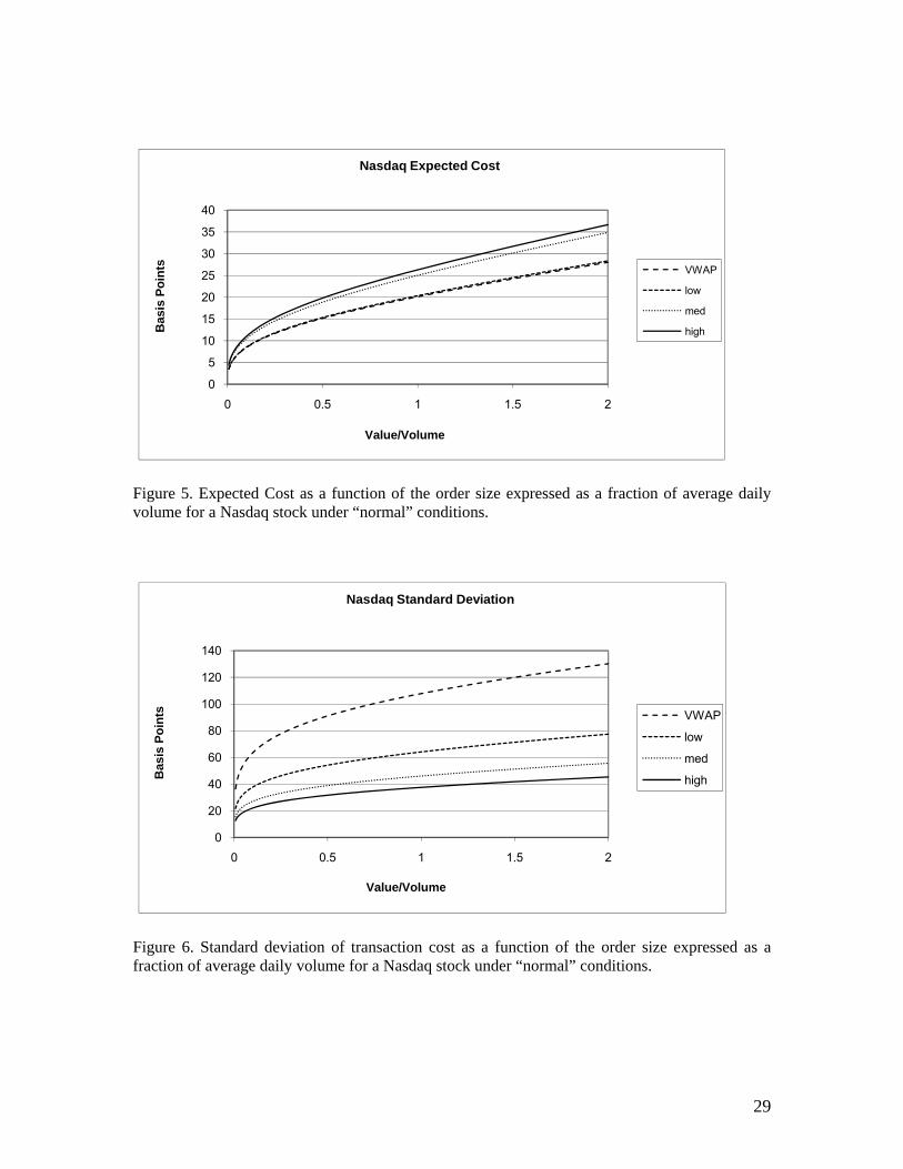
Figures 3 and 4 present the expected cost and the standard deviation (measured in basis
points) of transaction costs as a function of the order size relative to the daily volume.
Normalizing by volume allows us to compare order sizes across stocks with different typical daily
volumes in a more meaningful way. The plots consider order sizes ranging from near 0 percent
up to 2% of the daily volume and represent an average stock on an average day. Figures 5 and 6
present the same plots, but for the Nasdaq stocks. In the expected cost plots, the higher curves
correspond to the more urgent orders. The opposite is true for the standard deviation plots. The
model estimates indicate that both the expected cost and risk are concave functions of the order
size expressed as a fraction of the daily volume. Hence order size increases both expected cost
and variance but at a decreasing rate.

13
The urgency dummy variables appear as expected. We see that the expected cost
increases as the urgency level increases and that the risk decreases with higher urgency orders.
These parameters can be more easily interpreted in the context of the mean variance plots
previously used for the unconditional moments. We again consider the risk/cost tradeoff for an
average stock under average conditions for NYSE and Nasdaq markets. These contours are
plotted in figures 7 and 8. The ellipses represent 95% confidence intervals for the true mean and
true variance for each order submission strategy. As we move from left to right we move from
high urgency to medium, to low and finally VWAP or the risk neutral strategy. The plots suggest
that moving from low urgency to the VWAP strategy tends to increase risk with little reduction in
cost both for NYSE and Nasdaq stocks. We show later in the paper that the VWAP strategy
might be preferred after risk adjusting cost.
We can evaluate the cost/risk tradeoff for the characteristics of any stock and any order
characteristic. To get an idea of how this tradeoff varies as the order size relative to daily volume
varies we next plot the mean variance frontiers for different value ratios. We again consider a
typical stock on a typical day. These plots are presented in figures 9 and 10 for typical NYSE and
Nasdaq stocks respectively. The larger orders shift the cost/risk tradeoff to less desirable north
east region. We again see that the order size effects on the cost/risk tradeoff are substantial.
It is tempting at this point to compare the mean variance frontiers obtained for orders
filled on Nasdaq and orders filled on the NYSE. In doing so, we can compare market quality
using a measurement that reflects real world trading and both expected cost and risk components
of execution cost. We use the estimated models to compare the mean variance frontiers for the
same transaction under identical market conditions on the NYSE and on the Nasdaq. Most
market and order characteristics included in the model are comparable across the two markets
(i.e. volatility is volatility, spreads are spreads). The volume however is not easily comparable
across the two markets. The problem is that much of the volume recorded for Nasdaq trades is
not volume that Morgan Stanley could have participated in. Some trades are directly facilitated
between two dealers in order to rebalance inventories and some of the volume on Nasdaq took
place on satellite markets not available to Morgan Stanley. This is a well known problem and
some estimates put Nasdaq volume at about 30% overstated relative to NYSE. Figure 11 presents
the comparison with no adjustments to the volume. Figure 12 presents the comparison with the
Nasdaq volume 30% greater than the NYSE volume. This adjustment would be the correct if
volume on Nasdaq were in fact 30% overstated as conjectured. Although the NYSE appears to
have lower cost for a given risk level, across all risk levels we see that once the volume
14
differences are accounted for there is little difference between the market qualities implied by our
models.
Finally, despite the similarity in the Nasdaq and NYSE models, we find that the models are
statistically different. We test the null hypothesis that both the mean and variance models are
identical for the NYSE and Nasdaq orders. This null hypothesis is tested by a likelihood ratio test
based on the difference between the sum of the likelihoods for the two unrestricted NYSE and
Nasdaq models and the restricted model using the pooled data. Twice the difference in these two
likelihoods will have a chi-squared distribution with degrees of freedom given by the number of
restricted parameters, or 16. Twice the difference in the two likelihoods is 1954.76. The critical
value is 26.29 so we overwhelmingly reject the null with a p-value near 0. Hence, while the
models are qualitatively similar, there are statistically meaningful quantitative differences.
VII. Specification Tests
This model appears to do a nice job of relating the expected cost and risk components to the
characteristics of the stock traded and the market as well as characteristics of the order. The
parameters are easily interpreted and comparable across models. Nevertheless, specification tests
suggest that more elaborate models could be considered. While the interpretation of the models
may become slightly more complex, more elaborate models might highlight differences between
the NYSE and Nasdaq stocks and more details of how market and order characteristics impact
execution cost and risk.
We considered two extensions of the model, additional nonlinear terms and interactions
between variables. The additional non linear terms considered are the value, volume, volatility
variables in levels (ie not logarithmic) and the logarithmic spread. A natural extension to
consider is that the VWAP orders have different properties than the AP orders. This can be tested
by interacting the VWAP dummy with the variables already considered in the more parsimonious
model presented earlier. This model is the most general we consider and it has many more
variables in both the mean and the variance.
We proceeded to calculate Lagrange Multiplier tests for omitted variables of this general
model. The null model is tested against the general model and if it is rejected, additional
variables are added to the base model until the test fails to reject. In most cases, the variables
with the highest t-statistics in the test are added first.
The LM tests are performed separately on the mean and variance equation for each
market and are easily computed. Specifically, for each observation in the sample, the

15
standardized residual iε is given by ˆ%ˆ
ˆi i
ii
TC μεσ
−= where ( )ˆˆ exp iXμ β= and
1 ˆˆ exp2i iXσ γ⎛ ⎞= ⎜ ⎟
⎝ ⎠ and iX is a vector of variables included in the null model. A test for an
omitted variable in the mean equation is obtained from T*R-squared obtained from the least
squares regression
(5) 0 1ˆ ˆˆˆ ˆ
i ii i i
i i
X Zμ με θ θσ σ
= +
where Zi is a vector of candidate omitted variables. The test examines whether the standardized
residual is correlated with any candidate missing variables using the heteroskedasticity correction
estimated under the null. Each candidate variable appears as the derivative with respect to the
coefficient divided by the estimated heteroskedasticity. The test statistic has the usual Chi-
squared distribution with degrees of freedom given by the number of candidate variables in Zi.
The test for omitted terms from the variance model is similarly obtained by the least squares
regression of.
(6) 20 1i i iX Zε φ φ= +
Again, the intuition here is that the test looks for any correlation between the squared
standardized residual and potentially omitted variables in Zi. This expression is particularly
simple as the variance terms cancel. All tests are performed at the 5% level.
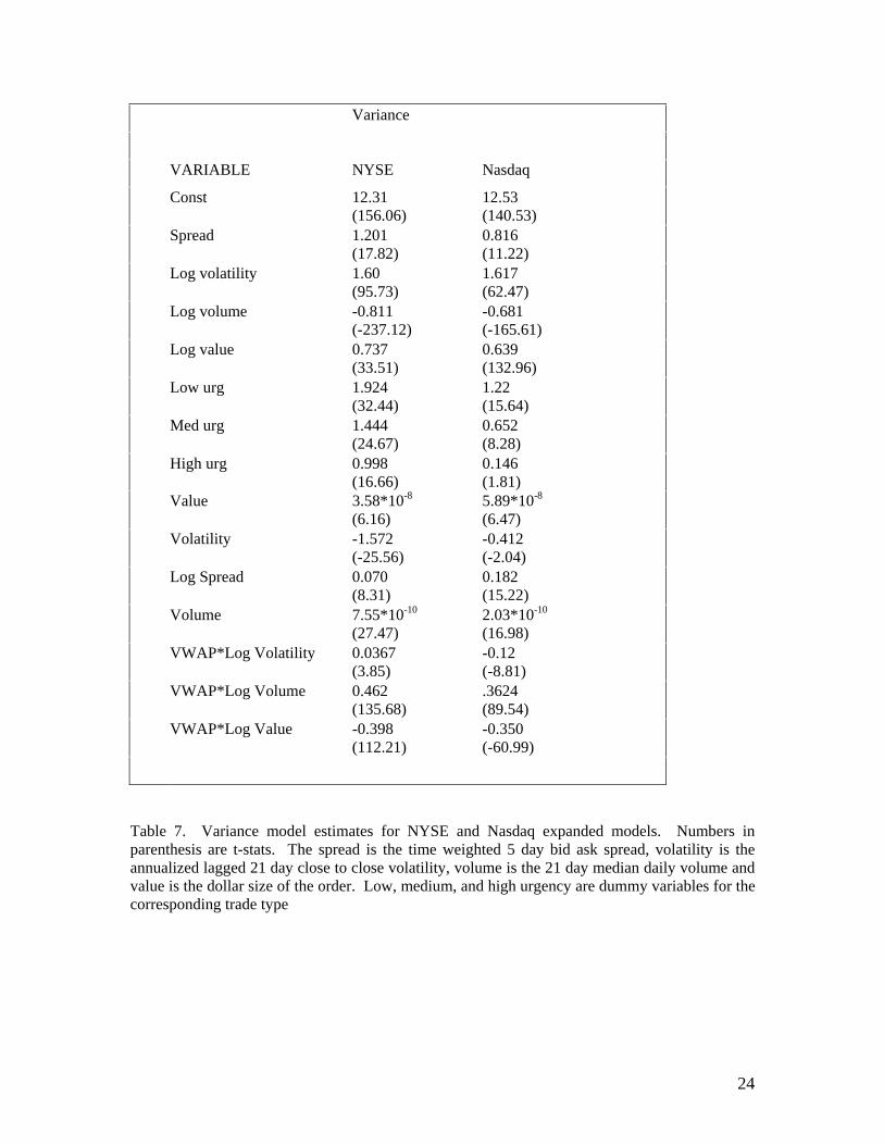
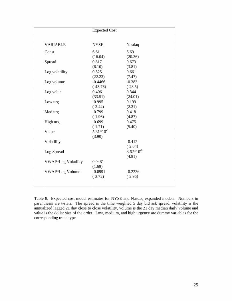
Tables 7 and 8 present the parameter estimates for the final, more detailed model that
passes the LM tests against the general alternative. The final model for the variance contains the
same variables for the NYSE orders and the Nasdaq orders although there are some differences in
the values of the coefficients. The models for the expected cost are different.
We begin our discussion with the variance models. The additional “nonlinear” terms are
the value, volatility, volume, (in levels) and the log spread. The elasticity of transaction risk with
respect to the size of the order is increasing in the order size. The volatility and volume variables
offset the logged terms so that larger volatility and volume result in elasticities that are smaller (in
absolute value).
There are three VWAP interaction terms with log volatility, log volume, and log value.
The signs on the log value and log volume are opposite the sign of the non-interacted
counterparts. This means that VWAP orders are less sensitive to the order size (as a fraction of
daily volume) than non VWAP orders. This makes sense since the VWAP orders do not directly
take risk into account but rather complete the trade over a specified time interval. The VWAP
16
term interacted with the log volatility is negative for the Nasdaq orders, but positive and
marginally significant for the NYSE orders. The volatility impact for both models is very small
relative to the non-interacted variable.
More pronounced differences between NYSE and Nasdaq occur in the models for the
expected cost. The log of the spread is needed in the expected cost equation for Nasdaq, but not
for NYSE. Nasdaq spreads are more informative than NYSE spreads regarding transaction costs
since most transactions in Nasdaq occur at the bid or the ask, unlike the NYSE where many
transaction prices occur strictly inside the spread. Perhaps it is not surprising then that the
Nasdaq model has a more complex dependence on the spread. The coefficient is positive on the
log spread variable indicating that expected costs should be more sensitive, and decrease more
quickly for the smallest spread stocks than found for NYSE stocks. The log volume term is
interacted with the VWAP. This suggests that VWAP trades are more sensitive to volume and
receive greater benefit than non-VWAP trades. Again, this could be due to the fact that VWAP
trades do not optimize with respect to trading costs or risk. The benefits of high volume are
therefore more important here to overcome the lack of optimization inherent in the strategy. The
other additional variables, while statistically significant are small in terms of economic impact.
VIII. Is the risk component economically meaningful?
In this section we examine the economic implications of the risk component. We ask two
questions. First, how important is the transaction risk component in the transaction decision?
Second, how what kind of risk aversion is consistent with traders execution choices?
In order to address these questions we consider a trader with expected utility given by
( ) ( ) ( )E U E TC V TCλ= − − . This is the standard mean variance utility but since TC denotes a
transaction cost and not a return we take the negative. We ask how much money would the trader
be willing to pay in order to transact risklessly. In this setting, ( )V TCλ represents the amount
of expected costs the trader would be willing to incur in order to transact risklessly. Similarly,
the risk adjusted transaction cost can be defined as
(7) ( )RATC TC V TCλ= −
Obviously this depends upon the choice of the risk aversion parameter λ . There is a large
literature that argues that this parameter may range from 0 to 15. See for example Friend and
Blume (1975) and Chou, Engle and Kane (1992) for empirical estimates. A reasonable value is 3
although this may suggest substantial risk tolerance. Considerably higher values should also be
17
considered. Figure 13 presents a plot of the cost of risk for NYSE and Nasdaq stocks for the four
different trade types. The VWAP trades have the highest cost of risk at about half a basis point
and the high urgency trades have the smallest cost of risk at about 1/20th of a basis point. A
typical trade has an expected cost of around 4 basis points. For higher urgency trades the cost of
risk is non-trivial. Furthermore, the small effects will be compounded when a portfolio is actively
managed.
We next examine what the choice of execution strategy implies about the traders risk
aversion. Since the frontier is piecewise linear, a range of values of λ will be consistent with a
given strategy yielding optimal utility. We solve for the range of values of λ for a typical trade
under normal conditions. We also consider large orders (10th percentile) and small orders (90th
percentile). The results are given in table 9. We find that VWAP is consistent with realistic
values of λ, typically smaller than 3. The low urgency trades are also often consistent with
reasonable risk aversion levels, but the medium and high urgency trades are not, generally
requiring exceptionally high risk aversion to be optimal. Interestingly, we find that traders often
use strategies that imply extreme risk aversion. The Nasdaq conditional frontier is not completely
convex so that medium urgency orders are not optimal for any value of λ.
IX. The Distribution of Transaction Cost and Liquidation Value at Risk (LVaR)
Liquidation risk is the uncertainty about how much it costs to liquidate a position in a timely
manner. Liquidation risk is important from both an asset management/risk perspective, as well as
a more recent literature on asset pricing and liquidity (see for example Easley and O’Hara (2003),
Pastor and Stambaugh (2003), Pedersen and Acharya (2005)). The conditional distribution of
transaction costs provides a detailed description of liquidation risk. For a given position,
liquidation execution strategy, and set of market conditions our model describes the probability
distribution of the cash value of the position after liquidating. One measure that summarizes the
liquidation risk is the liquidation value at risk or LVaR. Like the traditional value at risk (VaR),
LVaR tells us the minimum number of dollars that will be lost with some probability α, when
liquidating an asset.
For a given liquidation order the conditional mean and variance can be constructed. Under a
normality assumption, one can construct an α% LVAR given by:
(8) ( ) ( ) 11ˆ ˆexp exp2
LVaR X X z αα β γ −⎛ ⎞= + ⎜ ⎟⎝ ⎠

18
where α−1z is the 1-α % quantile.
More generally, we might not wish to impose the normality assumption and instead use a
semi-parametric approach. In the first stage, consistent estimates or the parameters can be
estimated by QMLE. In the second stage, the standardized residuals can be used to construct a
non-parametric estimate of the density function of the errors ε. The standardized residuals are
given by:
(9)
A non-parametric estimate of the density or perhaps just the quantiles themselves can then be
used to construct a semi-parametric LVaR. Specifically, let denote a non-parametric
estimate of the α% quantile of the density function of the error term ε. Then the semi-parametric
α% LVAR is obtained by replacing z1-α with the non-parametric quantile αε −1 :
(10) ( ) ( ) 1ˆ ˆ ˆexp exp2
LVaR X X αα β γ ε⎛ ⎞= + ⎜ ⎟⎝ ⎠
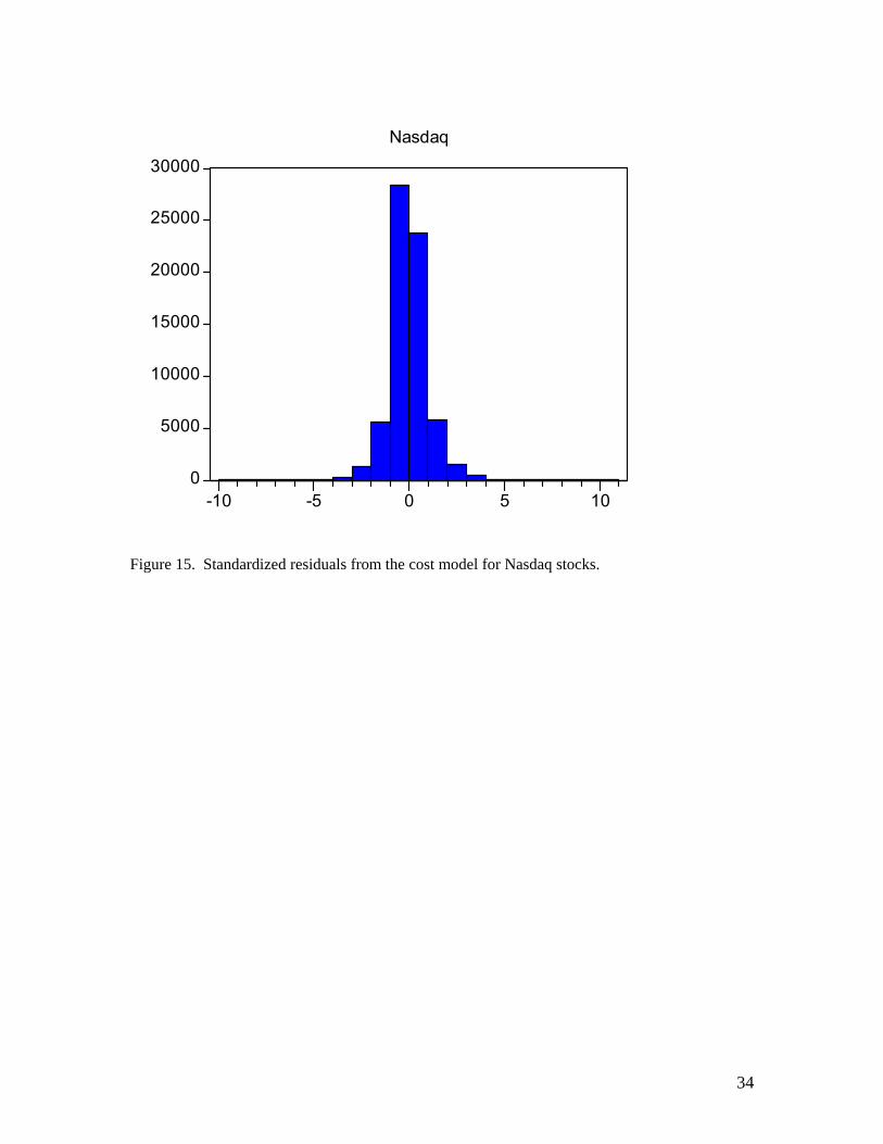
Figures 14 and 15 present the standardized residuals for the NYSE and Nasdaq models. The
residuals are clearly non-normal. We use the empirical quantiles of the data to construct the
LVaR. Figures 16 and 17 present the 1% LVaR associated with the high, medium and low
urgency orders as well as the VWAP. The LVaR estimates are constructed for typical stocks on a
typical day. The vertical axis is the transaction cost in basis points. As we move from left to
right we move from LVaR to low urgency to the high urgency orders. The LVaR is given by the
upper bar for each order type. The expected cost for each order type is given by the smaller bar
in near the origin. The differences in the mean are small relative to the changes in the risk across
the different order types. Since the risk dominates, the minimum LVaR order type here is given
by the most aggressive strategy, the high urgency order. The 1% LVaR for this order type is just
under around half a percent for NYSE and 1% for Nasdaq. For each order type the lower dashed
line completes a 98% prediction interval.
X. Conclusion
This paper demonstrates that expected cost and risk components of transaction costs can be
estimated from detailed transaction data. We show how to build mean variance frontiers for
different trading strategies. We find that the (conditional) expected cost and risk components can
( )⎟⎠⎞
⎜⎝⎛−
=γ
βεˆ
21exp
ˆexp%ˆ
i
iii
X
XTC
αε −1

19
be modeled using an exponential specification for the mean and variance. Characteristics of the
order and state of the market play an important role in determining the cost/risk tradeoff faced by
the trader.
After controlling for order and market characteristics we show that for moderate utility
functions the value of the risk is considerably smaller than the value of the mean of transaction
cost, but is non-negligible and can compound when portfolios are actively managed. In an
important step forward in the analysis of execution costs, we show how to risk adjust execution
costs and find that the traders often appear very risk averse when choosing an execution strategy.
Our model for the conditional distribution of transaction costs completely describes
liquidation risk. We provide an example of how this conditional distribution can be used to
assess portfolio liquidation risk using the notion of liquidation value at risk (LVAR). There are,
of course, many other possible measures of liquidation risk that could be constructed using the
conditional distribution.
This general approach can be used to compare various execution technologies, exchanges
and liquidity search engines and it should prove a useful tool for clients to compare the
performance of alternative brokers or algorithmic traders. Unlike existing measures, the proposed
approach accounts for both average cost and, importantly, risk. When embedded in a portfolio
model it allows stock selection with better control of execution costs.

20
Table 1. Summary statistics for Morgan Stanley trades sorted by Exchange (NYSE and Nasdaq), side of trade where B and S are buy and sell orders respectively, the transaction type where A and V are arrival price and VWAP strategies and H, M, and L correspond to high, medium and low urgency trades. Weight denotes the sample fraction of order volume and count is the actual number of orders. Spread denotes the 5-day time weighted bid-ask spread. Volatility is the annualized 21 day volatility. Volume is the size of the order expressed as a fraction of the 21 day median volume. Order value is the dollar size of the order and order shares is the number of shares. Cost is the average transaction cost (TC) expressed in basis points and StDev is the standard deviation of the transaction cost.
Exchange Side Benchmark Urgency Weight Count Price Spread Volatility VolumeCapitalization
(000)Order Value
Order Shares
Cost (BP)
StDev (BP)
100% 233,913 45.07$ 0.09% 26% 1.59% 59,609,060$ 310,472$ 9,154 10.09 47.24B 62% 147,649 45.06$ 0.09% 26% 1.57% 58,137,900$ 302,812$ 8,946 10.77 47.17S 38% 86,264 45.09$ 0.08% 26% 1.62% 61,965,453$ 323,583$ 9,512 8.99 47.31
NYSE 75% 166,508 48.01$ 0.09% 23% 1.68% 66,717,110$ 326,031$ 8,701 8.82 43.28NASDAQ 25% 67,405 36.38$ 0.08% 36% 1.33% 38,565,201$ 272,037$ 10,273 13.84 57.19
A H 10% 15,616 47.81$ 0.08% 26% 1.18% 60,838,460$ 475,462$ 12,845 11.69 23.19A M 24% 54,095 44.73$ 0.09% 27% 1.47% 48,482,781$ 320,909$ 9,688 11.09 32.20A L 20% 51,588 46.44$ 0.08% 26% 1.13% 68,894,693$ 285,018$ 8,106 8.99 40.89V 46% 112,614 44.04$ 0.09% 26% 1.95% 61,042,206$ 294,240$ 8,867 9.69 59.01

21
Table 2. Summary statistics for Morgan Stanley trades sorted by Exchange (NYSE and Nasdaq), side of trade where B and S are buy and sell orders respectively, the transaction type where A and V are arrival price and VWAP strategies and H, M, and L correspond to high, medium and low urgency trades. Weight denotes the sample fraction of order volume and count is the actual number of orders. Spread denotes the 5-day time weighted bid-ask spread. Volatility is the annualized 21 day volatility. Volume is the size of the order expressed as a fraction of the 21 day median volume. Order value is the dollar size of the order and order shares is the number of shares. Cost is the average transaction cost (TC) expressed in basis points and StDev is the standard deviation of the transaction cost.
Exchange Benchmark UrgencyVolume Range Weight Count Price Spread Volatility Volume
Capitalization (000) Order Value
Cost (BP)
StDev (BP)
NYSE A H ≤ 0.25% 0.69% 2,630 47.77$ 0.08% 22% 0.19% 94,061,545$ 190,107$ 4.22 10.97NYSE A M 3.10% 13,664 48.06$ 0.08% 22% 0.16% 95,714,257$ 164,767$ 3.69 11.64NYSE A L 4.17% 19,379 50.15$ 0.08% 22% 0.14% 98,487,506$ 156,371$ 2.71 12.74NYSE V 6.54% 38,116 47.46$ 0.08% 22% 0.13% 90,733,082$ 124,606$ 1.97 34.56NYSE A H ≤ 0.5% 1.69% 3,559 51.00$ 0.08% 22% 0.37% 81,476,811$ 345,605$ 6.16 11.95NYSE A M 3.30% 9,557 49.09$ 0.08% 23% 0.36% 68,991,562$ 250,562$ 5.68 15.53NYSE A L 2.99% 8,027 50.18$ 0.08% 21% 0.36% 92,105,328$ 270,537$ 4.15 19.65NYSE V 5.00% 14,890 48.23$ 0.08% 23% 0.37% 65,205,449$ 244,088$ 3.06 42.27NYSE A H ≤ 1.0% 2.39% 2,979 52.69$ 0.08% 22% 0.73% 72,154,182$ 582,738$ 8.93 15.98NYSE A M 3.64% 6,907 48.85$ 0.08% 24% 0.72% 54,822,342$ 383,195$ 7.54 20.67NYSE A L 3.17% 6,035 50.22$ 0.08% 22% 0.72% 82,177,737$ 381,487$ 6.76 28.64NYSE V 6.40% 11,822 46.88$ 0.09% 23% 0.73% 71,181,217$ 393,015$ 5.17 47.42NYSE A H > 1.0% 2.67% 2,549 51.53$ 0.09% 23% 2.31% 48,375,509$ 760,186$ 14.36 25.12NYSE A M 7.34% 7,052 47.41$ 0.10% 24% 3.02% 36,941,147$ 755,825$ 15.55 38.97NYSE A L 4.77% 5,632 47.78$ 0.10% 23% 2.55% 52,146,046$ 615,387$ 12.64 52.73NYSE V 16.88% 13,710 45.67$ 0.09% 23% 3.95% 54,313,103$ 894,247$ 14.66 65.61NASDAQ A H ≤ 0.25% 0.28% 715 36.70$ 0.06% 33% 0.18% 76,072,230$ 288,664$ 6.58 12.91NASDAQ A M 1.59% 5,771 37.81$ 0.06% 34% 0.15% 52,884,846$ 200,367$ 6.05 17.13NASDAQ A L 1.36% 5,065 37.49$ 0.06% 33% 0.14% 77,185,322$ 195,338$ 5.29 17.93NASDAQ V 3.73% 16,227 39.02$ 0.06% 34% 0.11% 71,786,694$ 167,134$ 3.96 42.05NASDAQ A H ≤ 0.5% 0.82% 1,131 39.07$ 0.06% 32% 0.37% 63,042,552$ 527,242$ 10.76 18.02NASDAQ A M 1.35% 4,455 36.72$ 0.08% 36% 0.36% 30,091,409$ 220,816$ 9.15 21.53NASDAQ A L 0.89% 2,578 38.02$ 0.07% 36% 0.37% 37,310,972$ 251,330$ 8.33 31.04NASDAQ V 1.64% 5,597 35.82$ 0.07% 36% 0.36% 45,881,902$ 213,288$ 6.07 59.83NASDAQ A H ≤ 1.0% 0.85% 992 38.30$ 0.07% 35% 0.70% 42,108,883$ 623,028$ 15.81 21.17NASDAQ A M 1.31% 3,453 36.58$ 0.09% 38% 0.71% 15,709,279$ 275,812$ 14.78 30.01NASDAQ A L 0.97% 2,003 39.11$ 0.07% 37% 0.72% 32,386,856$ 352,916$ 12.36 45.50NASDAQ V 1.80% 5,310 34.08$ 0.08% 36% 0.73% 36,671,191$ 246,208$ 10.62 66.66NASDAQ A H > 1.0% 0.83% 1,061 37.41$ 0.10% 36% 2.91% 10,249,188$ 565,871$ 26.99 47.16NASDAQ A M 2.26% 3,236 32.85$ 0.11% 39% 3.10% 8,045,030$ 508,137$ 22.96 58.51NASDAQ A L 1.91% 2,869 36.91$ 0.10% 38% 2.85% 15,236,379$ 484,223$ 26.02 79.01NASDAQ V 3.62% 6,942 33.30$ 0.11% 37% 3.46% 23,073,584$ 379,150$ 24.65 94.67

22
VARIABLE COEFFICIENT ROBUST T-STAT
Const 11.80559 90.86393
Spread 1.815802 14.39896
Log volatility 1.207152 64.98954
Log volume -0.51614 -55.6044
Log value 0.536306 46.08766
Low urg -1.45436 -83.2275
Med urg -1.92541 -61.058
High urg -2.33731 -88.2665
Table 3. Variance parameter estimates for NYSE stocks. The spread is the time weighted 5 day bid ask spread, volatility is the annualized lagged 21 day close to close volatility, volume is the 21 day median daily volume and value is the dollar size of the order. Low, medium, and high urgency are dummy variables for the corresponding trade type.
VARIABLE COEFFICIENT ROBUST T-STAT
Const 5.173827 30.0342
Spread 0.969804 8.395586
Log volatility 0.503987 21.14475
Log volume -0.47084 -43.4163
Log value 0.43783 40.27979
Low urg 0.094929 2.41284
Med urg 0.305623 8.796438
High urg 0.41034 11.28093
Table 4. Mean parameter estimates for NYSE stocks. The spread is the time weighted 5 day bid ask spread, volatility is the annualized lagged 21 day close to close volatility, volume is the 21 day median daily volume and value is the dollar size of the order. Low, medium, and high urgency are dummy variables for the corresponding trade type.

23
VARIABLE COEFFICIENT ROBUST T-STAT
Const 11.40519 71.44173 Spread 2.016026 17.00666 Log volatility 1.078963 40.27656 Log volume -0.44182 -46.7497 Log value 0.453704 42.64865 Low urg -1.04398 -42.1013 Med urg -1.70511 -65.0131 High urg -2.10623 -48.7398 Table 5. Variance parameter estimates for Nasdaq stocks. The spread is the time weighted 5 day bid ask spread, volatility is the annualized lagged 21 day close to close volatility, volume is the 21 day median daily volume and value is the dollar size of the order. Low, medium, and high urgency are dummy variables for the corresponding trade type.
VARIABLE COEFFICIENT ROBUST T-STAT
Const 5.354067 26.04098 Spread 1.014023 8.734035 Log volatility 0.513628 16.96502 Log volume -0.41447 -29.9304 Log value 0.376208 24.99588 Low urg 0.025356 0.243943 Med urg 0.230764 5.716912 High urg 0.282479 6.156517 Table 6. Mean parameter estimates for Nasdaq stocks. The spread is the time weighted 5 day bid ask spread, volatility is the annualized lagged 21 day close to close volatility, volume is the 21 day median daily volume and value is the dollar size of the order. Low, medium, and high urgency are dummy variables for the corresponding trade type.
24
Variance
VARIABLE NYSE Nasdaq
Const 12.31 (156.06)
12.53 (140.53)
Spread 1.201 (17.82)
0.816 (11.22)
Log volatility 1.60 (95.73)
1.617 (62.47)
Log volume -0.811 (-237.12)
-0.681 (-165.61)
Log value 0.737 (33.51)
0.639 (132.96)
Low urg 1.924 (32.44)
1.22 (15.64)
Med urg 1.444 (24.67)
0.652 (8.28)
High urg 0.998 (16.66)
0.146 (1.81)
Value 3.58*10-8
(6.16) 5.89*10-8 (6.47)
Volatility -1.572 (-25.56)
-0.412 (-2.04)
Log Spread 0.070 (8.31)
0.182(15.22)
Volume 7.55*10-10 (27.47)
2.03*10-10 (16.98)
VWAP*Log Volatility 0.0367 (3.85)
-0.12 (-8.81)
VWAP*Log Volume 0.462 (135.68)
.3624 (89.54)
VWAP*Log Value -0.398 (112.21)
-0.350 (-60.99)
Table 7. Variance model estimates for NYSE and Nasdaq expanded models. Numbers in parenthesis are t-stats. The spread is the time weighted 5 day bid ask spread, volatility is the annualized lagged 21 day close to close volatility, volume is the 21 day median daily volume and value is the dollar size of the order. Low, medium, and high urgency are dummy variables for the corresponding trade type
25
Expected Cost
VARIABLE NYSE Nasdaq
Const 6.61 (16.04)
5.69 (20.36)
Spread 0.817 (6.10)
0.673 (3.81)
Log volatility 0.525 (22.23)
0.661 (7.47)
Log volume -0.4466 (-43.76)
-0.383 (-28.5)
Log value 0.406 (33.51)
0.344 (24.01)
Low urg -0.995 (-2.44)
0.199 (2.21)
Med urg -0.799 (-1.96)
0.418 (4.87)
High urg -0.699 (-1.71)
0.475 (5.40)
Value 5.31*10-8
(3.90) Volatility
-0.412 (-2.04)
Log Spread
8.62*10-8
(4.81) VWAP*Log Volatility 0.0481
(1.69) VWAP*Log Volume -0.0991
(-3.72) -0.2236 (-2.96)
Table 8. Expected cost model estimates for NYSE and Nasdaq expanded models. Numbers in parenthesis are t-stats. The spread is the time weighted 5 day bid ask spread, volatility is the annualized lagged 21 day close to close volatility, volume is the 21 day median daily volume and value is the dollar size of the order. Low, medium, and high urgency are dummy variables for the corresponding trade type.

26
TYPICAL 10th Percentile Value 90th Percentile Value NYSE Nasdaq NYSE Nasdaq NYSE Nasdaq VWAP 0-3.7 0-1.5 0-3.0 0-1.1 0-5.8 0-2.4 Low 3.7-65.8 1.5-54.4 3.0-98.2 1.1-83.2 5.8-41.4 2.4-33.8 Med 65.8-71.1 98.2-106.3 41.4-44.8 High >71.1 >54.4 >106.3 >83.2 >44.8 >33.8 Table 9. This table presents the risk aversion values that are consistent with a given trading strategy optimizing the quadratic utility under average conditions for average volume (left) 10th percentile Value, or large trades, (middle) and 90th percentile, or small trades, (right).
27
Figure 1: NYSE average cost/risk tradeoff for different order sizes (<.25%, .25-.5%, .5-1%, and >1%). The order size is expressed as a fraction of the median 21 day daily volume. Each contour has four points - high urgency, medium urgency, low urgency, and VWAP (moving from left to right). Figure 2: Nasdaq average cost/risk tradeoff for different order sizes (<.25%, .25-.5%, .5-1%, and >1%). The order size is expressed as a fraction of the median 21 day daily volume. Each contour has four points - high urgency, medium urgency, low urgency, and VWAP (moving from left to right).
1.90
3.90
5.90
7.90
9.90
11.90
13.90
10.90 20.90 30.90 40.90 50.90 60.90
Stdev (BP)
Mea
n (B
P)
0.0025 0.0050 0.0100 > 0.0100
3.90
8.90
13.90
18.90
23.90
12.90 22.90 32.90 42.90 52.90 62.90 72.90 82.90 92.90
Stdev (BP)
Mea
n (B
P)
0.0025 0.0050 0.0100 > 0.0100
28
0
5
10
15
20
25
30
0 0.5 1 1.5 2
Bas
is P
oint
s
Value/Volume
NYSE Expected Cost
VWAP
low
med
high
Figure 3: Expected cost as a function of the order size expressed as a fraction of average daily volume for an NYSE stock under “normal” conditions.
0
20
40
60
80
100
120
0 0.5 1 1.5 2
Bas
is P
oint
s
Value/Volume
NYSE Standard Deviation
VWAP
low
med
high
Figure 4: Standard deviation of transaction cost as a function of the order size expressed as a fraction of average daily volume for an NYSE stock under “normal” conditions.
29
0
5
10
15
20
25
30
35
40
0 0.5 1 1.5 2
Bas
is P
oint
s
Value/Volume
Nasdaq Expected Cost
VWAP
low
med
high
Figure 5. Expected Cost as a function of the order size expressed as a fraction of average daily volume for a Nasdaq stock under “normal” conditions.
0
20
40
60
80
100
120
140
0 0.5 1 1.5 2
Bas
is P
oint
s
Value/Volume
Nasdaq Standard Deviation
VWAP
low
med
high
Figure 6. Standard deviation of transaction cost as a function of the order size expressed as a fraction of average daily volume for a Nasdaq stock under “normal” conditions.

30
0
1
2
3
4
5
6
7
8
9
0 10 20 30 40 50
Volatility
NYSE
Exp
ecte
d C
ost
Figure 7. Expected cost and risk frontier for a typical NYSE stock on a typical day. Ellipses denote 95% confidence intervals around high urgency, medium urgency, low urgency, and VWAP order types (from left to right) under “normal” conditions.
0
1
2
3
4
5
6
7
8
9
0 10 20 30 40 50
NASDAQ
Volatiltiy
Exp
ecte
d C
ost
Figure 8. Expected cost and risk frontier for a typical Nasdaq stock on a typical day. Ellipses denote 95% confidence intervals around high urgency, medium urgency, low urgency, and VWAP order types (from left to right) under “normal” conditions.

31
0
2
4
6
8
10
12
14
0 10 20 30 40 50 60 70
10th25th50th
75th90th
NYSE Frontier by Order Size Percentile
Volatility
Exp
ecte
d C
ost
Figure 9. Expected cost/risk frontier for a typical NYSE stock on a typical day. Each contour has four points corresponding to high urgency, medium urgency, low urgency, and VWAP orders (from left to right) representing the frontier for different quantiles of order size expressed as a fraction of average daily volume.
0
4
8
12
16
20
0 10 20 30 40 50 60 70 80 90
10th 25th 50th
75th 90th
NASDAQ Frontier by Order Size Percentile
Volatility
Exp
ecte
d C
ost
Figure 10. Expected cost/risk frontier for a typical Nasdaq stock on a typical day. Each contour has four points corresponding to high urgency, medium urgency, low urgency, and VWAP orders (from left to right) representing the frontier for different quantiles of order size expressed as a fraction of average daily volume.

32
Figure 11. Nasdaq and NYSE mean variance transaction cost frontiers for identical trades under identical conditions. Each contour has four points corresponding to high urgency, medium urgency, low urgency, and VWAP orders (from left to right).
Figure 12. Nasdaq and NYSE mean variance transaction cost frontiers for identical trades under identical conditions assuming that Nasdaq volume is 30% overstated. Each contour has four points corresponding to high urgency, medium urgency, low urgency, and VWAP orders (from left to right).

33
0
0.05
0.1
0.15
0.2
0.25
0.3
0.35
0.4
0.45
0.5
VWAP Low Medium High
NYSE NASDAQ
Figure 13. The cost of risk for the VWAP, Low, Medium, and High urgency orders for a quadratic utility investor with risk aversion parameter of 3 for NYSE and Nasdaq stocks.
0
10000
20000
30000
40000
50000
60000
70000
80000
-10 -5 0 5 10 15 20 25
NYSE
Figure 14. Standardized residuals from the cost model for NYSE stocks.
34
0
5000
10000
15000
20000
25000
30000
-10 -5 0 5 10
Nasdaq
Figure 15. Standardized residuals from the cost model for Nasdaq stocks.

35
\Figure 16. This plot shows the 98% predictive interval for the transaction cost for a typical NYSE stock on a typical day. 0 corresponds to VWAP, 1 to low urgency, 2 to medium urgency and 3 to high urgency. For each trade type, the upper bar denotes the 1% LVAR. Figure 17. This plot shows the 98% predictive interval for the transaction cost for a typical Nasdaq stock on a typical day. 0 corresponds to VWAP, 1 to low urgency, 2 to medium urgency and 3 to high urgency. For each trade type, the upper bar denotes the 1% LVAR.
98% Predictive Interval for Typical Conditions (NASDAQ)
-200-150-100
-500
50100150200250
0 1 2 3 4
Tran
sact
ion
Cos
t
98% Predictive Interval for Typical Conditions (NYSE)
-150
-100
-50
0
50
100
150
0 1 2 3 4
Tran
sact
ion
Cos
t
RN-VWAP Low Urgency
High Urgency
Med Urgency
RN-VWAP Med Urgency
High Urgency
Low Urgency

36
References Acharya, Viral and Lasse Pederson(2005), “Asset Pricing with Liquidity Risk” Journal of
Financial Economics,vol 11, pp.375-410 Almgren, Robert and Neil Chriss, (1999) “Value under Liquidation”, Risk, 12 Almgren, Robert and Neil Chriss,(2000) “Optimal Execution of Portfolio Transactions,” Journal
of Risk, 3, pp 5-39 Almgren, Robert,(2003) “Optimal Execution with Nonlinear Impact Functions and Trading-
enhanced Risk”, Applied Mathematical Finance, 10,pp1-18 Bertsimas, Dimitris, and Andrew W. Lo, (1998) “Optimal Control of Execution Costs,” Journal
of Financial Markets, 1, pp1-50 Bessembinder, Hendrik, (2003) “Issues in Assessing Trade Execution Costs”, Journal of
Financial Markets, Vol 6, pp 233-257 Chan, Louis K. and Josef Lakonishok, (1995) “The Behavior of Stock Prices around Institutional
Trades”, Journal of Finance, Vol 50, No. 4, pp1147-1174 Chou, Ray, Robert Engle and Alex Kane,(1992)”Measuring risk aversion from excess returns on
a stock index”, Journal of Econometrics, 52, pp201-224 Easley, David, Soeren Hvidkjaer, and Maureen O’Hara, 2002, Is information risk a determinant
of asset returns? Journal of Finance 57, 2185-2222. Engle, Robert, and Robert Ferstenberg, 2007, Execution Risk, Journal of Portfolio Management,
V33, I2, pp 34-45 Friend, Irwin and Marshall Blume,(1975) “The Demand for Risky Assets”, American Economic
Review, Vol65, pp 900-922 Grinold R. and R. Kahn(1999) Active Portfolio Management (2nd Edition) Chapter 16 pp473-475,
McGraw-Hill Lehmann, Bruce,(2003) “What We Measure in Execution Cost Measurement”, Journal of
Financial Markets, Vol 6, pp 227-231 Obizhaeva, Anna and Jiang Wang (2005) “Optimal Trading Strategy and Supply/Demand
Dynamics” manuscript Pastor, Lubos, Robert Stambaugh, (2003), “Liquidity Risk and Expected Stock Returns”, Journal
of Political Economy 111, 642–685. Peterson, Mark and Eric Sirri, (2003) “Evaluation of the Biases in Execution Cost Estimation
Using Trade and Quote Data”, Journal of Financial Markets, Vol 6, pp 259-280
37
Werner, Ingrid, (2003) “NYSE Order Flow, Spreads and Information”, Journal of Financial
Markets, Vol 6, pp 309-335 White, Halbert, 1982, Maximum Likelihood Estimation of Misspecified Models, Econometrica,
50, 1-25.