measuring the efficiency of the turkish electric distribution sector

MEASURING THE EFFICIENCY OF THE TURKISH ELECTRIC DISTRIBUTION SECTOR USING STOCHASTIC FRONTIER ANALYSIS

A THESIS SUBMITTED TO GRADUATE SCHOOL OF NATURAL AND APPLIED SCIENCES

OF MIDDLE EAST TECHNICAL UNIVERSITY

BY

AYDIN ÇELEN

IN PARTIAL FULFILLMENT OF THE REQIREMENTS FOR

THE DEGREE OF MASTER OF SCIENCE IN

INDUSTRIAL ENGINEERING

FEBRUARY 2011

ii

Approval of the thesis:


submitted by AYDIN ÇELEN in partial fulfillment of the requirements for the degree of Master of Science in Industrial Engineering Department, Middle East Technical University by, Prof. Dr. Canan ÖZGEN Dean, Graduate School of Natural and Applied Sciences ____________________ Prof. Dr. Sinan KAYALIGİL Head of Department, Industrial Engineering __________________ Assist. Prof. Dr. Cem İYİGÜN Supervisor, Industrial Engineering Dept., METU __________________ Examining Committee Members: Prof. Dr. Meral AZİZOĞLU Industrial Engineering Dept., METU __________________ Assist. Prof. Dr. Cem İYİGÜN Industrial Engineering Dept., METU __________________ Assoc. Prof. Dr. Uğur SOYTAŞ Business Administration Dept., METU __________________ Assist. Prof. Dr. Serhan DURAN Industrial Engineering Dept., METU __________________ Assist. Prof. Dr. Z.Pelin BAYINDIR Industrial Engineering Dept., METU __________________

Date: February 10, 2011

iii

I hereby declare that all information in this document has been obtained and presented in accordance with academic rules and ethical conduct. I also declare that, as required by these rules and conduct, I have fully cited and referenced all material and results that are not original to this work. Name, Last name : Aydın ÇELEN

Signature :

iv

ABSTRACT


ÇELEN, Aydın

M.Sc., Department of Industrial Engineering

Supervisor: Assist. Prof. Dr. Cem İYİGÜN

February 2011, 117 pages

This study analyzes the technical efficiencies of Turkish electricity distribution

companies (21 in total) throughout 2002 and 2009. For this aim, we used six

different model specifications, all of which are generated from two different

Stochastic Frontier Analysis (SFA) models (Battese ve Coelli (1992&1995)).

At the end of the estimations of the models, it has been seen that the signs and

significance levels of the coefficient estimations are very consistent and satisfactory

in all models. We also observed consistency between the coefficient estimations of

the different models despite the differences in the magnitudes of the coefficient

estimations. For example, all model specifications confirm the presence of increasing

returns to scale and of a mild technological progress over time in the market. In

addition, among the inputs, all inputs except the quality of the electricity delivered

are important in enhancing technical efficiency of the electricity distribution

companies, according to the all alternative specifications. Again, all models showed

that inefficiency effects rather than random error effects are of crucial importance in

Turkish electricity distribution market.

As for the efficiency estimations of the alternative models, the main conclusion

revealed by our study is that efficiency estimations of the Battese ve Coelli (1995)

v

models are remarkably higher than those of the Battese ve Coelli (1992) models. The

efficiency estimation differences between Battese and Coelli (1992&1995) models

can be attributed to the environmental variables included into the Battese ve Coelli

(1995) models, which are not generally controlled by electricity distribution

companies.

Keywords: Technical Efficiency, Turkish Electricity Distribution Market, Stochastic

Frontier Analysis (SFA).

vi

ÖZ

TÜRKİYE ELEKTRİK DAĞITIM SEKTÖRÜNÜN ETKİNLİĞİNİN STOKASTİK SINIR ANALİZİ KULLANILARAK ÖLÇÜLMESİ

ÇELEN, Aydın

Yüksek Lisans, Endüstri Mühendisliği Bölümü

Tez Yöneticisi: Yrd. Doç. Dr. Cem İYİGÜN

Şubat 2011, 117 sayfa

Bu çalışma, 2002 ve 2009 yılları arasında Türkiye elektrik dağıtım şirketlerinin

(toplam 21) teknik etkinliklerini analiz etmektedir. Bu amaçla, tamamı iki farklı

Stokastik Sınır Analizi (SFA) modelinden (Battese ve Coelli (1992&1995))

türetilmiş altı farklı model tanımlaması kullandık.

Modellerin tahmini neticesinde, katsayı tahminlerinin işaret ve anlamlılık

düzeylerinin çok tutarlı ve tatmin edici olduğu görülmüştür. Katsayı tahminlerinin

büyüklüklerinde farklılıklar olmasına rağmen, farklı modellerin katsayı tahminleri

arasında da tutarlılıklar gözlemledik. Örneğin, tüm modeller, pazarda ölçeğe göre

artan getiri ve zamanla yavaş bir teknolojik ilerlemenin varlığını onaylamaktadır.

Ayrıca, tüm alternatif modellere göre, girdiler içerisinde, dağıtılan elektriğin kalitesi

hariç tüm girdiler elektrik dağıtım şirketlerinin teknik etkinliklerinin

iyileştirilmesinde önemlidir. Yine tüm modeller, Türkiye elektrik dağıtım pazarında

rassal hata etkisinden ziyade etkinsizlik etkisinin kritik öneme sahip olduğunu

göstermiştir.

Alternatif modellerin etkinlik tahminlerine gelince, bu çalışmadan çıkan ana sonuç,

Battese ve Coelli (1995) modellerinin etkinlik tahminlerinin Battese ve Coelli (1992)

vii

modellerinin etkinlik tahminlerinden önemli ölçüde yüksek olduğudur. Battese ve

Coelli (1992&1995) modellerinin etkinlik tahminleri arasındaki farklılıklar, Battese

ve Coelli (1995) modellerine dahil edilmiş olan, genellikle elektrik dağıtım şirketleri

tarafından kontrol edilemeyen çevresel değişkenlere bağlanabilir.

Anahtar Kelimeler: Teknik Etkinlik, Turkiye Elektrik Dağıtım Pazarı, Stokastik

Sınır Analizi (SFA).

viii

To my wife Alev and my son Murat Kaan

ix

ACKNOWLEDGEMENTS

I would like to express my thanks to Assist. Prof. Dr. Cem İYİGÜN for his

wonderful supervision. Studying with him was a great experience for me. I also

express my deepest gratitude to other examining committee members, Prof. Dr.

Meral AZİZOĞLU, Assoc. Prof. Dr. Uğur SOYTAŞ, Assist. Prof. Dr. Serhan

DURAN and Assist. Prof. Dr. Z.Pelin BAYINDIR, for their valuable contributions

and comments.

I would like to thank my father and mother. I always feel their unlimited support and

belief to me throughout my life. I would also like to express my appreciation to my

parents-in-law for their supports and understandings.

My special thanks are due to two people, my wife Alev and my son Murat Kaan for

being in my life, and for making me feel that I am the luckiest person in the world.

.

x

TABLE OF CONTENTS

ABSTRACT ........................................................................................................... iv ÖZ ......................................................................................................................... vi ACKNOWLEDGEMENTS..................................................................................... ix TABLE OF CONTENTS ..........................................................................................x LIST OF TABLES ................................................................................................. xii LIST OF FIGURES................................................................................................xiv LIST OF ABBREVIATIONS..................................................................................xv CHAPTERS 1. INTRODUCTION ............................................................................................. 1 2. TURKISH ELECTRICITY MARKET............................................................... 5

2.1. GENERAL CHARACTERISTICS OF ELECTRICITY AND ELECTRICITY MARKETS......................................................................... 5

2.2. HISTORICAL EVALUATION OF TURKISH ELECTRICITY MARKET. 7 2.2.1. Pre-TEK period (1913-1970) .............................................................. 7 2.2.2. TEK period (1970-1993)..................................................................... 9 2.2.3. Post-TEK period (1994-ongoing) .......................................................10

2.3. CURRENT STRUCTURE OF TURKISH ELECTRICITY MARKET .......19 3. METHODOLOGY AND LITERATURE SURVEY .........................................36

3.1. DEFINITIONS...........................................................................................36 3.1.1. Efficiency ..........................................................................................36 3.1.2. Technology Set ..................................................................................39 3.1.3. Output Set..........................................................................................40 3.1.4. Production Possibility Curve (Output Isoquant) .................................41 3.1.5. Input Set ............................................................................................42 3.1.6. Input Isoquant ....................................................................................43 3.1.7. Distance Functions.............................................................................44 3.1.7.1. Output Distance Functions ..............................................................44 3.1.7.2. Input Distance Functions.................................................................46 3.1.8. Technical Efficiency ..........................................................................47 3.1.8.1. Output-Oriented Technical Efficiency.............................................48 3.1.8.2. Input-Oriented Technical Efficiency ...............................................49

3.2. EFFICIENCY MEASUREMENT...............................................................50 3.2.1. Data Envelopment Analysis (DEA)....................................................51 3.2.2. Stochastic Frontier Analysis (SFA) ....................................................55 3.2.3. Comparison of DEA and SFA............................................................61

xi

4. MODELS AND DATA.....................................................................................63 4.1. MODELS ...................................................................................................63

4.1.1. Battese and Coelli (1992)...................................................................67 4.1.2. Battese and Coelli (1995) ...................................................................68

4.2. MODEL SPECIFICATIONS AND DATA.................................................70 5. ESTIMATION RESULTS ................................................................................78

5.1. ESTIMATION RESULTS FOR ALTERNATIVE BC92 MODELS ...........78 5.2. ESTIMATION RESULTS FOR ALTERNATIVE BC95 MODELS ...........86 5.3. COMPARISON BETWEEN ALTERNATIVE BC92&BC95 MODELS ....95

6. CONCLUSION & FURTHER STUDIES .........................................................98 REFERENCES .....................................................................................................105 APPENDIX A.......................................................................................................110

GRAPHS OF VARIABLES ............................................................................110

xii

LIST OF TABLES

TABLES

Table 2.1. Electricity Distribution Companies and Regions ...................................13

Table 2.2. Current Situation in Privatization of Electricity Distributions................17

Table 2.3. Installed Capacity and Generation in Turkey ........................................20

Table 2.4. Annual Development of Turkey's Electricity Generation By Primary Energy Resources .................................................................................21

Table 2.5. Electricity Generation, Imports, Exports and Gross Supply of OECD Countries in 2009 (Estimate) ................................................................23

Table 2.6. Installed Capacity of OECD Countries in 2008.....................................24

Table 2.6. (cont’d) Installed Capacity of OECD Countries in 2008........................25

Table 2.7. Annual Development of Turkey's Electricity Generation By the Electric Utilities.................................................................................................27

Table 2.8. The Distribution of Gross Electricity Generation by Primary Energy Resources and the Electricity Utilities in 2009 ......................................29

Table 2.9. Annual Development of Electricity Generation, Consumption, Imports, Exports and Consumption.....................................................................30

Table 2.10. Per Capita Electricity Capacity, Generation and Consumption in Turkey.............................................................................................................32

Table 2.11. Per Capita Electricity Capacity, Generation and Supply of OECD Countries in 2008 .................................................................................33

Table 2.12. Electricity Prices of Some OECD Countries According to OECD Mean in 2008 .................................................................................................34

Table 2.13. Cost Structure of Electricity Price Paid by a Household in Turkey in 2008 .....................................................................................................35

Table 4.1. Specification of Models ........................................................................72

Table 4.2. Descriptive Statistics ............................................................................75

Table 4.3. Descriptive Statistics_Mean values over the period 1992-1999.............76

Table 5.1. Estimation Results of Alternative BC92 Models ...................................79

xiii

Table 5.2. Technical Efficiency Scores for Model BC92-1 ....................................82



Table 5.5. Average Efficiency Scores for Alternative BC92 Models......................85

Table 5.6. Summary Statistics of Technical Efficiency Scores for Alternative BC92 Models .................................................................................................86

Table 5.7. Estimation Results of Alternative BC95 Models ...................................87




Table 5.11. Average Efficiency Scores for Alternative BC95 Models......................94

Table 5.12. Summary Statistics of Technical Efficiency Scores for Alternative BC95 Models .................................................................................................94

Table 5.13. Correlations of Technical Efficiency Scores Using Alternative Models.97

Table 5.14. Correlations of Rankings Using Alternative Models .............................97

xiv

LIST OF FIGURES

FIGURES

Figure 2.1. Electricity Distribution Regions............................................................14

Figure 2.2. Current Situation in the Privatization of Electricity Distribution Regions.............................................................................................................18

Figure 2.3. Electricity Flow for year 2008 ..............................................................31

Figure 3.1. Productivity and Output-Oriented Technical Efficiency........................39

Figure 3.2. Output Set ............................................................................................41

Figure 3.3. Production Possibility Curve ................................................................41

Figure 3.4. Input Set...............................................................................................42

Figure 3.5. Input Isoquant ......................................................................................43

Figure 3.6. Technical Change (Advance)................................................................44

Figure 3.7. Output Distance Function and Production Possibility Curve .................45

Figure 3.8. Input Distance Function and Input Isoquant..........................................47

Figure 3.9. Input-Oriented Efficiency Measurement with DEA ..............................54

Figure 3.10. The Stochastic Production Frontier.......................................................57

Figure A.1. Electricity Delivered...........................................................................110

Figure A.2. Number of Customers.........................................................................111

Figure A.3. Number of Employees ........................................................................112

Figure A.4. Length of Distribution Line ................................................................113

Figure A.5. Transformer Capacity.........................................................................114

Figure A.6. Outage Hours per Customer................................................................115

Figure A.7. Customer Density...............................................................................116

Figure A.8. Customer Structure.............................................................................117

xv

LIST OF ABBREVIATIONS

BOO : Build-Own-Operate

BOT : Build-Operate-Transfer COLS : Corrected Ordinary Least Squares

CRS : Constant Returns to Scale

DEA : Data Envelopment Analysis

DSİ : State Hydraulic Works

EİEİ: Electrical Works Survey Administration

EPDK : Energy Market Regulation Authority

EÜAŞ : Electricity Generation Co.

GWh : Gigawatthour (1 GWh= kWh10MWh10TWh10 633 )

IPP : Independent Power Producer

MLE : Maximum Likelihood Estimation

MVA : Megavolt Amperes

MW : Megawatt

RTS : Returns to Scale

SFA : Stochastic Frontier Analysis TC : Technological Change

TE : Technical Efficiency

TEK : Turkish Electricity Authority TOR : Transfer of Operating Rights

TEAŞ : Turkish Electricity Generation and Transmission Co.

TEDAŞ: Turkish Electricity Distribution Co.

TEİAŞ : Turkish Electricity Transmission Co.

TETAŞ:Turkish Electricity Trading and Contracting Co.

TÜBİTAK: Scientific and Technical Research Council of Turkey

OLS : Ordinary Least Squares

ÖİB : Privatization Administration

VRS : Variable Returns to Scale

1

CHAPTER 1

INTRODUCTION

Turkish electricity sector has exhibited a substantial growth since the 1970s due to

the rapid industrialization and urbanization: The installed electricity generation

capacity increased at an average annual rate of 7.78%, from 2,235 MW in 1970 to

44,761 MW in 2009. During the same time period, the quantity of electricity

generated has been climbed from 8,623 GWh to 194,813 GWh, indicating an

average annual growth of 8.11%. Thanks to these enormous growth rates, per

capita electricity consumption has been increased to 2,162 kWh in 2009, still

remaining lower than the OECD average of 8,550 kWh, though.

Similar to those of the most of the countries all over the world, Turkish electricity

sector was traditionally controlled by a large state-owned enterprise, named

Turkish Electricity Authority (TEK)1, which was a vertically integrated

organization dominant in electricity generation, transmission and distribution.

TEK was divided into two companies, Turkish Electricity Generation and

Transmission Co. (TEAŞ)2 and the Turkish Electricity Distribution Co.

(TEDAŞ)3, in 1994. Then in 2001, Turkish government kicked off a

comprehensive reform program to liberate the electricity market by passing the

Electricity Market Law no. 4628. According to the reform program, firstly

generation, transmission and distribution activities in the electricity market would

be unbundled, and then the generation and distribution assets would be privatized.

Following this program, in 2002, TEAŞ was separated into three companies, the

Electricity Generation Co. (EÜAŞ)4, the Turkish Electricity Trading and

1 “Türkiye Elektrik Kurumu” in Turkish. 2 “Türkiye Elektrik A.Ş.” in Turkish. 3 “Türkiye Elektrik Dağıtım A.Ş.” in Turkish. 4 “Elektrik Üretim A.Ş.” in Turkish.

2

Contracting Co. (TETAŞ)5 and the Turkish Electricity Transmission Co.

(TEİAŞ)6, which are responsible from the activities of electricity generation,

wholesale trade and transmission, respectively.

In 2004, the government accepted the Electricity Sector Strategy Paper (Strategy

Paper) and determined the necessary steps to be taken in the way of liberalization

in the electricity market. Accordingly, privatization would start in the distribution

sector (TEDAŞ), and then it would continue with the generation assets (EÜAŞ).

In line with this, following several mergers between electricity distribution

organizations of TEDAŞ, the Turkish electricity distribution network was divided

into 21 regions, as announced in the Strategy Paper. A separate distribution

company was established in each one of the 20 distribution regions owned by

TEDAŞ. Although, it has been planned in the Strategy Paper that the

privatizations of these companies would start in 2005 and finish in 2006; this plan

could not be achieved. As a result of the considerable recent effort of the

Privatization Administration (ÖİB)7, the privatization tenders of all distribution

companies have been finished in 2010. Also, most of the distribution companies

have been handed over to the private sector, while handover procedures of the

remaining are going on nowadays. In addition, approaching the end of the

privatizations of the distribution companies, the privatizations of electricity

generation assets have been started very recently, as planned in the Strategy

Paper.

The Strategy Paper officially declared the benefits expected from electricity sector

reform and privatization, one of which is decreasing of costs through effective and

efficient operation of electricity generation and distribution assets. The Strategy

Paper also clearly suggested that the main aim of the electricity sector reform is to

obtain lower tariffs as a result of increases in the efficiency of the sector. For this

5 “Türkiye Elektrik Ticaret ve Taahhüt A.Ş.” in Turkish. 6 “Türkiye Elektrik İletim A.Ş.” in Turkish. 7 “Özelleştirme İdaresi Başkanlığı” in Turkish.

3

aim, it has been planned that the tariffs will be determined according to the “cost-

reflective tariff structure” based on pre-determined efficiency and loss/theft

targets. As stated by ÖİB (2010) the new tariff structure includes “price cap” for

retail sales tariff and “revenue cap” for distribution and retail services, both of

which are classified as incentive-based regulation schemes. According to this new

tariff structure, the electricity generation companies can achieve substantial

savings by generating the electricity at a lower wholesale cost than the regulated

reference price, which probably triggers the construction of more efficient

generation facilities. Electricity distribution companies also have a similar

incentive to operate more efficiently. They can make extra money by

outperforming the predetermined operational improvement targets (Erdoğdu,

2009).

In the traditional cost-of-service regulation schemes, the regulated companies

recover their costs with a risk-free fixed rate of return and therefore have little

incentive to minimize costs. In contrast, as stated above, incentive-based

regulation schemes such as price or revenue cap provide incentive to operate more

efficiently. In order to apply incentive-based regulation schemes, the regulated

companies should be somehow benchmarked in the sense that their efficiency

performances should be measured and compared with each other’s. In the

benchmarking applications, various methods have been used for estimating

efficiency performances of companies. These methods can be broadly classified as

parametric and non-parametric methods. In the parametric methods such as

Corrected Ordinary Least Squares (COLS) and Stochastic Frontier Analysis

(SFA) a cost or production function is estimated statistically, while in the non-

parametric methods such as Data Envelopment Analysis (DEA) mathematical

programming techniques are used. Each model has its own weaknesses and

strengths and it is generally difficult to identify the “right” model among the

legitimate ones.

4

In this study, we analyzed the efficiency performances of 21 electricity

distribution companies between 2002 and 2009. For this aim, we used SFA

method, which is based on an input distance function. In order to see whether the

efficiency scores of the companies are sensitive to the model specifications, we

preferred to utilize two different SFA models (Battese and Coelli (1992&1995)),

and also generate three different versions for each model by adding a new input or

environmental variable into previous version of a given model.8 In doing this, we

aimed to search the robustness of the findings.

The structure of the thesis is as follows:

In Chapter 2, the necessary explanations regarding the Turkish electricity market

will be presented. In doing this, some chronological and intercountry comparisons

will me made when necessary.

Chapter 3 starts with presenting the definitions of some important concepts. Then,

two most popular efficiency measurement techniques, DEA and SFA, will be

discussed and compared.

In Chapter 4, the models used in this study will be firstly explained in the distance

function framework. Then, the specification of alternative models set up to

measure efficiency scores of electricity distribution firms is presented. Lastly, the

input, output and environmental variables used in these models are analyzed.

Chapter 5 presents the efficiency estimation results of alternative models. Also,

the results will be discussed in this chapter by making some comparisons.

In Chapter 6, we conclude the study and discuss the further research areas.

8 In order to provide convenience, from now on, Battese and Coelli (1992) and Battese and Coelli (1995) will be denoted by BC92 and BC95, respectively.

5

CHAPTER 2

TURKISH ELECTRICITY MARKET In this chapter, before explaining the Turkish electricity market, we make some

necessary explanations regarding the distinguishing features of electricity as a

commodity and features of electricity markets in general. Following this,

historical evaluation of Turkish electricity market will be presented, and

subsequently current structure of the market will be explained by making some

chronological and intercountry comparisons.

2.1. GENERAL CHARACTERISTICS OF ELECTRICITY AND

ELECTRICITY MARKETS

Electricity differs from all other goods and commodities. Firstly, in the physical

sense, in contrast to all other goods, including other type of energies, electricity

has neither volume nor weight. In addition, unlike virtually all products, it is not

economically possible to store electricity. As a result of this feature, at any

moment the amount of electricity produced must just equal the amount consumed.

In other words, electricity must be consumed immediately when produced and

delivered. Imbalances between production and consumption may raise severe

problems. Failure at one point in the network (for example, failure of a generation

plant) may have serious repercussions on the whole network, meaning that strong

externalities in terms of network security (Atiyas and Dutz, 2004). Thus, supply

and demand should be balanced in this sector by taking into account existing

capacity constraints of generation plants, lines and transformers.

Another distinguishing feature of an electricity market is that it requires a large

fixed network, which is usually realized by considerable amount of sunk costs. In

6

other words, since it is not economically profitable for each firm to construct their

own network, there exist strong economies of scale in the electricity market.

Electricity markets are vertically segmented into three phases: (i) generation, (ii)

transmission, and (iii) distribution. In the generation phase, electricity is produced

in power plants through a variety of technologies such as hydroelectric (using the

flow of water), thermal (burning natural gas or coal), solar, nuclear and wind.

Transmission is the phase where electricity generated is transferred over long

distances. For this, by help of the alternating current (AC) system, the voltage of

the electricity which leaves the power plant is increased in transformers, enabling

electricity to travel over long-distance wires. At the destination, the voltage of the

electricity is decreased in another transformer, and lower voltage wires carry it to

residences and offices, which forms the distribution phase. Between these three

phases there exist firms doing wholesale and retail trade of electricity. The

operational principles of both type of trades are similar such that both involve

metering, computing and billing. However, an important difference is that

wholesale trade is performed mostly at the transmission segment with a large

scale, while retail trade is at distribution level with smaller customers such as

residences and offices (Atiyas and Dutz, 2004).

As a result of the need to balance supply and demand in electricity market and

requiring huge capital investments, electricity has been considered historically as

a “public good”. Especially transmission and distribution segments of the

electricity markets have been thought to be a typical example of natural

monopolies. Until very recently, electricity has been supplied through vertically

integrated enterprises. These enterprises have been state-owned monopolies in

almost all countries over the world.9 However, in the beginning of 1990s, the

view that competition can be introduced in electricity markets has started to be

9 One important exception is USA where electricity enterprises have been private, although they have also monopoly rights over specific regions.

7

expressed. After successful liberalization examples in several countries such as

United Kingdom, Australia and Norway, the liberalization process spread to all

over the world. As stated in the following section, Turkey took several actions to

attract the private firms in the energy sector in the 1980s. Though, the lack of

legal and regulatory framework kept the private sector away energy markets

including electricity.

2.2. HISTORICAL EVALUATION OF TURKISH ELECTRICITY

MARKET

Turkish electricity market may be divided into three periods according to the

establishment and splitting dates of the nationally-owned enterprise, TEK. These

periods are as follows: (i) Pre-TEK period (1913-1970), (ii) TEK period (1970-

1993), and (iii) Post-TEK period (1994-ongoing).

2.2.1. Pre-TEK period (1913-1970)

Electricity was started to be used in daily life in 1878. The first electricity

generation plant commenced operations in London in 1882. As for Turkey, the

first attempt to produce electricity was during the Ottoman Empire era at the

beginning of the 20th century. The first electric generator was a 2 kW dynamo

connected to the water mill installed in Tarsus, Mersin in 1902. Ottoman Empire

introduced “Privileges for Public Wealth Law” in 1910 to attract foreign

investors’ attention. Following this law, some privileges were given to electricity

generation firms such as the Hungarian Ganz Partnership which established the

“Ottoman Electricity Stock Company” with Hungarian and Belgium Banks. Then,

in 1913 the first large scale electricity generation plant (with capacity of 13.4

MW) was built in Silahtarağa, İstanbul.

8

The installed electricity generation capacity and production of Turkey was

respectively 33 MW and 50 million kWh when the Turkish Republic was founded

in 1923. The privileged contracts for foreign electricity generation companies

were approved by the new Turkish Republic Administration only for a temporary

period, given the lack of technological knowledge in Turkey then. The electricity

prices indexed to gold prices were high in the first years of the Turkish Republic.

For this reason, some factories using electricity extensively preferred to build their

own electric generation facilities. Besides, since the foreign private firms involved

in the Turkish electricity industry were reluctant to invest in rural areas, both

electricity generation and electrification had increased rather slowly. Therefore,

starting from 1930s, the government increased its role in the electricity sector

(Dilaver and Hunt, 2010). Firstly, in 1935, the Etibank (a governmental

entrepreneurship) was established to operate in the electricity generation and

mining sectors.10 In the same year the Electrical Works Survey Administration

(EİEİ)11 was founded in order to examine electricity generation opportunities of

Turkey. The Bank of Provinces12 and State Hydraulic Works (DSİ)13 were other

institutions established by government in order to accelerate the investments in

the electricity sector. Meanwhile, the installed capacity reached to 126 MW, while

the generation was 213 million kWh and the number of the electrified provinces

was 43.

Reached to 1950s, the first private-public partnerships were established in the

form of concession companies (Çukurova Electric Co. and Kepez Electric Co.) to

provide electricity to Adana-İçel and Antalya provinces respectively. At the

beginning of 1950, installed capacity of Turkey had reached 407.8 MW while

generation to 789.5 million kWh.

10 One of the private firms dominating Turkish electricity market until the establishment of Etibank in 1935 was Kayseri and Its Surroundings Electricity Distribution Co.( Kayseri ve Civarı Elektrik Dağıtım A.Ş. - KCETAŞ), which has been still operating in Kayseri. 11 “Elektrik İşleri Etüd İdaresi” in Turkish. 12 “İller Bankası” in Turkish. 13 “Devlet Su İşleri” in Turkish.

9

2.2.2. TEK period (1970-1993)

In 1970 the sector was restructured extensively by establishment of Turkish

Electricity Authority (TEK) to coordinate the electric sector totally. TEK was

constructed as vertically integrated, thus controlling the country’s electricity

excluding municipally-owned distribution facilities14 and three regional

concession companies15. The installed capacity was 2,234.9 MW while the

generation 8.6 billion kWh levels in 1970. By 1982, the installed capacity and

energy generation reached 6,638.6 MW and 26.6 billion kWh respectively. In

addition, during 1970-1982 period village electricification increased from 7% to

61%.

Turkish constitution used to define the provision of electricity as public service

that could be supplied only by state-owned enterprises. Thus, the governments

tried to achieve private participation in the industry only through concession

arrangements such as Build-Operate-Transfer (BOT) and Transfer of Operating

Rights (TOR).16 Accordingly, the state should retain the ownership of investments

at the end of the concession term and be the sole buyer of those services produced

by private firm. These methods led to the initiation of some high cost projects in

which most of the commercial risk was assumed by the state in the form of

Treasury-backed purchase guarantees. In this regard, Law no. 3096 was enacted in

1984 to encourage private sector participation in the electricity industry. This law

in effect abolished TEK's monopoly in the generation, transmission and

14 Following the introduction of Law no. 2705 in 1982, the distribution function of the municipal administrations was also transferred to TEK. 15 These three regional concession companies were KCETAŞ, Çukurova and Kepez. Subsequently, Çukurova and Kepez, previously controlled by Uzan family, were seized by the State in June 2003. Meanwhile, in the Anotolian side of İstanbul the electricity was started to be distributed by another private firm, Aktaş, in 1990. However, since State Council (Danıştay) overruled the concession agreement of Aktaş in 2002, this company was nationalized by the State. 16 In BOT model for generation a private firm builds and operates the plant for 15-20 years and then transfer it to State at no cost to the State), while in TOR model for generation and distribution a private firm only operates plant formally owned by the State.

10

distribution. In addition to BOT and TOR, this law also introduced the concept of

autoproduction for private participation in the electricity generation17 (PWC,

2008). Between 1988-1992, 10 private firms were authorized to operate in

generation, transmission, distribution and trade of electricity within their legal

district regions. In 1993, Decree with Power of Law no. 513 was introduced and

TEK was incorporated in scope of the privatization.

2.2.3. Post-TEK period (1994-ongoing)

In the path of privatization, in 1994 TEK was unbundled into two state-owned

enterprises, TEAŞ and TEDAŞ. In 2001, the Electricity Market Law no. 4628 was

passed, with the aim of establishment of financially strong, stable and transparent

electricity market under competitive and special law provisions for a sufficient,

high-quality, continuous, low-cost and environment friendly supply of electricity

to the disposal of consumers as well as the maintaining an independent regulatory

and supervisory framework.18 To achieve this, the Energy Market Regulation

Authority (EPDK)19 was established. In addition, as another important step toward

privatization, TEAŞ was restructured and divided into three state-owned public

enterprises, TEİAŞ, EÜAŞ and TETAŞ. Following this reorganization, EÜAŞ

took over and operated the public power generation plants. TEİAŞ became the

holder of all pervious Build-Own-Operate (BOO), Build-Operate-Transfer (BOT)

and Transfer of Operating Rights (TOR) agreements and long term power

purchase agreement with Treasury guaranties. It has also been responsible for

17 Autoproducers principally generate electricity for their own needs. However, they may sell out their excess energy provided that excess energy sold shall not exceed 20% of the energy generated at such autoproduction facility, according to the Electricity Market Law no. 4628, enacted in 2001. 18 As the electricity sector had been prepared for privatization with several restructuring activities, at the same time the government was trying to make electricity sector more attractive for private firms. For example, in 1999, the Turkish constitution was amended in such a way that electricity investments became subject to private law, State Council’s role was limited and international arbitration became possible. 19 “Enerji Piyasası Düzenleme Kurulu” in Turkish. Indeed, the name of the Authority had been “ The Electricity Market Regulatory Authority” in the Electricity Market Law no. 4628. It was later renamed as “Energy Market Regulatory Authority” in the Natural Gas Market Law no. 4646.

11

balancing of power operations between parties, covering both the physical and

financial aspects.20 TETAŞ was obliged to wholesale trading and contracting

activities in the electrical market. Its main function has been to purchase

electricity from EÜAŞ and other generators and to sell it to TEDAŞ.

In 2004, the government drew its road map for a reform in the electricity market

by issuing the Strategy Paper. Strategy Paper aimed to restructure and liberalize

the electricity sector in order to attract private investment, enhance the

competition and increase the efficiency. For this, the following restructuring in

core activities ranging from generation to distribution would be achieved in

Turkish electricity market (PWC, 2008):

EÜAŞ will be divided into portfolio companies with hydroelectric, lignite

and gas fired plants. Whilst the major hydro plants, which will be

transferred from DSİ, are planned to remain under EÜAŞ ownership, the

thermal power plants and the smaller hydro plants are planned to be

privatized.

The transmission network operated by TEİAŞ will remain state-owned to

guarantee independency and security of the system.

TETAŞ will remain state-owned but with diminishing presence over time

and will be substituted by private wholesalers and bilateral agreements

between generators and distribution companies.

Distribution activities will be fulfilled by privately-owned companies after

the privatization. However, TEDAŞ will continue to own the distribution

assets that will be operated by the private sector in privatized regions.

20 National Load Dispatch Center (Milli Yük Tevzi Merkezi – MYTM) and Market Financial Settlement Center (Piyasa Mali Uzlaştırma Merkezi – PMUM) were created within TEİAŞ’s organisation in 2004 and 2006 respectively.

12

Strategy Paper states that the main purpose of the market liberalization is to

achieve lower tariffs by increasing overall system efficiency. Accordingly, the

tariffs will be calculated as “cost-reflective” based on pre-determined operating

and loss/theft improvement targets.21 In Strategy Paper, the years between 2006

and 2010 are accepted as a transition period to this “cost-reflective tariff

structure”.22

Strategy Paper suggests that the privatization of Turkish electricity sector is to be

started from distribution (namely TEDAŞ) and upon its completion the process

will be continued with generation assets (namely EÜAŞ).23 In line with this, in

April 2004 ÖİB started the necessary procedures to privatize TEDAŞ. With

several mergers between electricity distribution organizations of TEDAŞ, Turkish

electricity distribution network was divided into 21 regions, as announced in the

Strategy Paper, based on geographical proximity, managerial structure, energy

demand and other technical and financial factors. Out of 21 regions, 20 regions

were owned by TEDAŞ.24 A separate distribution company was established by the

ÖİB in each one of the 20 distribution regions owned by TEDAŞ. 21 electricity

distribution companies and their regions are shown in Table 2.1 and in Figure 2.1.

21 The electricity tariff increased in January 2008 for the first time since 2003. 22 This transitory period has been extended to 2012 by the Law no. 5784 and dated 09.07.2008. 23 According to Starodubtsew (2007), this sequence is not arbitrary: Before, Turkey’s priority was to increase generation capacity to meet growing demand. This fact has encouraged investment in the generation sub-sector to the detriment of distribution networks, which may be considered as one of the reasons for the high level of network losses in Turkey. 24 The only distribution region operated by a private company is Kayseri, whose operating rights were transferred to KCETAŞ in 1990.

13

Table 2.1. Electricity Distribution Companies and Regions

Distribution Company Provinces Akdeniz Antalya, Burdur, Isparta Aras Erzurum, Ağrı, Ardahan, Bayburt, Erzincan, Iğdır, Kars AYEDAŞ İstanbul Anatolian Side Başkent Ankara, Kırıkkale, Zonguldak, Bartın, Karabük, Çankırı, Kastamonu Boğaziçi İstanbul European Side Çamlıbel Sivas, Tokat, Yozgat Çoruh Trabzon, Artvin, Giresun, Gümüşhane, Rize Dicle Diyarbakır, Şanlıurfa, Mardin, Batman, Siirt, Şırnak Fırat Elazığ, Bingöl, Malatya, Tunceli Gediz İzmir, Manisa Göksu Kahramanmaraş, Adıyaman KCETAŞ Kayseri Menderes Aydın, Denizli, Muğla Meram Kırşehir, Nevşehir, Niğde, Aksaray, Konya, Karaman Osmangazi Eskişehir, Afyon, Bilecik, Kütahya, Uşak Sakarya Sakarya, Bolu, Düzce, Kocaeli Toroslar Adana, Gaziantep, Hatay, Mersin, Osmaniye, Kilis Trakya Edirne, Kırklareli, Tekirdağ Uludağ Balıkesir, Bursa, Çanakkale, Yalova Vangölü Bitlis, Hakkari, Muş, Van Yeşilırmak Samsun, Amasya, Çorum, Ordu, Sinop

14

Figure 2.1. Electricity Distribution Regions

Source: (Strategy Paper)

14

15

Distribution companies will have the sole right for electricity sales to non-

eligible25 customers in their regions during the transition period. Eligible

customers in a given region, on the other hand, can purchase electricity either

from the distribution company operating in their region and/or from autoproducers

and/or private generation companies via bilateral agreements. Once the transition

period is over, private retail sales companies to be established will be allowed to

sell electricity to all customers across the country. Meanwhile, distribution

companies can determine their own end-user tariffs for the period after transition

period in accordance with Electricity Market Tariffs Communique of EPDK.

Meanwhile, the distribution firms have to buy 85% of electricity from TETAŞ

during the transition period, then they can buy electricity from any supplier.

The Strategy Paper determined very strict deadlines for privatization of both

electricity distribution and generation. It was planned that privatization in the

distribution and generation would be finished by the end of 2006 and 2009

respectively. However, in practice, the privatization proceeded slowly than

planned in the Strategy Paper. The privatization model to be applied for the

electricity distribution firms was announced in January 2006. Privatization of

distribution companies is to be executed using a Transfer of Operating Rights

(TOR) model backed Share Sale model. According to this model, the investor will

be the sole owner of the shares of the distribution company, which will be the

unique licensee for the distribution of electricity in the designated region but will

not have the ownership of distribution network assets and other items that are

essential for the operation of distribution assets. The ownership of these

distribution assets will remain with TEDAŞ. The investor, through its shares in

25 The concept of “eligible consumer” has been used to define large consumers with a minimum level of consumption. The rest of the consumers are named as “non-eligible” or “captive” consumers. Eligible consumers are free to choose their suppliers. At the beginning, the minimum consumption level to be accepted as eligible consumer was 9 GWh in 2003. Later, in 2005-2009 period, the eligible consumer limit was gradually reduced to 0.48 GWh. Following the transition period, all consumers will be accepted as eligible consumer.

16

the distribution company, however, will be granted the right to operate the

distribution assets pursuant to TOR agreement with TEDAŞ (ÖİB, 2006).

After determining the privatization model for the electricity distribution, ÖİB

firstly launched the privatization process for 3 distribution firms, namely Başkent,

Sakarya and AYEDAŞ, in the middle of 2006. However, in January 2007 ÖİB

postponed these privatizations just before the tender date.26

ÖİB kicked off the privatization of electricity distribution firms in 2008 again. For

each distribution company, the date of tender, the date of handover, awarded firm

and tender price are provided in Table 2.2. The current situation in the

privatization of distribution firms are illustrated in Figure 2.2.

ÖİB, this time, started privatization of distribution firms with Başkent, Sakarya

and Meram. These three firms were privatized and handed over to private sector

successfully in 2009. Later, privatization tenders were held for Aras, Çamlıbel,

Çoruh, Fırat, Osmangazi, Uludağ, Vangölü and Yeşilırmak; among them, the

handover process for Çamlıbel, Çoruh, Osmangazi, Uludağ and Yeşilırmak were

completed in 2010, while the process of Fırat has been finished in 2011. The

handover processes of remaining (Aras and Vangölü) have been ongoing27.

Privatization tenders were continued with Boğaziçi, Gediz and Trakya in August

2010, and finally tenders of Akdeniz, AYEDAŞ and Toroslar were hold in

December 2010, and thus tender process of all distribution companies was

completed. The handover process for these tenders has been continued as of the

first days of year 2011. Meanwhile, in 2008, Menderes was handed over to the

26 One of the official reasons put forward by ÖİB was the completion of the infrastructure works to take above-ground middle voltage (MV) lines to underground (PWC, 2008). Indeed, trying to avoid any future legal disputes, the government seemed to postpone these privatizations until the parliamentary elections held in July 2007. 27 Although the tender of Aras has been already hold in September 2008, its handover has not completed yet due to State Council’s (Danıştay) decision of a stay of execution for this privatization.

17

private sector in accordance with law number 3096. 28 Tender for Göksu was hold

in 1998, and following a long judicial process, its handover has been finished in

2011.

Table 2.2. Current Situation in Privatization of Electricity Distributions

Distribution Company Tender Date Handover Date Awarded Firm Tender Price

($) Akdeniz December 2010 - Park Holding 1,165,000,000 Aras September 2008 - Kiler 128,500,000 AYEDAŞ December 2010 - İş Kaya-MMEKA 1,813,000,000 Başkent July 2008 January 2009 Sabancı-Verbund 1,225,000,000 Boğaziçi August 2010 - İş Kaya-MMEKA 2,990,000,000 Çamlıbel February 2010 September 2010 Kolin İnşaat 258,500,000 Çoruh November 2009 October 2010 Aksa Elektrik 227,000,000 Dicle August 2010 - Karavil-Ceylan

İnşaat 228,000,000

Fırat February 2010 January 2011 Aksa Elektrik 230,250,000 Gediz August 2010 - İş Kaya-MMEKA 1,920,000,000 Göksu 1998 January 2011 Akedaş 60,000,000 KCETAŞ 1990 1990 - - Menderes January 2008 August 2008 Aydem 110,000,000 Meram September 2008 October 2009 Alarko-Cengiz

İnşaat 440,000,000

Osmangazi November 2009 June 2010 Eti Gümüş 485,000,000 Sakarya July 2008 February 2009 Akenerji-CEZ 600,000,000 Toroslar December 2010 - Yıldızlar Holding 2,075,000,000 Trakya August 2010 - Aksa Elektrik 622,000,000 Uludağ February 2010 September 2010 Limak 940,000,000 Vangölü February 2010 - Aksa Elektrik 100,100,000 Yeşilırmak November 2009 December 2010 Çalık Holding 441,500,000

28 As stated in Section 2.2, Law no. 3096, enacted in 1984, is the first law forming a legal framework for private participation in electricity. For this aim, BOT contracts for new generation facilities, TOR contracts for existing generation and distribution assets, and the autoproducer system for companies wishing to produce their own electricity was first introduced in this Law.

18

Regions privatized by ÖİB

Regions serviced by private companies according to Law no. 3096

Privatization ongoing

Figure 2.2. Current Situation in the Privatization of Electricity Distribution Regions

Boğaziçi Trakya

Uludağ

Gediz

Akdeniz

Osmangazi

AYEDAŞ

Sakarya

Başkent

Meram

Toroslar

Çamlıbel

Yeşilırmak Çoruh

Aras

Fırat

Dicle

Vangölü

Göksu

KCETAŞ

Menderes

18

19

As planned in the Strategy Paper, while the privatization process of distribution

companies reached to the end, the preparation measures were started for the

privatization of generation assets. Firstly, 52 river generation plants were divided

into 19 different groups, and then the tenders for these groups were hold. In

addition, the generation portfolio companies, combining hydro and thermal power

plants, owned by EÜAŞ, were determined.

2.3. CURRENT STRUCTURE OF TURKISH ELECTRICITY MARKET

Despite the economic crises in 1994, 1998, 2001 and finally in 2008, the installed

electricity generation capacity of Turkey has increased continuously since 1970.

The installed capacity of 2,235 MW in 1970 reached to 44,761 MW in 2009,

indicating a 7.78% annual growth. Similarly, throughout the same period,

electricity generation of Turkey showed an increase in each year with an

exception of 2009. Electricity generation of Turkey has been increased by 8.11%

annually, from 8,623 GWh in 1970 to 194,813 GWh in 2009. As shown in Table

2.3 both installed electricity capacity and generation of Turkey have been heavily

relied on thermal and hydro resources.

Annual development of Turkey's electricity generation by primary energy

resources is detailed in Table 2.4. After Turkey started to use natural gas in

generating electricity in 1985, the dependency on natural gas has been increased

extensively in each year. For year 2009, out of 194,813 GWh total generation,

96,095 GWh is produced by natural gas, accounting for 49.33% of total electricity

generation. Turkey’s increasing dependency on imported resources has been also

monitored with respect to imported coal. In 2009, Turkey generated 16,596 GWh

by imported coal, 8.52% of the total electricity generation. Locally produced

lignite has been the second widely used energy resource in electricity generation.

In 2009, 39,090 GWh was produced by lignite, 20.07% of total electricity

generation. Although Fuel-Oil, Diesel oil, LPG, Naphtha and Wastes are other

20

thermal resources, their usage in electricity generation in Turkey has been

traditionally remained rather limited.29

Table 2.3. Installed Capacity and Generation in Turkey

Installed Capacity Generation Years

Thermal Hydro Geother.

Wınd Total Thermal Hydro Geother.

Wınd Total 1970 1,510 725 - 2,235 5,590 3,033 - 8,623 1975 2,407 1,780 - 4,187 9,719 5,904 - 15,623 1980 2,988 2,131 - 5,119 11,927 11,348 - 23,275 1985 5,229 3,875 18 9,122 22,168 12,045 6 34,219 1990 9,536 6,764 18 16,318 34,315 23,148 80 57,543 1995 11,074 9,863 18 20,954 50,621 35,541 86 86,247 2000 16,053 11,175 36 27,264 93,934 30,879 109 124,922 2005 25,902 12,906 35 38,844 122,242 39,561 153 161,956 2006 27,420 13,063 82 40,565 131,835 44,244 221 176,300 2007 27,272 13,395 169 40,836 155,196 35,851 511 191,558 2008 27,595 13,829 393 41,817 164,139 33,270 1,009 198,418 2009 29,339 14,553 869 44,761 156,923 35,958 1,931 194,813

Notes: (1) Installed capacity values are in MW, while generation values are in GWh. (2) Hard&Imported Coal also includes Asphaltite. (3) Other Thermal includes Fuel-Oil, Diesel oil, LPG and Naphtha. (4) Source: TEİAŞ, Electricity Generation & Transmission Statistics of Turkey, 2009

The contribution of hydro resources to electricity generation has shown some

fluctuations depending on the weather conditions. In year 2009, the amount of

electricity generated via hydro resources was 35,958 GWh, accounting for

18.46% of total electricity generation.

29 The Turkish government has prioritized the local and renewable resources in meeting the electricity demand for the coming years. The resource utilization targets are set as follows (Hakman 2009): (i) Decreasing the share of natural gas below 30% by 2020. (ii) Utilization of all known lignite and hard coal resources by 2023. (iii) Minimum share of 5% for nuclear plants by 2020. (iv) Minimum share of 30% for renewable resources by 2023. (v) Utilization of all economically and technically feasible hydro resources by 2023. (vi) 20,000 MW installed wind power capacity by 2023. (vii) Utilization of all geothermal electric production potential (600 MW) by 2023.

21

Table 2.4. Annual Development of Turkey's Electricity Generation By Primary Energy Resources

Years Natural Gas

Hard & Imported

Coal Lignite Renew.

&Wastes Other

Thermal Total

Thermal Hydro Geother. &Wind

General Total

1975 - 1,427 2,686 220 5,386 9,719 5,904 - 15,623 1980 - 912 5,049 136 5,831 11,927 11,348 - 23,275 1985 58 710 14,318 - 7,082 22,168 12,045 6 34,219 1990 10,192 621 19,561 - 3,942 34,315 23,148 80 57,543 1995 16,579 2,232 25,815 222 5,772 50,621 35,541 86 86,247 2000 46,217 3,819 34,367 220 9,311 93,934 30,879 109 124,922 2005 73,445 13,246 29,946 122 5,483 122,242 39,561 153 161,956 2006 80,691 14,217 32,433 154 4,340 131,835 44,244 221 176,300 2007 95,025 15,136 38,295 214 6,527 155,196 35,851 511 191,558 2008 98,685 15,858 41,858 220 7,519 164,139 33,270 1,009 198,418 2009 96,095 16,596 39,090 340 4,804 156,923 35,958 1,931 194,813

Notes: (1) All values are in GWh. (2) Hard&Imported Coal also includes Asphaltite. (3) Other Thermal includes Fuel-Oil, Diesel oil, LPG and Naphtha. (4) Source: TEİAŞ, Electricity Generation & Transmission Statistics of Turkey, 2009

21

22

Although in recent years we witnessed some efforts to use Turkey’s geothermal

and wind potential in electricity generation, their contribution to electricity

generation is currently very limited, as seen in Table 2.4.

At this point, it may be intuitive to make a comparison between Turkey’s

electricity market and those of other countries. For this, we firstly examine the

electricity generation, import, export and supply quantities of OECD countries by

help of Table 2.5. As shown in this table, although produced more electricity than

some of the OECD countries, Turkey’s electricity generation is rather smaller than

OECD average. In addition, it is evident from this table that the countries which

are not surrounded with water have somewhat dealt with international trade of

electricity. Among these countries, Turkey is one of the countries with low level

of electricity import and export.30

One may also compare Turkey’s electricity market with those of other countries

with respect to primary energy resources used in electricity generation. Table 2.6

shows the installed electricity generation capacity of OECD countries. The most

striking result obtained from Table 2.6 is that the countries with adequate hydro

potential prefer to install their capacity in a way to exploit this potential. Austria,

Canada, Iceland, New Zealand, Norway, Sweden and Switzerland belong to this

group. The OECD countries may be also categorized according to whether they

use nuclear energy in generating electricity or not. For some of the countries such

as USA, France, Japan, Germany, Korea, Canada and United Kingdom, nuclear

energy is an important energy resource in electricity generation. In the rest of the

countries including Turkey, nuclear resources have never used or used rather

limitedly.31

30 One possible reason for this may be that until very recently Turkey’s electric system was not compatible with those of European countries. In September 2010, synchronization was achieved and connection between Turkey and Europe was provided. 31 Turkey has been trying to build its first nuclear power plant for a long time. At the end of these efforts, Turkey signed a deal with Russia in May 2010 for building it in Akkuyu, Mersin. In December 2010, Turkey also signed a Memorandum of Understanding (MoU) with Japan to establish a nuclear power plant in Sinop after a failure of negotiations with the South Korea.

23

Table 2.5. Electricity Generation, Imports, Exports and Gross Supply of OECD Countries in

2009 (Estimate)

Countries Gross Generation Imports Exports Gross

Supply

Australia 246,300 - - 246,300 Austria 68,900 19,500 18,800 69,600 Belgium 91,000 9,500 11,300 89,200 Canada 622,600 18,200 53,700 587,100 Czech Republic 82,300 8,600 22,200 68,600 Denmark 36,200 11,200 10,900 36,500 Finland 71,600 15,500 3,400 83,700 France 541,700 19,200 44,900 516,000 Germany 596,800 41,900 54,100 584,500 Greece 55,800 7,600 3,200 60,200 Hungary 35,900 10,700 5,200 41,400 Iceland 16,800 - - 16,800 Ireland 27,700 900 200 28,400 Italy 289,900 46,600 2,100 334,400 Japan 1,046,400 - - 1,046,400 Korea 446,000 - - 446,000 Luxembourg 3,900 6,000 2,600 7,300 Mexico 252,800 300 1,200 251,900 Netherlands 112,200 15,500 10,600 117,100 New Zealand 43,400 - - 43,400 Norway 132,800 5,700 14,600 123,800 Poland 151,600 7,400 9,600 149,400 Portugal 49,900 7,600 2,800 54,700 Slovak Republic 26,200 9,000 7,700 27,500 Spain 294,300 6,800 14,900 286,200 Sweden 133,700 13,800 9,100 138,400 Switzerland 68,600 31,400 33,500 66,400 Turkey 194,100 800 1,600 193,300 U.Kingdom 371,800 6,600 3,700 374,600 USA 4,184,400 52,200 18,100 4,218,500 OECD Total 10,295,300 372,300 360,100 10,307,500 OECD Mean 343,177 12,410 12,003 343,583

Notes: (1) All values are in GWh. (2) Source: IEA Statistics, Electricity Information, 2010

24

Table 2.6. Installed Capacity of OECD Countries in 2008

Countries Natural Gas Coal Liquid Renew.

&Wastes Total

Thermal Hydro Nuclear Other Total

Australia 12,750 30,170 970 320 44,210 9,300 - 1,990 55,500 Austria 3,340 3,070 250 590 7,250 12,500 - 1,050 20,800 Belgium - - - - 9,120 1,420 5,830 390 16,760 Canada 2,180 - 70 3,090 37,260 74,610 13,350 2,420 127,640 Czech Republic - 11,580 - - 11,580 2,190 3,760 200 17,730 Denmark 2,140 5,920 1,080 180 9,320 10 - 3,170 12,500 Finland 1,960 7,800 970 - 10,730 3,100 2,670 150 16,650 France - - - - 25,650 25,180 63,260 3,740 117,830 Germany - - - - 79,550 10,000 20,490 29,240 139,280 Greece 2,830 4,810 2,380 30 10,050 3,180 - 1,030 14,260 Hungary 4,510 1,290 400 310 6,510 50 1,940 140 8,640 Iceland - - 120 - 120 1,880 - 580 2,580 Ireland 3,390 1,210 1,030 10 5,640 530 - 1,230 7,400 Italy 49,020 10,320 11,870 1,200 72,410 21,280 - 4,940 98,630 Japan 40,680 60,020 39,320 - 180,820 47,340 47,940 4,430 280,530 Korea 21,270 27,400 7,130 170 55,970 5,510 17,720 660 79,860 Luxembourg 450 - - 10 460 1,130 - 70 1,660 Mexico - - - - 43,410 11,390 1,370 1,080 57,250 Netherlands - - - - 22,050 40 510 2,280 24,880 New Zealand 1,680 1,120 160 110 3,070 5,370 - 930 9,370 Norway 440 70 20 130 660 29,730 - 400 30,790

24

25

Table 2.6. (cont’d) Installed Capacity of OECD Countries in 2008

Countries Natural Gas Coal Liquid Renew.

&Wastes Total

Thermal Hydro Nuclear Other Total

Poland 860 28,370 490 100 29,820 2,340 - 530 32,690 Portugal 2,630 2,130 2,970 40 7,770 5,060 - 2,940 15,770 Slovak Republic - - - - 2,590 2,550 2,200 20 7,360 Spain - - - - 47,830 18,450 7,370 19,880 93,530 Sweden - - - - 7,750 16,440 8,940 820 33,950 Switzerland 210 290 110 260 870 15,250 3,220 60 19,400 Turkey 15,050 10,660 1,820 60 27,590 13,830 - 390 41,810 U.Kingdom 29,180 29,990 5,870 1,780 66,820 4,370 10,980 3,430 85,600 USA 397,430 315,320 57,440 11,570 781,760 99,790 100,760 29,290 1,011,600 OECD Total 592,000 551,540 134,470 19,960 1,608,640 443,820 312,280 117,480 2,482,220

Notes: (1) All values are in GWh. (2) Other includes Geothermal, Solar, Wind and Wave. (3) Source: IEA Statistics, Electricity Information, 2010

25

26

As stated in Section 2.2, since nationally-owned TEK was constructed in 1970,

the generation segment of the electricity market has been always dominated by

State. Although in the following years several measures have been taken to

encourage the private firms’ interest for electricity, State has remained to be the

main player and the controller of the electricity generation segment, as illustrated

in Table 2.7. EÜAŞ (former TEK), affiliated partnerships of EÜAŞ and

municipalities32 are the government enterprises which have produced electricity in

Turkey. In 2009, EÜAŞ and affiliated partnerships of EÜAŞ generated 70,785

MWh and 18,669 MWh electricity respectively; together, accounting for 45.92%

of Turkey’s total electricity generation. On the private side, electricity has been

generated by concessionary companies, production companies, autoproducers,

mobile power plants and TOR companies.33 Among them, in 2009, production

companies, autoproducers and mobile power plants and TOR companies obtained

44.91%, 6.93% and 2.24% share from Turkey’s electricity generation, with

87,488 MWh, 13,498 MWh and 4,373 MWh of production, respectively.

32 The municipalities generated electricity by 1984 with very limited scope. In that year, according to the Law no. 2705, Municipality's power plants were transferred to EÜAŞ (former TEK). 33 Concessionary companies and mobile power plants stopped generating electricity in 2003 and 2008 respectively.

27

Table 2.7. Annual Development of Turkey's Electricity Generation By the Electric Utilities

Years EÜAŞ Affiliated

Partnerships of EÜAŞ

Concessionary Companies

Production Companies Municipality Autoproducers

Mobile Power Plants

TOR Total

1970 6,273 - 876 - 785 689 - - 8,623 1975 12,845 - 1,730 - 135 913 - - 15,623 1980 19,415 - 1,610 - 62 2,189 - - 23,275 1985 30,249 - 1,592 - - 2,378 - - 34,219 1990 52,854 - 1,305 23 - 3,361 - - 57,543 1995 71,544 6,651 2,301 126 - 5,625 - - 86,247 2000 73,942 19,292 1,903 12,039 - 15,962 644 1,141 124,922 2005 61,630 18,363 - 66,409 - 17,087 878 4,121 168,487 2006 71,082 13,634 - 72,669 - 14,437 418 4,061 176,300 2007 73,839 18,488 - 78,841 - 15,325 797 4,268 191,558 2008 74,919 22,798 - 80,333 - 15,723 331 4,315 198,418 2009 70,785 18,669 - 87,488 - 13,498 0 4,373 194,813

Notes: (1) All values are in GWh. (2) Source: TEİAŞ, Electricity Generation & Transmission Statistics of Turkey, 2009

27

28

Table 2.8 shows the distribution of electricity generation by primary energy

resources and electricity utilities for year 2009. Accordingly, the government

enterprises (EÜAŞ and affiliated partnerships of EÜAŞ) have preferred to use

local resources such as lignite and hydro, while private firms (Autoproducers,

Production Companies, TOR Companies) have mostly generated electricity from

imported resources such as natural gas and imported coal.

Table 2.9 illustrates the flow of electricity from generation to consumption

through transmission and distribution segments, including the imports and exports

as well. The most remarkable result obtained from this table is that throughout

1985-2009 period network losses in the distribution segment have increased

extensively, while network losses of transmission decreased and continued to stay

within the world standards.34 As stated before, imports and exports levels of

Turkey has been always remained in low levels; however, Turkey is generally a

net electricity exporter.35 Meanwhile, Figure 2.3 details the electricity flow for

year 2008.36

34 In 1985, 4.7% and 8.0% of the electricity supplied to the network was lost in the transmission and distribution segments, respectively. The relevant figures were 2.1% and 13.3% in 2009. 35 In 2009, Turkey imported electricity to Iraq and Syria, while Turkmenistan, Georgia and Azerbaijan are countries which sold electricity to Turkey. 36 In Figure 2.3, electricity generation values of BO, BOT, TOR, Autoproducers and IPPs (Independent Power Producers) are net of internal consumption and transmission losses of 11 TWh. Similarly, electiricity distribution values of Distribution Companies are net of distribution losses of 24 TWh.

29

Table 2.8. The Distribution of Gross Electricity Generation by Primary Energy Resources and the Electricity Utilities in 2009

Utilities Natural Gas

Hard & Imported

Coal Lignite Renew.

&Wastes Other

Thermal Total

Thermal Hydro Geother. &Wind

General Total Share (%)

EÜAŞ 17,226 1,851 22,395 - 975 42,447 28,338 - 70,785 36 Affiliated Partnerships of EÜAŞ 6,694 - 11,975 - - 18,669 - - 18,669 10

Autoproducers, Production Companies, TOR 72,175 14,744 4,720 340 3,829 95,808 7,620 1,931 105,359 54

Total 96,095 16,596 39,090 340 4,804 156,923 35,958 1,931 194,813 100 Share (%) 49 9 20 0 2 81 18 1 100 Notes: (1) All values are in GWh. (2) Hard&Imported Coal also includes Asphaltite. (3) Other Thermal includes Fuel-Oil, Diesel oil, LPG and Naphtha. (4) Source: TEİAŞ, Electricity Generation & Transmission Statistics of Turkey, 2009

29

30

Table 2.9. Annual Development of Electricity Generation, Consumption, Imports, Exports and Consumption

Network Losses Years Gross

Generation Internal

Consumption Net

Generation Imports Supplied

to Network Transmission Distribution Total

Exports Net Consumption

1985 34,219 2,307 31,912 2,142 34,055 1,611 2,735 4,346 - 29,709 1990 57,543 3,311 54,232 176 54,407 1,787 4,893 6,680 907 46,820 1995 86,247 4,389 81,859 0 81,859 2,035 11,734 13,769 696 67,394 2000 124,922 6,224 118,698 3,791 122,489 3,182 20,574 23,756 437 98,296 2005 161,956 6,487 155,469 636 156,105 3,695 20,349 24,044 1,798 130,263 2006 176,300 6,757 169,543 573 170,116 4,544 19,245 23,789 2,236 144,091 2007 191,558 8,218 183,340 864 184,204 4,523 22,124 26,647 2,422 155,135 2008 198,418 8,656 189,762 789 190,551 4,388 23,093 27,482 1,122 161,948 2009 194,813 8,194 186,619 812 187,431 3,973 25,018 28,991 1,546 156,894

Notes: (1) All values are in GWh. (2) Supplied to Network = Net Generation+Import. (3) As the export is made on delivery at border basis, its losses are included in the section for transmission network losses. (4) Source: TEİAŞ, Electricity Generation & Transmission Statistics of Turkey, 2009

30

31

Figure 2.3. Electricity Flow for year 2008

Source: (Mert, 2010)

18 TWh

109 TWh 25 TWh

2 TWh 1 TWh 4 TWh 6 TWh 65 TWh

2 TWh

1 TWh 1 TWh 3 TWh 4 TWh 2 TWh 57 TWh 16 TWh 74 TWh

EÜAŞ (92 TWh)

Generation

Wholesale

Transmission

Distribution

& R

etail

BO, BOT, TOR (57 TWh)

IPPs ( 23 TWh)

Private Wholesalers (5 TWh)

Spot Market – DUY (18 TWh)

Distribution Companies (158 TWh)

Eligible Customers (51 TWh)

Exports (3 TWh)

TEİAŞ

Customers (Residential, Industrial, Agricultural, State, Corporate Customers and Others)

TETAŞ (73 TWh)

12 TWh

Autoproducers (15 TWh)

15 TWh

31

32

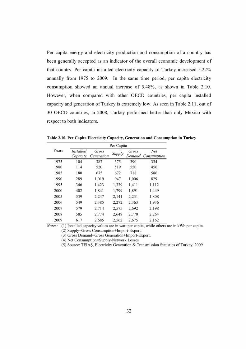
Per capita energy and electricity production and consumption of a country has

been generally accepted as an indicator of the overall economic development of

that country. Per capita installed electricity capacity of Turkey increased 5.22%

annually from 1975 to 2009. In the same time period, per capita electricity

consumption showed an annual increase of 5.48%, as shown in Table 2.10.

However, when compared with other OECD countries, per capita installed

capacity and generation of Turkey is extremely low. As seen in Table 2.11, out of

30 OECD countries, in 2008, Turkey performed better than only Mexico with

respect to both indicators.

Table 2.10. Per Capita Electricity Capacity, Generation and Consumption in Turkey

Per Capita Years Installed

Capacity Gross

Generation Supply Gross Demand

Net Consumption

1975 104 387 375 390 334 1980 114 520 519 550 456 1985 180 675 672 718 586 1990 289 1,019 947 1,006 829 1995 346 1,423 1,339 1,411 1,112 2000 402 1,841 1,799 1,891 1,449 2005 539 2,247 2,141 2,231 1,808 2006 549 2,385 2,272 2,363 1,936 2007 579 2,714 2,575 2,692 2,198 2008 585 2,774 2,649 2,770 2,264 2009 617 2,685 2,562 2,675 2,162

Notes: (1) Installed capacity values are in watt per capita, while others are in kWh per capita. (2) Supply=Gross Consumption+Import-Export. (3) Gross Demand=Gross Generation+Import-Export. (4) Net Consumption=Supply-Network Losses (5) Source: TEİAŞ, Electricity Generation & Transmission Statistics of Turkey, 2009

33

Table 2.11. Per Capita Electricity Capacity, Generation and Supply of OECD Countries in

2008

Per Capita Countries Installed

Capacity Gross

Generation Gross Supply

Australia 2,580 11,957 11,148 Austria 2,494 8,046 7,722 Belgium 1,565 7,927 8,422 Canada 3,830 19,541 17,954 Czech Republic 1,699 8,006 6,242 Denmark 2,277 6,630 6,685 Finland 3,135 14,576 16,403 France 1,838 8,966 7,721 Germany 1,696 7,759 6,952 Greece 1,269 5,667 5,676 Hungary 861 3,984 4,114 Iceland 8,063 51,563 50,000 Ireland 1,667 6,689 6,374 Italy 1,647 5,328 5,669 Japan 2,197 8,474 8,068 Korea 1,643 9,183 8,751 Luxembourg 3,388 7,347 13,673 Mexico 537 2,429 2,351 Netherlands 1,513 6,545 7,251 New Zealand 2,174 10,162 9,791 Norway 6,455 29,916 26,331 Poland 858 4,098 3,683 Portugal 1,485 4,331 5,028 Slovak Republic 1,360 5,360 4,972 Spain 2,052 6,881 6,293 Sweden 3,666 16,199 15,389 Switzerland 2,516 8,949 8,171 Turkey 588 2,791 2,665 U.Kingdom 1,395 6,347 6,173 USA 3,322 14,347 13,641 OECD Mean 2,086 9,031 8,549

Notes: (1) Installed capacity values are in watt per capita, while others are in kWh per capita. (2) Source: IEA Statistics, Electricity Information, 2010 As stated in Section 2.2.3, in Turkey the electricity prices did not increase

between 2003 and 2008. Following the unwelcome increases in January 2008, the

electricity prices reached to 0.139 $/kWh for industry, and to 0.165 $/kWh for

34

residence customers. With these new tariffs, Turkey started to price the industrial

customers slightly more than OECD average, while the residence customers

continue to pay less than OECD average, according to Table 2.12. Looking at the

structure of electricity price in Turkey, we observe from Table 2.13 that

generation cost makes up 64% of electricity price paid by a household in Turkey

in 2008. Generation cost is followed by distribution cost, which is 11% of the

electricity bill (Erdoğdu, 2009).

Table 2.12. Electricity Prices of Some OECD Countries According to OECD Mean in 2008

Countries For Industry Countries For

Residence Korea 0.060 Korea 0.089 Norway 0.064 Mexico 0.096 New Zealand 0.071 Switzerland 0.154 Switzerland 0.094 Greece 0.157 Sweden 0.095 France 0.164 Finland 0.097 New Zealand 0.164 France 0.105 Norway 0.164 Greece 0.112 Turkey 0.165 Poland 0.119 Finland 0.172 Luxembourg 0.123 Czech Republic 0.191 Spain 0.125 Poland 0.193 Mexico 0.126 OECD Mean 0.199 Denmark 0.130 Japan 0.206 Portugal 0.131 Luxembourg 0.215 OECD Mean 0.133 Spain 0.218 Japan 0.139 Sweden 0.218 Turkey 0.139 Portugal 0.220 Belgium 0.140 Slovak Republic 0.220 Netherlands 0.140 Hungary 0.224 U.Kingdom 0.146 U.Kingdom 0.231 Czech Republic 0.151 Netherlands 0.243 Austria 0.154 Austria 0.257 Hungary 0.170 Belgium 0.266 Slovak Republic 0.174 Ireland 0.267 Ireland 0.186 Italy 0.305 Italy 0.290 Denmark 0.396

Notes: (1) All values are in $/kWh. (2) Source: IEA Statistics, Electricity Information, 2010

35

Table 2.13. Cost Structure of Electricity Price Paid by a Household in Turkey in 2008

Cost Type Amount Share (%)

Generation (a) 0.121069 64.07 Transmission (b) 0.004152 2.20 Distribution (c) 0.021417 11.33 Retail Sale (d) 0.001639 0.87 Total (A=a+b+c+d) 0.148277 78.47 Energy Fund (1%) (e) 0.001483 0.78 TRT Share (2%) (f) 0.002966 1.57 Municipality Consumption Tax (5%) (g) 0.007414 3.92 Total (B=e+f+g) 0.011862 6.28 VAT (18%) (C=(A+B)*0.18) 0.028825 15.25 Total (A+B+C) 0.188964 100.00

Notes: (1) All values are in TL/kWh. (2) Source: Erdoğdu (2009)

36

CHAPTER 3

METHODOLOGY AND LITERATURE SURVEY This chapter is devoted to methodologies used in estimating efficiency of firms.

For this aim, firstly the definitions of some important concepts will be presented.

Then, two most popular efficiency measurement techniques, Data Envelopment

Analysis (DEA) and Stochastic Frontier Analysis (SFA), will be discussed and

compared with each other.

3.1. DEFINITIONS

3.1.1. Efficiency

“Efficiency” and “productivity” are two concepts which are used to characterize

firms’ resource utilization performance. These two concepts are often treated as

equivalent in the sense that if firm A is more productive than firm B, then it is

generally believed that firm A is also more efficient. Indeed, they are related, but

fundamentally different concepts. Following Ray (2004), the difference between

them can be shown using an example of two firms producing single-output with

single-input.

Assuming that firm A uses Ax units of the input x to produce Ay units of output

y, and firm B produces By units using Bx units, then the average productiveness

(AP) of these firms are

A

A)A(xyAP (3.1)

37

B

B)B(xyAP (3.2)

The firm with higher average productiveness is called as more productive. It

should be noted that in the simple case with one-input and one-output, one does

not need to know the technology to measure the average productiveness of the

firms. It is enough to have the information about the input and output quantities.

On the other hand, efficiency provides a comparison between a firm’s actual

output and the maximum producible quantity from its observed input.37 For this,

the technology described by a production function should be known to get the

efficiencies of the firms. Suppose that the production function is given by

)(xfy (3.3)

and the maximum output producible from input Ax , and from input Bx are

)( A*A xfy (3.4)

)( B*B xfy (3.5)

For firm A, the output-oriented measure of efficiency is

1*A

AA yyTEo (3.6)

If firm A produced the maximum producible output *Ay from input Ax , its

average productivity will be

A

*A* )A(

xyAP (3.7)

whereas at the observed input-output level, its productivity is

A

A)A(xyAP (3.8)

37 This is just the definition of the “output-oriented technical efficiency”, a type of technical efficiency definitions. More explanations regarding the type of technical efficiencies will be provided in Section 3.1.8.

38

Thus, the output-oriented technical efficiency of firm A can be written

alternatively as

)A()A(

*A

*A

AA*A

AA

APAP

xyxy

yyTEo (3.9)

This relationship suggests that the technical efficiency of a firm is equal to its

productivity divided by the productivity of a hypothetical firm producing the

maximum output possible from the same input quantity. Figure 3.1 illustrates

clearly the difference between productivity and efficiency for our simple case in

which one-output is produced from one-input under decreasing returns to scale.

In figure 3.1, the observed input-output bundles of firms A and B are marked

with . The slopes of the line OA and OB are equal to the average productivity of

firm A and firm B, respectively. To determine the efficiency of the firms, we need

to have the information regarding maximum output, *Ay and *

By , producible from

observed input quantities Ax and Bx . The maximum output producible from an

input level depends on production function defined by underlying technology. The

technical efficiency of firm A producing output Ay with input Ax is

*A

*A

AA*A

AA

of slope of slope0A0A

xyxy

yyTEo (3.10)

Similarly, the technical efficiency of firm B

*B

*B

BB*B

BB

of slope of slope0B0B

xyxy

yyTEo (3.11)

As can be seen from Figure 3.1, the firm A is more productive than firm B while

firm B is more efficient than firm A. Thus, higher productivity does not always

39

A

0

production function

Ax Bx

B

imply greater efficiency. This relationship holds only under constant returns to

scale (CRS).

Figure 3.1. Productivity and Output-Oriented Technical Efficiency

Source: (Ray, 2004)

Leaving the simplified “one-input, one-output case” and starting to study on a

more realistic multi-input, multi-output production technologies, one needs to

represent production technologies by help of a set-theoretic framework. For this

reason, before going into details of the technical efficiencies, we provide

necessary definitions of some important concepts such as technology set, output

set, input set and distance functions.

3.1.2. Technology Set

We use the notation of x and y to denote a N×1 input vector of non-negative real

numbers and a non-negative M×1 output vector, respectively. The technology set

consists of all input-output vectors (x, y) such that x can produce y. Notationally,

*A

*B

Ay

iy *By

By

ix

*Ay

40

yxyx producecan :),(S (3.12)

3.1.3. Output Set

The output set, denoted as P(x), is the set of all output vectors, y, that can be

produced using the input vector, x:

S)( producecan )(P y x, :yyx :yx (3.13)

The output set satisfies the following (Coelli et.al., 2005):

)(P x0 . Nothing can be produced from a given set of inputs, x.

Non-zero output levels cannot be produced from zero levels of inputs.

P(x) satisfies strong disposability of outputs. If yyxy and )(P then

)(P xy .

P(x) satisfies strong disposability of inputs. If y can be produced from x,

then y can be produced from any xx .

P(x) is closed.

P(x) is bounded. One cannot produce unlimited levels of outputs with a

given set of inputs.

P(x) is convex. If two combinations of output levels can be produced with

a given input vector x, then any weighted average of these outputs can also

be produced.

In Figure 3.1, the output set is illustrated for the simple case where two outputs,

1y and 2y , are produced using the input vector, x.

41

Figure 3.2. Output Set

3.1.4. Production Possibility Curve (Output Isoquant)

The boundary of output set is called as production possibility curve or output

isoquant, shown in Figure 3.3. Production possibility curve represents the output

combinations that could be produced using a given input level. One can draw a

production possibility curve for each input level.

Figure 3.3. Production Possibility Curve

1y

2y

Output Set_P(x)

0

IsoqP(x)

1y

2y

0

42

3.1.5. Input Set

The input set, L(y), consists of all input vectors, x, that can produce a given output

vector, y:

S)( producecan )(L y x, :x yx :xy (3.14)

The properties of the input set are as follows:

L(y) is closed for all y.

L(y) is convex for all y.

Inputs are said to be strongly disposable if )(L yx and if xx then

)(L yx .

Figure 3.4 shows the input set when two inputs, 1x and 2x , are used in production

of output vector y.

Figure 3.4. Input Set

1x

2x

Input Set_L(y)

0

43

It should be noted that the output and input set descriptions are the same because

they contain the same information (Coelli, 2005): If y belongs to P(x), i.e. y can

be produced using input vector x, then x belongs to the input set of y, L(y).

3.1.6. Input Isoquant

The boundary of the input set is called as input isoquant, shown in Figure 3.5. The

input isoquant shows the combinations of inputs that could be used to produce a

given output level. Similar to its output counterpart, an input isoquant could be

drawn for each output level.

Figure 3.5. Input Isoquant

Taking into account the time, technical changes may be possible through time. If

the technical advances occur, the production possibilities curve shifts upward,

while input isoquant moves downward. It means that with technical advances,

more output could now be produced using the same input level; or alternatively,

less input is now needed to produce the same output level. A neutral38 technical

change (advance) is illustrated in Figure 3.6.

38 In the case of non-neutral technical change, the technical change favours production of one output (or usage of one input), and thus the shift in the production possibilities curve (or in the input isoquant) will not be parallel.

IsoqL(y)

1x

2x

0

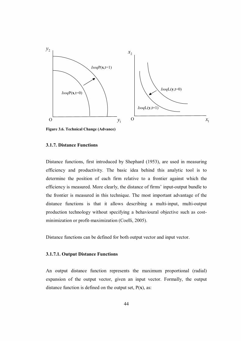
44

1y O 1x O

Figure 3.6. Technical Change (Advance)

3.1.7. Distance Functions

Distance functions, first introduced by Shephard (1953), are used in measuring

efficiency and productivity. The basic idea behind this analytic tool is to

determine the position of each firm relative to a frontier against which the

efficiency is measured. More clearly, the distance of firms’ input-output bundle to

the frontier is measured in this technique. The most important advantage of the

distance functions is that it allows describing a multi-input, multi-output

production technology without specifying a behavioural objective such as cost-

minimization or profit-maximization (Coelli, 2005).

Distance functions can be defined for both output vector and input vector.

3.1.7.1. Output Distance Functions

An output distance function represents the maximum proportional (radial)

expansion of the output vector, given an input vector. Formally, the output

distance function is defined on the output set, P(x), as:

2x

IsoqL(y,t=0)

IsoqL(y,t=1)

2y

IsoqP(x,t=0)

IsoqP(x,t=1)

45

1Ay 1Ay

)P(:min),(O x)(y/ yx d (3.15)

The properties of the output distance function ),(O yxd are as follows (Coelli,

2005):

(i) 0(O x,0)d for all non-negative x.

(ii) ),(O yxd is non-decreasing in y and non-increasing in x.

(iii) ),(O yxd is linearly homogeneous in y.

(iv) ),(O yxd is quasi-convex in x and convex in y.

(v) If y belongs to the output set of x (i.e. )(P xy ), then 1(O y)x,d .

(vi) 1(O y)x,d if y is on the production possibilities curve (namely, on the

frontier of the output set).

Figure 3.7. Output Distance Function and Production Possibility Curve

The notion of the output distance function is demonstrated in Figure 3.7 for the

simple case where two outputs, 1y and 2y , are produced using the input vector x.

O

2Ay

2Ay A C

B

IsoqP(x)

1y

2y

P(x)

46

The output distance measure is the reciprocal the factor by which the production

of all output quantities could be increased while still remaining within the feasible

output set P(x) for the given input level x. Thus, the value of the distance function

for the firm A using input level x to produce outputs 1y and 2y is equal to the

ratio OA/OB , which is less than 1. On the other hand, the firms B and C are

on the production possibilities curve, thus their output distance function values

equal to 1.

3.1.7.2. Input Distance Functions

An input distance function demonstrates the minimal proportional (radial)

contraction of the input vector, given an output vector. It is defined on the input

set, L(y), as:

)L(:max),(I y)(x/ yx d (3.16)

The properties of the input distance function ),(I yxd are as follows (Coelli,

2005):

(i) ),(I yxd is non-increasing in y and non-decreasing in x.

(ii) ),(I yxd is linearly homogeneous in x.

(iii) ),(I yxd is concave x and quasi-concave in y.

(iv) If x belongs to the input set of y (i.e. )(L yx ), then 1),(I yxd .

(v) 1),(I yxd if x is on the input isoquant (namely, on the frontier of the

input set).

Figure 3.8 illustrates the input distance function for the simple case where two

inputs, 1x and 2x , are used in production of output vector, y. The value of the

input distance function for the firm A using A1x of input 1x and A2x of input 2x to

47

1Ax 1Ax

produce output vector y is equal to the ratio OA/OB , which is larger than 1.

On the other hand, since the firms B and C are on the input isoquant, their input

distance functions take the value of 1.

Figure 3.8. Input Distance Function and Input Isoquant

3.1.8. Technical Efficiency

Koopmans (1951) provides the formal definition of technical efficiency as: “a

producer is technically efficient if an increase in any output requires a reduction in at

least one other output, or an increase in at least one input, and if a reduction in any

input requires an increase in at least one other input or a reduction in at least one

output”. However, Farrell’s (1957) seminal work is considered to be the first to

provide a theoretical framework for determination of technical efficiencies.

The technical efficiency is one of two components of a firm’s efficiency,

according to Farrel (1957).39 The level of technical efficiency of a particular firm

39 The other component of the efficiency is allocative efficiency which reflects the ability of the firm to use the inputs in optimal proportions, given their respective prices and the production technology. Technical and allocative efficiency together provide the economic efficiency. Since

O

C

B

A 2Ax

2Ax

IsoqL(y)

1x

2x

L(y)

48

is characterized by the relationship between observed production and some ideal

or potential production (Greene, 1993). The measurement of firm specific

technical efficiency is based upon deviations of observed output from the best

production or efficient production frontier. If a firm's actual production point lies

on the frontier it is perfectly efficient. If it is located inside the frontier then it is

technically inefficient.

The technical efficiency may be expressed in terms of output-oriented or input-

oriented.

3.1.8.1. Output-Oriented Technical Efficiency

In the output-oriented technical efficiency, an answer to the question of “By how

much can output quantities be proportionally expanded without altering the input

quantities?” is searched (Coelli, 2005). In other words, output-oriented technical

efficiency measures the ability of the firm to obtain maximum output for a given

input vector. The output-oriented technical efficiency can be shown by help of

output distance function which is drawn in Figure 3.7. In that figure, the distance

AB is the amount by which all outputs could be proportionally increased without

extra input. In other words, the distance AB is the technical inefficiency of firm A.

Thus, the output-oriented technical efficiency of this firm in terms of ratio is equal

to one minus AB/OB; namely,

OBOATE / (3.17)

As explained in Section 3.1.7.1, the output distance function ),(O yxd is also

equal to the ratio OBOA / . In other words, the output distance function and

this study aims to measure the technical efficiencies of the electricity distribution firms, we give the explanations regarding only technical efficiency.

49

output-oriented technical efficiency take the same value, which is between zero

and one:

OBOAdTE /),(O yx (3.18)

If the firm under consideration (like firm C in Figure 3.7) is on the production

possibility curve, it means that the firm is technically efficient.

3.1.8.2. Input-Oriented Technical Efficiency

In the input-oriented technical efficiency, the question of “By how much can input

quantities be proportionally reduced without altering the output quantities?” is

examined. Figure 3.8 illustrating the input distance function can be used to

explain the input-oriented technical efficiency. The distance AB in Figure 3.8 is

the amount by which inputs could be proportionally decreased without a reduction

in input. Hence, the distance AB provides the technical inefficiency of firm A.

Thus, the input-oriented technical efficiency of this firm in terms of ratio is equal

to one minus AB/OA; namely

OAOBTE / (3.19)

As explained in Section 3.1.7.2, the input distance function ),(I yxd for firm A is

equal to the ratio OBOA / . In other words, input-oriented technical efficiency is

reciprocal of the input distance function:

OAOBd

TE /),(

1

I

yx

(3.20)

The points which are on the input isoquant (like C in figure 3.8) correspond to the

technically efficient cases, with a value of one for the technical efficiency score.

50

3.2. EFFICIENCY MEASUREMENT

As explained in Section 3.1, technical efficiency is defined as the distance of a

firm from an efficient frontier which is accepted as a benchmark. The problem

here is that while one can observe input-output combinations of the firms, the

efficient frontier is not known. For this reason, the efficient frontier should be

firstly determined.

There are several methods of constructing the efficient frontier. These methods

can be categorized according to the assumptions and techniques which are used.

First, the frontier may be determined parametrically or non-parametrically. In

parametric approach, the functional form for the frontier and distribution of the

deviations from it are assumed, and then the frontier is estimated using

econometric techniques. Non-parametric approaches, on the other hand, neither

impose any a priori assumptions about functional form of the frontier nor make

any distributional assumptions for the deviations from the frontier. Instead,

nonparametric approaches rely on linear programming to calculate piecewise

linear segments of the efficient frontier.

Another categorization of the efficiency measurement methods is based on the

structure of the deviations from the frontier. In this respect, the technical

efficiency can be calculated deterministically or stochastically. In the

deterministic approach, the distance between an observed inefficient firm and the

efficient frontier is entirely attributed to the inefficiency. On the contrary, in

stochastic approaches, one can attribute some part of the deviations from the

frontier to random noises.

In the literature, one of the most popular methods in measuring the efficiency of

firms is Stochastic Frontier Analysis (SFA), which is astochastic and parametric

51

method. Among the nonparametric methods, Data Envelopment Analysis (DEA)

has been used widely.

3.2.1. Data Envelopment Analysis (DEA)

Following the proposition in Farrel (1957), Boles (1966) and Shephard (1970)

suggested a linear programming method to determine the efficient frontier as a

piecewise-linear convex hull. However, this mathematical programming method

has gained popularity with Charnes et al. (1978), in which this method was first

named as data envelopment analysis (DEA).

Charnes et al. (1978) suggested an input-oriented approach to measuring

efficiency assuming constant returns to scale (CRS). In the following years, Fare

et al. (1983) and Banker et al. (1984) relaxed the CRS assumption and introduced

the variable returns to scale (VRS) into DEA model.

Now we set out the linear programming problem corresponding to the basic input-

oriented DEA specification of Charnes et al. (1978) under CRS assumption.40 For

this, as a starting point assume that there exist only one output which is produced

from only one input. In this simple case, the efficiency is simply measured as a

ratio between output and input of the relevant i-th firm:41

i

ii input

outputTE (3.21)

However, firms usually produce more than one output using many inputs. Thus, in

such multi-input ix and multi-output iy cases, the inputs and outputs may be 40 Since this study aims to use SFA rather than DEA in measuring technical efficiencies of electricity distribution companies, in this section we find it enough to explain DEA under only Charnes et al. (1978) specification. 41 Although the equation 3.21 is just definition of productivity rather than efficiency, we can use them interchangeably under CRS assumption, as stated in Section 3.1.1.

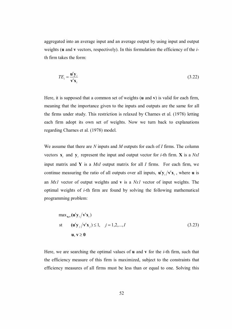
52

aggregated into an average input and an average output by using input and output

weights (u and v vectors, respectively). In this formulation the efficiency of the i-

th firm takes the form:

i

iiTE

xvyu

(3.22)

Here, it is supposed that a common set of weights (u and v) is valid for each firm,

meaning that the importance given to the inputs and outputs are the same for all

the firms under study. This restriction is relaxed by Charnes et al. (1978) letting

each firm adopt its own set of weights. Now we turn back to explanations

regarding Charnes et al. (1978) model.

We assume that there are N inputs and M outputs for each of I firms. The column

vectors ix and iy represent the input and output vector for i-th firm. X is a NxI

input matrix and Y is a MxI output matrix for all I firms. For each firm, we

continue measuring the ratio of all outputs over all inputs, ii xvyu , where u is

an Mx1 vector of output weights and v is a Nx1 vector of input weights. The

optimal weights of i-th firm are found by solving the following mathematical

programming problem:

)max ii xvyu(vu,

st Ijjj 1,2,..., ,1) xvyu( (3.23)

0vu ,

Here, we are searching the optimal values of u and v for the i-th firm, such that

the efficiency measure of this firm is maximized, subject to the constraints that

efficiency measures of all firms must be less than or equal to one. Solving this

53

mathematical programming for each of the I firms, one may determine the most

favourable set of weights for each firm.

It should be noticed that if ) ,( ** vu is a solution to the mathematical

programming given above, then ) ,( ** vu is another solution, meaning that we

face infinite number of solutions (Coelli et.al., 2005). To avoid this problem,

Charnes et al. (1978) imposed the constraint 1 ixv . With this new constraint,

the linear programming takes the form:

)(max , iyμνμ

st ,1 ixν (3.24)

Ijjj 1,2,..., ,0 xνyμ

0ν μ ,

Since this mathematical programming is different from the previous one, we

changed the notation from u and v to μ and ν , as used in Coelli et.al. (2005).

This form of DEA model is known as the multiplier form. Taking its dual, we can

obtain the envelopment form of the DEA model:

λ,min

st ,0 Yλq- i (3.25)

,0 Xλxi

0λ

The envelopment form takes the i-th firm and then seeks to radially contract the

input vector ix , as much as possible, while still remaining in the feasible input

set. Thus, similar to the multiplier form, the envelopment form is also solved for

each of the I firms. In the envelopment form, is the amount of radial reduction

in the use of each input without any change in outputs. Thus, scalar represent

54

technical efficiency of the relevant i-th firm. In this specification, λ is a Ix1

vector of constants.

The inner-boundary of the input set constitutes the piece-wise efficient frontier.

The radial contraction of the input vector ix produces a projected point ( Xλ , Yλ )

on this frontier. This projected point is a linear combination of observed data

points. The constraints of the envelopment form ensure that this projected point

cannot lie outside the feasible set (Coelli et.al. 2005).

As an illustration of the DEA technique, we consider five firms using two inputs,

1x and 2x , to produce one output, y. The linear programming solution produces

piece-wise linear frontier SS , shown in Figure 3.9. Firms which are situated on

this frontier (C, D and E) are fully efficient while firms which lie above-right of

the frontier (A and B) are inefficient.

Figure 3.9. Input-Oriented Efficiency Measurement with DEA

The technical efficiency of firm A is captured by the ratio AA 0/0 . One should

note that the point A in Figure 3.9 does not represent a firm. Point A illustrates

B S

S

A

E

0

D

C

A

yx /1

yx /2

B

55

the position where firm A would occupy if it could be made fully efficient by

radially reducing its use of both inputs.

As illustrated, the input-oriented DEA method calculates efficiency scores by

reducing radially input usage, and in this way moving the firm towards the best

practice frontier suggested by the all other observations.

3.2.2. Stochastic Frontier Analysis (SFA)

It is possible to estimate a production frontier using cross-sectional data on I

firms. For this aim, all data points are enveloped by an arbitrarily-chosen function.

Aigner and Chu (1968) used this approach using a Cobb-Douglass production

frontier of the form:

i

N

nnini uxy

10 lnln (3.26)

where iy is the output of the i-th firm, nix is the n-th input used by i-th firm, ’s

are unknown parameters and iu is a non-negative random variable associated with

technical inefficiency.

Production frontier given in equation 3.26 is deterministic in the sense that all

observed output points iy ’s are bounded from above by a deterministic frontier

of

N

nnin x

10 )lnexp( . Accordingly, these kind of deterministic specifications

exclude the possibility of the measurement error and other sources of statistical

noises, and attribute all deviations from the frontier, ( )exp( iu ) to the technical

inefficiency. This assumption may be problematic especially when statistical

noises are possible due to measurement errors in inputs, nix , specification errors

in production function and any shocks outside the control of the firms. Thus, as an

56

alternative to the deterministic specification, stochastic production frontier is

defined by introducing another random variable representing statistical noise.

Stochastic frontier analysis (SFA) was proposed simultaneously by Aigner et al.

(1977) and Meeusen and van den Broeck (1977). They added a symmetric random

error ( iv ) to the deterministic production frontier in order to account for the

statistical noises:

ii

N

nnini uvxy

10 lnln (3.27)

It is assumed that random error iv independently distributed from technical

inefficiency term iu , and both errors are uncorrelated with the explanatory input

variables nix . In SFA, the frontier,

N

ninin vx

10 )lnexp( , bounding above

the outputs has now a stochastic nature. Since the error term ( iv ) is a random

variable with positive or negative value, the stochastic frontier varies about the

deterministic part of the model,

N

nnin x

10 )lnexp( .

Following Coelli et.al. (2005), we can examine the stochastic frontier model

graphically by help of a Cobb-Douglas frontier function. For the simple case in

which only one input, ix , is used in the production of output iy , Cobb-Douglas

stochastic frontier can be alternatively written as:

iiii uvxy lnln 10 (3.28)

)lnexp( 10 iiii uvxy (3.29)

57

inefficiency effect inefficiency effect

0

deterministic frontier

Ax Bx

)exp()exp()lnexp( 10 iiii uvxy (3.30)

In equation 3.30, )exp( iu takes a value between zero and one and provides us

the technical efficiency of the i-th firm. It measures the output of the relevant firm

relative to the output of a fully-efficient firm using the same amount of inputs:

N

ninin

ii

vx

yTE

10 )lnexp(

(3.31)

N

ninin

N

niinin

i

vx

uvxTE

10

10

)lnexp(

)lnexp(

(3.32)

)exp( ii uTE (3.33)

Figure 3.10 shows such a stochastic production frontier with decreasing returns to

scale.

Figure 3.10. The Stochastic Production Frontier

Source: (Coelli et al., 2005).

iy

By

Ay

*By

*Ay

noise effect noise effect

noise deterministic component

ix

inefficiency

58

In Figure 3.10, the observed output and input combinations of two firms, A and B,

are depicted with . In the absence of inefficiency effects ( 0 BA uu ), the

frontier outputs, which are stochastic, would be

)lnexp( 10*

iii vxy i=A, B. (3.34)

These frontier values are shown with . The stochastic frontier can be above or

below the deterministic frontier when the error term iv is positive and negative,

respectively. The observed outputs are below the deterministic frontier when the

sum of the noise and inefficiency effect is negative ( 0 ii uv ).

In order to determine technical efficiencies using a stochastic production frontier,

one should estimate firstly the parameters of the production frontier in equation

(3.27). However, the stochastic production frontier has a “composed error i ”

including an noise component iv and inefficiency component iu . Thus, it is

necessary to make some assumptions about these error terms. They are as follows

(Coelli et al., 2005):

,0)( ivE (zero mean) (3.35)

,)( 22vivE (homoskedastic) (3.36)

jivvE ji 0)( (uncorrelated) (3.37)

,constant)( 2 iuE (homoskedastic) (3.38)

jiuuE ji 0)( (uncorrelated) (3.39)

As can be seen, the properties of the noise term iv are suitable to apply Ordinary

Least Squares (OLS) technique. However, inefficiency term iu has feature of

0iu , making the composed error term i asymmetric:

59

0)()(0)()()( iiiii uEuEuEvEE (3.40)

Since 0)()( ii uEE , estimation of equation 3.27 by OLS can provide

consistent estimate of n ’s (n=1.2.,,,N), but not of the 0 . The OLS estimator of

the 0 is biased downwards. Also, OLS does not provide estimates of firm-

specific technical efficiency. One solution to this problem is to make additional

assumptions regarding the inefficiency term ( iu ), and to use maximum likelihood

estimation (MLE) technique. The distributions used in the literature for the

inefficiency term ( iu ) are half-normal42, truncated-normal43, exponential44 and

gamma45. Kumbhakar and Lovell (2000) provides the log-likelihood functions for

these different models. Ritter and Simar (1997) suggests that different

assumptions about distributions generally give rise to similar rankings among

firms although technical efficiency scores vary depending on the assumptions

made.

Before maximizing the log-likelihood functions of different models, it is

convenient to reparameterise them. For example, the models we utilize in this

study are based on the Battese and Corra (1977) in which the log-likelihood

function for truncated-normal distribution is reparameterized using 222uv

and 22 / u . The parameter must lie between 0 and 1. If it equals to zero it

means that all deviations from the frontier are due to noise iv ; on the other hand,

the value of one for the parameter means all deviations are because of the

technical inefficiency.46

42 Aigner et al. (1977). 43 Stevensen (1980). 44 Meeusen and van den Broeck (1977). 45 Greene (1993). 46 An alternative reparametresation is due to Aigner et al. (1977) which replaces 2

v and 2u with

222uv and 222 / vu for half-normal model. In this case, a value of zero for

60

Maximizing the the log-likelihood functions, one should set first order derivatives

with respect to unknown parameters to zero. However, first-order conditions are

highly nonlinear and cannot be solved analytically (Coelli et al., 2005). Thus, an

iterative optimization procedure is utilized to estimate the values of the parameters

( ’s, , and - or ) . Judge et al. (1985) provides information on the iterative

optimization procedures.

Obtaining the estimated values of the parameters, the predictor of the inefficiency

component ( iii yuEu ˆ ) should be found. For this aim, conditional pdf,

)( ii yup , is determined in order to see likely and unlikely values of iu after firm i

has been selected and after we have observed its output, iy (Coelli et al., 2005).

Then, the technical efficiency of the i-th firm is found using the predictor value of

iu in the equation )ˆexp( ii uTE .

The explanations made above are regarding the technical efficiency predictions

for a simple production model in which only one type of output is produced. In

the case of multiple outputs, this simple model does not permit the prediction of

the efficiency scores, and one may aggregate the multiple outputs into a single

index of output such as aggregate revenue, or Tornqvist and Fisher index. For

such an aggregation, the prices of the output should be available, and revenue

maximization assumption is required. However, in most of the sectors, the pricing

of the outputs cannot be meaningful; or if so, it is not possible to reach their

prices, or most importantly revenue maximization assumption may not be met.

For such multi-output production technologies, the method of distance functions,

introduced in Section 3.1.7, has been used extensively in the literature. In this

study, we follow this suit and measure the efficiency of electricity distribution

parameter means that there are no technical inefficiency effect and all deviations from the frontier is due to noise.

61

companies by help of distance functions. The explanations regarding SFA models

we utilized in this study will be presented in Section 4.1.

3.2.3. Comparison of DEA and SFA

SFA and DEA are the most common methods used for estimating frontier

functions and thereby measuring technical efficiencies of firms. DEA is based on

linear programming whereas SFA employ econometric techniques. Since these

two techniques are radically different, SFA and DFA methods have their own

strengths and weaknesses. The pros and cons of these methods have been

extensively discussed in the literature.

The main advantage of DEA is that it does not need any restriction on the

functional form of the production relationship between inputs and outputs. In

other words, this method allows the data to “speak for themselves” (Mortimer,

2002). SFA, in contrast, requires strong assumptions regarding the form of the

frontier. Similarly, DEA does not require any assumption for the underlying

distribution of the inefficiency term while SFA imposes distributional assumption

on inefficiency term.

As a result of having no assumptions regarding the form of the frontier and

inefficiency term, DEA is a deterministic method in nature. In other words, all

deviations from the efficiency frontier are assumed to be under control of the firm,

so attributed as inefficiency.47 Another drawback of DEA is that it does not allow

any statistical significance tests. On the contrary, SFA can model the stochastic

shocks by help of the random error introduced into the specification of the

frontier. With SFA one may also carry out statistical tests on different models

with alternative specifications.

47 Several studies have aimed to provide a statistical foundation to DEA. One of these studies is Simar and Wilson (2002) which employ a bootstrapping technique.

62

As emphasized by Jacobs (2000), there exists a sharp trade-off in making a

selection between these two methods. Thus, the literature comparing empirically

and experimentally these two methods is growing extensively.48 The literature

comparing these two methods has no conclusion on which method is more

advanced and correct. In this literature, one can find some suggestions as to

selecting the correct method, although they should be considered just as rule of

thumb in nature. For example, Banker et al. (1993) favoured DEA method where

measurement error is unlikely and the assumptions of the neoclassical production

theory are in question. In contrast, they claimed that econometric methods

performs well when severe measurement errors exist and the underlying

production technology can be illustrated by help of a simple functional form.

We may mention additional strengths and weaknesses of these methods. For

instance, with DEA it is possible to identify “peers” for the inefficient firms, in

this way inefficient firms can compare directly themselves with their efficient

counterparts. However, the efficiency estimations of DEA method is extremely

sensitive to variable selection, size of the sample and data errors. For example, as

more variables are included in DEA models, the number of firms on the frontier

increases. In addition, in DEA at least one of the firms should obtain full

efficiency score, namely 1. This is so because of the fact that DEA only measures

efficiency relative to best practice in the sample studied. For this reason, it is not

meaningful to compare efficiency scores calculated from two different DEA

studies. On the other hand, SFA method usually necessitates estimating a

considerable amount of parameters, some of which may be frequently found

insignificant or even with wrong signs.

48 Mortimer (2002) reviewed systematically the studies comparing these competing methods.

63

CHAPTER 4

MODELS AND DATA In this chapter we first explain the models used in this study in the distance

function framework. In addition, the specification of alternative models set up to

measure efficiency scores of electricity distribution firms is presented. Lastly, the

input, output and environmental variables used in these models are analyzed in

this chapter.

4.1. MODELS

In this study, the models we utilize are based on the concept of distance function.

As explained in Section 3.1.7, distance functions allow describing a multi-input,

multi-output production technology without the need to specify a behavioural

objective such as cost-minimisation or profit-maximisation.

In Turkish electricity market, distribution companies have been responsible from

serving all customers in predetermined regions. In other words, similar to those of

other countries, outputs in Turkish electricity market are accepted as exogenous.

Thus, we measure the input-oriented technical efficiency of electricity distribution

companies by help of input distance function. To be clear, we search an answer to

the question of “By how much can input quantities be proportionally reduced

without altering the output quantities?”. Meanwhile, as explained in Section

3.1.7.2, input-oriented technical efficiency is reciprocal of the input distance

function:

),(1

I yxdTE (4.1)

64

To empirically estimate technical efficiencies with this relationship, one should

first specify a functional form for the input distance. The functional forms with

the following features should be preferred (Coelli and Perlman, 2000): (i) flexible,

(ii) easy to calculate, (iii) suitable for the imposition of homogeneity. The translog

form has these features, and thus extensively used in the literature.49 For this

reason, we also selected the translog form to specify the input-distance function.

The translog input distance function50 for M outputs and N inputs may be

specified as:

N

nnitn

M

mlitmit

M

lml

M

mmitmit xyyyd

11 110 lnlnln

21ln),(ln yx

txyxx t

M

mnitmit

N

nmn

N

nkit

N

knitnk

1 11 1

lnlnlnln21 (4.2)

where i (i=1,2,…,I) denotes the i-th firm in the sample and t (t=1,2,…,T) is time

trend to cover the technical change.

As input-distance function is linear homogeneous in inputs, the parameters in

equation 4.2 must fulfill the following regularity conditions:

N

nn

11 (4.3)

N

knk

10 (4.4)

N

nmn

10 (m=1,2,…,M) (4.5)

49 Coubb-Douglas functional form is another candidate for distance functions. However, Coubb-Douglas form, which is a special case of translog form, is not flexible in the sense that it restricts the elasticity of substitutions. 50 In order to provide clarity in notations, from now on, we will not use the subscription I indicating that the distance function is input-oriented unless it is necessary. Meanwhile, one should note that the notation of I (italic) denotes the number of the firms in the sample.

65

Symmetry is also imposed by the following conditions:

lmml (m, l=1,2,…,M) (4.6)

knnk (n, k=1,2,…,N) (4.7)

Homogeneity in inputs implies that

),(),( II yxyx wdwd , w>0 (4.8)

As suggested by Lovell et al. (1994), selecting one of the inputs arbitrarily (say N-

th input) and setting Nxw /1 , we obtain

MM xdxd /),(),( II yxyx/ (4.9)

With the normalization51, the translog distance function given in equation 4.2 can

be written as follows:

1

1

*

1 110 lnlnln

21ln/),(ln

N

nnitn

M

mlitmit

M

lml

M

mmitmNiit xyyyxd yx

txyxx t

M

mnitmit

N

nmn

N

nkit

N

knitnk

1

*1

1

1

1

*1

1

* lnlnlnln21 (4.10)

where Nitnitnit xxx /* .

This expression can be rearranged as follows:

1

1

*

1 110 lnlnln

21ln)ln(

N

nnitn

M

mlitmit

M

lml

M

mmitmNit xyyyx

ititt

M

mnitmit

N

nmn

N

nkit

N

knitnk uvtxyxx

1

*1

1

1

1

*1

1

* lnlnlnln21 (4.11)

where itv is a random statistical noise and itu is equal to 0),(ln iiitd yx

measuring the technical inefficiency of i-th firm at time t.

51 The operation of deflating N-1 inputs by the N-th input is called normalization.

66

In practice, it has been assumed that the random statistical noise itv has the

standard features, it is an independently and identically distributed (iid) random

error term ( itv ~ iid N(0, 2v )). As for inefficiency term itu , however, different

assumptions have been used in literature, and based on these assumptions,

different models have been produced. Among them, we utilized BC92&BC95,

both of which are classified as time-varying inefficiency models. In other words,

these models let the technical efficiency scores change over time.

The elasticities of the input distance function ),(ln yxitd with respect to inputs

and outputs provide valuable information52: Firstly, for cost-minimising levels of

inputs, the elasticity of input distance function with respect to an input nitx , nit ,

equals to cost share of the n-th input for i-th firm at time period t, nits ;

nit

itnit x

dln

),(ln

yx (4.12)

nitmit

M

mmn

N

kkitnkn syx

lnln11 (4.13)

Therefore, elasticity nit provides information about the relative importance of the

n-th input (Rasmussen 2010).

Similarly, for cost-minimising levels of inputs, the elasticity of input distance

function with respect to an output mity , mit , equals to the negative of the

elasticity of cost with respect to the m-th output;

mit

itmit y

dln

),(ln

yx (4.14)

N

nnitmnlit

M

lmlm xy

11lnln (4.15)

52 For the derivation of the following elasticities, see Fare and Primont (1995).

67

In this study, we divide all output and input variables by their respective overall

sample means, which does not change the efficiency scores obtained, but allow

one to interpret the estimated first-order parameters , n and m , directly as

elasticities, nit and mit respectively, evaluated at the sample means

(Rungsuriyawiboon and Coelli 2004).

Meanwhile, the sum of the elasticities of input distance function with respect to

outputs provides the the degree of returns to scale (RTS);

M

mmitRTS

1 (4.16)

If the RTS is less than unity in absolute value, it means that the production

technology has increasing returns. In contrast, if the RTS is larger than unity, then

the production technology has decreasing returns to scale. The RTS with the value

of unity indicates the constant returns (Goto and Tsutsui 2008).

It is also possible to calculate the technological change (TC) or shift in the

production frontier over time;53

tit

tdTC

),(ln yx (4.17)

If TC is found to be positive, it means that there exists a technological progress in

production. A negative TC, in contrast, indicates technological backwardness.

4.1.1. Battese and Coelli (1992)

BC92 assumes that inefficiency term itu is an exponential function of time. In

other words,

53 For a graphical representation of technological change in the production frontier, see Figure 3.6.

68

))(exp( Ttuu iit , i=1,2,…,N; t=1,2,…,T (4.18)

where iu is firm specific inefficiency terms assumed to be a iid nonnegative

truncated normal distribution, namely iu ~ ) ,( 2uNiid , and is an unknown

parameter to be estimated. Since this model has just one unknown parameter, it is

rather inflexible in comparison to similar models.54 Another limitation of this

model is that it does not allow for a change in the rank ordering of firms over time

although the efficiency scores of the firms change. In other words, the firm that is

ranked n-th at the first time period is always ranked n-th (Coelli et. al. 2005).55

BC92 suggests that the minimum-mean-squared-error predictor of the technical

efficiency ( itTE ) of the i-th firm in the time period t is equal to the expectation of

)exp( itu conditional on the composed error term itit uv :

itititit uvuETE )exp( (4.19)

In this study, we produced three alternative BC92 model specifications using

different input variables and a time trend. The detailed explanations regarding

these alternative specifications can be found in Section 4.2.

4.1.2. Battese and Coelli (1995)

BC92’s restriction that the rank ordering of firms over time does not change may

turn out to be an important drawback especially when there exist several factors

(sometimes called “environmental variables”) which may affect efficiencies of the

firms differently. For example, if some of the firms were privatized during the

time period examined, then it would be logical to expect that the efficiencies of

these firms would increase more than those of other non-privatized companies. To 54 For example, Kumbhakar (1990) assumes a similar but a little more flexible structure for inefficiency term itu . Accordingly, 12 )exp(1

btatuu iit in which a and b are unknown parameters to be estimated. 55 The same limitation is valid for other similar studies such as Kumbhakar (1990).

69

overcome this potential problem, the authors of BC92 introduced another model

(BC95) which let not only inefficiency term itu but also the ranking of the firms

change over time.

BC95 assumes that inefficiency term itu is a iid nonnegative truncated normal

distribution, itu ~ ) ,( 2uitNiid , where

H

hhithit z

10 (4.20)

In this specification, hitz is the h-th exogenous environmental variable which is

expected to determine the firm-specific efficiency itu by affecting the mean of its

distribution it . In addition, h (h=1, 2, …, H) are slope parameters to be

estimated. Negative parameters indicate that the variables of these parameters

improve efficiency; in contrast, if one finds the sign of the some of these

exogenous variables positive, it implies that these variables decrease the

efficiency.

Similarly to BC92, we generated three different models based on BC95. These

alternative model specifications are also explained in Section 4.2 in detail.

Meanwhile, in this study, all model estimates were obtained by maximum

likelihood estimation techniques. We used the software program FRONTIER 4.1.,

which was written by Tim Coelli.

70

4.2. MODEL SPECIFICATIONS AND DATA

The first job in efficiency measurement studies is to determine the inputs, outputs

and other (environmental) factors of the relevant sector. Although electricity

distribution technologies are similar all over the world, a wide variety of factor

combinations are employed in the efficiency studies of this sector.56 In other

words, a variable has been used as input, output or environmental variable in

different studies.57 The absence of consensus on which variables should be used as

input, output or environmental variable may be explained, to some extent, by lack

of data (Hattori et al., 2005).

Before introducing our models and variables, we should underline several

important points: First, it is certainly desirable to take many factors and variables

into account in the efficiency studies. However, in practice there are several

reasons for limiting the number of variables used. First of all, degrees of freedom

problem prevent taking all variables into account, especially when flexible models

such as translog are used in the estimation. Second, when too many factors are

included into model, some of them are probably found to be highly correlated,

leading the problem of multicollinearity. Last, the difficulties of data collection

may cause to limit the number of variables.58

Other important point to be addressed is that in this study we aimed to measure

technical efficiency by using only physical measures of the variables. If the price

data is available and it is reasonable to assume a behavioral objective such as cost

minimization, it is possible (even preferable) to predict cost efficiency using a cost

frontier. Although we have price data for the variables used in this study, we

56 Jamasb and Pollitt (2001) reviewed 20 efficiency studies regarding electricity distribution sector, and showed that there is no firm consensus in the literature on which variables best describe the performance of electricity distribution units. 57 As can be seen from Table 3.1, the efficiency studies of Turkish electricity distribution sector also exhibit a wide variety in the input-output selection. 58 Since we have a rather extensive data set, the last reason is not so valid for our study.

71

prefer not to predict cost efficiency because of the fact that cost minimization

assumption is very questionable in regulated markets such as electricity

distribution sectors mainly due to political and regulatory interventions

(Rungsuriyawiboon and Coelli 2004).

Now we may begin to introduce our models and variables used. Utilizing BC92

we firstly built a base model called BC92-1 with two outputs and three inputs.

Then we extended it twice by adding one input at a time to analyze the effects of

the added variable on overall efficiency. We called the extended BC92 models as

BC92-2 and BC92-3.

In addition to input and output variables, there are obviously other environmental

factors, which can affect the efficiency of the electricity distribution firms. We

took into account environmental factors which are not under the control of the

relevant firms by generating three alternative BC95 models. Our BC95 models are

based on the most extended version of the BC92 models, namely BC92-3. To be

more precise, we created three BC95 models (BC95-1, BC95-2 and BC95-3) by

adding to BC92-3 model one environmental variable at a time. The alternative

model specifications are shown in Table 4.1.

Our base model BC92-1 and its five extensions have two outputs, electricity

delivered in MWh, 1y and number of customers , 2y . The reason for using number

of customer in addition to electricity delivered is that a large part of distribution

activities (metering services, customer connections, billing etc.) are directly

correlated to the number of customers. Thus, when electricity delivered is used as

the only output variable, there exist the risk of unfairly discriminating against

those firms which sell smaller amounts of electricity per customer. Meanwhile,

according to the extensive review by Jamasb and Pollitt (2001), these two

72

variables are the most frequently used outputs in 20 benchmarking studies

reviewed.59

Table 4.1. Specification of Models

Models Variable

BC92-1 BC92-2 BC92-3 BC95-1 BC95-2 BC95-3 y1 Electricity delivered √ √ √ √ √ √

y2 Number of customers √ √ √ √ √ √

x1 Number of employees √ √ √ √ √ √

x2 Length of distribution line √ √ √ √ √ √

x3 Transformer capacity √ √ √ √ √ √

x4 Outage hours per customer √ √ √ √ √

t Time √ √ √ √

z1 Customer density √ √ √

z2 Customer structure √ √

t Time √

In the base BC92-1 model, the number of employees, 1x , the length of the

distribution line in km , 2x and transformer capacity in MVA , 3x are used as input

variables. With number of employees we aimed to approximate the labor input.

Capital input was taken into account by other two variables, the length of the

distribution line and transformer capacity. These three variables have been

similarly found to be the most widely used input variables in Jamasb and Pollitt

(2001).

The first extended model BC92-2 includes the quality of electricity distribution,

4x as an input variable in addition to those of base model BC92-1. The quality of

electricity distribution is generally used as input in efficiency studies.60 Appa et al.

(2010) examined the quality of electricity distribution in detail. Accordingly, the

59 Neuberg (1977) suggested “separate marketability of components” property in defining outputs. Since electricity delivered and number of customers have this property, in literature they are routinely chosen as output variables, if the necessary data is available. 60 Coelli et.al. (2008), Growitsch et.al. (2009) and Bağdadioğlu and Senyücel (2010) are the studies which used quality of electricity distribution as input. This variable is, in contrast, used as an output by Appa et al. (2010).

73

quality of electricity distribution may be separated into two broad categories:

technical quality and quality of customer service (ability to meet customers’ needs

such as new connections or repairs). Technical quality may be measured in terms

of interruption of service or regularity in the voltage level supplied. Frequency of

outages and duration of outages provide the technical quality in terms of

interruption of service. For Turkish electricity distribution market, information

regarding both the number of outages and their total duration is available.

Following Growitsch et al. (2009), we prefer to use the average duration of

blackouts per customer as a proxy for service reliability.61

The third model BC92-3 is created by adding a time trend ,t as an input variable

into BC92-2 model. In so doing, we aimed to capture the technological changes or

frontier shifts, if any.

As stated above, we created alternative BC95 models by adding environmental

variables into the most extended BC92 model, namely BC92-3. Although these

added environmental variables affect efficiencies of the firms, they are beyond

managerial control of the relevant firms. These environmental variables are

directly used for explaining the mean inefficiency term it .

The first BC95 model (BC95-1) includes an environmental variable 1z to account

for the differences in the customer densities of regions (measured in number of

customers per km of distribution line). One may expect that increasing customer

density leads to higher technical efficiency, holding other things equal.

In BC95-2 model, another environmental variable regarding the customer

structure 2z is taken into account (proportion of sales in MWh to residential

61 Similarly, Bağdadioğlu and Senyücel (2010) also used the average outage duration per consumer for the quality variable. Coelli et al. (2008), on the other hand, prefer to use total number of outages for this input variable.

74

customers to total sales). In contrast to the customer density, we do not pose a

priori expectations on the effect of the customer structure on the efficiency

estimation. However, several studies such as Hirschhausen et al. (2006) reported

that an increase of the share of industrial customers represents a disadvantage for

the electricity distribution companies in terms of efficiency.

In addition to these environmental variables, we used in Model 95-3 a time trend t

to explain the changes in the mean inefficiency term it .

Meanwhile, our data set explained above involves annual data on 21 electricity

distribution firms over the eight-year period from 2002 to 2009. This data is

obtained from the web page of TEDAŞ. Descriptive statistics over the variables

are shown in Table 4.2. The mean values of the variables for each distribution

firm over the period examined are given in Table 4.3. As can be seen from this

table, Boğaziçi is the largest electricity distribution firm with respect to both

output variables, electricity delivered and number of customers. This firm is

followed by Toroslar with regard to electricity delivered, and by Başkent with

regard to number of customers.

75

Table 4.2. Descriptive Statistics

Descriptive Statistics Variable Description Unit Mean Minimum Maximum Median Std.Dev.

y1 Electricity delivered MWh 6,105,994.0 1,382,135.0 21,300,000.0 4441497 4,609,341.0 y2 Number of customers person 1,348,031.0 320,639.0 3,886,951.0 1197765 828,941.3 x1 Number of employees person 1,391.5 493.0 4,042.0 1223.5 652.6 x2 Length of distribution line km 39,348.8 12,801.0 95,271.0 37083.5 18,708.44 x3 Transformer capacity MVA 4,437.4 868.0 13,244.0 4050 2,922.1 x4 Outage duration per customer hour/customer 0.042 0.002 0.202 .0319 .0354 z1 Customer density customer/km 38.3 14.9 130.8 27.4 28.5 z2 Customer structure % 28.0 10.8 46.0 27.5 9.0

75

76

Table 4.3. Descriptive Statistics_Mean values over the period 1992-1999

Outputs Inputs Enviro.Variables y1 y2 x1 x2 x3 x4 z1 z2 Akdeniz 4,880,183.9 1,272,226.4 1,091.3 48,412.5 4,200.9 0.015 26.2 0.263 Aras 2,014,846.6 661,074.6 1,494.8 39,069.3 1,518.8 0.083 16.9 0.413 AYEDAŞ 7,596,034.6 1,919,549.9 1,976.6 15,892.6 5,106.9 0.011 120.6 0.423 Başkent 9,749,431.1 2,753,702.0 3,044.3 81,451.5 8,546.1 0.055 33.8 0.326 Boğaziçi 18,443,143.0 3,459,975.5 1,899.1 29,297.1 11,802.8 0.014 118.0 0.334 Çamlıbel 1,842,603.8 681,132.1 919.5 30,398.1 1,571.4 0.017 22.4 0.320 Çoruh 2,090,649.9 916,081.1 1,125.5 42,181.1 1,700.9 0.052 21.7 0.426 Dicle 11,754,074.0 921,164.6 1,768.9 37,580.3 4,773.8 0.122 24.6 0.263 Fırat 2,052,389.3 603,790.9 1,206.9 32,971.9 1,648.6 0.037 18.3 0.277 Gediz 11,883,492.0 2,190,529.0 1,554.5 37,418.3 8,089.6 0.034 58.7 0.247 Göksu 2,969,988.4 438,268.3 652.3 16,507.8 1,577.0 0.095 26.6 0.161 KCETAŞ 2,058,853.8 469,141.1 625.3 14,644.5 1,693.5 0.013 32.0 0.215 Menderes 4,873,664.3 1,331,714.8 921.1 55,792.5 4,889.6 0.034 23.8 0.273 Meram 4,974,487.1 1,384,797.4 1,924.1 55,462.6 5,719.6 0.040 25.0 0.226 Osmangazi 4,137,207.5 1,157,794.4 1,043.5 30,506.8 3,790.8 0.022 37.9 0.208 Sakarya 6,331,141.0 1,232,741.5 1,006.5 36,818.9 5,653.5 0.028 34.0 0.154 Toroslar 12,118,692.0 2,436,088.4 2,423.1 69,691.3 7,956.3 0.029 34.9 0.238 Trakya 4,265,767.4 701,327.0 569.3 13,971.5 2,967.1 0.042 50.2 0.163 Uludağ 8,306,224.3 2,063,678.6 1,555.1 46,591.8 6,040.3 0.019 44.2 0.222 Vangölü 2,176,295.9 361,626.9 946.9 23,334.5 1,123.3 0.050 15.5 0.380 Yeşilırmak 3,706,695.4 1,352,253.6 1,473.3 68,330.8 2,814.6 0.073 19.8 0.359

76

77

The graphs showing the development of the variables over time are presented in

Appendix A. For all firms, a continuous increasing trend is observed in both

output variables (electricity delivered and number of customers) over this period.

As for the input variables, the number of employees shows a decreasing trend in

all firms while length of distribution line and transformer capacity usually

increase over the entire period. On the other hand, the data of other input

variable, outage duration per customer, does not reveal any clear structural

tendency. Examining the graphs of the environmental variables of the firms,

Boğaziçi and AYEDAŞ attract our attention especially with respect to customer

density. The number of customers per km of distribution line is extensively

greater in both side of İstanbul than those of other regions.

78

CHAPTER 5

ESTIMATION RESULTS

In this chapter, efficiency estimation results of alternative models studied are

presented. In addition, comparing the results of these models, we attempt to draw

some robust conclusions in the light of these results.

5.1. ESTIMATION RESULTS FOR ALTERNATIVE BC92 MODELS

The parameter estimates of the input distance function for alternative BC92

models (BC92-1, BC92-2 and BC92-3) are presented in Table 5.1. Given that we

normalized each variable by its sample mean and then used their natural

logarithm, the first-order coefficients ( m , n ; m=1,..,M; n=1,…,N) can be

directly interpreted as elasticities at the sample mean. As explained in Section 4.1,

input elasticities provide information regarding input contribution shares.

First of all, the estimated parameters of the input distance function should satisfy

regularity condition in the sense that the distance function is decreasing in outputs

and increasing in inputs. In other words, the first-order coefficients of the outputs

m and inputs n should take negative and positive values, respectively.62

62 A negative coefficient implies a decrease in input distance function, meaning that an expansion in the input set. In contrast, a positive coefficient implying an increase in the distance function corresponds to a contraction of the feasible input set.

79

Table 5.1. Estimation Results of Alternative BC92 Models

Model BC92-1 Model BC92-2 Model BC92-3 Variable Param.

Coefficient t-ratio Coefficient t-ratio Coefficient t-ratio

Constant 0 0.422*** 7.33 0.414*** 7.26 0.395*** 6.82

1ln y 1 -0.118*** -3.60 -0.145*** -3.66 -0.154*** -4.15

2ln y 2 -0.397*** -9.39 -0.361*** -7.94 -0.390*** -8.78 2

1)(ln y 11 -0.169 -1.30 -0.226 -1.63 -0.126 -0.92 2

2 )(ln y 22 0.477*** 3.20 0.536*** 3.22 0.521*** 3.11

))(ln(ln 21 yy 12 0.102 0.85 0.071 0.53 0.025 0.19

1ln x 1 0.213 - 0.189 - 0.202 -

2ln x 2 0.531*** 13.64 0.546*** 12.70 0.546*** 13.16

3ln x 3 0.256*** 6.63 0.253*** 5.95 0.238*** 5.87

4ln x 4 - - 0.012 1.28 0.014 1.52 2

12 )/(ln xx 22 0.297*** 2.85 0.389*** 3.70 0.347*** 3.12 2

13 )/(ln xx 33 0.003 0.03 -0.002 -0.02 -0.016 -0.15 2

14 )/(ln xx 44 - - 0.015 1.48 0.015 1.39

)/)(ln/(ln 1312 xxxx 23 -0.065 -0.67 -0.113 -1.17 -0.073 -0.72

)/)(ln/(ln 1412 xxxx 24 - - -0.029* -1.76 -0.023 -1.44

)/)(ln/(ln 1413 xxxx 34 - - 0.030* 1.80 0.026 1.55

)/)(ln(ln 121 xxy 12 -0.197*** -3.32 -0.185** -2.60 -0.162** -2.36

)/)(ln(ln 131 xxy 13 0.188** 2.16 0.229** 2.37 0.168* 1.83

)/)(ln(ln 141 xxy 14 - - -0.021 -1.00 -0.020 -0.95

)/)(ln(ln 122 xxy 22 0.241*** 3.49 0.192** 2.50 0.163** 2.13

)/)(ln(ln 132 xxy 23 -0.256*** -3.03 -0.228** -2.56 -0.170* -1.95

)/)(ln(ln 142 xxy 24 - - 0.010 0.43 0.016 0.66

t t - - - - 0.008*** 2.74

Variance 2 0.035*** 11.30 0.033*** 10.77 0.037*** 11.42

Variance ratio 0.975*** 188.3 0.975*** 157.3 0.979*** 232.7

0.367*** 7.09 0.356*** 6.51 0.382*** 7.42

0.003 0.54 0.004 0.67 -0.004 -0.52 Log-likelihood 281.295 282.799 285.511

Notes: (1) ***, ** and * denote significance at the 1%, 5% and 10% level using a two-tailed test. (2) 1 is calculated by homogeneity conditions.

80

Looking at estimated parameters of two first-order output coefficients, 1 and 2 ,

it can be seen that they have the negative sign as expected, and are statistically

significant at 1% significance level, in all three alternative models. We also

observe that alternative models provided rather similar estimated values for each

1 and 2 output parameters. In addition, the sum of first-order output

coefficients is less than 1 in absolute value in all alternative models (0.52, 0.51,

0.54, respectively), indicating the presence of increasing returns to scale at the

mean of the data. To be more precise, for increasing both outputs by 1%, we need

to increase the input requirements only about by 0.5%.

As for the estimated first-order input coefficients, the results show that they have

positive signs as expected across all models. Among them, those of length of

distribution line ( 2 ) and transformer capacity ( 3 ) are statistically significant at

the 1% significance level.63 In addition, the magnitudes of these coefficients differ

slightly across the alternative models. Accordingly, when these first-order input

coefficients are interpreted as cost share, we can conclude that expenses for

distribution line account for slightly more than half of the total costs at the sample

mean. Expenses for the transformers and employees approximately account for

25% and 20% of total costs, respectively.

As explained in Section 4.2, the quality variable defined as outage duration per

customer has been taken into account in Model BC92-2 and Model BC92-3.

Although in both models, the sign of the quality variable is positive as expected;

its value is not statistically significant. It means that introducing the quality

variable into the analysis has no statistically significant effect on the estimated

efficiency scores.

63 Since the coefficient for number of employees ( 1 ) is calculated by homogeneity conditions, its significance test has not be done. Nevertheless, its estimated value is rather high, which lead us to conclude that this input is also important.

81

In searching technical change (TC) in the production frontier over time, a time

trend is included into Model BC92-3. As shown in equation 4.17, the coefficient

of this time trend t provides the shift in the production frontier if any. This

coefficient has been found positive (0.008) and statistically significant at 1%

significance level. This indicates that the production frontier exhibits a

technological progress of 0.8% per year over the period studied.

In all three alternative specifications of BC92, the variance parameters, 2 and

, are statistically significant at 1% significance level.64 The estimated value of

parameter is approximately found 0.98 in all alternative models, indicating that

the variance of the composed error term 2 is attributed to almost entirely the

variance of the technical inefficiency term 2u . In other words, the technical

inefficiency component ( 2u ) dominates the random noise component 2

v , which

makes the usage of deterministic distance functions instead of stochastic ones

plausible.

As for parameter in the exponential model of BC92, defined by equation 4.18,

Model BC92-1 and Model BC92-2 provide positive estimates while Model BC92-

3 calculates a negative estimate.65 However, these estimated values of the

parameter are statistically insignificant, meaning that there is no significant

change in the technical efficiency scores through time, according to alternative

BC92 models.

64 2 and are reparameterized coefficients equivalent to 22

uv and 22 / u , respectively. As explained in Section 3.2.2, these reparameterizations are necessary for maximizing the likelihood function. 65 As explained in Section 4.1.1, positive/negative estimates correspond to increases/decreases in the technical efficiency scores over time.

82

Table 5.2. Technical Efficiency Scores for Model BC92-1

Efficiency Scores Company Rank 2002 2003 2004 2005 2006 2007 2008 2009

Akdeniz 12 0.609 0.610 0.611 0.612 0.614 0.615 0.616 0.617 Aras 17 0.517 0.519 0.520 0.521 0.523 0.524 0.525 0.527 AYEDAŞ 2 0.928 0.928 0.929 0.929 0.929 0.929 0.930 0.930 Başkent 21 0.404 0.405 0.406 0.408 0.409 0.411 0.412 0.414 Boğaziçi 6 0.720 0.721 0.722 0.723 0.724 0.725 0.726 0.726 Çamlıbel 10 0.663 0.664 0.665 0.666 0.668 0.669 0.670 0.671 Çoruh 13 0.588 0.589 0.590 0.591 0.593 0.594 0.595 0.596 Dicle 11 0.627 0.628 0.630 0.631 0.632 0.633 0.634 0.635 Fırat 14 0.556 0.558 0.559 0.560 0.562 0.563 0.564 0.566 Gediz 5 0.734 0.735 0.736 0.737 0.737 0.738 0.739 0.740 Göksu 7 0.711 0.712 0.713 0.714 0.715 0.716 0.717 0.717 KCETAŞ 3 0.815 0.816 0.817 0.817 0.818 0.819 0.819 0.820 Menderes 15 0.550 0.552 0.553 0.554 0.556 0.557 0.558 0.560 Meram 18 0.496 0.497 0.499 0.500 0.501 0.503 0.504 0.506 Osmangazi 4 0.807 0.808 0.808 0.809 0.810 0.810 0.811 0.812 Sakarya 8 0.706 0.707 0.708 0.709 0.710 0.711 0.712 0.713 Toroslar 19 0.491 0.493 0.494 0.495 0.497 0.498 0.500 0.501 Trakya 1 0.992 0.992 0.992 0.992 0.992 0.992 0.992 0.992 Uludağ 9 0.671 0.672 0.673 0.674 0.675 0.676 0.677 0.678 Vangölü 16 0.520 0.521 0.522 0.524 0.525 0.526 0.528 0.529 Yeşilırmak 20 0.462 0.463 0.465 0.466 0.468 0.469 0.470 0.472 Mean 0.646 0.647 0.648 0.649 0.650 0.651 0.652 0.653

The year-by-year technical efficiency predictions of alternative BC92 models

(BC92-1, BC92-2 and BC92-3) are presented in Table 5.2, Table 5.3 and Table

5.4, respectively. As a result of BC92 specification, the rankings of the

companies do not change although their efficiency scores change over the periods.

Since Model BC92-1 and Model BC92-2 estimate positive but insignificant

values for parameter , the efficiency scores of all companies show a slight

increase during 1992-1999 period in these models. In contrast, with a negative

and insignificant estimate for parameter , Model BC92-3 indicates minor

efficiency decreases during the same time period.

83




84




Table 5.5 presents the average efficiency scores for each company over the eight-

year period for alternative BC92 models. In all three alternative models, Trakya is

the most efficient electricity distribution company with an efficiency score of 0.99

approximately. The second most efficient company is AYEDAŞ, according to all

alternative models. Model BC92-1 determines KCETAŞ as the third most

efficient company, while Osmangazi is the third most efficient company

according to Model BC92-2 and Model BC92-3. As for the most inefficient

company, all three models point Başkent with an approximate efficiency score of

0.41, which is somewhat unexpected result. It implies that the same output

quantities could have been produced by Başkent even when the input usage was

reduced by 59% approximately. Yeşilırmak appears as the second most inefficient

85

electricity distribution company, according to all alternative model specifications.

The third most inefficient company is Toroslar according to Model BC92-1 and

Model BC92-2, while Model BC92-3 concludes that the third most inefficient

company is Vangölü. Table 5.5. Average Efficiency Scores for Alternative BC92 Models

Average Efficiency Scores Company BC92-1 BC92-2 BC92-3

Akdeniz 0.613 0.613 0.602 Aras 0.522 0.531 0.495 AYEDAŞ 0.929 0.939 0.937 Başkent 0.409 0.409 0.416 Boğaziçi 0.723 0.734 0.772 Çamlıbel 0.667 0.665 0.628 Çoruh 0.592 0.607 0.569 Dicle 0.631 0.600 0.595 Fırat 0.561 0.562 0.529 Gediz 0.737 0.731 0.751 Göksu 0.714 0.718 0.688 KCETAŞ 0.818 0.769 0.771 Menderes 0.555 0.559 0.544 Meram 0.501 0.498 0.490 Osmangazi 0.809 0.792 0.785 Sakarya 0.710 0.696 0.701 Toroslar 0.496 0.492 0.502 Trakya 0.992 0.984 0.988 Uludağ 0.675 0.673 0.680 Vangölü 0.524 0.531 0.490 Yeşilırmak 0.467 0.483 0.463 Table 5.6 tabulates the summary statistics of technical efficiency scores obtained

by alternative BC92 models. As shown in this table, all three models provide

similar statistics for the efficiency scores: In all models, the efficiency scores vary

from 0.41 to 0.99 approximately while their average is equal to about 0.64. An

obvious reason for the similarity between estimated efficiency scores is that one

86

of the input variables (the quality variable) included into the model specifications

has been found to be lack of power to affect efficiency scores.66

Table 5.6. Summary Statistics of Technical Efficiency Scores for Alternative BC92 Models

Summary Statistics Model Mean Minimum Maximum Median Std. Dev.

BC92-1 0.650 0.404 0.992 0.632 0.149 BC92-2 0.647 0.405 0.984 0.613 0.144 BC92-3 0.638 0.411 0.988 0.603 0.152

5.2. ESTIMATION RESULTS FOR ALTERNATIVE BC95 MODELS

Table 5.7 tabulates parameter estimates of the input distance function for

alternative BC95 models (BC95-1, BC95-2 and BC95-3). Similar to the BC92

applications given in the previous section, since each variable is normalized by its

sample mean and their natural logarithm is used, one may directly interpret the

first-order coefficients ( m , n ; m=1,..,M; n=1,…,N) as elasticities at the sample

mean.

As stated before, the input distance function should be decreasing in outputs and

increasing in inputs. The results confirmed that the input distance functions

estimated using alternative BC95 models has fulfilled this condition at the sample

mean: All the parameter estimates have the appropriate sign ( 0m for all m

outputs and 0n for all n inputs). In addition, they are found to be statistically

significant at the 1% significance level in all models.

66 Taking alternative BC95 models into account as well, a more systematic comparison between all alternative models will be made in Section 5.3.

87

Table 5.7. Estimation Results of Alternative BC95 Models

Model BC95-1 Model BC95-2 Model BC95-3 Variable Param.

Coefficient t-ratio Coefficient t-ratio Coefficient t-ratio

Constant 0 0.128*** 4.36 0.126** 2.56 0.160*** 4.89

1ln y 1 -0.241*** -2.96 -0.332*** -3.39 -0.266*** -4.49

2ln y 2 -0.64*** -7.05 -0.581*** -4.49 -0.669*** -9.63 2

1)(ln y 11 -0.398*** -2.9 -0.410** -2.31 -0.474*** -3.48 2

2 )(ln y 22 0.159 0.65 0.218 1.14 0.179 1.02

))(ln(ln 21 yy 12 0.063 0.36 0.011 0.07 0.058 0.43

1ln x 1 0.19 - 0.19 - 0.158 -

2ln x 2 0.237*** 2.75 0.1 0.83 0.19** 2.52

3ln x 3 0.573*** 7.56 0.698*** 8.93 0.645*** 13.44

4ln x 4 0.000 0.01 0.012 0.50 0.007 0.35 2

12 )/(ln xx 22 0.643*** 6.2 0.419*** 4.02 0.480*** 5.33 2

13 )/(ln xx 33 -0.239** -2.0 -0.424*** -3.41 -0.434*** -3.80 2

14 )/(ln xx 44 0.05** 2.0 0.062** 2.33 0.056** 2.59

)/)(ln/(ln 1312 xxxx 23 -0.353*** -3.81 -0.119 -1.30 -0.183* -1.97

)/)(ln/(ln 1412 xxxx 24 -0.104*** -3.04 -0.121*** -3.15 -0.107*** -3.66

)/)(ln/(ln 1413 xxxx 34 0.067** 2.04 0.073** 2.18 0.069** 2.58

)/)(ln(ln 121 xxy 12 -0.097 -0.97 -0.181* -1.77 -0.143 -1.33

)/)(ln(ln 131 xxy 13 0.404*** 3.81 0.469*** 4.34 0.436*** 3.83

)/)(ln(ln 141 xxy 14 -0.071 -1.39 -0.079 -1.58 -0.072* -1.79

)/)(ln(ln 122 xxy 22 0.186 1.53 0.185 1.53 0.103 0.80

)/)(ln(ln 132 xxy 23 -0.163** -2.04 -0.155* -1.87 -0.111 -1.30

)/)(ln(ln 142 xxy 24 0.062 1.06 0.059 1.06 0.057 1.23

t t 0.006 1.65 0.004 0.79 0.006 1.45

Variance 2 0.01*** 3.77 0.013*** 2.92 0.012*** 5.28

Variance ratio 0.911*** 12.97 0.955*** 22.78 0.978*** 47.89

Constant 0 0.45*** 4.88 0.581** 2.49 0.583*** 10.52

1z 1 -0.009*** -3.94 -0.009 -1.53 -0.01*** -13.32

2z 2 - - -0.797*** -3.68 -0.736*** -3.64

3z 3 - - - - 0.015 1.50 Log-likelihood 196.32 196.94 198.81

Notes: (1) ***, ** and * denote significance at the 1%, 5% and 10% level using a two-tailed test. (2) 1 is calculated by homogeneity conditions.

88

In examining two first-order output coefficients, 1 and 2 , we observe that their

magnitudes vary mildly between alternative models. As for their sum, the

alternative models provide somewhat similar figures, which are less than 1 in

absolute value: The sum of the first-order output conditions amount to 0.88, 0.91

and 0.93 respectively in absolute value in alternative BC95 models. It means that

we need to increase the input requirements by 0.9% approximately in order to

increase both outputs by 1%. Thus, this finding shows that there exists increasing

returns to scale at the mean of the data.

An examination of the estimated first-order input coefficients reveals that

transformer capacity, 3 is statistically significant at the 1% significance level

across alternative models. The coefficient of length of distribution line, 2 is

found to be significant at the 1% and 5% significance levels in Model BC95-1 and

Model BC95-3, respectively.67 All alternative BC95 models incorporate the

quality variable defined as outage duration per customer. These models produced

statistically insignificant coefficients for quality variable. It implies that the

quality variable has no statistically significant effect on the estimated efficiency

scores. Looking the magnitudes of the input coefficients, we observe that they

may differ across the alternative models. From these models, however, it is safe to

conclude that expenses for transformers account for more than half of the total

costs at the sample mean.

Technical change (TC) in the production frontier over time has been examined in

all alternative models. The coefficient of the time trend t included to catch a

possible TC is found to be positive in all models. Although this coefficient is not

statistically significant at even 10% significance level, its t-ratio is found to be

rather high, especially in Model BC95-1 and Model BC95-3. Thus, in the light of

the findings of these models, we may conclude that the production technology has 67 As stated before, the coefficient for number of employees ( 1 ) calculated by homogeneity conditions, ant thus its significance test has not be done.

89

been improving at a rate of 0.6% per year, although this figure is not statistically

significant.

The variance parameters, 2 and , are statistically significant at 1% significance

level. The estimated value of the parameter ranges between 0.91 and 0.98

depending on the alternative model. This supports the conclusion that most of

deviations from the frontier are due to technical inefficiency, 2u rather than

statistical noise, 2v .

As explained in Section 4.1.2, in BC95 framework, several environmental factors

which have the potential to affect the efficiencies of the companies are included

into model specification. The mean inefficiency, it , is directly defined in terms

of these environmental variables. The first environmental factor included into all

alternative BC95 is the customer density of the regions in which the distribution

companies operate. This environmental factor is measured in terms of number of

customers per km of distribution line. The estimated parameter of the customer

density, 1 is negative in all models; and statistically significant in Model BC95-1

and Model BC95-3, but slightly insignificant in Model BC95-2. Accordingly, it

may be possible to derive the conclusion that companies operating in a region

with higher customer density are more efficient than other firms.

Another environmental variable expected to affect efficiency of companies is the

customer structure defined as proportion of sales in MWh to residential customers

to total sales. This environmental variable is included into Model BC95-2 and

Model BC95-3. Both models estimate negative and statistically significant

parameters , 2 for this environmental variable, meaning that efficiencies of the

companies serving to mostly the residential customers are higher than those of

other companies.

90

The third environmental variable which may explain the mean inefficiency is a

time trend, which is included only into Model BC95-3. The estimated parameter

of the time trend, 3 is positive, but statistically insignificant. If it was significant,

we would conclude that the efficiencies of the firms decrease over time.

Table 5.8, Table 5.9 and Table 5.10 present the technical efficiency predictions of

alternative BC95 models (BC95-1, BC95-2 and BC95-3), respectively. In contrast

to BC92 specification, both the efficiency scores and the rankings of the

companies change over the periods. Meanwhile the rankings of the companies in

the relevant year are shown in parentheses in tables. As can be seen from the

bottom line of the tables, the average efficiency level in the electricity distribution

fluctuates mildly year by year.

As can be seen from Table 5.8, Table 5.9 and Table 5.10, the individual efficiency

scores and rankings of the distribution companies may show substantial change

over the period examined. Thus, it may be unreasonable to derive strict

conclusions which are valid for every year. However, all the alternative BC95

models determine the same companies as the most efficient ones. These

companies are AYEDAŞ, Boğaziçi and Gediz, all of which have an efficiency

score larger than 0.95. On the other hand, as for the most inefficient companies,

Meram shows the worst performance according to all alternative models. The

second and third most inefficient companies vary depending on the model used.

According to Table 5.11 in which the eight-year average efficiency scores are

tabulated, it is safe to suggest that Yeşilırmak, Fırat and Vangölü are other

companies with low efficiency levels. It should be stressed, however, that since

the efficiency levels of some companies are generally rather close to each other,

one should treat the rankings of the companies with some caution.

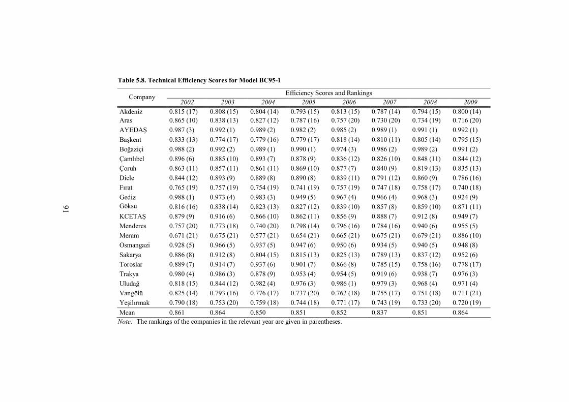
91


Efficiency Scores and Rankings Company 2002 2003 2004 2005 2006 2007 2008 2009

Akdeniz 0.815 (17) 0.808 (15) 0.804 (14) 0.793 (15) 0.813 (15) 0.787 (14) 0.794 (15) 0.800 (14) Aras 0.865 (10) 0.838 (13) 0.827 (12) 0.787 (16) 0.757 (20) 0.730 (20) 0.734 (19) 0.716 (20) AYEDAŞ 0.987 (3) 0.992 (1) 0.989 (2) 0.982 (2) 0.985 (2) 0.989 (1) 0.991 (1) 0.992 (1) Başkent 0.833 (13) 0.774 (17) 0.779 (16) 0.779 (17) 0.818 (14) 0.810 (11) 0.805 (14) 0.795 (15) Boğaziçi 0.988 (2) 0.992 (2) 0.989 (1) 0.990 (1) 0.974 (3) 0.986 (2) 0.989 (2) 0.991 (2) Çamlıbel 0.896 (6) 0.885 (10) 0.893 (7) 0.878 (9) 0.836 (12) 0.826 (10) 0.848 (11) 0.844 (12) Çoruh 0.863 (11) 0.857 (11) 0.861 (11) 0.869 (10) 0.877 (7) 0.840 (9) 0.819 (13) 0.835 (13) Dicle 0.844 (12) 0.893 (9) 0.889 (8) 0.890 (8) 0.839 (11) 0.791 (12) 0.860 (9) 0.786 (16) Fırat 0.765 (19) 0.757 (19) 0.754 (19) 0.741 (19) 0.757 (19) 0.747 (18) 0.758 (17) 0.740 (18) Gediz 0.988 (1) 0.973 (4) 0.983 (3) 0.949 (5) 0.967 (4) 0.966 (4) 0.968 (3) 0.924 (9) Göksu 0.816 (16) 0.838 (14) 0.823 (13) 0.827 (12) 0.839 (10) 0.857 (8) 0.859 (10) 0.871 (11) KCETAŞ 0.879 (9) 0.916 (6) 0.866 (10) 0.862 (11) 0.856 (9) 0.888 (7) 0.912 (8) 0.949 (7) Menderes 0.757 (20) 0.773 (18) 0.740 (20) 0.798 (14) 0.796 (16) 0.784 (16) 0.940 (6) 0.955 (5) Meram 0.671 (21) 0.675 (21) 0.577 (21) 0.654 (21) 0.665 (21) 0.675 (21) 0.679 (21) 0.886 (10) Osmangazi 0.928 (5) 0.966 (5) 0.937 (5) 0.947 (6) 0.950 (6) 0.934 (5) 0.940 (5) 0.948 (8) Sakarya 0.886 (8) 0.912 (8) 0.804 (15) 0.815 (13) 0.825 (13) 0.789 (13) 0.837 (12) 0.952 (6) Toroslar 0.889 (7) 0.914 (7) 0.937 (6) 0.901 (7) 0.866 (8) 0.785 (15) 0.758 (16) 0.778 (17) Trakya 0.980 (4) 0.986 (3) 0.878 (9) 0.953 (4) 0.954 (5) 0.919 (6) 0.938 (7) 0.976 (3) Uludağ 0.818 (15) 0.844 (12) 0.982 (4) 0.976 (3) 0.986 (1) 0.979 (3) 0.968 (4) 0.971 (4) Vangölü 0.825 (14) 0.793 (16) 0.776 (17) 0.737 (20) 0.762 (18) 0.755 (17) 0.751 (18) 0.711 (21) Yeşilırmak 0.790 (18) 0.753 (20) 0.759 (18) 0.744 (18) 0.771 (17) 0.743 (19) 0.733 (20) 0.720 (19) Mean 0.861 0.864 0.850 0.851 0.852 0.837 0.851 0.864

Note: The rankings of the companies in the relevant year are given in parentheses.

91

92





92

93





93

94

Table 5.11. Average Efficiency Scores for Alternative BC95 Models

Average Efficiency Scores Company BC95-1 BC95-2 BC95-3

Akdeniz 0.802 0.826 0.786 Aras 0.782 0.885 0.856 AYEDAŞ 0.988 0.987 0.987 Başkent 0.799 0.813 0.807 Boğaziçi 0.987 0.985 0.984 Çamlıbel 0.863 0.934 0.898 Çoruh 0.853 0.954 0.928 Dicle 0.849 0.884 0.842 Fırat 0.752 0.820 0.777 Gediz 0.965 0.955 0.955 Göksu 0.841 0.831 0.783 KCETAŞ 0.891 0.911 0.880 Menderes 0.818 0.832 0.796 Meram 0.685 0.682 0.664 Osmangazi 0.944 0.933 0.917 Sakarya 0.852 0.836 0.819 Toroslar 0.853 0.882 0.865 Trakya 0.948 0.934 0.930 Uludağ 0.940 0.935 0.935 Vangölü 0.764 0.855 0.770 Yeşilırmak 0.752 0.878 0.823 Table 5.12 presents summary statistics of efficiency scores obtained using

alternative BC95 models. Looking into these statistics, one may claim that these

models produced rather similar efficiency levels. The average of the efficiency

scores is about 0.86, and the scores range between 0.55 and 0.99. As stated before,

a more comprehensive comparison between all alternative models applied in this

study will be made in the following section.

Table 5.12. Summary Statistics of Technical Efficiency Scores for Alternative BC95 Models

Summary Statistics Model Mean Minimum Maximum Median Std. Dev.

BC95-1 0.854 0.577

0.992

0.778 0.092 BC95-2 0.883 0.55 0.993 0.85 0.083

BC95-3 0.857 0.546 0.995 0.804 0.094

95

5.3. COMPARISON BETWEEN ALTERNATIVE BC92&BC95 MODELS

Before comparing the efficiency and rank estimations of the alternative models,

we firstly looked at the parameter estimates of different distance functions given

in Table 5.1 and Table 5.7.

First of all, it has been noticed that BC92&BC95 models produced rather different

estimated values for first-order output coefficients. However, there exists a

consistency between all alternative models in terms of scale of return in the

market. To be more precise, in all alternative models sum of the first-order output

coefficients has been found less than 1 in absolute value, indicating that the

presence of increasing returns to scale is witnessed by all models.

The magnitude of the first-order input parameters obtained using BC92&BC95

models are not similar to each other. Among the inputs considered, distribution

line has been determined as the most important input by BC92 models, while

BC95 models indicates transformers as the most crucial input. However, all BC95

models reached a consistent result with regard to the quality variable: The

coefficient of the quality variable is found to be statistically insignificant, meaning

that taking the quality into account does not alter the efficiency score estimations

drastically.

All alternative BC92&BC95 models estimate a positive coefficient for the time

trend which is included into distance functions to explain the shift in the

production function. The finding of a positive coefficient for the time trend means

that the input isoquant curve has been shifting to left-down over time. In other

words, the market has been advancing technologically. However, this coefficient

has been found to be slightly insignificant in BC95 models, while it is significant

in BC92-3 model.

96

Alternative BC92&BC95 models exhibit a consistency regarding the structure of

error variance. Accordingly, it has been shown that the coefficient of variance

ratio is statistically significant and rather close to 1, indicating the importance

of inefficiency effects rather than random error effects in this study.

When comparing the technical efficiency scores obtained in BC92&BC95 models,

we firstly realize that the estimated efficiency scores are substantially higher in

BC95 models than those in BC92 models. This difference may be seen clearly

from Table 5.6 and Table 5.12: The average efficiency score in BC95 models is

about 0.86 while it is approximately 0.64 in BC92 models. The minimum levels of

efficiency estimations are especially lower in BC92 models compared to those of

BC95 models.

In addition to comparison of average efficiency estimations resulted from

different models, it is also possible to compare efficiency estimations of these

models for each company at each time period. This is achieved by calculating the

correlations between efficiency estimations of different models, which is

presented in Table 5.13. Making firstly a comparison between the same kinds of

models, we observe rather strong correlations between them: The correlations

between efficiency estimations of BC92 models range from 0.989 to 0.995. As for

the efficiency estimations of BC95 models, their correlations with each other

reduce slightly, but still taking rather high values between 0.870 and 0.962. When

making comparisons between efficiency estimations of BC92&BC95 models, we

continue to observe rather high correlations between BC92 models and Model

BC95-1, ranging between 0.709 and 0.751. However, the same conclusion cannot

be drawn with respect to the remaining BC95 models. Their correlations with

BC92 models drop substantially to the levels between 0.494 and 0.574. Indeed,

the reasons for the finding of relatively low correlations between efficiency

estimations of BC92&BC95 models are indeed apparent to us. Firstly, these two

models are rather different structurally in the sense that in contrast to BC92, BC95

97

includes environmental variables which may affect the efficiency estimations.

Secondly and most importantly, these environmental variables we included into

BC95 models are generally found to be statistically significant, meaning that they

change the efficiency estimations drastically.

Table 5.13. Correlations of Technical Efficiency Scores Using Alternative Models

Correlations

BC92-1 BC9-22 BC92-3 BC95-1 BC95-2 BC95-3 BC92-1 1.000 0.995 0.989 0.709 0.494 0.533 BC92-2 1.000 0.991 0.714 0.510 0.549 BC92-3 1.000 0.751 0.514 0.574 BC95-1 1.000 0.870 0.920 BC95-2 1.000 0.962 BC95-3 1.000 We also compared the ranking estimations of alternative models via correlations

which are tabulated in Table 5.14. We observe that the pattern of the correlations

between ranking estimations is very similar to that of correlations between

efficiency estimations.

Table 5.14. Correlations of Rankings Using Alternative Models

Correlations

BC92-1 BC9-22 BC92-3 BC95-1 BC95-2 BC95-3 BC92-1 1.000 0.992 0.978 0.729 0.510 0.550 BC92-2 1.000 0.986 0.732 0.522 0.567 BC92-3 1.000 0.773 0.529 0.593 BC95-1 1.000 0.849 0.899 BC95-2 1.000 0.949 BC95-3 1.000

98

CHAPTER 6

CONCLUSION & FURTHER STUDIES

In this study, technical efficiencies of Turkish electricity distribution companies

have been analyzed for the period between 2002 and 2009. For this aim, we used

SFA method, which is based on an input distance function. In order to see whether

the efficiency scores of the companies are sensitive to the model specifications,

we preferred to utilize two different SFA models (BC92&BC95), and also

generate three different versions for each model by adding a new input or

environmental variable into previous version of a given model.

First of all, it has been shown that all alternative specifications of both models

(BC92&BC95) satisfy the regularity conditions. In other words, the first-order

coefficients of the outputs and inputs are found to be negative and positive,

respectively. Examining the first-order coefficients of the outputs, we see that

these coefficients are statistically significant in all alternative model

specifications, although their magnitude may change depending on the model

which we utilized. All model specifications, however, tell the same story

regarding the returns to scale in Turkish electricity distribution market: The sum

of the first-order coefficients of outputs are found to be less than one in all model

specifications, indicating the presence of increasing returns to scale at the mean of

the data. This finding is line with that of Bağdadioğlu and Weyman-Jones (2008),

but contrary to that of Bağdadioğlu and Senyücel (2010).

Looking into the estimated first-order input coefficients, we saw that these

coefficients take the positive values as expected in all alternative model

specifications. In addition, all first-order input coefficients – except that of

“quality of electricity delivered” are found to be statistically significant in all

99

model specifications. This finding suggests that the three inputs considered in this

study (number of employees, lengthy of the distribution line and transformer

capacity) are of importance in enhancing the technical efficiency of the electricity

distribution companies. Among them, the most crucial input varies depending on

the model specifications: According to the models based on BC92, the distribution

lines is critical for electricity distribution companies to enhance their efficiencies.

The models based on BC92, on the other hand, indicates the transformers as the

most important input significantly affecting efficiency.

Our finding that the coefficient of quality of electricity delivered is not

statistically significant deserves some further exploration because of the fact that

it may seem to be interesting and somewhat unexpected at first glance. In adding

the quality variable into model specifications, we aimed to observe whether the

measured inefficiency of an individual distribution company is due to poor

employment of the other inputs or due to higher input requirements as a result of a

higher quality level. The insignificancy of this input variable means that the

inclusion of the quality variable into models does not affect estimated efficiency

scores of the electricity distribution companies. In other words, in our case, the

reason for the inefficiency of a distribution company with a higher quality level is

not higher input requirements needed to achieve this high quality level. Instead,

the reason is the poor employment of the other inputs, namely just itself of the

technical inefficiency. Meanwhile, in the literature, there exist studies reaching

conflicting conclusions regarding the importance of the quality variable in the

efficiency analysis. For example, Coelli et al. (2008) also showed that the

incorporation of the quality does not affect significantly the technical efficiency

scores. On the other hand, several studies such as Growitsch et al. (2009),

Giannakis et al. (2005) and Bağdadioğlu and Senyücel (2010) revealed the

importance and significance of the quality variable in the efficiency analysis.

However, it should be noticed that Growitsch et al. (2009) and Bağdadioğlu and

Senyücel (2010) found that the inclusion of the quality variable reduces estimated

100

efficiency scores, which is completely in contrast to the finding of Giannakis et al.

(2005).

We included a time trend into all input distance functions to catch the changes in

the efficiencies due to any shift in the production function. All alternative

BC92&BC95 models estimated a positive coefficient for the time trend, indicating

the presence of a technological progress in the electricity distribution market over

time. However, this coefficient has been found to be slightly insignificant in BC95

models, while it is significant in BC92 models. Despite, given that both

magnitudes of this coefficient and its t-ratios are generally rather high in BC95

models, it can be concluded that our models witnessed a mild technological

progress (approximately 0.6%-0.8% per year) in the electricity distribution market

over time.

With regard to the underlying error variance, our study reached to a rather

consistent conclusion: In all alternative BC92&BC95 models, the coefficient of

variance ratio ( ) is found to be statistically significant and rather close to one,

indicating the importance of inefficiency effects rather than random error effects

in this study. This conclusion is in line with those of previous studies such as

Bağdadioğlu and Weyman-Jones (2008) and Bağdadioğlu and Senyücel (2010).

According to this finding, the random error effects are of little importance in

Turkish electricity distribution market, thus one may claim that instead of SFA the

deterministic methods such as DEA and COLS can be safely used in the

efficiency analysis of this market.

BC95 models include three environmental variables which have potential to affect

the inefficiency of electricity distribution companies. The first environmental

factor is the customer density of the regions, measured in terms of number of

customers per km of distribution line. This study revealed that the customer

density of a region positively affects the technical efficiency of the relevant

101

distribution company, which is not a surprising result given that companies

operating in crowded regions have a natural efficiency advantage over those with

a weak customer density.

Another environmental factor considered is the customer structure defined as

proportion of sales in MWh to residential customers to total sales. We find that

efficiencies of the companies serving to mostly the residential customers are

higher than those of other companies. This conclusion is line with that of

Hirschhausen et al. (2006). However, the reason behind this finding is not

apparent to us at the moment, thus it deserves some further analysis.

As another environmental variable, we also take into account a time trend. The

results revealed that the efficiencies of the distribution companies decline over

time, but in a statistically insignificant extent.

As for the efficiency estimations of the alternative models, the main conclusion

revealed by our study is that efficiency estimations of the BC95 models are

notably higher than those of the BC92 models: The average efficiency score in

BC95 models is about 0.86 while it is approximately 0.64 in BC92 models. Given

that the most important difference between BC92&BC95 models is the

environmental variables included into the the BC95 models, we may argue that

the efficiency estimation differences between BC92&BC95 models can be

attributed to these environmental variables. In other words, an important part of

the technical inefficiency of the electricity distribution companies may be due to

the environmental variables such as customer density and structure of the regions

in which the distribution companies operate. One should notice that the

distribution companies have very limited capability to control these environmental

variables. Overall, we may conclude that this study witnessed the importance of

the environmental variables in the efficiency studies regarding Turkish electricity

distribution market.

102

In searching the consistency between alternative models, we also compared the

technical efficiency estimations of these models by calculating correlations. The

results show that regarding both efficiency scores and ranking there exist strong

correlations between estimations of the models based on the same model type

(BC92 or BC95). On the other hand, comparing estimations of the models based

on the different model type, the correlations dropped to the level of 0.494.

Looking at the most efficient and inefficient companies estimated by alternative

models, we observe that Trakya, AYEDAŞ, KCETAŞ and Osmangazi appear as

the most efficient companies, and on the side of inefficient companies, Başkent,

Yeşilırmak and Toroslar line up, according to BC92 models. As for the BC95

models, the efficiency scores and rankings of the companies change over time.

However, generally speaking, one may conclude that AYEDAŞ, Boğaziçi and

Gediz are the companies operating most efficiently, while Meram, Fırat and

Vangölü are the worst performers. The main conclusion obtained from these

comparisons is that the efficiency and ranking estimations have been rather

sensitive to the models used. Thus, it appears to be of crucial importance to work

on different model specifications in the efficiency studies.

Another important conclusion drawn from this study is that in spite of efficiency

differences between estimations of the alternative models, at the very beginning of

the liberalization of electricity distribution market there appear considerable

opportunities of improvement in the efficiencies. For example, the most

inefficient companies such as Yeşilırmak, Meram, Fırat and Toroslar could

achieve almost the same output levels even by reducing the inputs by half.

However, decreasing the inputs does not seem to be an appropriate strategy in

enhancing the efficiency of the Turkish electricity distribution market. For

example, although, as seen from the graphs presented in Appendix A, Başkent and

Meram reduced the number of employees substantially following their

privatizations, these reorganizations have not enhanced their efficiency

103

performances. In addition, given that the electricity usage in Turkey have been in

an increasing trend and this trend will continue in the coming years, we may

expect that the efficiency of the distribution companies may increase without any

need to cut in input usage.

It may be possible to extend this study in several directions: First of all, the

loss/theft ratios, which are very high especially in the eastern part of Turkey, may

be taken into account. We preferred not to do it for two reasons: Firstly, we

measured the technical efficiencies by using physical quantities of inputs, not their

costs. Secondly, the electricity distribution companies achieve to reach the

electricity to end-users, but mostly fail in metering the electricity usage and

collecting the bills in the eastern part of Turkey. Thus, taking directly into

consideration the loss/theft differences would lead to substantial and unfair drops

in the efficiency estimations of the companies operated in the eastern part of

Turkey. This is exactly what Bağdadioğlu and Senyücel (2010) reported. They

estimated 0.50 and 0.47 as efficiencies of Dicle and Vangölü, respectively when

ignoring the loss/theft differences. Taking into account the loss/theft differences,

the efficiencies of these two companies dropped to 0.10 and 0.12 respectively,

which seem to be incredibly low.

Since the electricity distribution companies have been started to be handed over to

private sector very recently, in this study we could not examine effects of the

change in the ownerships on the efficiency of the companies. For the coming

years, it would be of great interest to work on this issue.

In literature there are plenty of studies comparing the efficiency estimations

obtained from parametric and non-parametric methods. To the best of our

knowledge, there is no such a study estimating simultaneously the efficiency

levels of Turkish electricity distribution companies with both parametric and non-

parametric methods. This may be another topic for a future work. However, one

104

should not expect a strong consistency between estimations of these parametric

and non-parametric methods, given that the results of the previous studies in the

literature have been mostly in this direction.

The cost related with the distribution of electricity is 11% of the total electricity

tariff. The most important cost item in the electricity tariffs is the generation cost

with a share of 64%. Thus, efficiency enhancements in the electricity generation

are as important as those relevant in the electricity distribution. In literature, to the

best of our knowledge, only Sarıca and Or (2007) analyzed the efficiency

performances of 65 thermal, hydro and wind electricity power plants using DEA.

Thus, one area of future work may be studying on efficiencies of electricity

generation plants, especially via SFA.

105

REFERENCES

Aigner, D.J., and Chu, S.F. (1968), On Estimating the Industry Production Function, American Economic Review, 58(4), 826–39.

Aigner, D.J., Lovelly, C.A.K. , and Schmidt, P.J. (1977), Formulation and Estimation of Stochastic Frontier Production Function Models, Journal of Econometrics, 6.

Appa G., Costa, C.A.B., Chagas, M.P., Ferreira, F.C., and Soares, J.O. (2010), DEA in X-factor evaluation fort he Brazilian Electricity Distribution Industry, London School of Economics, Working Papers, LSEOR 10.121.

Atiyas, İ, and Dutz, M. (2004), Competition and Regulatory Reform in the Turkish Electricity Industry, Final Version Published in B.M Hoekman and S. Togan (eds.) Turkey: Economic Reforms and Accession to the European Union, Washington, DC: The World Bank and the CEPR, 2005.

Bağdadioğlu, N. (1996), Privatisation, Ownership and Technical Efficiency in the Turkish Electricity Supply Industry, Pacific and Asian Journal of Energy, 6, 25-37

Bağdadioğlu, N., Price, C.M.W., Weyman-Jones, T.G. (1996), Efficiency and Ownership in Electricity Distribution: A Non-parametric Model of the Turkish Experience. Energy Economics 18, 1–23.

Bağdadioğlu, N. (2005), The Efficiency Consequences of Resisting Changes in a Changing World: Evidence from the Turkish Electricity Distribution, International Journal of Business, Management and Economics, 1, 2, 23–44.

Bağdadioğlu, N., Waddams Price, C., and Weyman-Jones, T. (2007), Measuring Potential Gains from Mergers among Electricity Distribution Companies in Turkey Using a Non-parametric Model, The Energy Journal, 28(2), 83-100.

Bağdadioğlu, N., and Weyman-Jones, T. (2008), Panel Data Stochastic Frontier Analysis for Energy Network Regulation, Draft Version, www.cepe.ethz.ch/workshop2008/Weyman-Jones, last visited on January 2011.

Bağdadioğlu, N. (2009), An Application of Incentive Regulation of Service Quality in the Turkish Electricity Distribution Sector, Gazi Üniversitesi İktisadi ve İdari Bilimler Fakültesi Dergisi, 11(1), (2009), 23-44 (in Turkish).

Bağdadioğlu, N, and Senyücel, O. (2010), Service Quality Regulation in Electricity Distribution, paper presented in 6th International Scientific Conference, May 13–14, 2010, Vilnius, Lithuania.

106

Bağdadioğlu, N., and Weyman-Jones, T. (2010), Stochastic Frontier Panel Data Modelling for Regulatory Bechmarking: An Application to the Turkish Electricity Distribution Sector, İktisat, İşletme ve Finans, 25(297), 97-119

Banker, R.D., Charnes, A., and Cooper, W.W. (1984), Some Models for Estimating Technical and Scale Inefficiencies in Data Envelopment Analysis, Management Science, 30(9), 1078 – 1092.

Banker, R.D., Gadh, V.M., and Gorr, W.L. (1993), A Monte Carlo Comparison of Two Production Frontier Estimation Methods: Corrected Ordinary Least Squares and Data Envelopment Analysis, European Journal of Operational Research, 67, 332-343.

Battese, G.E., and Corra, G. (1977) Estimation of a Production Frontier Model with Application to the Pastoral Zone of Easter Australia, Australian Journal of Agricultural Economics, 21(3): 167–179.

Battese, G.E. and Coelli, T.J. (1992), Frontier Production Function, Technical Efficiency and Panel Data: With Application to Paddy Farmers in India. Journal of Productivity Analysis, 3, 153-169.

Battese, G.E., and Coelli, T.J. (1995), A Model for Technical Inefficiency Effects in a Stochastic Frontier Production Function for Panel Data, Empirical Economics, 20, 325-332.

Boles, J. N. (1966), Efficiency Squared – Efficient Computation of Efficiency Indexes, Proceedings of Thirty Ninth Annual Meeting of the Western Farm Economics Association, 137-42.

Charnes, A., Cooper, W.W., and Rhodes, E. (1978), Measuring the Efficiency of Decision Making Units, European Journal of Operational Research, 429-444.

Coelli, T. (1996), A Guide to FRONTIER Version 4.1: A Computer Program for Frontier Production Function Estimation, CEPA Working Paper 96/07, Department of Econometrics, University of New England, Armidale, Australia.

Coelli, T., and Perlman., S. (2000), Technical Efficiency of European Railways: A Distance Function Approach, Applied Economics, 32.

Coelli, T.J., Rao, D.S.P., O’Donnell, C.J., and Battese, G.E. (2005), An Introduction to Efficiency and Productivity Analysis, 2nd edition, Springer

Coelli, T. J., Crespo, H., Paszukiewicz, A., Perelma, S., Plagnet, M.A., and Romano, E. (2008), Incorporating Quality of Service in a Benchmarking Model: An Application to French Electricity Distribution Operators, www.cepe.ethz.ch/workshop2008/Plagnet, last visited on January 2011

107

Emrouznejad, A., Parker, B.R., and Tavares, G. (2008), Evaluation of Research in Efficiency and Productivity: A Survey and Analysis of the First 30 Years of Scholarly Literature in DEA, Socio-Economic Planning Sciences, 42 (3), 151-157.

Erdoğdu (2009), Some Thoughts on the Turkish Electricity Distribution Industry, Renewable and Sustainable Energy Reviews, 13, 1485–1494.

Fare, R., Grosskopf, S., and Logan, J. (1983), The Relative Efficiency of Illinois Electric Utilities, Resources and Energy 5, 349-367.

Fare, R., and Primont, D. (1995), Multi-Output Production and Duality: Theory and Applications, Boston, Kluwer Academic Publishers.

Farrell, M.J. (1957), The Measurement of Productive Efficiency, Journal of Royal Statistical Society, Series A, General. 120, 253-281.

Giannakis, D., Jamasb, T. and Pollitt, M. (2005), Benchmarking and Incentive Regulation of Quality of Service: An Application to the UK Electricity Distribution Networks, Energy Policy 33(17), 2256–2271.

Greene, W.M. (1993), The Econometric Approach to Efficiency Analysis, The Measurement of Productive Efficiency: Techniques and Applications, Published in Harold O. Fried, Lovell, C.A.K. and Schmidt, S.S. (eds.), Oxford University Press: 68–119.

Growitsch, C., Jamasb, T., and Pollitt, M. (2009), Quality of Service, Efficiency, and Scale in Network Industries: An Analysis of European Electricity Distribution, Applied Economics 41(20), 2555–2570.

Hakman, S. (2009), Rising Power Demand in Turkey – Utlizing Renewable Resources, www.energy2020.at/download2009/slides/energy2020_hakman.pdf, last visited on January 2011

Hattori, T., Jamasb, T., and Pollitt, M. (2005), Electricity Distribution in the UK and Japan: A Comparative Efficiency Analysis 1985-1998, Energy Journal, 26 (2): 23-47.

Hirschhausen, C. von, Cullman, A., and Kappeler, A. (2006), Efficiency Analysis of German Electricity Distribution Utilities: Nonparametric and Parametric Tests, Applied Economics, 38, 2553-2566.

Jacobs, R. (2000), Alternative Methods to Examine Hospital Efficiency: Data Envelopment Analysis and Stochastic Frontier Analysis, University of York, Centre for Health Economics (CHE) Discussion Paper no. 177.

108

Jamasb, T., Pollitt, M. (2001), Benchmarking and Regulation of Electricity Transmission and Distribution Utilities: Lessons from International Experience. Department of Applied Economics, University of Cambridge.

Judge, G., Griffiths, W.E., Hill, R.C., Lutkepohl, H., and Lee, T.C. (1985), The Theory and Practice and Econometrics, New York, John Wiley.

Koopmans, T.C. (1951), An Analysis of Production as an Efficient Combination of Activities” in T.C. Koopmans ed. Activity Analysis of production and Allocation, Cawles Commission for Research in Economics, 13, New York.

Kumbhakar, S.C. (1990), Production Frontiers, Panel Data, and Time-Varying Technical İnefficiency, Journal of Econometrics, 46(1-2), 201-211

Kumbhakar, S.C., Lovell, C.A.K. (2000) Stochastic Frontier Analysis, Cambridge University Press, Cambridge.

Lovell, C.A.K., Richardson, S., Travers, P., and Wood, L. (1994), Resources and Functionings: A New View of Inequality in Australia, in W.Eichhorn (ed.), Models and Measurement of Welfare and Inequality, Springer-Verlag, Heidelberg, 1994.

Meeusen, W., and Van den Broeck, J. (1977), Efficiency Estimation from Cobb-Douglas Production Functions with Composed Error. International Economic Review, 18: 435–444.

Mert, Y.K. (2010), Privatization and Liberalization of the Electricity Sector in Turkey, www.ecoprivatization.org/Libraries/Other_Publications/Privatization_and_Liberalization_of_the_Electricity_Sector_in_Turkey.sflb.ashx, last visited on January 2011

Mortimer, D. (2002), Competing Methods for Efficiency Measurement A Systematic Review of Direct DEA vs SFA/DFA Comparisons, Research Associate, School of Medicine, Health Policy & Practice, University of East Anglia, Working Paper no. 136.

Neuberg, L. (1977), Two Issues in Municipal Ownership of Electric Power Distribution Systems, Bell Journal of Economics, 8, 303-323.

Odyakmaz, N. (2009), The Comparative Performance Analysis of Turkish Electricity Distribution Companies in the Framework of Performance-based Regulation, Unpublished Phd Thesis, Department of Economics, Hacettepe University, Ankara (in Turkish).

ÖİB (2010), Privatization of Turkey’s Electricity Distribution Industry, Teaser, Özelleştirme İdaresi Başkanlığı.

109

Rasmussen, S. (2010), Scale Efficiency in Danish Agriculture: An Input Distance–Function Approach, European Review of Agricultural Economics, 37, 3, 335–367

Ray, S.C. (2004), Data Envelopment Analysis: Theory and Techniques for Economics and Operations Research, New York, Cambridge University Press.

Ritter, C., and Simar, L. (1997) Pitfalls of Normal-Gamma Stochastic Frontier Models Journal of Productivity Analysis, 8: 167–182.

Rungsuriyawiboon, S., and Coelli, T. (2004), Regulatory Reform and Economic Performance in US Electricity Generation, Working Paper 06/2004, CEPA Working Papers Series, University of Queensland, School of Economics.

Sarıca, K., and Or, İ. (2007), Efficiency Assessment of Turkish Power Plants Using Data Envelopment Analysis, Energy, 32 (8): 1484-1499.

Shephard, R.W. (1953), Cost and Production Functions, Princeton University Press.

Shephard, R.W. (1970), The Theory of Cost and Production Functions, Princeton University Press.

Simar, L., and Wilson, P.W. (2000), A General Methodology for Bootstrapping in Non-parametric Frontier Models, Journal of Applied Statistics 27, 779-802.

Söderberg M. (2007), An Exploration of Factors Influencing Cost Inefficiency in Swedish Electricity Distribution using Stochastic Frontier Analysis, University of South Australia

Starodubtsew, I. (2007), Reform of The Turkish Electrical Energy Sector: Basic Principles and Interim Results, The Centre for Energy, Petroleum and Mineral Law and Policy, The University of Dundee.

Stevenson, R.E. (1980), Likelihood Function for Generalized Stochastic Frontier Estimation, Journal of Econometrics, 13, 57-66.

110

APPENDIX A

GRAPHS OF VARIABLES 10

0000

022

0000

00

2002 2005 2009

Akdeniz

1000

000

2200

0000

2002 2005 2009

Aras

1000

000

2200

0000

2002 2005 2009

AYEDAŞ

1000

000

2200

0000

2002 2005 2009

Başkent10

0000

022

0000

00

2002 2005 2009

Boğaziçi

1000

000

2200

0000

2002 2005 2009

Çamlıbel

1000

000

2200

0000

2002 2005 2009

Çoruh

1000

000

2200

0000

2002 2005 2009

Dicle

1000

000

2200

0000

2002 2005 2009

Fırat

1000

000

2200

0000

2002 2005 2009

Gediz

1000

000

2200

0000

2002 2005 2009

Göksu

1000

000

2200

0000

2002 2005 2009

KCEDAŞ

1000

000

2200

0000

2002 2005 2009

Menderes

1000

000

2200

0000

2002 2005 2009

Meram

1000

000

2200

0000

2002 2005 2009

Osmangazi

1000

000

2200

0000

2002 2005 2009

Sakarya

1000

000

2200

0000

2002 2005 2009

Toroslar

1000

000

2200

0000

2002 2005 2009

Trakya

1000

000

2200

0000

2002 2005 2009

Uludağ

1000

000

2200

0000

2002 2005 2009

Vangölü

1000

000

2200

0000

2002 2005 2009

Yeşilırmak

elec

trici

ty d

eliv

ered

(MW

h)

years

Figure A.1. Electricity Delivered

111

3000

0040

0000

0

2002 2005 2009

Akdeniz

3000

0040

0000

0

2002 2005 2009

Aras

3000

0040

0000

0

2002 2005 2009

AYEDAŞ

3000

0040

0000

0

2002 2005 2009

Başkent

3000

0040

0000

02002 2005 2009

Boğaziçi

3000

0040

0000

0

2002 2005 2009

Çamlıbel

3000

0040

0000

0

2002 2005 2009

Çoruh

3000

0040

0000

0

2002 2005 2009

Dicle

3000

0040

0000

0

2002 2005 2009

Fırat

3000

0040

0000

0

2002 2005 2009

Gediz

3000

0040

0000

0

2002 2005 2009

Göksu

3000

0040

0000

0

2002 2005 2009

KCEDAŞ

3000

0040

0000

0

2002 2005 2009

Menderes

3000

0040

0000

0

2002 2005 2009

Meram

3000

0040

0000

0

2002 2005 2009

Osmangazi

3000

0040

0000

0

2002 2005 2009

Sakarya

3000

0040

0000

0

2002 2005 2009

Toroslar

3000

0040

0000

0

2002 2005 2009

Trakya

3000

0040

0000

0

2002 2005 2009

Uludağ

3000

0040

0000

0

2002 2005 2009

Vangölü

3000

0040

0000

0

2002 2005 2009

Yeşilırmak

num

ber o

f cus

tom

ers

years

Figure A.2. Number of Customers

112

500

4000

2002 2005 2009

Akdeniz

500

4000

2002 2005 2009

Aras

500

4000

2002 2005 2009

AYEDAŞ

500

4000

2002 2005 2009

Başkent

500

4000

2002 2005 2009

Boğaziçi

500

4000

2002 2005 2009

Çamlıbel

500

4000

2002 2005 2009

Çoruh

500

4000

2002 2005 2009

Dicle

500

4000

2002 2005 2009

Fırat

500

4000

2002 2005 2009

Gediz

500

4000

2002 2005 2009

Göksu

500

4000

2002 2005 2009

KCEDAŞ

500

4000

2002 2005 2009

Menderes

500

4000

2002 2005 2009

Meram

500

4000

2002 2005 2009

Osmangazi

500

4000

2002 2005 2009

Sakarya

500

4000

2002 2005 2009

Toroslar

500

4000

2002 2005 2009

Trakya

500

4000

2002 2005 2009

Uludağ

500

4000

2002 2005 2009

Vangölü

500

4000

2002 2005 2009

Yeşilırmak

num

ber o

f em

ploy

ees

years

Figure A.3. Number of Employees

113

1300

095

000

2002 2005 2009

Akdeniz

1300

095

000

2002 2005 2009

Aras

1300

095

000

2002 2005 2009

AYEDAŞ

1300

095

000

2002 2005 2009

Başkent

1300

095

000

2002 2005 2009

Boğaziçi

1300

095

000

2002 2005 2009

Çamlıbel

1300

095

000

2002 2005 2009

Çoruh

1300

095

000

2002 2005 2009

Dicle

1300

095

000

2002 2005 2009

Fırat

1300

095

000

2002 2005 2009

Gediz

1300

095

000

2002 2005 2009

Göksu

1300

095

000

2002 2005 2009

KCEDAŞ

1300

095

000

2002 2005 2009

Menderes

1300

095

000

2002 2005 2009

Meram

1300

095

000

2002 2005 2009

Osmangazi

1300

095

000

2002 2005 2009

Sakarya

1300

095

000

2002 2005 2009

Toroslar

1300

095

000

2002 2005 2009

Trakya

1300

095

000

2002 2005 2009

Uludağ

1300

095

000

2002 2005 2009

Vangölü

1300

095

000

2002 2005 2009

Yeşilırmak

leng

th o

f dis

tribu

tion

line

(km

)

years

Figure A.4. Length of Distribution Line

114

900

1300

0

2002 2005 2009

Akdeniz

900

1300

0

2002 2005 2009

Aras

900

1300

0

2002 2005 2009

AYEDAŞ

900

1300

0

2002 2005 2009

Başkent

900

1300

0

2002 2005 2009

Boğaziçi

900

1300

0

2002 2005 2009

Çamlıbel

900

1300

0

2002 2005 2009

Çoruh90

013

000

2002 2005 2009

Dicle

900

1300

0

2002 2005 2009

Fırat

900

1300

0

2002 2005 2009

Gediz

900

1300

0

2002 2005 2009

Göksu

900

1300

0

2002 2005 2009

KCEDAŞ

900

1300

0

2002 2005 2009

Menderes

900

1300

0

2002 2005 2009

Meram

900

1300

0

2002 2005 2009

Osmangazi

900

1300

0

2002 2005 2009

Sakarya

900

1300

0

2002 2005 2009

Toroslar

900

1300

0

2002 2005 2009

Trakya

900

1300

0

2002 2005 2009

Uludağ

900

1300

0

2002 2005 2009

Vangölü

900

1300

0

2002 2005 2009

Yeşilırmak

trans

form

er c

apac

ity (M

VA)

years

Figure A.5. Transformer Capacity

115

.002

.2

2002 2005 2009

Akdeniz

.002

.2

2002 2005 2009

Aras

.002

.2

2002 2005 2009

AYEDAŞ

.002

.2

2002 2005 2009

Başkent

.002

.2

2002 2005 2009

Boğaziçi

.002

.2

2002 2005 2009

Çamlıbel

.002

.2

2002 2005 2009

Çoruh.0

02.2

2002 2005 2009

Dicle

.002

.2

2002 2005 2009

Fırat

.002

.2

2002 2005 2009

Gediz

.002

.2

2002 2005 2009

Göksu

.002

.2

2002 2005 2009

KCEDAŞ

.002

.2

2002 2005 2009

Menderes

.002

.2

2002 2005 2009

Meram

.002

.2

2002 2005 2009

Osmangazi

.002

.2

2002 2005 2009

Sakarya

.002

.2

2002 2005 2009

Toroslar

.002

.2

2002 2005 2009

Trakya

.002

.2

2002 2005 2009

Uludağ

.002

.2

2002 2005 2009

Vangölü

.002

.2

2002 2005 2009

Yeşilırmak

outa

ge h

ours

per

cus

tom

er

years

Figure A.6. Outage Hours per Customer

116

1513

0

2002 2005 2009

Akdeniz

1513

0

2002 2005 2009

Aras

1513

0

2002 2005 2009

AYEDAŞ

1513

0

2002 2005 2009

Başkent

1513

0

2002 2005 2009

Boğaziçi

1513

0

2002 2005 2009

Çamlıbel

1513

0

2002 2005 2009

Çoruh15

130

2002 2005 2009

Dicle

1513

0

2002 2005 2009

Fırat

1513

0

2002 2005 2009

Gediz

1513

0

2002 2005 2009

Göksu

1513

0

2002 2005 2009

KCEDAŞ

1513

0

2002 2005 2009

Menderes

1513

0

2002 2005 2009

Meram

1513

0

2002 2005 2009

Osmangazi

1513

0

2002 2005 2009

Sakarya

1513

0

2002 2005 2009

Toroslar

1513

0

2002 2005 2009

Trakya

1513

0

2002 2005 2009

Uludağ

1513

0

2002 2005 2009

Vangölü

1513

0

2002 2005 2009

Yeşilırmak

cust

omer

den

sity

(cus

tom

er/k

m)

years

Figure A.7. Customer Density

117

1050

2002 2005 2009

Akdeniz

1050

2002 2005 2009

Aras

1050

2002 2005 2009

AYEDAŞ

1050

2002 2005 2009

Başkent

1050

2002 2005 2009

Boğaziçi

1050

2002 2005 2009

Çamlıbel

1050

2002 2005 2009

Çoruh10

50

2002 2005 2009

Dicle

1050

2002 2005 2009

Fırat

1050

2002 2005 2009

Gediz

1050

2002 2005 2009

Göksu

1050

2002 2005 2009

KCEDAŞ

1050

2002 2005 2009

Menderes

1050

2002 2005 2009

Meram

1050

2002 2005 2009

Osmangazi

1050

2002 2005 2009

Sakarya

1050

2002 2005 2009

Toroslar

1050

2002 2005 2009

Trakya

1050

2002 2005 2009

Uludağ

1050

2002 2005 2009

Vangölü

1050

2002 2005 2009

Yeşilırmak

cust

omer

stru

ctur

e (%

)

years

Figure A.8. Customer Structure

measuring the efficiency of the turkish electric distribution sector

Documents