mechanical and thermal sources in a micropolar generalized thermoelastic medium
TRANSCRIPT

Journal of Sound and <ibration (2001) 239(3), 467}488doi:10.1006/jsvi.2000.3143, available online at http://www.idealibrary.com on
MECHANICAL AND THERMAL SOURCESIN A MICROPOLAR GENERALIZED
THERMOELASTIC MEDIUM
R. KUMAR AND S. DESWAL
Department of Mathematics, Kurukshetra ;niversity, Kurukshetra 136 119, Haryana, India.E-mail: vidya.kuk.ernet.in
(Received 27 January 2000, and in ,nal form 9 June 2000)
The disturbance due to mechanical and thermal sources in a homogeneous, isotropic,micropolar generalized thermoelastic half-space is investigated by the use of Laplace}Fourier transform technique. The analytical expressions of displacement components,normal force stress, tangential force stress and temperature "eld so obtained have beeninverted by using a numerical technique. Numerical results are presented graphically fora magnesium crystal like material.
( 2001 Academic Press
1. INTRODUCTION
The linear theory of elasticity is of paramount importance in the stress analysis of steel,which is the most common engineering structural material. To a lesser extent linearelasticity describes the mechanical behaviour of other common solid materials, e.g.,concrete, wood and coal. However, this theory does not apply to the behaviour of many ofthe new synthetic materials of the elastomer and polymer type, e.g., polymethyl-methacrylate (perspex), polythylene, polyvinyl chloride.
Modern engineering structures are often made up of materials possessing an internalstructure. Polycrystalline materials, materials with "brous or coarse grain structure come inthis category. Classical elasticity is inadequate to represent the behaviour of such materials.The analysis of such materials requires incorporating the theory of oriented media.&&Micropolar elasticity'' termed by Eringen [1] is used to describe the deformation of elasticmedia with oriented particles. A micropolar continuum is a collection of interconnectedparticles in the form of small rigid bodies undergoing both translational and rotationalmotions. Typical examples of such materials are granular media and multimolecular bodies,whose microstructures act as an evident part in their macroscopic responses. The physicalnature of these materials needs an asymmetric description of deformation, while theories forclassical continua fail to accurately predict their physical and mechanical behaviour. Forthis reason, micropolar theories were developed by Eringen [1}3] for elastic solids, #uidsand further for non-local polar "elds and are now universally accepted.
The coupled theory of thermoelasticity has been extended by including the thermalrelaxation time in the constitutive equations by Lord and Shulman (L}S) [4] and Greenand Lindsay (G}L) [5]. These new theories eliminate the paradox of in"nite velocity of heatpropagation and are termed as generalized theories of thermoelasticity. In view of theexperimental evidence available in favour of "niteness of heat propagation speed,
0022-460X/01/030467#22 $35.00/0 ( 2001 Academic Press
468 R. KUMAR AND S. DESWAL
generalized thermoelasticity theories are supposed to be more realistic than theconventional theory in dealing with practical problems involving very large heat #uxesand/or short time intervals, like those occurring in laser units and energy channels.Recently, Green and Naghdi (G}N) [6}8] proposed a new generalized thermoelasticitytheory by including the &&thermal-displacement gradient'' among the constitutive variablesthat permit treatment of a much wider class of heat #ow problems. An important feature ofthis theory, which is not present in other thermoelasticity theories, is that this theory doesnot accommodate dissipation of thermal energy.
The linear theory of micropolar thermoelasticity was developed by extending the theoryof micropolar continua to include thermal e!ects by Eringen [9] and Nowacki [10].Di!erent authors [11}14] discussed di!erent problems in micropolar elasticity/micropolartheory of thermoelasticity.
The purpose of the present paper is to determine the normal displacement, normal forcestress, tangential couple stress and temperature distribution in a homogeneous, isotropic,micropolar generalized thermoelastic half-space due to instantaneous mechanical andthermal sources by applying integral transform techniques. Numerical techniques havebeen used to invert the integral transforms. The components of stresses, displacements andtemperature "eld are calculated for the mechanical and thermal impulses. Applications ofthe present problem may also be found in the "eld of steel and oil industries. The presentproblem is also useful in the "eld of geomechanics, where the interest is about the variousphenomenon occurring in the earthquakes and measuring of displacements, stresses andtemperature "eld due to the presence of certain sources.
2. FORMULATION OF THE PROBLEM
A homogeneous, isotropic, micropolar generalized thermoelastic solid occupying the halfspace is considered in an undisturbed state and initially at uniform temperature ¹
0. The
rectangular Cartesian co-ordinates are introduced having origin on the surface z"0 andz-axis pointing vertically into the medium. An instantaneous normal point mechanical orthermal source is assumed to be acting at the origin of the rectangular Cartesianco-ordinates. Let ¹ (x, z, t) be the change in temperature of the medium at any time.
Following Eringen [15], Lord and Shulman [4] and Green and Lindsay [5], the "eldequations and stress}strain temperature relations in micropolar generalized thermoelasticsolid without body forces, body couples and heat sources can be written as
(j#k)+ (+ ) u)#(k#K)+2u#K+x/!l A1#t1
LLtB +¹"o
L2u
Lt2, (1)
(a#b#c)+ (+ )/)!c+x (+x/)#K+xu!2K/"ojL2/Lt2
, (2)
K*+ 2¹"oC* AL¹Lt
#t0
L2¹
Lt2 B#l¹0 A
LLt#Nt
0
L2
Lt2B + ) u (3)
and
tij"ju
r,rdij#k(u
i,j#u
j,i)#K(u
j,i!e
ijr/r)!l A¹#t
1
L¹Lt B d
ij, (4)
mij"a/
r,rdij#b/
i,j#c/
j,i, (5)
MECHANICAL AND THERMAL SOURCES 469
where j, k, K, a, b, c are material constants, o is density, j is the microinertia, K* is thecoe$cient of thermal conductivity, l"(3j#2k#K) a
t, a
tis the coe$cient of linear
thermal expansion, C* is the speci"c heat at constant strain, t0, t
1are the thermal relaxation
times, u the displacement vector, / the microrotation vector. For the Lord}Shulman (L}S)theory t
1"0, N"1 and for Green}Lindsay (G}L) theory t
1'0 and N"0. The thermal
relaxations t0
and t1
satisfy the inequality t1*t
0*0 for the G}L theory only.
Since we are considering the two-dimensional problem with
u"(ux, 0, u
z), /"(0, /
2, 0), (6)
the "eld equations (1)} (3) reduce to
(j#k)LLx A
Lux
Lx#
Luz
Lz B#(k#K)+2ux!K
L/2
Lz!l A1#t
1
LLtB
L¹Lx
"oL2u
xLt2
, (7)
(j#k)LLz A
Lux
Lx#
Luz
Lz B#(k#K)+2uz#K
L/2
Lx!l A1#t
1
LLtB
L¹Lz
"oL2u
zLt2
, (8)
c+2/2#K A
Lux
Lz!
Luz
LxB!2K/2"oj
L2/2
Lt2and (9)
K*+2¹"oC* AL¹Lt
#t0
L2¹
Lt2 B#l¹0 A
LLt#Nt
0
L2
Lt2B ALu
xLx
#
Luz
Lz B . (10)
We de"ne the non-dimensional quantities as
x@"u*
c1
x, z@"u*
c1
z, t@"u*t, t@1"u*t
1, t@
0"u*t
0, u@
x"
ou*c1
l¹0
ux,
u@z"
ou*c1
l¹0
uz, /@
2"
oc21
l¹0
/2, t@
ij"
tij
l¹0
, m@ij"
u*
c1l¹
0
mij, ¹@"
¹
¹0
, (11)
where
u*"oC*c2
1K*
, c21"(j#2k#K)/o.
Using equation (11) in equations (7)} (10), we obtain the equations in non-dimensional form,after supressing the primes as
(j#k)
oc21AL2u
xLx2
#
L2uz
Lx LzB#(k#K)
oc21
+ 2ux!
K
oc21
L/2
Lz!A1#t
1
LLtB
L¹Lx
"
L2ux
Lt2, (12)
(j#k)
oc21A
L2ux
Lx Lz#
L2uz
Lz2 B#(k#K)
oc21
+2uz#
K
oc21
L/2
Lx!A1#t
1
LLtB
L¹Lz
"
L2uz
Lt2, (13)
+ 2/2#A
Kc21
cu*2B ALu
xLz
!
Luz
LxB!2 AKc2
1cu*2B /
2"A
ojc21
c BL2/
2Lt2
, (14)
+2¹!AL¹Lt
#t0
L2¹
Lt2 B"l2¹
0oK*u* C
LLt#Nt
0
L2
Lt2D CLu
xLx
#
Luz
Lz D . (15)

470 R. KUMAR AND S. DESWAL
The displacement components can be written as
ux"
Lq
Lx#
LtLz
, uz"
Lq
Lz!
LtLx
, and t"(!U)y, (16)
where q (x, z, t) and t (x, z, t) are scalar potential functions and U (x, z, t) is the vectorpotential function.Using equation (16) in equations (12)} (15), we obtain
A+2!L2
Lt2B q!A1#t1
LLtB ¹"0, (17)
A+ 2!a3
L2
Lt2B t!a4/2"0 (18)
C+2!2a1!a
2
L2
Lt2D /2#a
1+2t"0, (19)
A+2!LLt!t
0
L2
Lt2B ¹!e ALLt#Nt
0
L2
Lt2B +2q"0, (20)
where
a1"
Kc21
cu*2, a
2"
ojc21
c, a
3"
oc21
k#K, a
4"
K
k#K
and
e"(l2¹0/oK*u*). (21)
Applying the Laplace and Fourier transforms de"ned by
fM (p)"P=
0
e~pt f (t) dt and f K (m, z, p)"P=
~=
fM (x, z, p) e*mxdx (22)
on equations (17)} (20) and then eliminating ¹K and /K2
from the resulting expressions, weobtain
Cd4
dz4#A
d2
dz2#DD [qL ]"0 (23)
and
Cd4
dz4#B
d2
dz2#ED [tK ]"0, (24)
where
A"![2m2#p2#p (1#t0p)#ep(1#t
1p)(1#t
0pN)],
D"m4#m2[p2#p(1#t0p)#ep(1#t
1p) (1#t
0pN)]#p3 (1#t
0p),
B"![2m2#2a1#p2(a
2#a
3)!a
1a4],
E"m4#m2[2a1#p2(a
2#a
3)!a
1a4]#a
3p2 (2a
1#a
2p2). (25)
MECHANICAL AND THERMAL SOURCES 471
The solutions of equations (23) and (24) are
qL "A1
exp(!m1z)#A
2exp(!m
2z), (26)
¹K "Q1A
1exp(!m
1z)#Q
2A
2exp(!m
2z), (27)
tK "A3
exp(!m3z)#A
4exp(!m
4z), (28)
/K2"Q
3A
3exp(!m
3z)#Q
4A
4exp(!m
4z), (29)
where m21,2
and m23,4
are roots of equations (23) and (24), respectively, and are given by
m21,2
"[!A$JA2!4D]/2, m23,4
"[!B$JB2!4E]/2 (30)
and
Q1,2
"
1
(1#t1p)
[m21,2
!m2!p2], Q3,4
"
1
a4
[m23,4
!m2!a3p2]. (31)
2.1. CASE I: MECHANICAL SOURCE ACTING ON THE SURFACE
Plane boundary is subjected to an instantaneous normal point force and the boundarysurface is isothermal. Therefore, the boundary conditions in this case are
tzz"!Pd(x)d(t), t
zx"m
zy"¹"0, at z"0, (32)
where P is the magnitude of the force applied.Making use of equations (4), (5), (11) and (16) in the boundary conditions (32) and
applying the transforms de"ned by equation (22) and substituting the values of qL , ¹K , tKand /K
2from equations (26)} (29) in the resulting expressions, we obtain the expressions for
displacement components, stresses and temperature "eld as
uLx"!
1
D[im(D
1e~m1z#D
2e~m2z)#m
3D3e~m3z#m
4D4e~m4z], (33)
uLz"!
1
D[m
1D
1e~m1z#m
2D2e~m2z!im(D
3e~m3z#D
4e~m4z)], (34)
tLzz"
1
D[ f
1D1e~m1z#f
2D2e~m2z!ib
2m(m
3D3e~m3z#m
4D4e~m4z)], (35)
tLzx"
1
D[imb
2(m
1D1e~m1z#m
2D
2e~m2z)#f
3D3e~m3z#f
4D4e~m4z], (36)
mLzy"
!b6
D[Q
3m3D
3e~m3z#Q
4m4D4e~m4z], (37)
¹K "1
D[Q
1D1e~m1z#Q
2D2e~m2z], (38)

472 R. KUMAR AND S. DESWAL
where
D"Q1m3Q
3( f
2f4!b2
2m2m
2m4)!Q
1m4Q
4( f
2f3!b2
2m2m
2m3)
!Q2m3Q
3( f
1f4!b2
2m2m
1m4)#Q
2m4Q
4( f
1f3!b2
2m2m
1m3),
D1"PQ
2( f
4m3Q
3!f
3m4Q
4), D
2"PQ
1( f
3m4Q
4!f
4m3Q
3),
D3"Pm
4Q
4b2m (m
2Q
1!m
1Q
2), D
4"Pm
3Q
3b2m (m
1Q
2!m
2Q
1),
fi"m2
i!b
1m2!(1#t
1p)Q
i(i"1, 2)
fj"b
3m2j#b
4m2!b
5Q
j( j"3, 4)
b1"
joc2
1
, b2"
2k#K
oc21
, b3"b
4#b
5, b
4"
koc2
1
, b5"
K
oc21
, b6"
u*2coc4
1
. (39)
Subcase I: For L}S theory, A and D in the expressions (33)}(38), take the form
A"![2m2#p2#p(1#t0p)#ep(1#t
0p)],
D"m4#m2[p2#p(1#t0p)#ep(1#t
0p)]#p3 (1#t
0p)
and
Qi"(m2
i!m2!p2), (i"1, 2). (40)
Subcase II: For G}L theory, A and D in the expressions (33)} (38), become
A"![2m2#p2#p(1#t0p)#ep(1#t
1p)],
D"m4#m2[p2#p(1#t0p)#ep(1#t
1p)]#p3 (1#t
0p). (41)
Subcase III: For the Green and Naghdi theory [8], equations (1), (3) and (4) are written as
(j#k)+ (+ ) u)#(k#K)+2u#K+x/!l+¹"
oL2u
Lt2, (42)
K*+2¹"oC*L2¹
Lt2#l¹
0
L2 (+ ) u)
Lt2, (43)
tij"ju
r,rdij#k (u
i,j#u
j,i)#K(u
j,i!e
ijr/r)!l¹d
ij(44)
and K* is not the usual thermal conductivity but a material characteristic constant of thetheory and in the G}N theory is given by K* ("C* (j#2k)/4).
With these considerations, A, D and fi(i"1, 2) now take the form
A"![2m2#p2#p2(1#e)], D"m4#p4#m2p2(2#e)
and
fi"m2
i!b
1m2!Q
i, i"1, 2. (45)

MECHANICAL AND THERMAL SOURCES 473
2.2. CASE II: THERMAL POINT SOURCE ACTING ON THE SURFACE
When the plane boundary is stress free and subjected to an instantaneous thermal pointsource, the boundary conditions in this case are
tzz"t
zx"m
zy"0, ¹"Pd(x)d (t), at z"0, (46)
where P is the magnitude of the constant temperature applied on the boundary.With the help of these boundary conditions (46), the expressions for displacement
components, force stresses, couple stress and temperature "eld are obtained withDireplaced by D@
i(i"1,2, 4), where
D@1"P[m
3Q
3( f
2f4!b2
2m2m
2m4)!m
4Q
4( f
2f3!b2
2m2m
2m3)],
D@2"P[m
4Q
4( f
1f3!b2
2m2m
1m3)!m
3Q
3( f
1f4!b2
2m2m
1m4)],
D@3"Pm
4Q
4b2m ( f
1m2!f
2m1), D@
4"Pm
3Q
3b2m ( f
2m1!f
1m2), (47)
Particular cases:Replacing D
iby D@
i(i"1,2, 4) de"ned by equation (47) in the expressions (33)} (38), we
obtain the displacement components, stresses and temperature distribution as
(i) For L}S theory with A, D and Qi(i"1, 2) de"ned by equation (40).
(ii) For G}L theory with A and D given by equation (41).(iii) For G}N theory with A, D and f
i(i"1, 2) given by equation (45).
3. INVERSION OF THE TRANSFORMS
To obtain the solution of the problem in the physical domain, we must invert thetransforms in equations (33)} (38) for all the theories in case of mechanical source andthermal source applied. These expressions are functions of z, the parameters of Laplace andFourier transforms p and m, respectively, and hence are of the form fK (m, z, p). To get thefunction f (x, z, t) in the physical domain, "rst we invert the Fourier transform using
fM (x, z, p)"P=
~=
e~*mx f K (m, z, p) dm"2 P=
0
(cos(mx) fe!i sin (mx) f
o) dm, (48)
where feand f
oare even and odd parts of the function f K (m, z, p), respectively. Thus, expression
(48) gives us the Laplace transform fM (x, z, p) of the function f (x, z, t).Now, for the "xed values of m, x and z, the function fM (x, z, p) in the expression (48) can be
considered as the Laplace transform gN (p) of same function g (t). Following Honig and Hirdes[16], the Laplace transformed function gN (p) can be inverted as follows:
The function g (t) can be obtained by using
g(t)"1
2ni PC`*=
C~*=
e1tgN (p) dp, (49)
where C is an arbitrary real number greater than all the real parts of the singularities of gN (p).Taking p"C#iy, we get
g (t)"eCt
2n P=
~=
e*5ygN (C#iy) dy. (50)

474 R. KUMAR AND S. DESWAL
Now, taking e~Ctg(t) as h (t) and expanding it as Fourier series in [0, 2¸], we obtainapproximately the formula
g(t)"g=
(t)#ED
(51)
where
g=(t)"
C0
2#
=+k/1
Ck, 0)t)2¸, (52)
and
Ck"
eCt
¸
Re Ce*knt@L gN AC#
ikn¸ BD ,
where ED
is the discretization error and can be made arbitrarily small by choosing C largeenough.
Since the in"nite series in equation (52) can be summed up only to a "nite number ofN terms, so the approximate value of g(t) becomes
gN(t)"
C0
2#
N+k/1
Ck
for 0)t)2¸. (53)
Now, we introduce a truncation error ET
that must be added to the discretizationerror to produce the total approximate error in evaluating g (t) using the above formula.The discretization error is reduced by using the &&Korrecktur method'' and then the&&e-algorithm'' is used to reduce the truncation error and hence to accelerate theconvergence.
The Korrecktur method formula, to evaluate the function g(t) is
g(t)"g=
(t)!e~2CL g=
(2¸#t)#E@D,
where DE@DD;DE
DD.
Thus, the approximate value of g (t) becomes
gNk
(t)"gN(t)!e~2CL g
N{(2¸#t), (54)
where N@ is an integer such than N@(N.We shall now describe the e-algorithm, which is used to accelerate the convergence of the
series in equation (53). Let N be an odd natural number and sm"+m
k/1C
kbe the sequence
of partial sums of equation (53). We de"ne the e-sequence by
e0,m
"0, e1,m
"sm,
en`1,m
"en~1,m`1
#
1
en,m`1
!en,m
, n, m"1, 2, 3,2.
The sequence e1,1
, e3,1
,2, eN,1
converges to g(t)#ED!C
0/2 faster than the sequence of
partial sums sm, m"1, 2, 3,2. The actual procedure to invert the Laplace transform
consists of equation (54) together with the e-algorithm. The values of C and ¸ are choosenaccording to the criteria outlined by Honig and Hirdes [16].
The last step is to calculate the integral in equation (48). The method for evaluating thisintegral is described by Press et al. [17], which involves the use of Romberg's integration
MECHANICAL AND THERMAL SOURCES 475
with adaptive step size. This, also uses the results from successive re"nements of theextended trapezoidal rule followed by extrapolation of the results to the limit when the stepsize tends to zero.
4. NUMERICAL RESULTS AND DISCUSSION
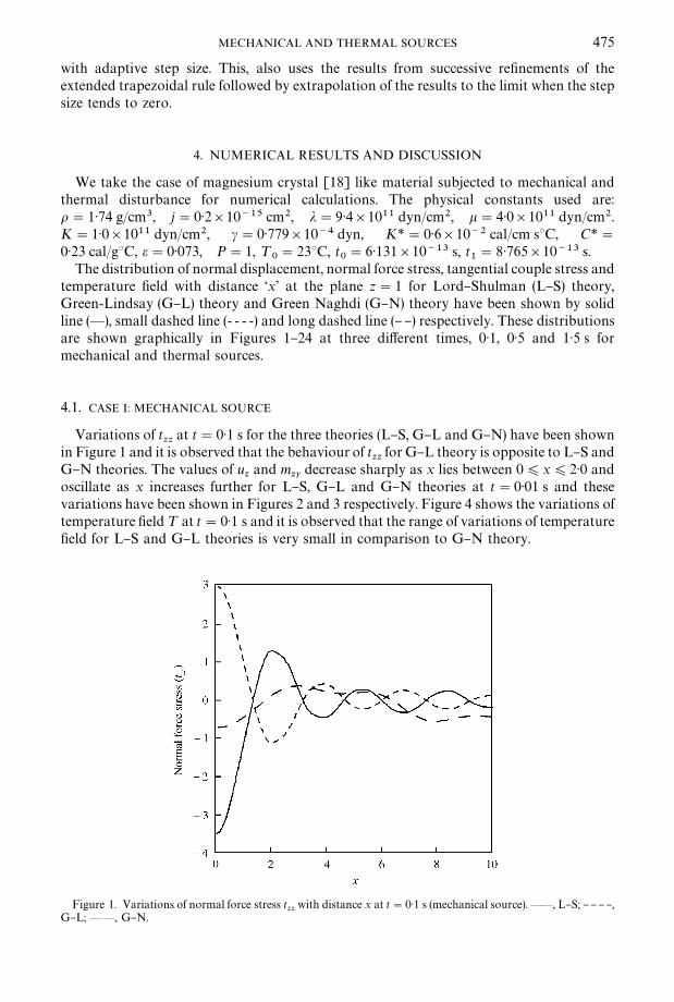
We take the case of magnesium crystal [18] like material subjected to mechanical andthermal disturbance for numerical calculations. The physical constants used are:o"1)74 g/cm3, j"0)2]10~15 cm2, j"9)4]1011 dyn/cm2, k"4)0]1011 dyn/cm2.K"1)0]1011 dyn/cm2, c"0)779]10~4 dyn, K*"0)6]10~2 cal/cm s3C, C*"0)23 cal/g3C, e"0)073, P"1, ¹
0"233C, t
0"6)131]10~13 s, t
1"8)765]10~13 s.
The distribution of normal displacement, normal force stress, tangential couple stress andtemperature "eld with distance &x' at the plane z"1 for Lord}Shulman (L}S) theory,Green-Lindsay (G}L) theory and Green Naghdi (G}N) theory have been shown by solidline (*), small dashed line (- - - -) and long dashed line (} }) respectively. These distributionsare shown graphically in Figures 1}24 at three di!erent times, 0)1, 0)5 and 1)5 s formechanical and thermal sources.
4.1. CASE I: MECHANICAL SOURCE
Variations of tzz
at t"0)1 s for the three theories (L}S, G}L and G}N) have been shownin Figure 1 and it is observed that the behaviour of t
zzfor G}L theory is opposite to L}S and
G}N theories. The values of uzand m
zydecrease sharply as x lies between 0)x)2)0 and
oscillate as x increases further for L}S, G}L and G}N theories at t"0)01 s and thesevariations have been shown in Figures 2 and 3 respectively. Figure 4 shows the variations oftemperature "eld ¹ at t"0)1 s and it is observed that the range of variations of temperature"eld for L}S and G}L theories is very small in comparison to G}N theory.
Figure 1. Variations of normal force stress tzz
with distance x at t"0)1 s (mechanical source).**, L}S; }} } },G}L; **, G}N.

Figure 2. Variations of normal displacement uz
with distance x at t"0)1 s (mechanical source). **, L}S;}} } }, G}L; **, G}N.
Figure 3. Variations of tangential couple stress mzy
with distance x at t"0)1 s (mechanical source).**, L}S;}} } }, G}L; **, G}N.
476 R. KUMAR AND S. DESWAL
Figure 5 depicts the variations of tzz
at t"0)5 s and it is noticed that the variations forL}S and G}N theories are oscillatory and lie in a very small range in comparison to G}Ltheory. The behaviour of u
zand m
zyfor three di!erent theories is similar although their
magnitude values are di!erent as x varies from 0 to 10 at t"0)5 s and these variations areshown in Figures 6 and 7 respectively. Figure 8 shows the variations of temperature "eld

Figure 4. Variations of temperature "eld ¹ with distance x at t"0)1 s (mechanical source).**, L}S; }} } },G}L; **, G}N.
Figure 5. Variations of normal force stress tzz
with distance x at t"0)5 s (mechanical source).**, L}S; }} } },G}L; **, G}N.
MECHANICAL AND THERMAL SOURCES 477
¹ at t"0)5 s and it is noticed that for G}L theory variations take place in a very smallrange in comparison to L}S and G}N theories.
Variations of tzz
at t"1)5 s for L}S and G}L theories lie in a large range and haveopposite behaviour as compared to G}N theory and these variations have been shown inFigure 9. It is further noticed that for L}S and G}L theories, there is a sharp increase in thevalues of t
zz, whereas the values decrease for G}N theory as x lies between 0)x)2)0. As

Figure 6. Variations of normal displacement uz
with distance x at t"0)5 s (mechanical source). **, L}S;}} } }, G}L; **, G}N.
Figure 7. Variations of tangential couple stress mzy
with distance x at t"0)5 s (mechanical source).**, L}S;}} } }, G}L; **, G}N.
478 R. KUMAR AND S. DESWAL
x increases further, the values of tzz
oscillate for all the three theories. Figure 10 shows thevariations of u
zat t"1)5 s and it is observed that the behaviour of u
zis similar for all the
three di!erent theories although its magnitude values are di!erent. The variations of mzy
areoscillatory for all the three theories at t"1)5 s and values of m
zylie in a very small range as
depicted in Figure 11. Figure 12 shows the behaviour of temperature "eld ¹ at t"1)5 s. It isnoticed that the variations for G}L theory lie in a very small range as compared to L}S and
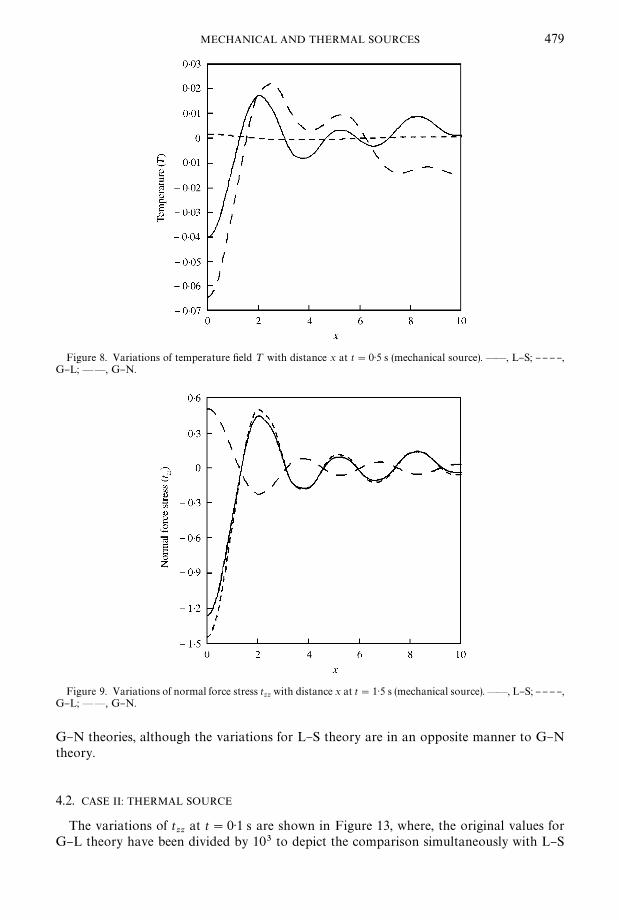
Figure 8. Variations of temperature "eld ¹ with distance x at t"0)5 s (mechanical source).**, L}S; }} } },G}L; **, G}N.
Figure 9. Variations of normal force stress tzz
with distance x at t"1)5 s (mechanical source).**, L}S; }} } },G}L; **, G}N.
MECHANICAL AND THERMAL SOURCES 479
G}N theories, although the variations for L}S theory are in an opposite manner to G}Ntheory.
4.2. CASE II: THERMAL SOURCE
The variations of tzz
at t"0)1 s are shown in Figure 13, where, the original values forG}L theory have been divided by 103 to depict the comparison simultaneously with L}S

Figure 10. Variations of normal displacement uz
with distance x at t"1)5 s (mechanical source). **, L}S;}} } }, G}L; **, G}N.
Figure 11. Variations of tangential couple stress mzy
with distance x at t"1)5 s (mechanical source).**, L}S;}} } }, G}L; **, G}N.
480 R. KUMAR AND S. DESWAL
and G}N theories and it is observed that the values for L}S theory lie in a very small rangein comparison to G}L and G}N theories. The variations of u
zat t"0)1 s are shown in
Figure 14. The values of uzfor L}S theory vary in a very short range in comparison to G}L
and G}N theories and the variations for G}L theory have been shown after dividing theoriginal values by 102. Also, the behaviour of u
zfor G}N theory is opposite from those for
L}S and G}L theories. Variations of mzy
at t"0)1 s are almost similar for three di!erent
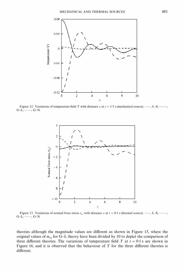
Figure 12. Variations of temperature "eld ¹ with distance x at t"1)5 s (mechanical source).**, L}S; }} } },G}L; **, G}N.
Figure 13. Variations of normal force stress tzz
with distance x at t"0)1 s (thermal source).**, L}S; }} } },G}L; **, G}N.
MECHANICAL AND THERMAL SOURCES 481
theories although the magnitude values are di!erent as shown in Figure 15, where theoriginal values of m
zyfor G}L theory have been divided by 10 to depict the comparison of
three di!erent theories. The variations of temperature "eld ¹ at t"0)1 s are shown inFigure 16, and it is observed that the behaviour of ¹ for the three di!erent theories isdi!erent.
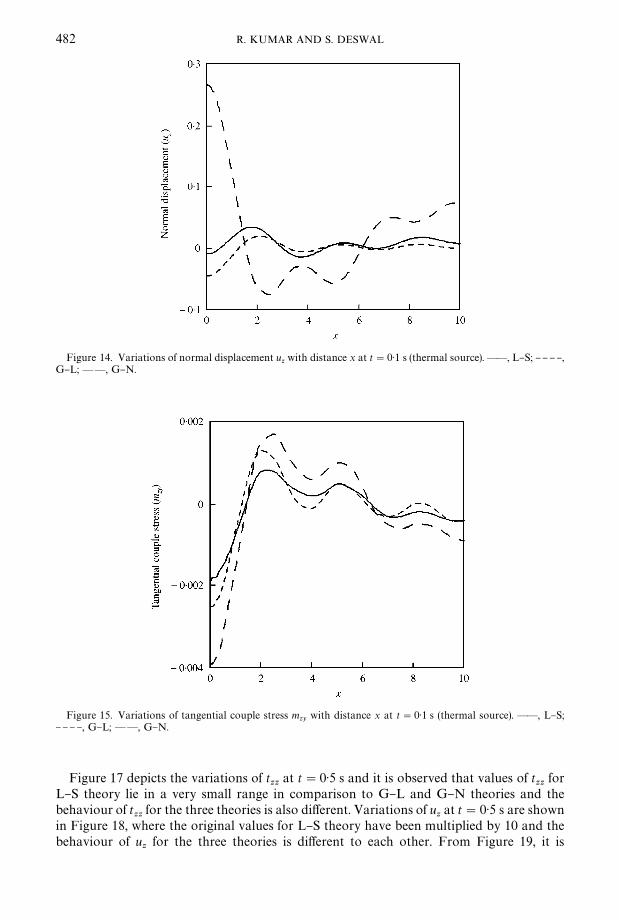
Figure 14. Variations of normal displacement uzwith distance x at t"0)1 s (thermal source).**, L}S; }} } },
G}L; **, G}N.
Figure 15. Variations of tangential couple stress mzy
with distance x at t"0)1 s (thermal source). **, L}S;}} } }, G}L; **, G}N.
482 R. KUMAR AND S. DESWAL
Figure 17 depicts the variations of tzz
at t"0)5 s and it is observed that values of tzz
forL}S theory lie in a very small range in comparison to G}L and G}N theories and thebehaviour of t
zzfor the three theories is also di!erent. Variations of u
zat t"0)5 s are shown
in Figure 18, where the original values for L}S theory have been multiplied by 10 and thebehaviour of u
zfor the three theories is di!erent to each other. From Figure 19, it is

Figure 16. Variations of temperature "eld ¹ with distance x at t"0)1 s (thermal source). **, L}S; }} } },G}L; **, G}N.
Figure 17. Variations of normal force stress tzz
with distance x at t"0)5 s (thermal source).**, L}S; }} } },G}L; **, G}N.
MECHANICAL AND THERMAL SOURCES 483
observed that variations of mzy
for L}S and G}L theories lie in a very small range incomparison to G}N theory at t"0)5 s. The range of variations of temperature "eldfor G}L and G}N theories is small in comparison to L}S theory and the variationsfor the three theories are also di!erent and these variations are shown in Figure 20 att"0)5 s.
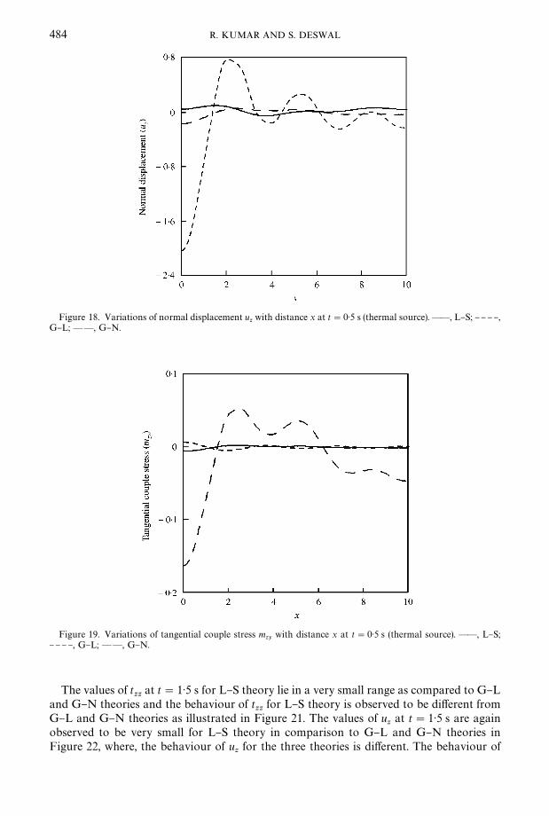
Figure 18. Variations of normal displacement uzwith distance x at t"0)5 s (thermal source).**, L}S; }} } },
G}L; **, G}N.
Figure 19. Variations of tangential couple stress mzy
with distance x at t"0)5 s (thermal source). **, L}S;}} } }, G}L; **, G}N.
484 R. KUMAR AND S. DESWAL
The values of tzz
at t"1)5 s for L}S theory lie in a very small range as compared to G}Land G}N theories and the behaviour of t
zzfor L}S theory is observed to be di!erent from
G}L and G}N theories as illustrated in Figure 21. The values of uzat t"1)5 s are again
observed to be very small for L}S theory in comparison to G}L and G}N theories inFigure 22, where, the behaviour of u
zfor the three theories is di!erent. The behaviour of
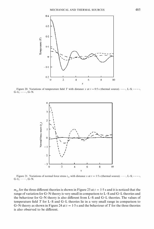
Figure 20. Variations of temperature "eld ¹ with distance x at t"0)5 s (thermal source). **, L}S; }} } },G}L; **, G}N.
Figure 21. Variations of normal force stress tzz
with distance x at t"1)5 s (thermal source).**, L}S; }} } },G}L; **, G}N.
MECHANICAL AND THERMAL SOURCES 485
mzy
for the three di!erent theories is shown in Figure 23 at t"1)5 s and it is noticed that therange of variation for G}N theory is very small in comparison to L}S and G}L theories andthe behaviour for G}N theory is also di!erent from L}S and G}L theories. The values oftemperature "eld ¹ for L}S and G}L theories lie in a very small range in comparison toG}N theory as shown in Figure 24 at t"1)5 s and the behaviour of ¹ for the three theoriesis also observed to be di!erent.

Figure 22. Variations of normal displacement uzwith distance x at t"1)5 s (thermal source).**, L}S; }} } },
G}L; **, G}N.
Figure 23. Variations of tangential couple stress mzy
with distance x at t"1)5 s (thermal source). **, L}S;}} } }, G}L; **, G}N.
486 R. KUMAR AND S. DESWAL
5. CONCLUSIONS
The magnitude of variations of the normal force stress, normal displacement, tangentialcouple stress and temperature "eld is observed to have large values at small times, whichthen become smaller and smaller with the passage of time. Also, the values of thesequantities are observed to be di!erent for the three theories (L}S, G}L and G}N) for both

Figure 24. Variations of temperature "eld ¹ with distance x at t"1)5 s (thermal source). **, L}S; }} } },G}L; **, G}N.
MECHANICAL AND THERMAL SOURCES 487
the cases and at all the three times. Since, the source applied in both the cases (mechanicaland thermal source) is instantaneous, so the range of distribution for all the expressionsbecomes small with the increase in value of distance &x'. The resulting stresses anddisplacements can be used in estimating the e!ects of a surface pressure wave.
REFERENCES
1. A. C. ERINGEN 1966 Journal of Mathematical Mechanics 15, 909}923. Linear theory ofMicropolar elasticity.
2. A. C. ERINGEN 1966 Journal of Mathematical Mechanics 16, 1}18. Theory of micropolar#uids.
3. A. C. ERINGEN 1976 A. C. Eringen editor, Continuum Physics. Vol. IV, 205}267. New York:Academic Press, Non-local polar "eld theories.
4. H. W. LORD and Y. SHULMAN 1967 Journal of the Mechanics and Physics of Solids 15, 299}306.A generalized dynamical theory of thermoelasticity.
5. A. E. GREEN and K. A. LINDSAY 1972 Journal of Elasticity 2, 1}5. Thermoelasticity.6. A. E. GREEN and P. M. NAGHDI 1991 Proceedings of the Royal Society of ¸ondon Series A. 32,
171}194. A re-examination of the basic postulate of thermodynamics.7. A. E. GREEN and P. M. NAGHDI 1992 Journal of ¹hermal Stresses 15, 253}264. On undamped heat
waves in an elastic solid.8. A. E. GREEN and P. M. NAGHDI 1993 Journal of Elasticity 31, 189}208. Thermoelasticity without
energy dissipation.9. A. C. ERINGEN 1970 Course of ¸ectures, vol. 23, CISM Udine. Berlin: Springer, Foundation of
micropolar thermoelasticity.10. W. NOWACKI 1966 Proceedings of I;¹AM Symposia, 259}278. Couple Stresses in the Theory of
Thermoelasticity.11. R. S. DHALIWAL 1971 Archives of Mechanics 23, 705}714. The steady-state axisymmetric problem
of micropolar thermoelasticity.12. R. KUMAR, T. K. CHADHA and L. DEBNATH 1987 International Journal of Mathematics and
Mathematical Science 10, 187}198. Lamb's plane problem in micropolar thermoelastic mediumwith stretch.

488 R. KUMAR AND S. DESWAL
13. R. KUMAR and B. SINGH 1996 Proceedings of the Indian Academy of Science (MathematicalScience) 106, 183}189. Wave propagation in a micropolar generalized thermoelastic body withstretch.
14. M. U. SHANKER and R. S. DHALIWAL 1975 International Journal of Engineering Science 13,121}128. Dynamic coupled thermoelastic problems in micropolar theory*I.
15. A. C. ERINGEN 1968 ¹heory of micropolar Elasticity in Fracture, Vol. II. New York: AcademicPress, Chapter 7.
16. G. HONIG and V. HIRDES 1984 Journal of Computational and Applied Mathematics 10, 113}132.A method for the numerical inversion of the Laplace transform.
17. W. H. PRESS, S. A. TEUKOLSKY, W. T. VELLERLING and B. P. FLANNERY Numerical Recipes.Cambridge: Cambridge University Press, 1986.
18. A. C. ERINGEN 1984 International Journal of Engineering Science 22, 1113}1121. Plane waves innon-local micropolar elasticity.