mechanical engineering news - plantdesignsolutions...coade mechanical engineering news january 2000...

Volume 25

Mec

hani

cal

Engi

neer

ing

New

s

FOR THE POWER,

PETROCHEMICAL AND

RELATED INDUSTRIES

The COADE Mechanical EngineeringNews Bulletin is published periodicallyfrom the COADE offices in Houston,Texas. The Bulletin is intended to provideinformation about software applicationsand development for MechanicalEngineers serving the power, petrochemi-cal and related industries. Additionally, theBulletin serves as the official notificationvehicle for software errors discovered inthose Mechanical Engineering programsoffered by COADE. (Please note, thisbulletin is published only two to threetimes per year.)

©1999 COADE, Inc. All rights reserved.

I N T H I S I S S U E :

V O L U M E 2 8 J A N U A R Y 2 0 0 0

What’s New at COADECAESAR II Version 4.20 New Features ......... 2PVElite Version 3.60 New Features ............... 2

CODECALC Version 6.20 New Features ....... 3Shows and Exhibitions ................................... 3

Technology You Can UseModeling Sway Brace Assemblies in

CAESAR II ................................................. 3Hydrodynamic Loading of Piping Systems .... 5

A Comparison of Wind Load Calculationsper ASCE 93 and ASCE 95 ..................... 10

Layouts in AutoCAD 2000 and

CADWorx/PIPE ........................................ 13PC Hardware for the Engineering User

(Part 28) ................................................... 17

Program SpecificationsCAESAR II Notices ...................................... 18TANK Notices ............................................... 19

CODECALC Notices .................................... 19PVElite Notices ............................................ 20

HydrodynamicLoading ofPiping Systems

> see story page 5

Layouts inAutoCAD 2000 &CADWorx/PIPE

> see story page 13

CAESAR IIVersion 4.20New Features

> see story page 2

CAESAR II Receives TD12 Approvalby Transco

On November 30, 1999, following a long and rigorous validation process,the Stress Analysis Workgroup of Transco officially approved CAESAR IIfor use on projects requiring the IGE/TD/12 piping code, “PipeworkStress Analysis for Gas Industry Plant”. Transco is the Gas Transportationarm of the British Gas Group. CAESAR II thus becomes the first andonly commercially available pipe stress analysis program so accepted byTransco. Note that only CAESAR II Version 4.10 Build 991201(December 1, 1999) and later is covered by this acceptance.

ATTENTION:Users of Green External Software Locks!

All new COADE products released after July 2000 will no longer supportthe old SSI (Software Security, Inc.) ESLs since this company is no longerin business. Any users who are current on their maintenance and are nowusing one of these ESLs (identified by their green color) should contactCOADE to arrange for a replacement ESL.

All COADE products released after January 2000 will remind any userswho still have green ESLs of this situation. Please contact COADE as perthe instruction on the screen so that this transition can be accomplished witha minimum of effort.

COADE Mechanical Engineering News January 2000

2

CAESAR II Version 4.20New Features

By: Richard Ay

CAESAR II Version 4.20 is nearing completion. Some of themajor new features of this release are listed in the table below.

CAESAR II Version 4.20 Features New Input Graphics - utilizes a true 3D library, enabling graphic element selection Completely revised material data base, including Code updates. Hydrodynamic loading for offshore applications. This includes the Airy, Stokes 5th, and Stream Function wave theories, as well as Linear and Power Law current profiles. Wind analysis expanded to handle up to 4 wind load cases New piping codes: B31.4 Chapter IX, B31.8 Chapter VIII, and DNV (ASD) A wave scratchpad - see the recommended theory graphically, or plot the particle data for the specified wave. Updated piping codes: B31.3, B31.4 Automatic Dynamic DLF Plotting Hydra expansion joint data bases PCF Interface

The new input graphics provide a much faster drawing response,noticeably speeding up the graphics operations. The default drawingmode will be a 3D rendered view. New capabilities of this graphicslibrary will allow the user to click on an element and pull up theassociated input spreadsheet. Additionally, the graphic can beannotated with user defined notes for printing purposes. A sampleinput graphic generated from this new library is shown in the figurebelow. The new input graphics are provided alongside the old ones,since all functions have not be provided in this environment yet.

Details of the hydrodynamic (wave and current) capabilities arediscussed in a later article in this newsletter. Several piping codeshave been added for the offshore implementation of hydrodynamicloads (B31.4 Chapter XI, B31.8 Chapter VIII, and DNV). Inaddition, the load case editor has been modified to accommodate upto four wave/current cases and up to four wind cases.

For users of the “force spectrum dynamics”, Version 4.20 willprovide automatic plotting of the computed DLF curve. Thisplotting occurs automatically once the time pulse has been entered.The resulting numeric DLF data and its plot are shown side by side,as depicted in the figure below.

The PCF interface was actually first distributed in the 990617 buildof Version 4.10. We don’t normally include new capabilities orfeatures in intermediate builds, but we felt this one was worthdistributing before the next major release. The PCF interface readsa PCF neutral file and creates a CAESAR II model. Any CADpackage which can create a PCF file, can be used to createCAESAR II piping geometries.

PVElite Version 3.60 New FeaturesBy: Scott Mayeux

PVElite Version 3.60 will be ready to ship before the end of 1999.A number of new capabilities have been added for this version, inaddition to the ASME code updates. These new features are listedin the table below.

PVElite Version 3.60 Features A-99 addenda changes have been incorporated, including the higher allowable stresses for Div. 1 The pre 99 addenda is available as an option (uses the 98 addenda material database, etc.) Other FVC nozzles such as types F, V1, V2, and V3 are now included (with or without nut relief) Nozzle calculations in ANSI blind flanges can now be performed (full area replacement) An ANSI flange dimension lookup feature has been added Required flange thickness calculations based on Rigidity considerations are included A saddle copy feature has been incorporated The program’s documentation is now available on-line in PDF format Several enhancements to the user interface have been made Dimensional Solutions Foundation 3-D interface has been added MAWP and MAPnc can now be manually defined The 3/32 min. thickness requirement based on the Service type (Unfired Steam) is accounted for The Maximum hydrotest pressure is computed in the case of overstressed geometries The ESL will automatically be updated for current users (obviating the need for the phone call) An option for the pneumatic hydrotest type has been added The material database editor can select materials from the database for editing purposes

Additional changes and updates have also been made to thecomponent modules of PVElite, which are also included inCODECALC Version 6.20.

January 2000 COADE Mechanical Engineering News

3

CODECALC Version 6.20New Features

By: Scott Mayeux

CODECALC Version 6.20 will be ready to ship before the end of1999. A number of new capabilities have been added for thisversion, in addition to the ASME code updates. These new featuresare listed in the table below.

C O D EC A LC V ersion 6 .20 Features A -99 ad denda changes have been incorpora ted , inc luding the h igher a llowable stresses for D iv . 1 T he pre 99 ad denda is available as an option (uses the 98 addenda m aterial da tabase, etc.) R equired flange th ickness ca lculations based on R igid ity considerations T EM A E ighth editio n changes are inc luded C ode C ase 22 60 has been add ed T he C odeCalc U ser in terface has been re-written and now has lower mem ory requirem ents C alcula tions per W R C 297 have been added A ppendix Y calcula tions are now also included T he m aterial database editor can se lec t m aterials from the database for ed iting purp oses T he E SL will automatica lly b e updated for current users (obviating the need for the phone call) T hick W alled C ylinder and Sphere equations are im plem ented per Ap pendix 1 T he output processo r has been re-worked and stream lined

Shows and ExhibitionsBy: Richard Ay

COADE attends industry trade shows and exhibitions as a normalbusiness activity. The benefits of attending these events are: contactwith existing customers, introduction of the software to prospectiveusers, introduction of new features to the industry. Recently COADEattended two shows, hosted by our local dealers in the regions.

The Offshore Europe show was held in Aberdeen, Scotland fromSeptember 7 through September 10, 1999. COADE’s Tom VanLaan helped staff Fern Computer Consultancy’s booth for thisevent. At this show, COADE demonstrated the new offshorefeatures of CAESAR II. The four day show attracted over 25,000attendees, including many long-time COADE customers.

The Arab Oil and Gas show was held in Dubai, U.A.E. fromOctober 16 through October 19, 1999. COADE’s Richard Ayhelped staff ImageGrafix’s booth for this event. At this show, twopresentations were made. The first presentation detailed the newhydrodynamic (offshore) features of CAESAR II Version 4.20.The second presentation was an “all product” demonstration,covering the complete line of COADE software products.

The ImageGrafix Booth at the Arab Oil & Gas Show,Dubai, U.A.E.

COADE has also attended a number of CAD-centric shows, inorder to showcase CADWorx, our piping design and draftingsoftware. Among others, Vornel Walker and Robert Wheat haveattended AEC Systems, the Autodesk “One Team” Conferences (inLos Angeles and Nice, France), and the World Wide Food Expothis year.

Visitors to these exhibitions have the opportunity to discuss softwareissues, concerns, and needs first hand with the local dealer offeringsupport in the region, as well as the developers of the software.These exhibitions provide an excellent forum for informationexchange and education. A list of the exhibitions at which COADEpersonnel will be present is maintained on the COADE web site.These events are well worth attending.

Modeling Sway Brace Assembliesin CAESAR II

By: Griselda Mani

Vibration in a piping system is an undesirable movement that adesigner must often consider. Vibration from equipment such aspumps, turbines and vessels can usually be anticipated and prevented.However, periodic motion or rapid oscillations of piping componentscannot always be anticipated; it may cause serious failure in a shortperiod of time or fatigue failure if of long duration. A recommendedsolution for controlling this type of vibration in a piping system isthe use of a sway brace assembly.

The sway brace is commonly used to allow unrestrained thermalmovements while “tuning” the system dynamically to eliminatevibration. In this respect, the sway brace resembles a spring: it maybe pre-loaded in the cold (installed) position, so that after thermalpipe growth it reaches the neutral position and the load on thesystem in the operating condition is zero or negligible.


4

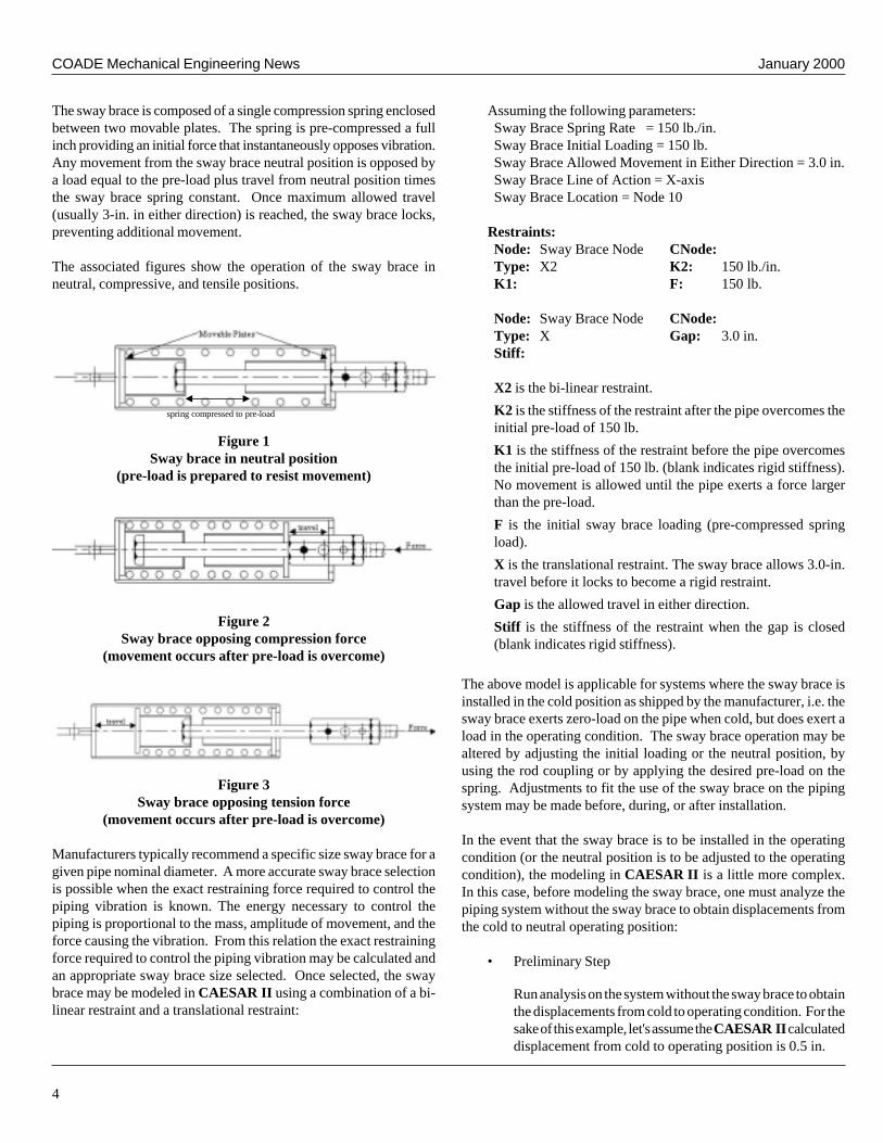
The sway brace is composed of a single compression spring enclosedbetween two movable plates. The spring is pre-compressed a fullinch providing an initial force that instantaneously opposes vibration.Any movement from the sway brace neutral position is opposed bya load equal to the pre-load plus travel from neutral position timesthe sway brace spring constant. Once maximum allowed travel(usually 3-in. in either direction) is reached, the sway brace locks,preventing additional movement.

The associated figures show the operation of the sway brace inneutral, compressive, and tensile positions.

spring compressed to pre-load

Figure 1Sway brace in neutral position

(pre-load is prepared to resist movement)

Figure 2Sway brace opposing compression force

(movement occurs after pre-load is overcome)

Figure 3Sway brace opposing tension force

(movement occurs after pre-load is overcome)

Manufacturers typically recommend a specific size sway brace for agiven pipe nominal diameter. A more accurate sway brace selectionis possible when the exact restraining force required to control thepiping vibration is known. The energy necessary to control thepiping is proportional to the mass, amplitude of movement, and theforce causing the vibration. From this relation the exact restrainingforce required to control the piping vibration may be calculated andan appropriate sway brace size selected. Once selected, the swaybrace may be modeled in CAESAR II using a combination of a bi-linear restraint and a translational restraint:

Assuming the following parameters:Sway Brace Spring Rate = 150 lb./in.Sway Brace Initial Loading = 150 lb.Sway Brace Allowed Movement in Either Direction = 3.0 in.Sway Brace Line of Action = X-axisSway Brace Location = Node 10

Restraints:Node: Sway Brace Node CNode:Type: X2 K2: 150 lb./in.K1: F: 150 lb.

Node: Sway Brace Node CNode:Type: X Gap: 3.0 in.Stiff:

X2 is the bi-linear restraint.K2 is the stiffness of the restraint after the pipe overcomes theinitial pre-load of 150 lb.K1 is the stiffness of the restraint before the pipe overcomesthe initial pre-load of 150 lb. (blank indicates rigid stiffness).No movement is allowed until the pipe exerts a force largerthan the pre-load.F is the initial sway brace loading (pre-compressed springload).X is the translational restraint. The sway brace allows 3.0-in.travel before it locks to become a rigid restraint.Gap is the allowed travel in either direction.Stiff is the stiffness of the restraint when the gap is closed(blank indicates rigid stiffness).

The above model is applicable for systems where the sway brace isinstalled in the cold position as shipped by the manufacturer, i.e. thesway brace exerts zero-load on the pipe when cold, but does exert aload in the operating condition. The sway brace operation may bealtered by adjusting the initial loading or the neutral position, byusing the rod coupling or by applying the desired pre-load on thespring. Adjustments to fit the use of the sway brace on the pipingsystem may be made before, during, or after installation.

In the event that the sway brace is to be installed in the operatingcondition (or the neutral position is to be adjusted to the operatingcondition), the modeling in CAESAR II is a little more complex.In this case, before modeling the sway brace, one must analyze thepiping system without the sway brace to obtain displacements fromthe cold to neutral operating position:

• Preliminary Step

Run analysis on the system without the sway brace to obtainthe displacements from cold to operating condition. For thesake of this example, let's assume the CAESAR II calculateddisplacement from cold to operating position is 0.5 in.


5

• Model the sway braceAssume the following parameters:

Sway Brace Spring Rate = 150 lb./in.Sway Brace Initial Loading = 150 lb.Sway Brace Allowed Movement in Either Direction =3 in.

Restraints:Node: 10 CNode: 101Type: X2 K2: 150 lb./in.K1: F: 150 lb.

Node: 10 CNode: 101Type: X Gap: 3.0 in.Stiff:

Displacements:Node: 101DX2: 0.5 in.

• Include the applied displacement D2 (vector 2) in both theSUS and OPE load cases.

Typically as shown:

Load Case 1 - W+P1+T1+D1+F1+D2 (OPE)Load Case 2 - W+P1+F1+D2 (SUS)Load Case 3 - DS1-DS2 (EXP)

In the SUS case the displacement D2 (vector 2) represents the pre-load in cold position. Under shutdown conditions, the pipe returnsto its cold position and the brace exerts a force as previouslydescribed.

Sustained case restraint loads on sway brace = Pre-Load + HotDeflection * Spring Rate

In OPE the displacement allows thermal expansion and the swayassumes neutral position exerting zero or negligible load on thepipe.

Operating case restraint loads on sway brace =~ 0.0 (does notrestrain thermal expansion)

Engineers and designers in search of solutions to vibration problemsreadily recognize the importance and functions of the sway brace.The assembly is easy to handle, select and adjust, and now, easy tomodel in CAESAR II.

Hydrodynamic Loading ofPiping Systems

By: Richard Ay

Ocean waves are generated by wind and propagate out of thegenerating area. The generation of ocean waves is dependent on thewind speed, the duration of the wind, the water depth, and thedistance over which the wind blows. This distance over which thewind blows is referred to as the fetch length. There are a variety oftwo dimensional wave theories proposed by various researchers,but the three most widely used are the Airy (linear) wave theory,Stokes 5th Order wave theory, and Dean’s Stream Function wavetheory. The later two theories are non-linear wave theories andprovide a better description of the near-surface effects of the wave.

(The term “two dimensional” refers to the “uni-directional” wave.One dimension is the direction the wave travels, and the otherdimension is vertical through the water column. Two dimensionalwaves are not found in the marine environment, but are somewhateasy to define and determine properties for, in a deterministic sense.In actuality, waves undergo spreading, in the third dimension. Thiscan be easily understood by visualizing a stone dropped in a pond.As the wave spreads, the diameter of the circle increases. Inaddition to wave spreading, a real sea state includes waves ofvarious periods, heights, and lengths. In order to address theseactual conditions, a deterministic approach cannot be used. Instead,a sea spectrum is utilized, which may also include a spreadingfunction. As there are various wave theories, there are various seaspectra definitions. The definition and implementation of sea spectraare usually employed in dynamic analysis. Sea Spectra and dynamicanalysis, which has been left for a future implementation ofCAESAR II , will not be discussed in this article.)

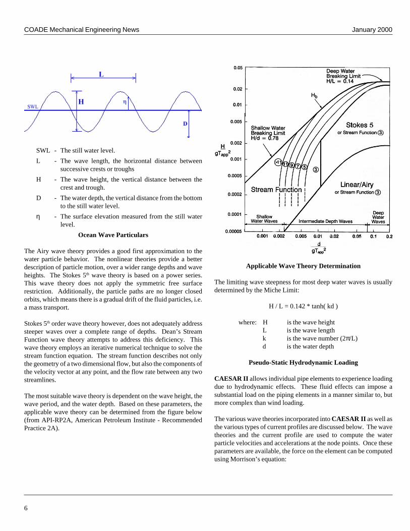
The linear or Airy wave theory assumes the free surface is symmetricabout the mean water level. Furthermore, the water particle motionis a closed circular orbit, the diameter of which decays with depth.(The term circular should be taken loosely here, the orbit variesfrom circular to elliptical based on whether the wave is in shallow ordeep water.) Additionally, for shallow water waves, the waveheight to depth ratio (H/D) is limited to 0.78, to avoid breaking.(None of the wave theories address breaking waves!) The figurebelow shows a typical wave and associated hydrodynamicparameters.


6

SWL - The still water level.L - The wave length, the horizontal distance between

successive crests or troughsH - The wave height, the vertical distance between the

crest and trough.D - The water depth, the vertical distance from the bottom

to the still water level.η - The surface elevation measured from the still water

level.Ocean Wave Particulars

The Airy wave theory provides a good first approximation to thewater particle behavior. The nonlinear theories provide a betterdescription of particle motion, over a wider range depths and waveheights. The Stokes 5th wave theory is based on a power series.This wave theory does not apply the symmetric free surfacerestriction. Additionally, the particle paths are no longer closedorbits, which means there is a gradual drift of the fluid particles, i.e.a mass transport.

Stokes 5th order wave theory however, does not adequately addresssteeper waves over a complete range of depths. Dean’s StreamFunction wave theory attempts to address this deficiency. Thiswave theory employs an iterative numerical technique to solve thestream function equation. The stream function describes not onlythe geometry of a two dimensional flow, but also the components ofthe velocity vector at any point, and the flow rate between any twostreamlines.

The most suitable wave theory is dependent on the wave height, thewave period, and the water depth. Based on these parameters, theapplicable wave theory can be determined from the figure below(from API-RP2A, American Petroleum Institute - RecommendedPractice 2A).

Applicable Wave Theory Determination

The limiting wave steepness for most deep water waves is usuallydetermined by the Miche Limit:

H / L = 0.142 * tanh( kd )

where: H is the wave heightL is the wave lengthk is the wave number (2π/L)d is the water depth

Pseudo-Static Hydrodynamic Loading

CAESAR II allows individual pipe elements to experience loadingdue to hydrodynamic effects. These fluid effects can impose asubstantial load on the piping elements in a manner similar to, butmore complex than wind loading.

The various wave theories incorporated into CAESAR II as well asthe various types of current profiles are discussed below. The wavetheories and the current profile are used to compute the waterparticle velocities and accelerations at the node points. Once theseparameters are available, the force on the element can be computedusing Morrison’s equation:


7

F = 1/2 * ρ * Cd * D * U * |U| + π/4 * ρ * Cm * D2 * A

where ρ - is the fluid densityCd - is the drag coefficientD - is the pipe diameterU - is the particle velocityCm - is the inertial coefficientA - is the particle acceleration

The particle velocities and accelerations are vector quantities whichinclude the effects of any applied waves or currents. In addition tothe force imposed by Morrison’s equation, piping elements are alsosubjected to a lift force and a buoyancy force. The lift force isdefined as the force acting normal to the plane formed by thevelocity vector and the element’s axis. The lift force is defined as:

Fl = 1/2 * ρ * Cl * D * U2

where ρ - is the fluid densityCl - is the lift coefficientD - is the pipe diameterU - is the particle velocity

The buoyancy force acts upward, and is equal to the weight of thefluid volume displaced by the element. The buoyancy effect isautomatically included in all load cases which include weight.

Once the force on a particular element is available, it is placed in thesystem load vector just as any other load is. A standard solution isperformed on the system of equations which describe the pipingsystem. (The piping system can be described by the standard finiteelement equation:

[K] {x} = {f}

where [K] - is the global stiffness matrix for theentire system

{x} - is the displacement / rotation vectorto solve for

{f} - is global load vector

The element loads generated by the hydrodynamic effects are placedin their proper locations in {f}, similar to weight, pressure, andtemperature. Once [K] and {f} are finalized, a standard finiteelement solution is performed on this system of equations. Theresulting displacement vector {x} is then used to compute elementforces, and these forces are then used to compute the elementstresses.)

Except for the buoyancy force, all other hydrodynamic forces actingon the element are a function of the particle velocities andaccelerations.

AIRY Wave Theory Implementation

Airy wave theory is also known as “linear” wave theory, due to theassumption that the wave profile is symmetric about the mean waterlevel. Standard Airy wave theory allows for the computation of thewater particle velocities and accelerations between the mean surfaceelevation and the bottom. The Modified Airy wave theory allowsfor the consideration of the actual free surface elevation in thecomputation of the particle data. CAESAR II includes both thestandard and modified forms of the Airy wave theory.

To apply the Airy wave theory, several descriptive parametersabout the wave must be given. These values are then used to solvefor the wave length, which is a characteristic parameter of eachunique wave. CAESAR II uses Newton-Raphson iteration todetermine the wave length by solving the dispersion relation, shownbelow:

L = (gT2 / 2π) * tanh(2πD / L)

where g - is the acceleration of gravityT - is the wave periodD - is the mean water depthL - is the wave length to be solved for

Once the wave length (L) is known, the other wave particulars ofinterest may be easily determined. The parameters determined andused by CAESAR II are: the horizontal and vertical particlevelocities ( UX and UY ), the horizontal and vertical particleacceleration ( AX and AY ), and the surface elevation (ETA) above(or below) the mean water level. The equations for these parameterscan be found in any standard text (such as those listed at the end ofthis section) which discusses ocean wave theories, and thereforewill not be repeated here.

STOKES Wave Theory Implementation

The Stokes wave is a 5th order gravity wave, and hence non-linearin nature. The solution technique employed by CAESAR II isdescribed in a paper published by Skjelbreia and Hendrickson ofthe National Engineering Science Company of Pasadena California,in 1960. The standard formulation as well as a modified formulation(to the free surface) are available in CAESAR II.

The solution follows a procedure very similar to that used in theAiry wave; characteristic parameters of the wave are determined byusing Newton-Raphson iteration, followed by the determination ofthe water particle values of interest.


8

The Newton-Raphson iteration procedure solves two non-linearequations for the constants beta and lambda. Once these values areavailable, the other twenty constants can be computed. After all ofthe constants are known, CAESAR II can compute: the horizontaland vertical particle velocities (UX and UY), the horizontal andvertical particle acceleration (AX and AY), and the surface elevation(ETA) above the mean water level.

Stream Function Wave Theory Implementation

The solution to Dean’s Stream Function Wave Theory employed byCAESAR II is described in the text by Sarpkaya and Isaacson. Aspreviously mentioned, this is a numerical technique to solve thestream function. The solution subsequently obtained, provides thehorizontal and vertical particle velocities (UX and UY), the horizontaland vertical particle acceleration (AX and AY), and the surfaceelevation (ETA) above the mean water level.

Ocean Currents

In addition to the forces imposed by ocean waves, piping elementsmay also be subjected to forces imposed by ocean currents. Thereare three different ocean current models in CAESAR II; linear,piece-wise, and a power law profile.

The linear current profile assumes that the current velocity throughthe water column varies linearly from the specified surface velocity(at the surface) to zero (at the bottom). The piece-wise linearprofile employs linear interpolation between specific “depth/velocity” points specified by the user. The power law profiledecays the surface velocity to the 1/7 power.

While waves produce unsteady flow, where the particle velocitiesand accelerations at a point constantly change, current produces asteady, non-varying flow.

Technical Notes on CAESAR II Hydrodynamic Loading

The input parameters necessary to define the fluid loading aredescribed in detail in the next section. The basic parametersdescribe the wave height and period, and the current velocity. Themost difficult to obtain, and also the most important parameters, arethe drag, inertia, and lift coefficients, Cd, Cm, and Cl. Based on therecommendations of API RP2A and DNV (Det Norske Veritas),values for Cd range from 0.6 to 1.2, values for Cm range from 1.5 to2.0. Values for Cl show a wide range of scatter, but the approximatemean value is 0.7.

The inertia coefficient Cm is equal to one plus the added masscoefficient Ca. This added mass value accounts for the mass of thefluid assumed to be entrained with the piping element.

In actuality, these coefficients are a function of the fluid particlevelocity, which varies over the water column. In general practice,two dimensionless parameters are computed which are used toobtain the Cd, Cm, and Cl values from published charts. The firstdimensionless parameter is the Keulegan-Carpenter Number, K. Kis defined as:

K = Um * T / D

where: Um - is the maximum fluid particle velocityT - is the wave periodD - is the characteristic diameter of the

element.

The second dimensionless parameter is the Reynolds number, Re.Re is defined as

Re = Um * D / ν

where Um - is the maximum fluid particle velocityD - is the characteristic diameter of the

elementν - is the kinematic viscosity of the fluid

(1.26e-5 ft2/sec for sea water).

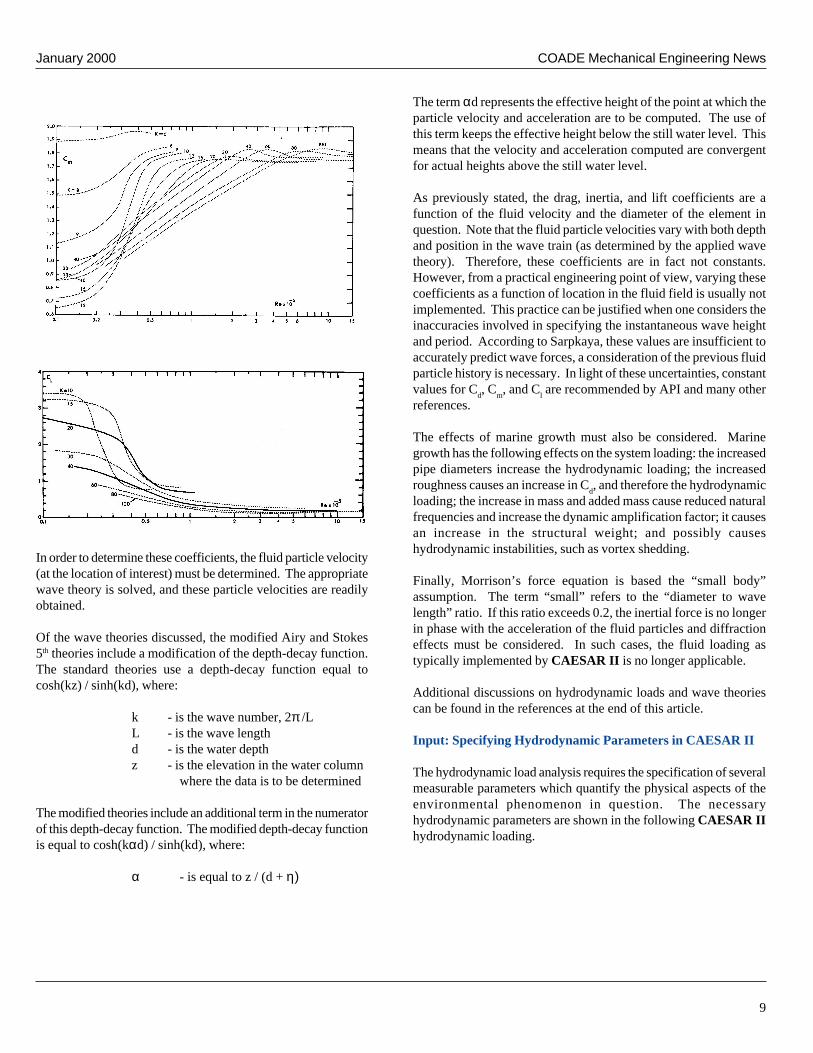
Once K and Re are available, charts are used to obtain Cd, Cm, andCl. (See Mechanics of Wave Forces on Offshore Structures by T.Sarpkaya, Figures 3.21, 3.22, and 3.25 for example charts, whichare shown in the figures below.)


9

In order to determine these coefficients, the fluid particle velocity(at the location of interest) must be determined. The appropriatewave theory is solved, and these particle velocities are readilyobtained.

Of the wave theories discussed, the modified Airy and Stokes5th theories include a modification of the depth-decay function.The standard theories use a depth-decay function equal tocosh(kz) / sinh(kd), where:

k - is the wave number, 2π /LL - is the wave lengthd - is the water depthz - is the elevation in the water column

where the data is to be determined

The modified theories include an additional term in the numeratorof this depth-decay function. The modified depth-decay functionis equal to cosh(kαd) / sinh(kd), where:

α - is equal to z / (d + η)

The term αd represents the effective height of the point at which theparticle velocity and acceleration are to be computed. The use ofthis term keeps the effective height below the still water level. Thismeans that the velocity and acceleration computed are convergentfor actual heights above the still water level.

As previously stated, the drag, inertia, and lift coefficients are afunction of the fluid velocity and the diameter of the element inquestion. Note that the fluid particle velocities vary with both depthand position in the wave train (as determined by the applied wavetheory). Therefore, these coefficients are in fact not constants.However, from a practical engineering point of view, varying thesecoefficients as a function of location in the fluid field is usually notimplemented. This practice can be justified when one considers theinaccuracies involved in specifying the instantaneous wave heightand period. According to Sarpkaya, these values are insufficient toaccurately predict wave forces, a consideration of the previous fluidparticle history is necessary. In light of these uncertainties, constantvalues for Cd, Cm, and Cl are recommended by API and many otherreferences.

The effects of marine growth must also be considered. Marinegrowth has the following effects on the system loading: the increasedpipe diameters increase the hydrodynamic loading; the increasedroughness causes an increase in Cd, and therefore the hydrodynamicloading; the increase in mass and added mass cause reduced naturalfrequencies and increase the dynamic amplification factor; it causesan increase in the structural weight; and possibly causeshydrodynamic instabilities, such as vortex shedding.

Finally, Morrison’s force equation is based the “small body”assumption. The term “small” refers to the “diameter to wavelength” ratio. If this ratio exceeds 0.2, the inertial force is no longerin phase with the acceleration of the fluid particles and diffractioneffects must be considered. In such cases, the fluid loading astypically implemented by CAESAR II is no longer applicable.

Additional discussions on hydrodynamic loads and wave theoriescan be found in the references at the end of this article.

Input: Specifying Hydrodynamic Parameters in CAESAR II

The hydrodynamic load analysis requires the specification of severalmeasurable parameters which quantify the physical aspects of theenvironmental phenomenon in question. The necessaryhydrodynamic parameters are shown in the following CAESAR IIhydrodynamic loading.


10

Details of this input screen can be found in the programdocumentation. Once the wave parameters have been defined, the“plot” button on the tool bar (the far right button in the figure above)will activate the Wave Wizard. This module will plot the“Recommended Wave Theory” diagram, including the location ofthe specific wave just defined. This diagram shows exactly wherethe specified wave falls on the chart, as shown in the figure below.

The Wave Wizard can produce other plots of the data for thisspecific wave, as well as display the numeric data tables whichcorrespond to these plots. The “View Data Table” button at thebottom of the screen brings up the numeric data in tabular form.This data includes the free surface elevation as a function of wavephase, and tables of horizontal and vertical velocities andaccelerations as a function of wave phase and water depth. Anexample plot (obtained by selecting from the drop list in the figureabove) shown below.

A Comparison of Wind LoadCalculations per ASCE 93and ASCE 95

By: Scott Mayeux

Frequently in the design of vertical and horizontal pressure vessels,the need for computing loads on these and other structures due tothe effects of wind is a necessity. Air can be thought of as a fluid oflow viscosity. When air moves around an obstacle, its kineticenergy is given up to the structure that is resisting the wind. Becauseof this transfer of momentum and energy, forces are placed on astructure that cause bending and other loads to arise. It is theseloads that we must account for in the design of pressure vessels,most notably vertical pressure vessels. In this article we willexplore the equations that are used in the computation of wind loadsaccording to the ASCE 95 and 93 design codes. Of course there aremany wind design codes that are in use world wide, but the ASCEcodes are commonly used in the United States and we will concentrateon how these codes develop loads due wind and compare them.The discussion of the ASCE 95 code will be followed by thediscussion of the ASCE 93 code.

From physics, the kinetic energy of a moving particle is expressedby the following equation:

Ke = 1/2 M V2

Where M is the mass of the particle and V is the velocity. In UScustomary units the mass is expressed in units of lb. and velocity isexpressed in units of feet per second. Please note that in this systemof units the gravitational acceleration constant of 32.2 must beproperly applied to the mass M.


11

Obtaining the kinetic energy term is step 1 in the determination ofthe wind pressure at a given elevation. The term is as follows:

Constant = 00256.03600

52802.32

0765.021 2

2

=

×

shr

mift

hrmi

fts

ftculb

The constant that uses the value of 0.0765, reflects the mass densityof air at standard atmospheric pressure and a temperature of 59degrees F. This constant is used in the following equation of qz,which is the wind pressure at an arbitrary elevation (z). qz isexpressed by the following equation:

qz = 0.00256(Kz)(Kzt)(V2)(I) units: Pound per square foot (psf)

Where Kz - velocity pressure coefficient,Kzt - topographic factor,V - basic wind speedI - importance factor.

The term Kz in turn is defined by the following equation(s):

For elevations below 15 feet, Kz = 2.01*( 15/zg)2/alpha. For elevationsabove 15 feet, Kz = 2.01*(z/zg) 2/alpha. Values of alpha and zg areshown in the table below:

Exposure Category Constants

Exp. Category alpha Zg(ft)

A 5.0 1500B 7.0 1200C 9.5 900D 11.5 700

The exposure categories in the ASCE code are explained in paragraph6.5.3. The exposure category pertains to the amount of obstructionthe structure is shielded from. For example, a vertical structure thatlies along a flat unobstructed plain will feel the full effect of thewind. While a structure in the middle of a large city center withplenty of shielding will not feel the full effect of the wind. Anexposure D is the most conservative while A is the least conservative.

The topographic factor Kzt involves computing the speed up effectof the wind blowing over a hill or some other type of escarpment.For most computations in this industry, Kzt is taken to be 1.0.

V is defined as the basic wind speed. The minimum value of V is 70miles per hour. Along hurricane oceanlines V increases substantiallyto 120 mph or higher. Note that since this term is squared, it has abig impact on the final wind pressure qz.

The final term in the equation of qz is I. I is the importance factor.It accounts for the degree of loss of life and damage to property. Ican vary between 0.87 to values of 1.15 or greater.

Now that we are familiar with all of the terms needed to compute qz,lets look at a sample calculation.

Given: Exposure C, V = 100 mph, I = 1.15, z = 50 ft.

From the table alpha is 9.5 and zg is 900 ft. Consequently kz =2.01*(50/900) 2/9.5. kz is therefore equal to 1.098. qz =0.00256(1.0938)(1)(100 * 100)(1.15). Thusly at an elevation of 50feet the computed wind pressure is 32.2 lbs/sq ft. Once the windpressure at the target elevation has been computed the relationForce = pressure * area is used to determine a single concentratedforce F at this elevation.

PVElite uses this methodology to compute loads at the wind centroidof each element (shell course). There are two more terms that areinvolved in the final computation of the force. These terms are theGust Response Factor and the shape factor. Vertical pressurevessels are typically round and smooth and have a shape factor of0.6 to 0.8. The other term is the gust response factor G. The gustresponse factor accounts for the fact that the wind “gusts” or speedsup periodically. This factor is a computed constant for the entirestructure and depends on its dynamic sensitivity. Gust effect factorsare discussed in paragraph 6.6 of ASCE 95.

After the wind pressure at each elevation has been computed, thearea of each element must also be computed. The wind pressuretimes the area results in a force at elevation z. This force times adistance to the support point results in a bending moment. Thestress on the cross section due to this moment should also beinvestigated.

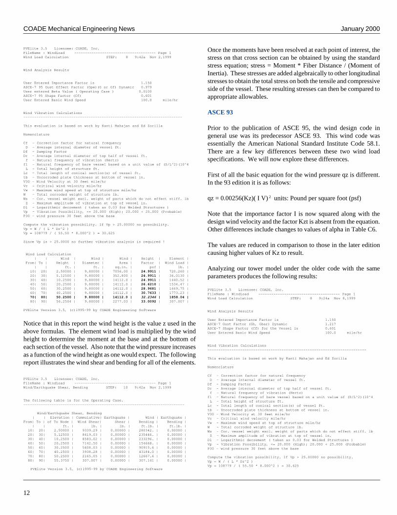
The following sample shows a PVElite sample model with a windloading and shear and bending report.


12

PVElite 3.5 Licensee: COADE, Inc.FileName : WindLoad —————————————————————————————————————— Page 1Wind Load Calculation STEP: 8 9:42a Nov 2,1999

Wind Analysis Results

User Entered Importance Factor is 1.150ASCE-7 95 Gust Effect Factor (Ope)(G or Gf) Dynamic 0.979User entered Beta Value ( Operating Case ) 0.0100ASCE-7 95 Shape Factor (Cf) 0.601User Entered Basic Wind Speed 100.0 mile/hr

Wind Vibration Calculations—————————————————————————————————————————————————————————————————————————

This evaluation is based on work by Kanti Mahajan and Ed Zorilla

Nomenclature

Cf - Correction factor for natural frequency D - Average internal diameter of vessel ft.Df - Damping FactorDr - Average internal diameter of top half of vessel ft. f - Natural frequency of vibration (Hertz)f1 - Natural frequency of bare vessel based on a unit value of (D/L^2)(10^4 L - Total height of structure ft.Lc - Total length of conical section(s) of vessel ft.tb - Uncorroded plate thickness at bottom of vessel in.V30 - Wind Velocity at 30 feet mile/hrVc - Critical wind velocity mile/hrVw - Maximum wind speed at top of structure mile/hrW - Total corroded weight of structure lb.Ws - Cor. vessel weight excl. weight of parts which do not effect stiff. lb Z - Maximum amplitude of vibration at top of vessel in.Dl - Logarithmic decrement ( taken as 0.03 for Welded Structures )Vp - Vibration Possibility, <= 20.000 (High); 20.000 < 25.000 (Probable)P30 - wind pressure 30 feet above the base

Compute the vibration possibility. If Vp > 25.00000 no possibility.Vp = W / ( L * Dr^2 )Vp = 108779 / ( 55.50 * 8.000^2 ) = 30.625

Since Vp is > 25.0000 no further vibration analysis is required !

Wind Load Calculation | | Wind | Wind | Wind | Height | Element | From| To | Height | Diameter | Area | Factor | Wind Load | | | ft. | ft. | sq.in. | psf | lb. | 10| 20| 2.50000 | 9.80000 | 7056.00 | 24.9911 | 720.260 | 20| 30| 5.12500 | 9.80000 | 352.800 | 24.9911 | 36.0130 | 30| 40| 10.2500 | 9.80000 | 14112.0 | 24.9911 | 1440.52 | 40| 50| 20.2500 | 9.80000 | 14112.0 | 26.6210 | 1534.47 | 50| 60| 30.2500 | 9.80000 | 14112.0 | 28.9681 | 1669.75 | 60| 70| 40.2500 | 9.80000 | 14112.0 | 30.7633 | 1773.23 | 70| 80| 50.2500 | 9.80000 | 14112.0 | 32.2346 | 1858.04 | 80| 90| 56.2504 | 9.80000 | 2277.03 | 33.0092 | 307.007 |PVElite Version 3.5, (c)1995-99 by COADE Engineering Software

Notice that in this report the wind height is the value z used in theabove formulas. The element wind load is multiplied by the windheight to determine the moment at the base and at the bottom ofeach section of the vessel. Also note that the wind pressure increasesas a function of the wind height as one would expect. The followingreport illustrates the wind shear and bending for all of the elements.

PVElite 3.5 Licensee: COADE, Inc.FileName : WindLoad —————————————————————————————————————— Page 1Wind/Earthquake Shear, Bending STEP: 10 9:42a Nov 2,1999

The following table is for the Operating Case.——————————————————————————————————————————————————————————————————————————

Wind/Earthquake Shear, Bending | | Elevation | Cummulative| Earthquake | Wind | Earthquake |From| To | of To Node | Wind Shear| Shear | Bending | Bending | | | ft. | lb. | lb. | ft.lb. | ft.lb. | 10| 20| 2.50000 | 9339.29 | 0.00000 | 280342. | 0.00000 | 20| 30| 5.12500 | 8619.03 | 0.00000 | 235446. | 0.00000 | 30| 40| 10.2500 | 8583.02 | 0.00000 | 233296. | 0.00000 | 40| 50| 20.2500 | 7142.50 | 0.00000 | 154668. | 0.00000 | 50| 60| 30.2500 | 5608.03 | 0.00000 | 90915.6 | 0.00000 | 60| 70| 40.2500 | 3938.28 | 0.00000 | 43184.0 | 0.00000 | 70| 80| 50.2500 | 2165.05 | 0.00000 | 12667.4 | 0.00000 | 80| 90| 55.3750 | 307.007 | 0.00000 | 307.141 | 0.00000 |

PVElite Version 3.5, (c)1995-99 by COADE Engineering Software

Once the moments have been resolved at each point of interest, thestress on that cross section can be obtained by using the standardstress equation; stress = Moment * Fiber Distance / (Moment ofInertia). These stresses are added algebraically to other longitudinalstresses to obtain the total stress on both the tensile and compressiveside of the vessel. These resulting stresses can then be compared toappropriate allowables.

ASCE 93

Prior to the publication of ASCE 95, the wind design code ingeneral use was its predecessor ASCE 93. This wind code wasessentially the American National Standard Institute Code 58.1.There are a few key differences between these two wind loadspecifications. We will now explore these differences.

First of all the basic equation for the wind pressure qz is different.In the 93 edition it is as follows:

qz = 0.00256(Kz)( I V) 2 units: Pound per square foot (psf)

Note that the importance factor I is now squared along with thedesign wind velocity and the factor Kzt is absent from the equation.Other differences include changes to values of alpha in Table C6.

The values are reduced in comparison to those in the later editioncausing higher values of Kz to result.

Analyzing our tower model under the older code with the sameparameters produces the following results:


Wind Analysis Results

User Entered Importance Factor is 1.150ASCE-7 Gust Factor (Gh, Gbar) Dynamic 1.217ASCE-7 Shape Factor (Cf) for the Vessel is 0.601User Entered Basic Wind Speed 100.0 mile/hr

Wind Vibration Calculations—————————————————————————————————————————————————————————————————————————

This evaluation is based on work by Kanti Mahajan and Ed Zorilla

Nomenclature

Cf - Correction factor for natural frequency D - Average internal diameter of vessel ft.Df - Damping FactorDr - Average internal diameter of top half of vessel ft. f - Natural frequency of vibration (Hertz)f1 - Natural frequency of bare vessel based on a unit value of (D/L^2)(10^4 L - Total height of structure ft.Lc - Total length of conical section(s) of vessel ft.tb - Uncorroded plate thickness at bottom of vessel in.V30 - Wind Velocity at 30 feet mile/hrVc - Critical wind velocity mile/hrVw - Maximum wind speed at top of structure mile/hrW - Total corroded weight of structure lb.Ws - Cor. vessel weight excl. weight of parts which do not effect stiff. lb Z - Maximum amplitude of vibration at top of vessel in.Dl - Logarithmic decrement ( taken as 0.03 for Welded Structures )Vp - Vibration Possibility, <= 20.000 (High); 20.000 < 25.000 (Probable)P30 - wind pressure 30 feet above the base

Compute the vibration possibility. If Vp > 25.00000 no possibility.Vp = W / ( L * Dr^2 )Vp = 108779 / ( 55.50 * 8.000^2 ) = 30.625


13

Since Vp is > 25.0000 no further vibration analysis is required !

Wind Load Calculation


| | Wind | Wind | Wind | Height | Element |From| To | Height | Diameter | Area | Factor | Wind Load | | | ft. | ft. | sq.in. | psf | lb. | 10| 20| 2.50000 | 9.80000 | 7056.00 | 27.1152 | 971.392 | 20| 30| 5.12500 | 9.80000 | 352.800 | 27.1152 | 48.5696 | 30| 40| 10.2500 | 9.80000 | 14112.0 | 27.1152 | 1942.78 | 40| 50| 20.2500 | 9.80000 | 14112.0 | 29.5427 | 2116.72 | 50| 60| 30.2500 | 9.80000 | 14112.0 | 33.1322 | 2373.90 | 60| 70| 40.2500 | 9.80000 | 14112.0 | 35.9493 | 2575.75 | 70| 80| 50.2500 | 9.80000 | 14112.0 | 38.3023 | 3177.61 | 80| 90| 56.2504 | 9.80000 | 2277.03 | 39.5569 | 457.313 |

PVElite Version 3.5, (c)1995-99 by COADE Engineering Software

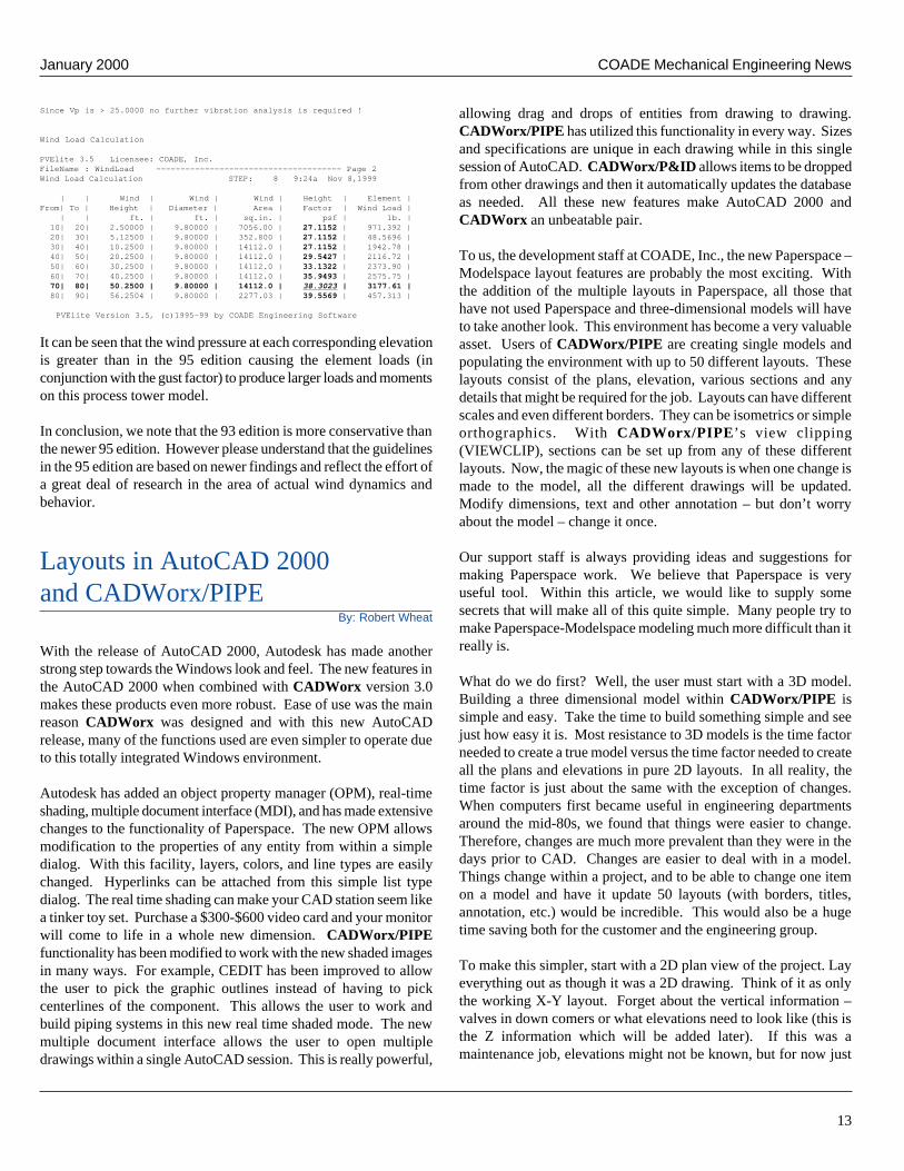
It can be seen that the wind pressure at each corresponding elevationis greater than in the 95 edition causing the element loads (inconjunction with the gust factor) to produce larger loads and momentson this process tower model.

In conclusion, we note that the 93 edition is more conservative thanthe newer 95 edition. However please understand that the guidelinesin the 95 edition are based on newer findings and reflect the effort ofa great deal of research in the area of actual wind dynamics andbehavior.

Layouts in AutoCAD 2000and CADWorx/PIPE

By: Robert Wheat

With the release of AutoCAD 2000, Autodesk has made anotherstrong step towards the Windows look and feel. The new features inthe AutoCAD 2000 when combined with CADWorx version 3.0makes these products even more robust. Ease of use was the mainreason CADWorx was designed and with this new AutoCADrelease, many of the functions used are even simpler to operate dueto this totally integrated Windows environment.

Autodesk has added an object property manager (OPM), real-timeshading, multiple document interface (MDI), and has made extensivechanges to the functionality of Paperspace. The new OPM allowsmodification to the properties of any entity from within a simpledialog. With this facility, layers, colors, and line types are easilychanged. Hyperlinks can be attached from this simple list typedialog. The real time shading can make your CAD station seem likea tinker toy set. Purchase a $300-$600 video card and your monitorwill come to life in a whole new dimension. CADWorx/PIPEfunctionality has been modified to work with the new shaded imagesin many ways. For example, CEDIT has been improved to allowthe user to pick the graphic outlines instead of having to pickcenterlines of the component. This allows the user to work andbuild piping systems in this new real time shaded mode. The newmultiple document interface allows the user to open multipledrawings within a single AutoCAD session. This is really powerful,

allowing drag and drops of entities from drawing to drawing.CADWorx/PIPE has utilized this functionality in every way. Sizesand specifications are unique in each drawing while in this singlesession of AutoCAD. CADWorx/P&ID allows items to be droppedfrom other drawings and then it automatically updates the databaseas needed. All these new features make AutoCAD 2000 andCADWorx an unbeatable pair.

To us, the development staff at COADE, Inc., the new Paperspace –Modelspace layout features are probably the most exciting. Withthe addition of the multiple layouts in Paperspace, all those thathave not used Paperspace and three-dimensional models will haveto take another look. This environment has become a very valuableasset. Users of CADWorx/PIPE are creating single models andpopulating the environment with up to 50 different layouts. Theselayouts consist of the plans, elevation, various sections and anydetails that might be required for the job. Layouts can have differentscales and even different borders. They can be isometrics or simpleorthographics. With CADWorx/PIPE ’s view clipping(VIEWCLIP), sections can be set up from any of these differentlayouts. Now, the magic of these new layouts is when one change ismade to the model, all the different drawings will be updated.Modify dimensions, text and other annotation – but don’t worryabout the model – change it once.

Our support staff is always providing ideas and suggestions formaking Paperspace work. We believe that Paperspace is veryuseful tool. Within this article, we would like to supply somesecrets that will make all of this quite simple. Many people try tomake Paperspace-Modelspace modeling much more difficult than itreally is.

What do we do first? Well, the user must start with a 3D model.Building a three dimensional model within CADWorx/PIPE issimple and easy. Take the time to build something simple and seejust how easy it is. Most resistance to 3D models is the time factorneeded to create a true model versus the time factor needed to createall the plans and elevations in pure 2D layouts. In all reality, thetime factor is just about the same with the exception of changes.When computers first became useful in engineering departmentsaround the mid-80s, we found that things were easier to change.Therefore, changes are much more prevalent than they were in thedays prior to CAD. Changes are easier to deal with in a model.Things change within a project, and to be able to change one itemon a model and have it update 50 layouts (with borders, titles,annotation, etc.) would be incredible. This would also be a hugetime saving both for the customer and the engineering group.

To make this simpler, start with a 2D plan view of the project. Layeverything out as though it was a 2D drawing. Think of it as onlythe working X-Y layout. Forget about the vertical information –valves in down comers or what elevations need to look like (this isthe Z information which will be added later). If this was amaintenance job, elevations might not be known, but for now just


14

draw the piping flat on the piece of paper. Most new jobs willrequire the designer to set elevations based on some type of intelligentdecision after the job becomes more organized. But this is not doneat the beginning of the job. We can apply elevations to the pipinganytime in a very simple manner with the CHANGEELEV commandwithin CADWorx/PIPE. Use the 2D drawing capabilities ofCADWorx/PIPE and create a 2D drawing.

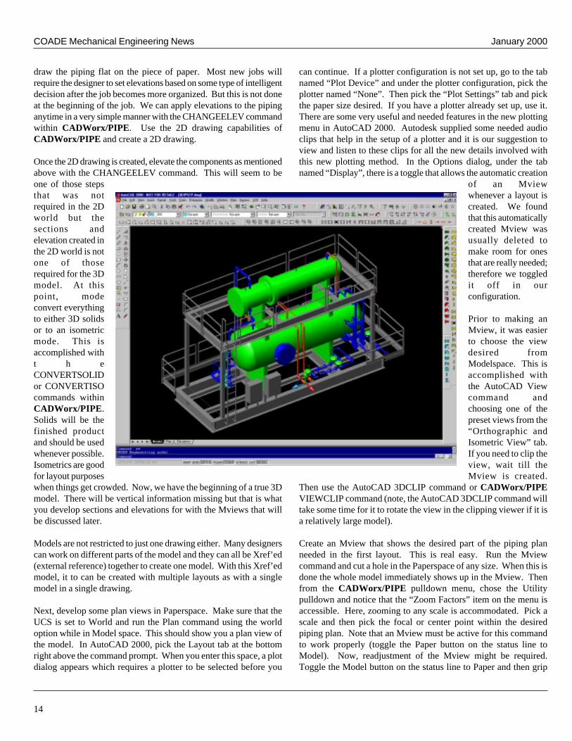
Once the 2D drawing is created, elevate the components as mentionedabove with the CHANGEELEV command. This will seem to beone of those stepsthat was notrequired in the 2Dworld but thesections andelevation created inthe 2D world is notone of thoserequired for the 3Dmodel. At thispoint, modeconvert everythingto either 3D solidsor to an isometricmode. This isaccomplished witht h eCONVERTSOLIDor CONVERTISOcommands withinCADWorx/PIPE.Solids will be thefinished productand should be usedwhenever possible.Isometrics are goodfor layout purposeswhen things get crowded. Now, we have the beginning of a true 3Dmodel. There will be vertical information missing but that is whatyou develop sections and elevations for with the Mviews that willbe discussed later.

Models are not restricted to just one drawing either. Many designerscan work on different parts of the model and they can all be Xref’ed(external reference) together to create one model. With this Xref’edmodel, it to can be created with multiple layouts as with a singlemodel in a single drawing.

Next, develop some plan views in Paperspace. Make sure that theUCS is set to World and run the Plan command using the worldoption while in Model space. This should show you a plan view ofthe model. In AutoCAD 2000, pick the Layout tab at the bottomright above the command prompt. When you enter this space, a plotdialog appears which requires a plotter to be selected before you

can continue. If a plotter configuration is not set up, go to the tabnamed “Plot Device” and under the plotter configuration, pick theplotter named “None”. Then pick the “Plot Settings” tab and pickthe paper size desired. If you have a plotter already set up, use it.There are some very useful and needed features in the new plottingmenu in AutoCAD 2000. Autodesk supplied some needed audioclips that help in the setup of a plotter and it is our suggestion toview and listen to these clips for all the new details involved withthis new plotting method. In the Options dialog, under the tabnamed “Display”, there is a toggle that allows the automatic creation

of an Mviewwhenever a layout iscreated. We foundthat this automaticallycreated Mview wasusually deleted tomake room for onesthat are really needed;therefore we toggledit off in ourconfiguration.

Prior to making anMview, it was easierto choose the viewdesired fromModelspace. This isaccomplished withthe AutoCAD Viewcommand andchoosing one of thepreset views from the“Orthographic andIsometric View” tab.If you need to clip theview, wait till theMview is created.

Then use the AutoCAD 3DCLIP command or CADWorx/PIPEVIEWCLIP command (note, the AutoCAD 3DCLIP command willtake some time for it to rotate the view in the clipping viewer if it isa relatively large model).

Create an Mview that shows the desired part of the piping planneeded in the first layout. This is real easy. Run the Mviewcommand and cut a hole in the Paperspace of any size. When this isdone the whole model immediately shows up in the Mview. Thenfrom the CADWorx/PIPE pulldown menu, chose the Utilitypulldown and notice that the “Zoom Factors” item on the menu isaccessible. Here, zooming to any scale is accommodated. Pick ascale and then pick the focal or center point within the desiredpiping plan. Note that an Mview must be active for this commandto work properly (toggle the Paper button on the status line toModel). Now, readjustment of the Mview might be required.Toggle the Model button on the status line to Paper and then grip


15

the Mview (the hole in the paper) and stretch it as required. Thishole in the paper (Mview) is just like another AutoCAD entity. Thelayer can be changed and it can be turned off in the Layer dialog(move it or create it on the VIEWL layer – this is the purpose of thislayer).

Use the SETUP command within CADWorx/PIPE for setting up aborder. Run the setup command and then chose the Border buttonon the main dialog. Here options are available for placing theborder in Paperspace and choosing the correct border. As withmost of CADWorx/PIPE, customizingthe borders or addinga new border isalways possible.

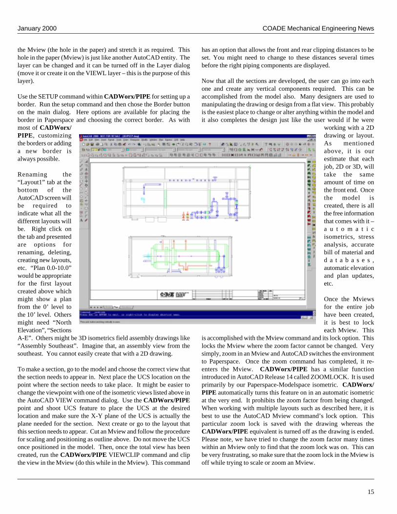
Renaming the“Layout1” tab at thebottom of theAutoCAD screen willbe required toindicate what all thedifferent layouts willbe. Right click onthe tab and presentedare options forrenaming, deleting,creating new layouts,etc. “Plan 0.0-10.0”would be appropriatefor the first layoutcreated above whichmight show a planfrom the 0’ level tothe 10’ level. Othersmight need “NorthElevation”, “SectionsA-E”. Others might be 3D isometrics field assembly drawings like“Assembly Southeast”. Imagine that, an assembly view from thesoutheast. You cannot easily create that with a 2D drawing.

To make a section, go to the model and choose the correct view thatthe section needs to appear in. Next place the UCS location on thepoint where the section needs to take place. It might be easier tochange the viewpoint with one of the isometric views listed above inthe AutoCAD VIEW command dialog. Use the CADWorx/PIPEpoint and shoot UCS feature to place the UCS at the desiredlocation and make sure the X-Y plane of the UCS is actually theplane needed for the section. Next create or go to the layout thatthis section needs to appear. Cut an Mview and follow the procedurefor scaling and positioning as outline above. Do not move the UCSonce positioned in the model. Then, once the total view has beencreated, run the CADWorx/PIPE VIEWCLIP command and clipthe view in the Mview (do this while in the Mview). This command

has an option that allows the front and rear clipping distances to beset. You might need to change to these distances several timesbefore the right piping components are displayed.

Now that all the sections are developed, the user can go into eachone and create any vertical components required. This can beaccomplished from the model also. Many designers are used tomanipulating the drawing or design from a flat view. This probablyis the easiest place to change or alter anything within the model andit also completes the design just like the user would if he were

working with a 2Ddrawing or layout.As mentionedabove, it is ourestimate that eachjob, 2D or 3D, willtake the sameamount of time onthe front end. Oncethe model iscreated, there is allthe free informationthat comes with it –a u t o m a t i cisometrics, stressanalysis, accuratebill of material andd a t a b a s e s ,automatic elevationand plan updates,etc.

Once the Mviewsfor the entire jobhave been created,it is best to lockeach Mview. This

is accomplished with the Mview command and its lock option. Thislocks the Mview where the zoom factor cannot be changed. Verysimply, zoom in an Mview and AutoCAD switches the environmentto Paperspace. Once the zoom command has completed, it re-enters the Mview. CADWorx/PIPE has a similar functionintroduced in AutoCAD Release 14 called ZOOMLOCK. It is usedprimarily by our Paperspace-Modelspace isometric. CADWorx/PIPE automatically turns this feature on in an automatic isometricat the very end. It prohibits the zoom factor from being changed.When working with multiple layouts such as described here, it isbest to use the AutoCAD Mview command’s lock option. Thisparticular zoom lock is saved with the drawing whereas theCADWorx/PIPE equivalent is turned off as the drawing is ended.Please note, we have tried to change the zoom factor many timeswithin an Mview only to find that the zoom lock was on. This canbe very frustrating, so make sure that the zoom lock in the Mview isoff while trying to scale or zoom an Mview.


16

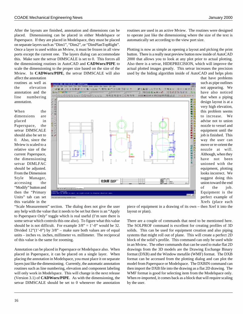
After the layouts are finished, annotation and dimensions can beplaced. Dimensioning can be placed in either Modelspace orPaperspace. If they are placed in Modelspace, they must be placedon separate layers such as “Dim1”, “Dim2”, or “DimPlanTopRight”.Once a layer is used within an Mview, it must be frozen in all viewports except the current one. The layers dialog can accommodatethis. Make sure the setvar DIMSCALE is set to 0. This forces allthe dimensioning routines in AutoCAD and CADWorx/PIPE toscale the dimensioning to the proper size based on the size of theMview. In CADWorx/PIPE, the setvar DIMSCALE will alsoaffect the annotationroutines as well asthe elevationannotation and theline numberingannotation.

When thedimensions areplaced inPaperspace, thesetvar DIMSCALEshould also be set to0. Also, since theMview is scaled to arelative size of thecurrent Paperspace,the dimensioningsetvar DIMLFACshould be adjusted.From the DimensionStyle Manager,accessing the“Modify” button andthen the “PrimaryUnits” tab can setthis variable in the“Scale Measurement” section. The dialog does not give the userany help with the value that it needs to be set but there is an “Applyto Paperspace Only” toggle which is real useful (I’m sure there issome setvar which controls this one also). To figure what this valueshould be is not difficult. For example 3/8” = 1’-0” would be 32.Divided 12”(1’-0”) by 3/8” – make sure both values are of equalunits – inches vs. inches, millimeter vs. millimeter. The reciprocalof this value is the same for zooming.

Annotation can be placed in Paperspace or Modelspace also. Whenplaced in Paperspace, it can be placed on a single layer. Whenplacing the annotation in Modelspace, you must place it on separatelayers just like the dimensioning. Currently, the automatic annotationroutines such as line numbering, elevation and component labelingwill only work in Modelspace. This will change in the next release(Version 3.1) of CADWorx/PIPE. As with the dimensioning, thesetvar DIMSCALE should be set to 0 whenever the annotation

routines are used in an active Mview. The routines were designedto operate just like the dimensioning where the size of the text isautomatically set according to the view port size.

Plotting is now as simple as opening a layout and picking the printbutton. There is a really neat preview button now inside of AutoCAD2000 that allows you to look at any plot prior to actual plotting.Also there is a setvar, HIDEPRECISION, which will improve theactual plotted images greatly. This setvar increases the precisionused by the hiding algorithm inside of AutoCAD and helps plots

that have problemssuch as pipe outlinesnot appearing. Wehave also noticedthat when a pipingdesign layout is at avery high elevation,this problem seemsto increase. Weadvise not to unionnozzle to vessel andequipment until thejob is finished. Thisway the user canmove or re-orient thenozzle at will.Although, when theyhave not beenunioned with theequipment, plottinglooks incorrect. Wesuggest doing thisunion toward the endof the job.Equipment is theperfect example ofXrefs (place each

piece of equipment in a drawing of its own – then Xref it into thelayout or plan).

There are a couple of commands that need to be mentioned here.The SOLPROF command is excellent for creating profiles of 3Dsolids. This can be used for equipment creation and also pipingsystems that might roll out of plane. This will create a perfect 2Dblock of the solid’s profile. This command can only be used whilein an Mview. The other commands that can be used to make flat 2Ddrawings from the 3D models are the Drawing Exchange Binaryformat (DXB) and the Window metafile (WMF) format. The DXBformat can be accessed from the plotting dialog and can plot themodel from Paperspace or Modelspace. The DXBIN command canthen import the DXB file into the drawing as a flat 2D drawing. TheWMF format is good for selecting item from the Modelspace only.When re-imported, it comes back as a block that will require scalingby the user.


17

There are some issues with this method of 3D modeling that are alittle aggravating. There are some things that don’t work or appearcorrectly according to the standards we used to produce 2D drawings.Ball and globe valves don’t appear correctly. Centerlines disappearinto the solid of a component. There is not a good way of breakinga pipe over another system with pipe breaks as we did in a 2Denvironment. But there are ways around these problems. Theproblem with ball and globe valves is they both look the same.However, you can place a circle in Paperspace over the globe valvethen place a solid hatch within the circle. Breaking pipe overanother system might not be needed since that system below can beclipped out and shown somewhere else. It’s not like having toredraw it. It’s all part of the model. The centerline problem is onethat we don’t have a solution for. Losing centerlines versus gettinga model that automatically updates all the drawings would be wellworth it to me.

The next generation of CADWorx/PIPE will handle the problemsas mentioned above. The components in our next generation systemwill allow centerline viewing. Breaking will be allowed on pipetype components and globe valve when viewed in a plan or elevationwill appear as they have for the last 100 years. When the view ischanged back to 3D, things will look as they are in our presentCADWorx/PIPE. Hopefully completed within the next year, thissystem will truly leap beyond the traditional 2D drafting techniquesand give us a tool where there will be no comparison.

PC Hardware/Software for theEngineering User [Part 28]

By: Richard Ay

Q: How can I improve I/O performance?

A: If your system is fairly I/O intensive, you may benefit from raisingthe I/O Page Lock Limit, which can increase the effective rate theoperating system reads or writes data to the hard disks.

First, benchmark your common tasks. See how long it takes to loadand save large files, how long it takes to search a database or run acommon program; just do your normal tasks, timing them to recordhow fast they are. Then follow these steps:

1. Start the registry editor (regedit.exe)

2. Move to HKEY_LOCAL_MACHINE\SYSTEM\CurrentControlSet\Control\Session Manager\MemoryManagement

3. Double click IoPageLockLimit

4. Enter a new value.

This value is the maximum bytes you can lock for I/Ooperations. A value of 0 defaults to 512KB. Raise this valueby 512KB increments (enter “512”, “1024”, etc.), then exitregedit and benchmark your system after each adjustment.When an increase does not give you a significant performanceboost, go back and undo the last increment.

Caution: There is a limit to this. Do not set this value (inbytes) beyond the number of megabytes of RAM times 128.That is, if you have 16 MB RAM, do not set IoPageLockLimitover 2048 bytes; for 32MB RAM, do not exceed 4096bytes, and so on.

5. Click OK.

6. Close the registry editor

Unless you do little I/O, this should give you a significant boost inperformance.

Q: My machine has a “constant” connection to the internet. Is mymachine secure?

A: Check out the link http://www.grc.com/, which will load a webpage designed to test the security of your computer. (Click on the“ShieldsUp” icon.) This web site contains all the details you needto check out the security of your system, including explanations ofsecurity details. A related article can be found on Ziff Davis’s siteat http://cgi.zdnet.com/slink?10862:1590013

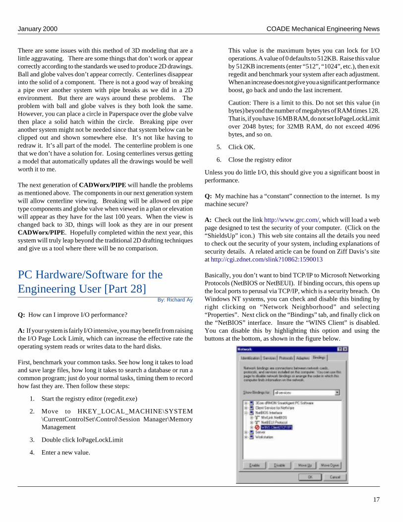
Basically, you don’t want to bind TCP/IP to Microsoft NetworkingProtocols (NetBIOS or NetBEUI). If binding occurs, this opens upthe local ports to perusal via TCP/IP, which is a security breach. OnWindows NT systems, you can check and disable this binding byright clicking on “Network Neighborhood” and selecting“Properties”. Next click on the “Bindings” tab, and finally click onthe “NetBIOS” interface. Insure the “WINS Client” is disabled.You can disable this by highlighting this option and using thebuttons at the bottom, as shown in the figure below.


18

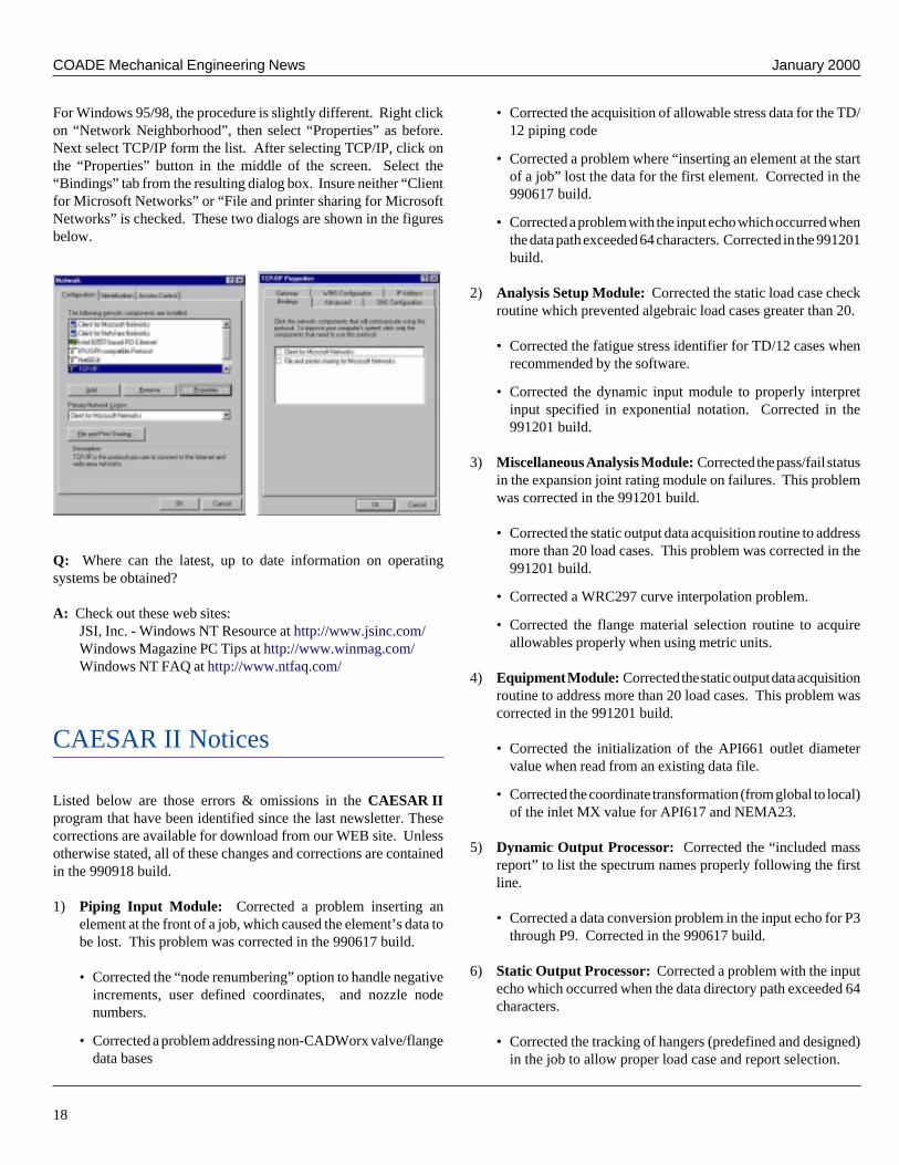
For Windows 95/98, the procedure is slightly different. Right clickon “Network Neighborhood”, then select “Properties” as before.Next select TCP/IP form the list. After selecting TCP/IP, click onthe “Properties” button in the middle of the screen. Select the“Bindings” tab from the resulting dialog box. Insure neither “Clientfor Microsoft Networks” or “File and printer sharing for MicrosoftNetworks” is checked. These two dialogs are shown in the figuresbelow.

Q: Where can the latest, up to date information on operatingsystems be obtained?

A: Check out these web sites:JSI, Inc. - Windows NT Resource at http://www.jsinc.com/Windows Magazine PC Tips at http://www.winmag.com/Windows NT FAQ at http://www.ntfaq.com/

CAESAR II Notices

Listed below are those errors & omissions in the CAESAR IIprogram that have been identified since the last newsletter. Thesecorrections are available for download from our WEB site. Unlessotherwise stated, all of these changes and corrections are containedin the 990918 build.

1) Piping Input Module: Corrected a problem inserting anelement at the front of a job, which caused the element’s data tobe lost. This problem was corrected in the 990617 build.

• Corrected the “node renumbering” option to handle negativeincrements, user defined coordinates, and nozzle nodenumbers.

• Corrected a problem addressing non-CADWorx valve/flangedata bases

• Corrected the acquisition of allowable stress data for the TD/12 piping code

• Corrected a problem where “inserting an element at the startof a job” lost the data for the first element. Corrected in the990617 build.

• Corrected a problem with the input echo which occurred whenthe data path exceeded 64 characters. Corrected in the 991201build.

2) Analysis Setup Module: Corrected the static load case checkroutine which prevented algebraic load cases greater than 20.

• Corrected the fatigue stress identifier for TD/12 cases whenrecommended by the software.

• Corrected the dynamic input module to properly interpretinput specified in exponential notation. Corrected in the991201 build.

3) Miscellaneous Analysis Module: Corrected the pass/fail statusin the expansion joint rating module on failures. This problemwas corrected in the 991201 build.

• Corrected the static output data acquisition routine to addressmore than 20 load cases. This problem was corrected in the991201 build.

• Corrected a WRC297 curve interpolation problem.

• Corrected the flange material selection routine to acquireallowables properly when using metric units.

4) Equipment Module: Corrected the static output data acquisitionroutine to address more than 20 load cases. This problem wascorrected in the 991201 build.

• Corrected the initialization of the API661 outlet diametervalue when read from an existing data file.

• Corrected the coordinate transformation (from global to local)of the inlet MX value for API617 and NEMA23.

5) Dynamic Output Processor: Corrected the “included massreport” to list the spectrum names properly following the firstline.

• Corrected a data conversion problem in the input echo for P3through P9. Corrected in the 990617 build.

6) Static Output Processor: Corrected a problem with the inputecho which occurred when the data directory path exceeded 64characters.

• Corrected the tracking of hangers (predefined and designed)in the job to allow proper load case and report selection.


19

• Corrected a data conversion problem in the input echo for P3through P9. Corrected in the 990617 build.

7) Material Data Base Editor: Corrected a problem when editinguser materials which caused the material to be added again,instead of modified.

8) Piping Error Checker: Corrected the allowable stressacquisition routine to handle the case where a user checked the“allowable stress check box”, but didn’t enter any data. Correctedin the 991201 build.

• Corrected the acquisition of allowable stress data for the TD/12 piping code.

• Corrected an error which copied force vector #7 into vectors#8 and #9. Corrected in the 990617 build.

• Modified necessary TD/12 calculations as per Transco'svalidation project. Corrected in the 991201 build.

9) Dynamic Stress Computation Module: Corrected an errorprocessing the cyclic reduction factors to temperatures 4 through9 when determining the allowable dynamic stress. Corrected inthe 990617 build.


10) Static Stress Computation Module: Corrected the computationof the allowable stress for the Z662 code, for the “from” end ofelements in tension. Corrected in the 990617 build.


11) Element Generator: Modified Bourdon Pressure calculations.Corrected in the 991201 build.

TANK Notices

Listed below are those errors & omissions in the TANK programthat have been identified since the last newsletter. These correctionsare available for download from our WEB site. Unless otherwisestated, all of these changes and corrections are contained in the990811 build.

1) Input Module: Corrected the acquisition of stainless steelallowables from the material data base when using non-Englishunits.

• Corrected the units conversion constant for the girder ringradius.

• Corrected several resource ID values which caused incorrecttext labels on some dialog boxes. Corrected in the 991005build.

• Corrected the shell course material input so users can changematerials once the job is defined. Corrected in the 991005build.

2) Error Check Module: Corrected the units conversion constantfor the girder ring radius.

3) Solution Module: Corrected a variable misspelling whichcaused the value of “maximum pressure limited by uplift ininches of H2O” to be reported as zero.

4) Output Module: Corrected a variable misspelling whichcaused the number of user defined anchor bolts to be reported aszero.

CODECALC Notices

Listed below are those errors & omissions in the CODECALCprogram that have been identified since the last newsletter. Thesecorrections are available for download from our WEB site.

1) In WRC 297, there were a few unit conversion problems in theresults and an import function units conversion error when theunits were not English. Also a curve interpolation problem wascorrected. Also a check box for the use of ASME Section VIIIDivision 2 stress indices was added. To maintain compatibilitywith previous results, this box must be checked. The defaultsetting is not checked.

2) For the ASME fixed tubesheet, the factor J was not properlycomputed when there was no expansion joint. This was anunconservative error. This problem has been resolved.

3) Some other fixes/enhancements were made to the U-tube requiredthickness calculation when the elastic/plastic iteration was beingperformed.

4) In the flange routine, circular blind flanges were being treated asnon-circular resulting in a higher than required thickness.

5) The conical discontinuity stress calculations were slightlymodified. The new results may vary slightly with the previousresults, depending on the input and the magnitude of the forceson the top and bottom of the cone.


20

6) Small nozzles on flat heads were being computed regardless ofhow small the finished opening was.

7) In the shell and head module the minimum thickness has been setto 1/16 of an inch. Additionally, some other cosmetic changeswere made to the printout.

8) The merge button in the ASME tubesheet, Tema Tubesheet andhorizontal vessel was not properly accounting for the diameterbasis.

9) In the rectangular vessel program, the Membrane stress MAWPfor figure A3 was in error and has been corrected.

PVElite Notices

Listed below are those errors & omissions in the PVElite programthat have been identified since the last newsletter. These correctionsare available for download from our web site.

1) The vortex shedding routines were obtaining results that wereextremely conservative due to a units conversion error. Thisproblem has been corrected.

2) The conical discontinuity stress calculations were slightlymodified. The new results may vary slightly with the previousresults, depending on the input and the magnitude of the forcesand moments on the top and bottom of the cone.

3) The BS-5500 head thickness routine failed to obtain the correctresult in one known case. The routine was re-written to solve theproblem. Also the MAWP computation for heads was reworkedat the same time and now gives correct results. This problemoccurred on elliptical and torispherical heads. Also, some of thenomenclature was updated in the BS-5500 nozzle analysis andsome conservative error checks were resolved.

4) There was an error in the CodeCase 2260/2261 calculations forsome geometries that caused the thickness to be more conservativethan the regular ASME equations.

5) The thickness limit for hub type nozzles using Division 1 wasconservative in some cases. This problem has been fixed.

12777 Jones Rd. Suite 480 Tel: 281-890-4566 Web: www.coade.comHouston, Texas 77070 Fax: 281-890-3301 E-Mail: [email protected]

COADE Engineering Software

mechanical engineering news - plantdesignsolutions...coade mechanical engineering news january 2000...

Documents