Mecro-Economic Voting:Local Information and Micro-Perceptions of the

Macro-Economy∗

Stephen Ansolabehere Marc Meredith Erik SnowbergHarvard University University of California Institute

Pennsylvania Technologysda@gov.harvard.edu marcmere@sas.upenn.edu snowberg@caltech.edu

November 29, 2010

Abstract

We confront a central assertion of the Kramer (1983) critique of using survey data tostudy economic voting: namely, that individuals’ reported economic perceptions con-tain information that is largely unrelated to the economy. We show theoretically thatindividuals who are trying to understand their own economic situation will often bebetter off relying on local—rather than personal or national—economic information,and that this produces behavior similar to sociotropic voting. Examining data from anovel survey instrument that asks respondents their numerical assessment of the unem-ployment rate confirms this hypothesis. Specifically, individuals’ economic perceptionsrespond to local conditions. Moreover, these perceptions associate with individuals’vote choices. Extending our analysis to a time series of polls from 1980–2008, we ver-ify that patterns in individual data also exist in aggregate economic perceptions andpolitical support.

∗We thank Mike Alvarez, Conor Dowling, Ray Duch, Jon Eguia, Nolan McCarty, Stephanie Rickard, KenScheve, and Chris Wlezien for encouragement and suggestions, and seminar audiences at LSE, MIT, NYU,Temple and Yale for useful feedback and comments.

1 Introduction

One of the most robust relationships in political economy is economic voting: the positive

correlation between an area’s economic performance and the political performance of incum-

bent politicians and parties.1 Motivated by this aggregate pattern, scholars have developed

many theories about how the economy influences individuals’ vote choices. While all theo-

ries of economic voting require individuals to make economic assessments that inform vote

choice, they differ in terms of how assessments are made and used. For example, egotropic,

or pocketbook, theories posit that individuals vote based on assessments of their own eco-

nomic circumstances, while sociotropic theories posit that individuals vote based on their

assessment of national economic conditions (Kinder and Kiewiet, 1979, 1981; Kiewiet, 1983).

Discriminating between different theories of economic voting using aggregate data is

difficult, as most theories produce the same aggregate predictions.2 Thus, many scholars

turn to cross-sectional survey data.

However, Kramer (1983) and others critique the use of cross-sectional variation in percep-

tions of the national economy to identify the effect of the national economy on vote choice.

As summarized by Lewis-Beck and Paldam (2000, pp. 195–196), “Kramer’s (1983) standing

dissent [is] that in a survey cross-section there can be no ‘real’ variance because there is only

one economy being measured at one point in time.” That is, most of the cross-sectional

variation in economic perceptions is driven by extraneous factors.

Contrary to Kramer, we argue that cross-sectional variation in voters’ economic percep-

tions reflects real differences in local conditions. Our argument starts with Downs’s (1957)

and Popkin’s (1991) observation that voters have little incentive to expend costly effort

gathering information to make political decisions. Rather, individuals gather economic in-

formation to inform personal economic choices, and use the same information to inform their

1The literature on economic voting is truly massive. For recent reviews of the literature see Lewis-Beckand Paldam (2000) and Hibbs (2006).

2At the aggregate level, most studies focus on the relationship between national measures of economicperformance, such as economic growth, unemployment, or inflation, and the vote share or approval rating ofthe incumbent party (Kramer, 1971; Fair, 1978; Lewis-Beck, 1988).

1

political choices. Thus, individuals will gather information that will generally provide only

an imperfect understanding of aggregate (national) economic conditions. More precisely, in-

formation about local economic conditions is the most informative for economic choices, and

the easiest to gather through family, friends, neighbors and professional networks. More-

over, this information will generally not be sufficient to precisely infer national economic

conditions.

We use our theory of local information acquisition to generate predictions about the cross-

sectional variation in economic perceptions. Individuals are members of groups—based on

characteristics such as age, race, educational level, and location of residence—that experience

different economic conditions. Following some economists, we refer to these groups as an

individual’s mecro-economy (so-called because it is in somewhere between the macro- and

micro-economy). As information about economic conditions in individuals’ mecro-economies

is freely available and useful for economic planning, we predict that individuals’ economic

perceptions will differ based on demographic factors correlated with economic well-being. For

example, because unemployment decreases with education, we predict that perceptions of the

unemployment rate will also decrease with education. Additionally, we predict individuals’

perceptions of the aggregate economy will be influenced by economic conditions in their

locality; that is, perceptions of the aggregate economy will be worse in localities where

the economy is performing relatively poorly and better in localities where the economy is

performing relatively well. Moreover, we predict that political support will be influenced by

these economic perceptions, and thus by mecro-economic conditions.

We investigate these predictions using a novel survey instrument from the 2008 Coop-

erative Congressional Election Survey (CCES) that asks respondents to give a numerical

assessment of the unemployment rate. We focus throughout on unemployment because it is

important for economic voting, is directly experienced by individuals, and varies markedly,

and measurably, between groups. Unemployment has been found to have an independent

bearing on election outcomes, although, at an aggregate level, economic growth is thought

2

to be a more important correlate of the economic vote (Kramer, 1971; Fair, 1978; Duch and

Stevenson, 2008). Further, employment and unemployment are directly experienced by in-

dividuals, their friends, and their neighbors. Indeed, it is likely easier to observe whether or

not your neighbor is employed—which is informative of unemployment—than it is to gauge

the size of a raise he or she may or may not have gotten—which is informative of economic

growth. Finally, unlike economic growth, unemployment is often tabulated by demographic

group, allowing us to test whether groups that report higher perceptions of the unemploy-

ment rate do, in fact, experience higher rates of unemployment. For similar reasons we focus

on numerical reports of unemployment perceptions: they are easier to compare with real

world figures and easier to incorporate into theory.3

In accordance with theory, we find that individuals who are employed, but more likely to

be unemployed, report higher national unemployment rates. Specifically, women, African-

Americans, low-income workers and respondents from states with higher unemployment rates

all report higher rates of unemployment. Moreover, perceptions of unemployment rates are

correlated with vote choice, even when controlling for numerous other factors.

To generalize these findings, we investigate the extent to which local unemployment rates

relate to economic assessments and presidential support using state-level data from 1980 to

2008. This allows us to verify our argument in aggregate, time-series data—the type of data

endorsed by Kramer. We find a robust significant relationship between the unemployment

rate in a state and responses to the standard retrospective economic question asked as part

of the American National Election Study (ANES). Moreover, variations around national

trends in state-level unemployment rates are robustly correlated with state-level presidential

approval as measured by Gallup. Thus, the patterns observed in cross-sectional data are

informative of patterns in aggregate data over time.

3This follows Alvarez and Brehm (2002) in focusing on hard information when assessing the informationsets of respondents, which may better isolate variation in reported economic evaluations that are rootedin differences in actual economic perceptions (Ansolabehere, Meredith and Snowberg, 2011). For more onthe advantages and design of survey questions that ask about numbers, see Ansolabehere, Meredith andSnowberg (2010).

3

1.1 Responses to Kramer’s Critique

There have been two divergent responses to Kramer’s (1983) critique. Many scholars ignore

Kramer’s advice and continue to relate cross-sectional variation in respondents’ economic

perceptions and political support (Lewis-Beck, 1988; Duch and Stevenson, 2008). The most

common form of individual-level data on national economic perceptions comes from the stan-

dard retrospective economic evaluation—a survey question that asks respondents whether

the national economy is better, worse, or about the same as a year ago. Such data exhibits

cross-sectional variation in national economic perceptions that is robustly associated with

support for the incumbent’s party.

Kramer’s critique is often invoked when questioning the validity of this approach. Van

der Brug, van der Eijk and Franklin (2007, pp. 195–196) goes as far as to conclude that,

“Studies estimating the effects of subjective evaluations cannot be taken seriously as proper

estimates of the effects of economic conditions.” Recent research has particularly focused

on the problem of reverse causality; that is, that some of the cross-sectional variation in

individual’s economic perceptions is caused by their political support (Wlezien, Franklin

and Twiggs, 1997; Anderson, Mendes and Tverdova, 2004; Evans and Andersen, 2006).

The second response is to abandon individual-level data and, instead, relate time-series

variation in aggregate economic measures to time-series variation in aggregate political sup-

port. These economic measures can either be aggregated subjective economic evaluations

(e.g. MacKuen, Erikson and Stimson, 1992; Erikson, MacKuen and Stimson, 2002) or objec-

tive measures of economic performance like economic growth or the unemployment rate (e.g.

van der Brug, van der Eijk and Franklin, 2007). By ignoring the cross-sectional variation in

economic perceptions, these studies limit their susceptibility to bias from reverse causality.

As a result, it is not surprising that the associations between economic conditions and vote

choice identified using time series variation tend to be smaller than those identified using

cross-sectional variation (Duch and Armstrong, 2010).

Treating the economy as a monolithic entity at a given point in time, however, is not

4

without cost. Aggregating economic evaluations eliminates actual differences in individuals’

economic perceptions that may affect political support. That is, in the same election, in-

formational differences may lead some individuals to support the incumbent because they

perceive the economy is performing well, while others may support the challenger because

they perceive the economy is performing poorly.4 Consequently, aggregation may result in re-

searchers underestimating the degree of economic voting.5 Moreover, this approach obscures

the specific mechanisms of economic voting.

2 Theory

Our theory is composed of two related aspects. The first is the observation that the economy

is not monolithic: there are different sectors of the economy, and different professions within

a given sector that may have different fortunes over the same time period. For example, a

particular year may see large growth in the accounting industry and a precipitous decline in

agricultural prices, and thus farmers’ fortunes. Moreover, within auto manufacturing, it may

be the case that economic policies and conditions favor increased automation that leads to

higher profits and salaries for managers, but layoffs for workers. These trends are somewhere

between the micro- and the macro-economy, a space economists sometimes refer to as the

mecro-economy.

The second aspect is that individuals attempt to understand the effect different politi-

cians have on their economic outcomes, and vote on the basis of this understanding. While

there are many mechanisms that might lead to similar outcomes, we adopt a particularly

simple formulation. Specifically, in the process of economic planning individuals also ob-

tain information on the effect of the incumbents’ policies. This information causes them

4The results in Hetherington (1996) suggest that such behavior may have occurred in the 1992 presidentialelection. See Krause (1997); Anderson, Duch and Palmer (2000) for previous work on heterogeneity ineconomic evaluations.

5For example, suppose that individuals’ economic perceptions are equal to the true state of the economyplus some white noise. In such a case, assuming that everyone has identical economic perceptions implies ran-dom mis-measurement of an explanatory variable, which is well-known to cause attenuation of its estimatedeffect on a dependent variable.

5

to update their beliefs about whether the incumbent’s policies are good or bad for them.

Each individual compares his or her ex-post belief to a common baseline, and votes for the

incumbent if his or her ex-post belief is greater than the baseline, and otherwise he or she

votes for the opposition.

As we argue in the next section, the most useful, and easiest to gather, information for

economic planning is from an individual’s mecro-economy. This, along with the two aspects

above, implies that individuals will have different information, and hence beliefs, about the

state of the economy that will, on average, reflect the situation in an individual’s mecro-

economy. These differing beliefs will lead to different vote choices. Thus, to the extent

that an individual is self-interested, he or she will vote based on mecro-economic conditions.

For example, if members of an individual’s family, neighborhood, and profession all have

jobs, he will conclude that his personal unemployment rate—that is, the probability he will

become unemployed—is low under the incumbent, and vote to retain her. In contrast, if

many members of an individual’s family, neighborhood, and profession are jobless, he will

conclude that his personal unemployment rate is high under the incumbent, and vote for the

opposition.

3 A Prediction: Sociotropic Voting

Here we show that the theory above produces patterns that resemble the empirical regularity

of sociotropic voting: individuals vote largely on the basis of general, rather than personal,

economic conditions. This result may seem counter-intuitive, as mecro-economic voting

centers on the individual’s attempt to understand his or her personal economic circumstances.

However, it follows from the fact that general trends provide more information about an

individual’s personal unemployment rate—that is, the probability of the individual becoming

unemployed—than does the single observation of an individual’s current employment status.

This section sketches an argument made formally in the appendix.

6

Consider an individual who is planning for the next year, and will use information he

gathers in the course of economic planning to inform his vote. Under standard assumptions,

individuals will want to save against the possibility of becoming unemployed in the future.

In order to appropriately save, individuals gather information to estimate their personal

unemployment rate, that is, the probability they will become unemployed the following year.

To the extent that this personal unemployment rate is tied to the incumbent’s economic

policies, this information will also be useful in deciding for whom to vote.

In the tradition of citizen-candidate models (Osborne and Slivinski, 1996; Besley and

Coate, 1997), the policies of both the incumbent and challenger are fixed and known. In

accordance with the findings in Alvarez and Brehm (2002), the effects of those policies on an

individual’s personal unemployment rate are unknown. Thus, current economic information

is useful to an individual trying to infer his personal unemployment rate under the incumbent.

For concreteness, assume that an individual can have a personal unemployment rate that is

either 10% (high) or 5% (low). Suppose further that before a politician is elected, there is

a 50% chance that her economic policies will cause the individual to have a high personal

unemployment rate.

In the model, there are two potential sources of information about an individual’s personal

unemployment rate: his current employment status, and the unemployment rate of people

who are similar to him. However, personal unemployment status is much less informative

than the unemployment rate of people who are similar to him. If an individual is unemployed,

then he will believe there is a 67% chance that the incumbent’s economic policies have

resulted in a high unemployment rate for him. But, if 5% of people that are similar to him

are unemployed, he will be nearly certain that the incumbent’s policies have induced a low

personal unemployment rate, regardless of his current employment status. Moreover, note

that if the individual is employed, there is only a 51% chance that the incumbent’s economic

policies have resulted in a low unemployment rate. Thus, when an individual is employed,

the unemployment rate of people similar to him will be even more valuable.

7

Obviously, if an individual could observe a large number of people who were exactly like

him, he would have a perfect signal of his personal unemployment rate. However, generally

one can only observe a limited number of individuals who are not exactly the same. That

is, he can observe the unemployment rate in his mecro-economy.

How highly correlated must an individual’s mecro-economic and personal unemployment

rate be for the individual to ignore his personal employment status? As shown in the

appendix, these rates must have a correlation greater than 13.

Is it reasonable that the correlation between the individual’s mecro-economic and personal

unemployment rates have a correlation greater than 13? As a proxy, the correlation in annual

unemployment rates between the U.S. average and any state, over the period from 1976 to

2008, is greater than 23

for all states but Wyoming, where the correlation is 0.44. Therefore,

it is likely that any relevant unemployment rate has a sufficiently high correlation to warrant

individuals ignoring their personal employment status.6

The implication of this simple example is quite similar to the empirical regularity referred

to as sociotropic voting—individuals’ reports of general economic trends are more predictive

of vote choice than reports of personal economic circumstances.7 Here, this occurs not

because of altruism, but because group level information is a powerful signal of whether or

not the incumbent’s economic policies are good for the individual.

3.1 From a Mecro-Economy to the Macro-Economy

Our main results, discussed at length in the next section, are concerned with individuals’

perceptions of the national unemployment rate. However, before turning to these results,

we must fill in the step between individuals’ perceptions of their mecro-economy and those

6An individual’s employment status may still be useful information. When a individual cannot directlyobserve unemployment rates, being unemployed is a signal that the individual’s personal unemployment rateis high. As shown in the next section, unemployed individuals do indeed perceive the unemployment rate ishigher.

7It should be noted that the sociotropic hypothesis is largely concerned with voters’ motivations. Here,we assume voters are motivated by personal concerns, but their information differs in ways that is correlatedwith group membership. Kinder, Adams and Gronke (1989) refer to voting based on group-level economicperformance as the “group hypothesis”.

8

of the macro-economy.

Individuals invest in economic information to the extent it increases their own utility. In

the case of unemployment, individuals gather information about others’ employment status

to gain information about their own future income. As shown formally in the appendix,

holding costs equal, individuals prefer signals of the current state of unemployment that

are more directly related to their own probability of future unemployment, as this improves

their economic planning. However, there is a tradeoff between sampling variance and sam-

pling bias. At one extreme is an individual’s own unemployment status, which measures

an individual’s exact quantity of interest—their own probability of being unemployed under

the incumbent—but with a small sample size that results in a large amount of sampling

error. At the other extreme is the national unemployment rate, which is drawn from a large

enough sample to essentially eliminate sampling error, but pools an individual’s personal

unemployment rate of interest with the rates of everyone else.

Thus, an individual prefers information that is somewhere between the national and the

personal level. This information has lower sampling variance than personal information, and

lower sampling bias than national information. Moreover, information about an individual’s

mecro-economy is essentially free. Local information arrises in an individual’s everyday

interactions in his or her home, neighborhood, and workplace.

The assertion that local information arrises as a by-product of everyday interactions

has a testable implication: namely, those with more relevant interactions should have more

accurate assessments of local conditions. We test this implication using data on individuals’

perceptions of gas prices, elicited as part of the 2006 American National Election Study pilot.

Controlling for a host of demographic factors, each extra day per week an individual drove

made his or her perception 7% more accurate than average, and each extra day per week

an individual reported noticing gas prices induced an independent 8% increase in accuracy.8

To put this another way, controlling for other factors, an individual who drove to work and

8This regression contains all of the controls found in Table 1, as well as state fixed effects. Results areavailable from the authors on request.

9

noticed gas prices five days a week would be 75% more accurate than the average respondent.9

As local information is more relevant to economic planning and less costly to gather (Pop-

kin, 1991), we expect most individuals will base their reports of macro-economic conditions

on their perceptions of their mecro-economy. Because local and national conditions are pos-

itively correlated, we expect that individuals observing worse local conditions will perceive

that the national economy is worse. As a result, those observing higher local unemployment

will report higher national unemployment rates. Of course, it is unlikely that no-one in our

sample knows the national unemployment rate. However, to the extent that certain individ-

uals do, this will only attenuate the differences in economic perceptions between groups.10

4 Asking About Unemployment

Our main results, discussed in this section, concern the following question asked of 3000

respondents to the 2008 Cooperative Congressional Election Survey (CCES):

The unemployment rate in the U.S. has varied between 2.5% and 10.8% between

1948 and today. The average unemployment rate during that time was 5.8%.

As far as you know, what is the current rate of unemployment? That is, of the

adults in the US who wanted to work during the second week of October, what

percent of them would you guess were unemployed and looking for a job?

Figure 1 displays the general pattern in the data: groups that experience more unem-

ployment report, on average, higher unemployment rates. This is true whether the average

9Everyday interactions may also affect preferences. Egan and Mullin (2010) find that local weatherconditions affect individuals’ feelings about the importance of policies aimed at curbing global warming.

10The idea that individuals have different costs of learning information is reflected in many public opinionstudies, for example, Alvarez and Franklin (1994); Alvarez (1997); Bartels (1986); Luskin (1987); Zaller(1992); and Zaller and Feldman (1992).

A final question must be addressed here: why not just ask about local unemployment conditions? Aquestion that asked respondents for their perceptions of unemployment among, say, only their gender maylead them to ignore information about unemployment among people of their race. As we are interested inhow all of a respondent’s information shapes his or her perception of the unemployment rate, we have chosento ask for unemployment rates unconditioned on any particular group or location.

10

is measured according to the median or mean. Note that in order to prevent unusually high

responses from driving differences in the mean, we top code responses at 25% throughout.11

While Figure 1 is consistent with the pattern predicted by theory, one might worry

that these perceptions are driven by other factors, such as partisanship. Focusing on age:

perhaps younger people are more liberal, and the more liberal a person is, the higher he

or she perceives unemployment to be. While it is unlikely that we could establish a causal

relationship between a person’s mecro-economic environment and his or her perception of

unemployment rates, we can certainly control for observable correlates in more complete

regression analyses.

Table 1 presents exactly these analyses. The second and fourth columns contain OLS

specifications. The coefficient on any particular attribute can be seen as the difference

between the mean reported unemployment rate for respondents with that attribute and a

baseline, controlling for observable characteristics. Columns 1 and 3 contain a least absolute

difference (LAD) specification, which can be thought of as a median regression. That is,

the coefficient on any particular attribute can be seen as the difference between the median

reported unemployment rate for respondents with that attribute and a baseline, controlling

for observable characteristics. Consistent with Figure 1, the OLS coefficients (difference

between means by group) are greater than the LAD coefficients (difference between medians

by group).

The first pair of specifications in Table 1 differ from the second pair only in how they treat

location. The first two columns contain state fixed effects, consistent with the specification

for all other attributes. In both specifications, these state-by-state dummies are jointly

statistically significant. However, it is possible that this correlation results from respondents

in states with lower unemployment rates reporting higher unemployment rates, contrary to

the predicted patterns. To examine this possibility, the second pair of columns include each

11This affects 6.3% of respondents. Top coding at 15% through 50% (or just dropping observations overthat level) produces qualitatively similar results. In general, the greater the value at which top coding begins,the more pronounced the differences between groups.

11

Figure 1: Reported unemployment rates increase as the true unemployment rate of a groupincreases.

0

2%

4%

6%

8%

10%

12%

Unemployment and Perceptions by Race or Ethnicity

African American Hispanic White, Non−Hispanic

0

2%

4%

6%

8%

10%

12%

Unemployment and Perceptions by Age

Age 18−24 Age 25−44 Age 45−64 Age 65+

0

2%

4%

6%

8%

10%

12%

Unemployment and Perceptions by Education

High School Diploma or Less Some College College Degree or more

Mean Reported Unemployment

Median Reported Unemployment

Group Unemployment, October 2008

Notes: Reported unemployment is top-coded at 25% in order to reduce the influenceof outliers in the means. Means and medians are determined using sampling weights.

12

state’s unemployment rate, rather than state fixed effects, in the regression.12

The coefficients in Table 1 generally agree with the patterns in Figure 1: groups that

experience more unemployment report, on average, higher unemployment rates. This can be

seen by comparing the coefficients in Table 1 with Table 2, which contains unemployment

data from the Bureau of Labor Statistics (BLS) for October, 2008. However, there are two

notable deviations: even though both women and married men had lower unemployment

rates than unmarried men, they perceive higher unemployment rates.

Women may report higher unemployment rates because they participate in the labor

force at a lower rate, as shown in Table 2. In most cases, groups with higher labor force

non-participation are more likely to be unemployed. This is not the case for women. To

the extent that the unemployment rate does not accurately reflect discouraged workers, it

may be that women perceive a higher unemployment rate because their peer group includes

many discouraged workers. While the BLS would view these women as being labor force

non-participants, respondents may classify them as unemployed.13

Despite the fact that the BLS does not provide labor force participation by marital status,

it seems likely that married men have a higher labor force participation rate then unmarried

men. Why then do married men report higher unemployment rates than unmarried men?

A potential answer comes from the literature on international political economy (IPE). IPE

studies show that married men are more likely to favor protectionist trade policies, and

scholars attribute this to married men having more economic anxiety.14 While anxiety

about the economy may lead married men to exaggerate the unemployment rate as well

as the threat of free trade, it seems more appropriate here to simply note that married men

12Including variables that change only at a group level can introduce auto correlation that may biasstandard errors. To correct for this problem, we use robust standard errors clustered at the state level inthe OLS specification, and block bootstraped standard errors for the LAD specification. The block is at thestate level.

13Note that the BLS tracks several alternative measures of unemployment, some of which try to accountfor discouraged and underemployed workers (especially their U-6 measure). Unfortunately, we have notfound these statistics broken down by gender. Moreover, while perceptions of unemployment by occupationwould likely be of great interest, the CCES does not contain data on respondent occupation.

14See, for example, Hiscox (2006). We thank Stephanie Rickard for pointing this out to us.

13

Table 1: Correlates of Reported Unemployment (CCES, N = 2875)

Democrat 0.56∗∗∗ 1.26∗∗∗ 0.54∗∗∗ 1.22∗∗∗

(0.08) (0.22) (0.08) (0.25)

Independent 0.33∗∗∗ 0.84∗∗∗ 0.30∗∗∗ 0.76∗∗∗

(0.07) (0.20) (0.08) (0.18)

Age 18–24 0.90∗∗ 2.45∗∗∗ 0.79∗∗∗ 2.49∗∗∗

(0.41) (0.55) (0.15) (0.55)

Age 25–44 0.52∗∗∗ 1.48∗∗∗ 0.47∗∗∗ 1.47∗∗∗

(0.10) (0.24) (0.09) (0.25)

Age 45–64 0.18∗∗∗ 0.62∗∗∗ 0.18∗∗ 0.63∗∗∗

(0.06) (0.20) (0.08) (0.17)

Married Male 0.23∗∗ 0.53∗∗ 0.18∗ 0.47∗∗∗

(0.10) (0.22) (0.09) (0.16)

Unmarried Female 0.72∗∗∗ 2.26∗∗∗ 0.65∗∗∗ 2.22∗∗∗

(0.16) (0.33) (0.10) (0.37)

Married Female 0.64∗∗∗ 2.10∗∗∗ 0.59∗∗∗ 2.07∗∗∗

(0.14) (0.27) (0.09) (0.20)

African American 0.58∗∗ 1.85∗∗∗ 0.69∗∗∗ 1.93∗∗∗

(0.28) (0.40) (0.10) (0.39)

Hispanic -0.01 0.96∗∗∗ 0.10 1.01∗∗∗

(0.14) (0.37) (0.11) (0.35)

Some College -0.23∗∗ -1.15∗∗∗ -0.25∗∗∗ -1.15∗∗∗

(0.10) (0.23) (0.07) (0.26)

BA Degree -0.30∗∗∗ -1.54∗∗∗ -0.33∗∗∗ -1.56∗∗∗

(0.08) (0.21) (0.08) (0.26)

Income < $20,000 0.92∗∗∗ 2.56∗∗∗ 0.80∗∗∗ 2.42∗∗∗

(0.30) (0.49) (0.14) (0.52)

$20,000 < Income < $40,000 0.49∗∗∗ 1.10∗∗∗ 0.42∗∗∗ 1.03∗∗∗

(0.15) (0.31) (0.11) (0.30)

$40,000 < Income < $80,000 0.06 0.41∗ 0.07 0.35∗

(0.07) (0.23) (0.10) (0.20)

$80,000 < Income < $120,000 0.00 0.13 0.03 0.12(0.07) (0.25) (0.11) (0.27)

Unemployed 0.20 1.15∗∗ 0.14 1.23∗∗∗

(0.20) (0.49) (0.12) (0.45)

State Dummies F = 22.5 F = 1.39p = 0.00 p = 0.04

State Unemployment Rate 0.11∗∗∗ 0.15∗∗

(0.02) (0.07)

Constant 5.48∗∗∗ 5.65∗∗∗ 5.04∗∗∗ 4.41∗∗∗

(0.83) (1.13) (0.22) (0.61)

Regression Type LAD OLS LAD OLS

Notes: ∗∗∗, ∗∗, ∗ denote statistical significance at the 1%, 5% and 10% level with robust standarderrors in parenthesis for OLS and bootstrapped (or block-bootstrapped) standard errors forLAD. Standard errors are clustered at the state level when state unemployment is included.Regressions also include minor and missing party, church attendance, union membership, andmissing income indicators. The omitted categories are white for race, unmarried men, 65+ forage, 12 years or less of education, and $120,000+ for income.

14

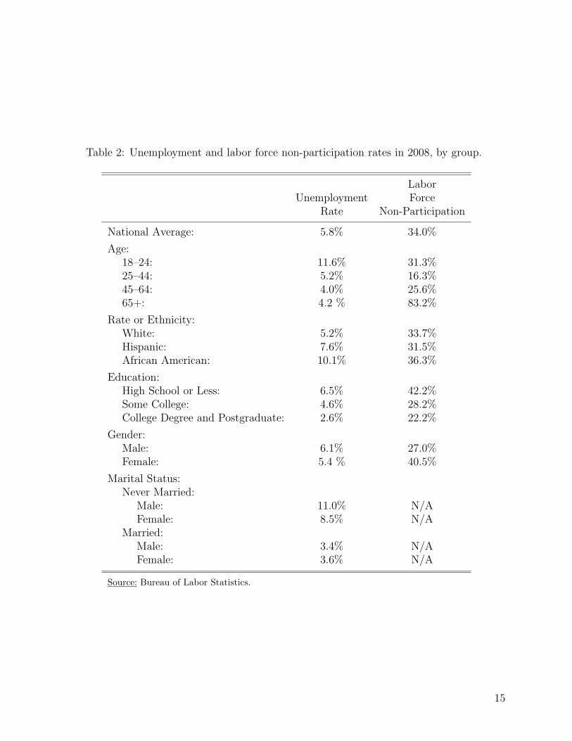
Table 2: Unemployment and labor force non-participation rates in 2008, by group.

LaborUnemployment Force

Rate Non-Participation

National Average: 5.8% 34.0%

Age:18–24: 11.6% 31.3%25–44: 5.2% 16.3%45–64: 4.0% 25.6%65+: 4.2 % 83.2%

Rate or Ethnicity:White: 5.2% 33.7%Hispanic: 7.6% 31.5%African American: 10.1% 36.3%

Education:High School or Less: 6.5% 42.2%Some College: 4.6% 28.2%College Degree and Postgraduate: 2.6% 22.2%

Gender:Male: 6.1% 27.0%Female: 5.4 % 40.5%

Marital Status:Never Married:

Male: 11.0% N/AFemale: 8.5% N/A

Married:Male: 3.4% N/AFemale: 3.6% N/A

Source: Bureau of Labor Statistics.

15

report unemployment rates inconsistent with theory.

A final clear pattern from Table 1 is that political independents report lower unemploy-

ment than Democratic party identifiers, and higher unemployment than Republican party

identifiers. There are multiple potential explanations for this result. One is that party

identification is associated with other variables that are related to higher local unemploy-

ment, and that we have imperfectly controlled for these variables in our analysis. Another is

that Democrats and Republicans perceive the economy differently (Gerber and Huber, 2009,

2010). In addition, previous research suggests that respondents may modify their responses

to economic questions to be more consistent with their vote choice or partisan identification

(Wilcox and Wlezien, 1993; Palmer and Duch, 2001).15 Because there was a Republican

president in 2008, Democrats may believe that unemployment is higher.16

While the results in Table 1 are consistent with respondents using information from their

community when forming perceptions of the unemployment rate, there are other covariates

in Table 1 that may provide more direct evidence that respondents are using information

from their surroundings. First, as shown in columns 3 and 4 of Table 1, a higher unemploy-

ment rate in a state is associated with a higher reported unemployment rate. Second, an

individual’s own unemployment status is associated with a higher reported unemployment

rate.

Finally, we can look at how unemployment perceptions vary across time. Figure 2 com-

pares the mean and median reported unemployment rates and the national unemployment

rate in October 2008 and October 2009. It shows that across these two points in time, higher

unemployment rates nationwide are correlated with higher average reported unemployment

15Gaines et al. (2007) finds less partisan difference when asking factual, rather than subjective, questionsabout the Iraq War casualties, suggesting the factual questions may be helpful for reducing this form ofsurvey bias.

16 This would be fairly straightforward to test by asking the same question when a Democratic presidentis in office. In 2009, respondents that identify as Democrats perceive unemployment to be insignificantlylower than Republicans, but estimates are hampered by a small sample size. Similar questions will be askedon the 2010 CCES.

16

Figure 2: Reported unemployment rates increase as the national unemployment rate in-creases.

0

2%

4%

6%

8%

10%

12%

14%

N = 2973 N = 1000

October 2008 October 2009

Mean Reported Unemployment

Median Reported Unemployment

National Unemployment

Notes: Reported unemployment is top-coded at 25% in order to reduce the influenceof outliers in the means. Means and medians are determined using sampling weights.

rates.17

5 Unemployment Perceptions and Vote Choice

We expect, based on the theory in Section 2, that the higher a respondent’s reported unem-

ployment level, the more likely he or she will be to vote for the candidate from the opposition

party, the Democrats. We regress an indicator variable coded one if the respondent indi-

cated he or she would vote for Barak Obama, the Democratic candidate, and zero if he or she

intended to vote for John McCain, the Republican candidate, on reported unemployment

17The correlates of reported unemployment rates are largely the same in 2009 as in 2008, with the exceptionof partisanship, as mentioned in Footnote 16. Another concern allayed by Figure 2 is that respondents aresimply picking a number in the middle of the range of historical unemployment given in the question.Ansolabehere, Meredith and Snowberg (2010) conducts comprehensive analyses of the effects of variouswordings of the question we focus on in this paper, and find that general patterns of response are the samewhether or not historical unemployment rates are included.

17

and a host of controls in Table 3.18 Mecro-economic voting predicts that the coefficient on

reported unemployment will be positive.

Table 3: Vote choice is correlated with unemployment perceptions.

Dependent Variable: Vote for Obama = 1, Vote for McCain = 0 (CCES)

Reported Unemployment 0.015∗∗∗ 0.003∗ 0.0002(0.002) (0.001) (0.001)

Reported Unemployment 0.068∗∗∗ 0.012∗∗ 0.009∗

(Report In Frame) (0.008) (0.005) (0.005)

Below Frame 0.29 0.014 0.003(0.18) (0.08) (0.07)

Above Frame 0.62∗∗∗ 0.11∗∗∗ 0.06(0.06) (0.04) (0.04)

Constant 0.42∗∗∗ 0.051∗∗∗ 0.10∗ 0.083 -0.005 0.049(0.02) 0.013 (0.059) (0.054) (0.31) 0.066

Party IdentificationNo Yes Yes No Yes Yes

(7 dummy variables)

All Other ControlsNo No Yes No No Yes

(From Table 1)

Observations 2574 2574 2492 2574 2574 2492

Notes: ∗∗∗, ∗∗, ∗ denote statistical significance at the 1%, 5% and 10% level with robust standarderrors in parenthesis. All specifications are implemented via OLS regressions.

The first column of Table 3 shows that reported unemployment is significantly correlated

with vote choice. However, as shown in Table 1, unemployment perceptions are correlated

with partisan leanings. In order to control for this, we enter dummy variables for each point

of a seven-point party identification scale in the second column. Reported unemployment is

still significantly related to vote choice, but the coefficient is smaller.

What other controls should be included in the regression? According to the theory above,

demographic factors are proxies for different economic experiences and local conditions, that,

18We use vote intention rather than reported choice because our unemployment perception question wasasked before the election. Using vote choice for the same respondents, which was reported after the election,produces somewhat stronger results. In particular, the coefficient on reported unemployment is significantat conventional levels, and positive, in all columns of Table 3.

18

in turn, cause individuals to have different perceptions. However, at the same time, demo-

graphic factors may have a direct effect on voting. Thus, although including demographic

controls will absorb much of the effect predicted by theory, they are necessary to avoid omit-

ted variable bias. The third column of Table 1 includes all our demographic controls in the

regression, and the coefficient on reported unemployment shrinks, as expected.

It is likely that respondents who reported an unemployment rate above or below the

historical unemployment rates, given in the survey question, were either not paying par-

ticular attention to the survey instrument, or have economic perceptions that significantly

diverge from the average respondent. Therefore, columns four through six group together

respondents who reported a level of unemployment above or below the range of historical

values—that is below 2.5% or above 10.8%, which we refer to in the table as the frame.19 For

those respondents who reported a level between 2.5% and 10.8%, reported unemployment

enters the specification linearly, as in the first three columns.

In our preferred specification, column five of Table 3, an increase in perceived unemploy-

ment from the rate for college graduates (2.6%) to 15% (the rate in various areas of the rust

belt in October 2008) results in a 20% increase in the probability that a respondent voted

for Obama.20 Thus, those respondents who believe that the unemployment rate is higher

19The reported unemployment rate of those above and below the frame is coded as zero in Table 3.We could also drop these respondents from the analysis—this produces similar results. We maintain allrespondents, as, in October 2008, there were areas (and groups) for which the unemployment rate was wellabove the historical high of the national rate, and thus, even a respondent paying close attention to thesurvey may report a high unemployment rate. Indeed, those who reported an unemployment rate above theframe were significantly more likely to vote against the incumbent.

20A one standard-deviation change in unemployment perceptions in this specification is associated withbeing six percent more likely to vote for Obama, which is the same as the standard deviation of two-partyvote in the postwar period. Probit or logit specifications produce qualitatively similar results, but strongersupport for mecro-economic voting. That is, the coefficients on reported unemployment are statisticallysignificant at greater levels, and the marginal effects of a change in perceptions are larger. We present OLSestimates as they are qualitatively similar and easier to interpret.

Up until this point, we have assumed a linear relationship between reported unemployment rate andvote choice. However, there is no particular reason to believe that the relationship should be linear. Aquadratic specification gives a similar magnitude for the relationship between reported unemployment andvote choice, and is statistically significant at the 95% level when including additional controls such asideology. Regressing unemployment on dummy variables for each percent of reported unemployment (24dummy variables) and running a joint F-test produces a generally increasing likelihood of voting for Obamaas reported unemployment increases, and the coefficients are jointly significant at p = 0.0000.

19

also tended to vote against the incumbent, as predicted.

6 Evidence from Time-Series Data

Although the patterns found in cross-sectional data comport with those expected from mecro-

economic voting, we can take our analysis a step further and analyze time-series data. In

particular, we analyze how state unemployment rates correlate with economic perceptions

and political support, after controlling for national trends. We find that both retrospective

economic evaluations and presidential approval within a state are significantly correlated

with state unemployment rates.21

As we posses limited time-series data on unemployment perceptions, we focus instead on

the standard retrospective economic evaluation from the American National Election Survey

(ANES), which asks:

Now thinking about the economy in the country as a whole, would you say that

over the past year the nation’s economy has gotten much better, somewhat better,

stayed about the same, somewhat worse, or much worse?

This question was asked from 1980 to 2008, with the exception of 2006.22

Based on our findings in the previous section, we expect that respondents in states with

higher unemployment rates, or states where unemployment increased dramatically in the

past 12 months, will report relatively worse retrospective evaluations than respondents in

states with low levels of unemployment. Table 4 shows this is the case. The first column

shows that the most important correlate of differences in retrospective economic evaluations

across time is the previous year’s change in the national unemployment rate. However, state

21We focus on states for both theoretical and practical reasons. From a theoretical prospective, monthlystate unemployment rates are reported by the Bureau of Labor Statistics and widely disseminated by themedia. From a practical prospective, state is the only geographic variable consistently reported in all of thedata sources we use.

22The 2006 ANES experimented with a 3 point scale, rather than a 5 point scale, and hence, is not directlycomparable.

20

unemployment rates, and the one year change in those rates, are also related to differences

in retrospective economic evaluations. In the second column, we replace the national un-

employment measures with year fixed effects. The results in this column are qualitatively

similar, but with smaller standard errors.

Table 4: State unemployment is correlated with national retrospective economic evaluations,even when controlling for national trends.

Dependent Variable: Average Retrospective Economic Evaluation in State (ANES)(-1 = Much Better, -5 = Much Worse)

State Unemployment Rate -0.020∗∗∗ -0.015∗∗ -0.034∗∗∗

(0.006) (0.006) (0.012)

∆ State Unemployment Rate -0.033 -0.059∗∗∗ -0.050∗∗∗

(0.022) (0.008) (0.010)

National Unemployment Rate -0.046(0.087)

∆ National Unemployment Rate -0.272∗∗∗

(0.060)

Constant -3.04∗∗∗ -4.01∗∗∗ -3.83∗∗∗

(0.63) (0.05) (0.08)

Year Fixed Effects No Yes YesState Fixed Effects No No Yes

State X Year Observations 497 497 497

Notes: ∗∗∗, ∗∗, ∗ denote statistical significance at the 1%, 5% and 10% level withrobust standard errors clustered by year in column 1, state in columns 2 and 3. Allspecifications are implemented via OLS regressions.

One concern with the specifications in columns 1 and 2 is that some states may have

chronically higher unemployment, and respondents in that state may generally be pessimistic

about the economy for non-economic reasons. To address this concern, we include state fixed

effects in column three. Once again, both the level and change in the state unemployment

rate are significantly correlated with national retrospective economic evaluations. The coef-

ficients imply that independent variation in state unemployment rates has about 25% of the

effect of similar variations in the national unemployment rate. Moreover, these findings are

21

in contrast to Books and Prysby (1999), which finds the level of state unemployment, but

not the change in state unemployment, was significantly related to respondents’ assessments

of unemployment as a national problem in the 1992 ANES.

Having observed that high state unemployment is correlated with economic perceptions

in aggregate time-series data, we now examine the extent to which state unemployment

affects political support. Specifically, we relate levels of, and one-year changes in, state un-

employment rates to presidential approval. To do so, we capture every Gallup poll on the

Roper Center Web site between 1981–2008 that reported presidential approval and the state

of residence for each respondent. We used these polls, 745 in all, to construct monthly pres-

idential approval rates for each state. These approval rates are regressed on unemployment

rates in Table 5.23

Table 5 shows that a one percent increase in the national unemployment rate is associated

with roughly a three percentage point decrease in presidential approval.24 Controlling for

national trends, an additional one percentage point state-level increase in unemployment

is associated with roughly a 0.6 percentage point decrease in approval. Thus, similar to

the results in Table 4, the independent correlation between state-level unemployment and

approval is roughly 20% of the national-level correlation. This contrasts with previous studies

that have found no effect of state unemployment on presidential vote share (Strumpf and

Phillippe, 1999; Eisenberg and Ketcham, 2004). Prior studies are hampered by the small

sample size imposed by using vote shares over the relatively short period where disaggregated

unemployment data is available. Our data provide greater statistical power to tease out the

relative importance of national versus state economic conditions.

There are two additional points worth noting, based on Table 5. The first is that changes

23The ANES does not have vote choice in non-presidential election years, but we can construct an indi-cator of presidential approval from these data using party thermometer ratings. Unfortunately, due to theneed to cluster standard errors, this does not provide enough power to examine the relationship betweenunemployment rates and party support. In particular, the standard errors are quite large. Therefore weturn to presidential approval data from the Gallup polls.

24The dependent variable in this analysis is the average approval in state where approving equals 100,disapproving equals -100, and neither approving or disapproving equals zero. Under this coding scheme, acoefficient of six corresponds to a three percentage point change in approval.

22

Table 5: State unemployment rates are correlated with presidential support.

Dependent Variable: Presidential Approval (Gallup)(100 = 100% approval, -100 = 100% disapproval)

National Unemployment Rate -6.44∗∗∗

(1.27)

∆ National Unemployment Rate 0.79(1.71)

State Unemployment Rate -1.22 -1.16∗∗∗

(1.20) (0.41)

∆ State Unemployment Rate 0.08(1.81)

State Unemployment:Under Reagan -1.03

(0.75)

Under Bush (I) -1.50∗∗∗

(0.39)

Under Clinton -0.97(0.65)

Under Bush (II) -1.36∗∗

(0.65)

Month X Year Fixed Effects No No Yes YesState X President Fixed Effects Yes Yes Yes Yes

State X Month Observations 4,545 4,545 4,545 Varies

Notes: ∗∗∗, ∗∗, ∗ denote statistical significance at the 1%, 5% and 10% level with robust stan-dard errors clustered at the state level (51 clusters). All specifications are implemented via OLSregressions. Column 4 contains the results of 4 separate regressions, one for each Presidency.

in either the national or state-level unemployment rate are uncorrelated with presidential

approval. This provides little support for retrospective voting. To the extent that voters

are retrospective, this indicates that we are investigating either the wrong time period (one-

year changes), or the wrong economic indicator (unemployment). Second, the correlation

between state unemployment and presidential approval is relatively consistent across all four

presidencies we examine.

Table 5 brings this study full circle: patterns of cross-sectional variation have lead us to

23

examine and discover patterns in aggregate, time-series data. Thus, using objective measures

of national economic performance as a proxy for economic perceptions underestimates the

effect of economic conditions on voter behavior. Moreover, focusing only on the national level

misses heterogeneity that may be informative about the mechanisms underlying economic

voting.

7 Discussion: The Shifting Nature of Economic Voting

We have shown that individual perceptions of macro-economic conditions are correlated with

an individual’s mecro-economic conditions. Specifically, using data from the 2008 CCES

we have shown that individuals who are members of groups that are more likely to be

unemployed report higher unemployment rates. Moreover, these perceptions are correlated

with political support: individuals who perceive the unemployment rate to be higher are more

likely to vote for the challenger, even after controlling for a host of other characteristics.

We have verified these patterns in aggregate, time-series, data. Both the standard ret-

rospective economic evaluation from the ANES, and presidential support from Gallup, vary

with state unemployment rates after controlling for national trends over the period from

1980–2008. Thus, as voters are influenced by their mecro-economies, vote patterns are af-

fected by the structure of the economy. This has particularly important implications for

election forecasting.

The U.S. economy has changed in many ways since the inaugural studies of economic

voting in the early 1970s. In particular, industries such as steel and auto manufacturing have

shrunk in both relative and absolute size, and services have become a much larger part of

the economy. Thus, an election forecasting model based on the pattern of economic voting

in the 1970s might be out of date by the mid-2000s. In general, forecasting models may

incorrectly predict support for the incumbent party, and the size of the error will depend

on both the size of the relative groups, which may shift across time, and the unemployment

24

rate of those groups. This is consistent with the fact that vote share is sometimes several

standard deviations away from the predictions of economic voting models. For example, the

original Fair (1978) economic voting model, which is based on macro-economic variables,

was updated many times in order to produce more accurate estimates. Even so, in 2004, this

model produced results that were off by as much as four standard deviations (Fair, 2006).25

This brings us back to the Kramer (1983) critique of using individual level data to un-

derstand economic voting. Kramer maintained that variation in individual level responses

to survey questions were largely noise, and thus, were either uninformative about, or pro-

duced biased understandings of, the mechanisms underlying economic voting. Our findings

challenge this critique in two ways. First, we have shown that individuals’ reports of eco-

nomic perceptions seem to incorporate real information about their economic conditions.

Moreover, we have verified this finding using aggregate data. Second, economic perceptions

are associated with differences in political support in both individual and aggregate data.

This turns the Kramer critique on its head: ignoring individuals’ economic perceptions and,

instead, using only macro-economic data runs the risk of creating a biased understanding of

economic voting.

25Note that at least one standard deviation may be due to the Iraq War, see Karol and Miguel (2008).

25

References

Alvarez, R. Michael. 1997. Information and Elections. Ann Arbor, Michigan: University ofMichigan Press.

Alvarez, R. Michael and Charles H. Franklin. 1994. “Uncertainty and Political Perceptions.”The Journal of Politics 56(3):671–688.

Alvarez, R. Michael and John Brehm. 2002. Hard Choices, Easy Answers: Values, Informa-tion, and American Public Opinion. Princeton, New Jersey: Princeton University Press.

Anderson, Christopher J., Raymond M. Duch and Harvey D. Palmer. 2000. “Heterogeneityin Perceptions of National Economic Conditions.” American Journal of Political Science44(4):635–652.

Anderson, Christopher J., Silvia M. Mendes and Yuliya V. Tverdova. 2004. “EndogenousEconomic Voting: Evidence from the 1997 British Election.” Electoral Studies 23(4):683–708.

Ansolabehere, Stephen, Marc Meredith and Erik Snowberg. 2010. “Asking About Numbers:Why and How.” California Institute of Technology, mimeo.

Ansolabehere, Stephen, Marc Meredith and Erik Snowberg. 2011. Sociotropic Voting andthe Media. In The ANES Book of Ideas, ed. John H. Aldrich and Kathleen McGraw.Princeton University Press.

Bartels, Larry M. 1986. “Issue Voting under Uncertainty: An Empirical Test.” AmericanJournal of Political Science pp. 709–728.

Besley, Timothy and Stephen Coate. 1997. “An Economic Model of Representative Democ-racy.” Quarterly Journal of Economics 112(1):85–114.

Books, John and Charles Prysby. 1999. “Contextual Effects on Retrospective EconomicEvaluations the Impact of the State and Local Economy.” Political Behavior 21(1):1–16.

Downs, Anthony. 1957. An Economic Theory of Democracy. New York, NY: Harper Collins.

Duch, Raymond. and David Armstrong. 2010. “Comparing the Effect of Economic Atti-tudes and the Real Economy on Vote Choice.” Paper presented at the annual meeting ofthe Midwest Political Science Association 67th Annual National Conference, The PalmerHouse Hilton, Chicago, IL .

Duch, Raymond M. and Randolph T. Stevenson. 2008. The Economic Vote: How Politicaland Economic Institutions Condition Election Results. Cambridge University Press.

Egan, Patrick J. and Megan Mullin. 2010. “Turning Personal Experience into Political At-titudes: The Effect of Local Weather on Americans Perceptions about Global Warming.”Temple University, mimeo.

26

Eisenberg, Daniel and Jonathan Ketcham. 2004. “Economic voting in US presidential elec-tions: Who blames whom for what.” Topics in Economic Analysis and Policy 4(1):1–23.

Erikson, Robert S., Michael B. MacKuen and James A. Stimson. 2002. The Macro Polity.Cambridge, UK: Cambridge University Press.

Evans, Geoffrey and Robert Andersen. 2006. “The Political Conditioning of Economic Per-ceptions.” The Journal of Politics 68(1):194–207.

Fair, Ray C. 1978. “The Effect of Economic Events on Votes for President.” The Review ofEconomics and Statistics 60(2):159–173.

Fair, Ray C. 2006. “The Effect of Economic Events on Votes for President: 2006 Update.”Yale University, mimeo.

Gaines, Brian J., James H. Kuklinski, Paul J. Quirk, Buddy Peyton and Jay Verkuilen. 2007.“Same Facts, Different Interpretations: Partisan Motivation and Opinion on Iraq.” TheJournal of Politics 69(4):957–974.

Gerber, Alan S. and Gregory K. Huber. 2009. “Partisanship and Economic Behavior: DoPartisan Differences in Economic Forecasts Predict Real Economic Behavior?” AmericanPolitical Science Review 103(3):407–426.

Gerber, Alan S. and Gregory K. Huber. 2010. “Partisanship, Political Control, and EconomicAssessments.” American Journal of Political Science 54(1):153–73.

Hetherington, Marc J. 1996. “The Media’s Role in Forming Voters’ National EconomicEvaluations in 1992.” American Journal of Political Science 40(2):372–395.

Hibbs, Douglas A. 2006. Voting and the Macroeconomy. In The Oxford Handbook of Polit-ical Economy, ed. Barry R. Weingast and Donald A. Witman. Oxford University Presschapter 31, pp. 565–586.

Hiscox, Michael J. 2006. “Through a Glass and Darkly: Attitudes Toward InternationalTrade and the Curious Effects of Issue Framing.” International Organization 60(3):755–780.

Karol, David and Edward Miguel. 2008. “The Electoral Cost of War: Iraq Casualties andthe 2004 US Presidential Election.” The Journal of Politics 69(3):633–648.

Kiewiet, D. Roderick. 1983. Macroeconomics and Micropolitics. The University of ChicagoPress.

Kinder, Donald R. and D. Roderick Kiewiet. 1979. “Economic Discontent and PoliticalBehavior: The Role of Personal Grievances and Collective Economic Judgments in Con-gressional Voting.” American Journal of Political Science 23(3):495–527.

Kinder, Donald R. and D. Roderick Kiewiet. 1981. “Sociotropic Politics: The AmericanCase.” British Journal of Political Science 11(2):129–161.

27

Kinder, Donald R., Gordon S. Adams and Paul W. Gronke. 1989. “Economics and Poli-tics in the 1984 American Presidential Election.” American Journal of Political Science33(2):491–515.

Kramer, Gerald H. 1971. “Short-Term Fluctuations in US Voting Behavior, 1896-1964.” TheAmerican Political Science Review 65(1):131–143.

Kramer, Gerald H. 1983. “The Ecological Fallacy Revisited: Aggregate-versus Individual-level Findings on Economics and Elections, and Sociotropic Voting.” The American Po-litical Science Review 77(1):92–111.

Krause, George A. 1997. “Voters, Information Heterogeneity, and the Dynamics of AggregateEconomic Expectations.” American Journal of Political Science 41(4):1170–1200.

Lewis-Beck, Michael S. 1988. Economics and Elections: The Major Western Democracies.The University of Michigan Press.

Lewis-Beck, Michael S. and Martin Paldam. 2000. “Economic Voting: An Introduction.”Electoral Studies 19(2-3):113–121.

Luskin, Robert C. 1987. “Measuring Political Sophistication.” American Journal of PoliticalScience 31(4):856–899.

MacKuen, Michael B., Robert S. Erikson and James A. Stimson. 1992. “Peasants or bankers?The American electorate and the US economy.” The American Political Science Review86(3):597–611.

Osborne, Martin J. and Al Slivinski. 1996. “A Model of Political Competition with Citizen-Candidates.” The Quarterly Journal of Economics 111(1):65–96.

Palmer, Harvey D. and Raymond M. Duch. 2001. “Do Surveys Provide Representative orWhimsical Assessments of the Economy?” Political Analysis 9(1):58–77.

Popkin, Samuel L. 1991. The Reasoning Voter: Communication and Persuasion in Presi-dential Campaigns. Chicago: University of Chicago Press.

Strumpf, Koleman S. and John R. Phillippe. 1999. “Estimating Presidential Elections: TheImportance of State Fixed Effects and the Role of National Versus Local Information.”Economics and Politics 11(1):33–50.

van der Brug, Wouter, Cees van der Eijk and Mark Franklin. 2007. The Economy and theVote: Economic Conditions and Elections in Fifteen Countries. Cambridge UniversityPress.

Wilcox, Nathaniel and Christopher Wlezien. 1993. “The Contamination of Responses to Sur-vey Items: Economic Perceptions and Political Judgments.” Political Analysis 5(1):181–213.

Wlezien, Christopher, Mark Franklin and Daniel Twiggs. 1997. “Economic Perceptions andVote Choice: Disentangling the Endogeneity.” Political Behavior 19(1):7–17.

28

Zaller, John. 1992. The Nature and Origins of Mass Opinion. Cambridge, UK: CambridgeUniversity Press.

Zaller, John and Stanley Feldman. 1992. “A Simple Theory of the Survey Response: An-swering Questions versus Revealing Preferences.” American Journal of Political Science36(3):579–616.

29

Appendix

A.1 Formalization of Section 3

Here we consider a two period model where a continuum of individuals seek information in

order to make optimal savings decisions. Each individual uses information revealed in this

process about the effects of an incumbent politician’s economic policies to inform his sincere

vote. In the second period, each individual consumes his wages and savings: no choices are

made. The fact that there is a continuum of individuals, and employment and unemployment

are determined only by the policies of the incumbent politician in each period, means that

we can focus on the decision problems of a single individual, taking the decision of all other

individuals as given.

Consider an individual with a per period utility of consumption given by u(·), which is

continuous, strictly increasing, and strictly concave. At the beginning of the first period,

the individual is endowed with some amount ε, and may be employed at a wage w. The

individual saves an amount s from the first to the second period. His total expected utility

if he is employed in the first period, as a function of the unemployment rate in the second

period R ∈ (0, 1) is given by

U(s|R) = u(ε+ w − s) +Ru(s) + (1−R)u(w + s)

Fact 1 The optimal savings rate s∗ is in the interval(0, ε+w

2

)if the individual is employed

in the first period, and(0, ε

2

)if unemployed. s∗ is increasing in R.

We follow the citizen-candidate tradition in assuming that each politician’s policies are

known and fixed. However, we add a slight twist in that the effects of these policies on each

individual is unknown. Specifically, the individual’s personal unemployment rate R ∈ {L,H}

is either low L, or high, H, with L < H and L + H < 1. Although the individual votes

30

sincerely in the election, he knows he is not pivotal, and takes the probability that the

incumbent will be reelected as some exogenous probability ξ.

The individual believes each politician’s economic policies have a prior probability π of

generating a high unemployment rate for him. He also witnesses two imperfect signals of

his personal unemployment rate under the incumbent politician, his personal employment

situation, σE ∈ {0, 1}—equal to zero if he is unemployed, and one if employed—and the

unemployment rate σRi ∈ {0, 1} in his mecro-economy, where one indicates a high unem-

ployment rate, and zero a low unemployment rate. Signals are correlated with personal

unemployment rates in the following way: P (σRi =0|R=L) = ρ = P (σRi =1|R=H), where

ρ > 12.26 The probability an individual is employed if his personal unemployment rate is

high, P (σE =1|R= H), is 1−H, and so on.

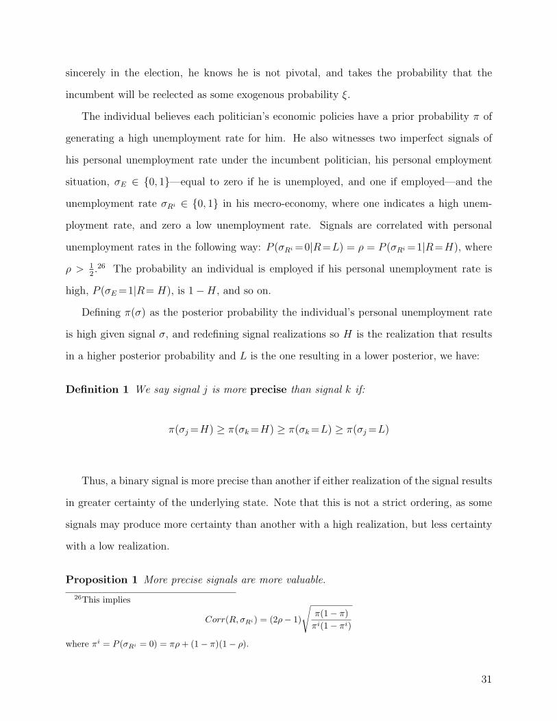
Defining π(σ) as the posterior probability the individual’s personal unemployment rate

is high given signal σ, and redefining signal realizations so H is the realization that results

in a higher posterior probability and L is the one resulting in a lower posterior, we have:

Definition 1 We say signal j is more precise than signal k if:

π(σj =H) ≥ π(σk=H) ≥ π(σk=L) ≥ π(σj =L)

Thus, a binary signal is more precise than another if either realization of the signal results

in greater certainty of the underlying state. Note that this is not a strict ordering, as some

signals may produce more certainty than another with a high realization, but less certainty

with a low realization.

Proposition 1 More precise signals are more valuable.

26This implies

Corr(R, σRi) = (2ρ− 1)

√π(1− π)πi(1− πi)

where πi = P (σRi = 0) = πρ+ (1− π)(1− ρ).

31

Returning to the particulars of our model, we make a simple assumption on the param-

eters of the signaling structure:

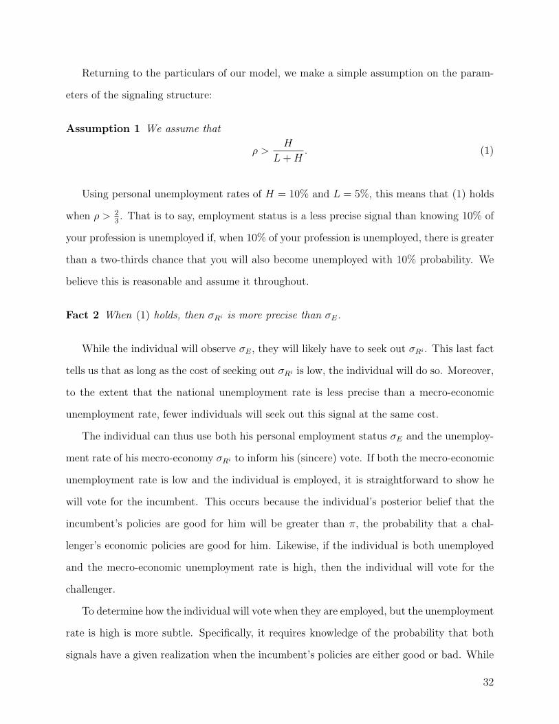
Assumption 1 We assume that

ρ >H

L+H. (1)

Using personal unemployment rates of H = 10% and L = 5%, this means that (1) holds

when ρ > 23. That is to say, employment status is a less precise signal than knowing 10% of

your profession is unemployed if, when 10% of your profession is unemployed, there is greater

than a two-thirds chance that you will also become unemployed with 10% probability. We

believe this is reasonable and assume it throughout.

Fact 2 When (1) holds, then σRi is more precise than σE.

While the individual will observe σE, they will likely have to seek out σRi . This last fact

tells us that as long as the cost of seeking out σRi is low, the individual will do so. Moreover,

to the extent that the national unemployment rate is less precise than a mecro-economic

unemployment rate, fewer individuals will seek out this signal at the same cost.

The individual can thus use both his personal employment status σE and the unemploy-

ment rate of his mecro-economy σRi to inform his (sincere) vote. If both the mecro-economic

unemployment rate is low and the individual is employed, it is straightforward to show he

will vote for the incumbent. This occurs because the individual’s posterior belief that the

incumbent’s policies are good for him will be greater than π, the probability that a chal-

lenger’s economic policies are good for him. Likewise, if the individual is both unemployed

and the mecro-economic unemployment rate is high, then the individual will vote for the

challenger.

To determine how the individual will vote when they are employed, but the unemployment

rate is high is more subtle. Specifically, it requires knowledge of the probability that both

signals have a given realization when the incumbent’s policies are either good or bad. While

32

there are a variety of ways to structure these probabilities, we assume that the signals are

conditionally independent, which can hold if the individual is a very small part of his mecro-

economy. That is, P (σE =e ∩ σRi =r|R) = P (σE =e|R) ∗ P (σRi =r|R).

Proposition 2 If ρ > 1−L2−L−H , then an individual’s vote choice will be determined by his

mecro-economic unemployment rate when he is employed, but his employment status when

he is unemployed. If ρ > HL+H

, as in (1), then an individual’s vote choice will always be

determined by his mecro-economic unemployment rate.

The proposition holds because being employed is an extremely weak signal that the

incumbent’s economic policies are good for the individual, and so it is easily outweighed by

the better signal of the unemployment rate in the individual’s mecro-economy.

As we argue in the text, some individuals will choose to become informed about the

national unemployment rate in addition to their mecro-economic unemployment rate. This

could be formalized here by assuming that each person has a cost of acquiring information

that is an i.i.d. draw from some distribution. As argued in the text, an individual’s mecro-

economic unemployment rate is a more precise signal than the national unemployment rate,

so this would mean that there is some subset of people who would pay the cost to acquire

information about the national unemployment rate, but this group of people would be smaller

than those who acquire information about their mecro-economic unemployment rate. Thus,

we do not formalize this here as the implications are straight-forward, and it would require

substantially more notation.

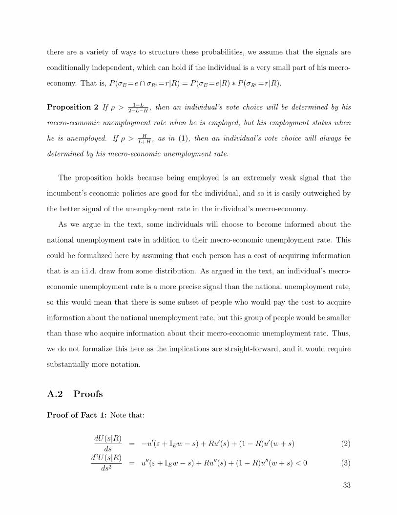
A.2 Proofs

Proof of Fact 1: Note that:

dU(s|R)

ds= −u′(ε+ IEw − s) +Ru′(s) + (1−R)u′(w + s) (2)

d2U(s|R)

ds2= u′′(ε+ IEw − s) +Ru′′(s) + (1−R)u′′(w + s) < 0 (3)

33

where IE is an indicator equal to one if the individual is employed in the first period. As (3)

indicates that U(s|R) is strictly concave, (2) will imply a unique equilibrium level of savings,

s∗. Setting s = 0 and s = ε+ IEw, respectively gives

dU(s|R)

ds

∣∣∣∣s=0

= −R(u′(ε+ IEw)− u′(0)) = −R∫ ε+IEw

0

u′′(x)dx > 0

dU(s|R)

ds

∣∣∣∣s=ε+IEw

= −u′(0) +Ru′(ε+ IEw) + (1−R)u′(ε+ IEw + w)

< −u′(0) + u′(ε+ IEw) =

∫ ε+IEw

0

u′′(x) < 0

so s∗ will be in the interior of (0, w). The integral representation follows from the fundamental

theorem of calculus. As (2) defines s∗, we can use implicit function theorem to (via implicit

differentiation) to determine

ds∗

dR= −

∂∂R

(dU(s|R)ds

)∂∂s∗

(dU(s|R)ds

) =

∫ w+s

su′′(x)dx

u′′(w − s) +Ru′′(s) + (1−R)u′′(w + s)> 0 (4)

Thus, s∗ is increasing in R, it is maximized when R = 1. When R = 1, s∗ solves

u′(ε+ IEw − s) = u′(s), that is, s∗ = ε+IEw2

. Thus, s∗ ∈(0, ε+IEw

2

). �

Proof of Proposition 1: Because of the independence property of preferences underlying

the utility representation, we can ignore the exogenous probability 1− ξ that the incumbent

will not be re-elected, as this will proportionally lower the value of all signals. Moreover,

without loss of generality, we can consider the case where ε = 0, and the individual is

employed in the first period. Recall that the individual has a prior belief π that his personal

unemployment rate will be high. Recall further that we defined the signal that results in

a higher posterior probability of the individual’s personal unemployment rate being high as

σ = L, the signal that results in a lower posterior probability of the individual’s personal

unemployment rate being high as σ = H. Here we denote P = Prob(σ = L).

34

Voters use Bayesian updating to determine the expected unemployment rate after getting

a signal. Recalling π(j) ≡ Prob(R=H|σ=j), and using the martingale property of Bayesian

updating, we have that

π = Pπ(L) + (1− P )π(H)

which, defining the expected unemployment rate R(j) ≡ (1− π(j))L+ π(j)H, as a function

of belief π(j), implies

R(π) = PR(L) + (1− P )R(H) (5)

as there is a one-to-one mapping between posterior probabilities and posterior expected

personal unemployment rates, we can think of a signal as having three characteristics, P ,

R(L), and R(H), where, according to (5) any two of these characteristics define the third.

By definition π(L) < π < π(H), which implies R(L) < R(π) < R(H). Define s∗j as the

optimal level of savings when the individual receives a realized signal σ = j. Using (4) we

have s∗L < s∗ < s∗H .

An individual values a signal because it allows him to better optimize his savings rate s∗.

The value of a particular realization of the signal can be defined as V (σ=j) = U(s∗j |R(j))−

U(s∗|R(j)). Thus, the total expected value of a signal is

V (σ) = PV (σ = L) + (1− P )V (σ = H). (6)

and we will examine how this value changes with the precision of the signal.

Reframing Definition 1: σ1 is more precise than σ2 if |L− R(σ1 =L)| ≤ |L− R(σ2 =L)|

and |H − R(σ1 =H)| ≤ |H − R(σ2 =H)|, with at least one strict inequality. To determine

if a more precise signal is indeed more valuable, we will examine how the value of the signal

changes with changes in the characteristics of a signal. However, as noted above, changing

one characteristic of the signal (P , R(L), and R(H)) necessitates a change in at least one of

the other characteristics so that (5) will continue to hold. Thus, we examine the three changes

in pairs of these variables holding the third constant. As any change can be represented by

35

some combination of these three changes, this is the same as investigating the basis of any

change.27

The first change is to increase the value of R(H), while fixing P . This will require a

compensating decrease in R(L) to maintain the equality in (5). That is

dV (σ)

dR(H)= P

dV (σ=L)

dR(H)+ (1− P )

dV (σ=H)

dR(H)

= P

[dU(s∗L|R(L))

dR(L)− dU(s∗|R(L))

dR(L)

]dR(L)

dR(H)+ (1− P )

[dU(s∗H |R(H))

dR(H)− dU(s∗|R(H))

dR(H)

]= P

[∫ s∗

s∗L

∫ w

0

u′′(y + x)dy dx

]dR(L)

dR(H)+ (1− P )

[−∫ s∗H

s∗

∫ w

0

u′′(y + x)dy dx

]

where the second line follows from the chain rule, and∫ s∗s∗L

∫ w0u′′(y + x)dy dx < 0 due to the

concavity of u. Note that within each square bracket the first derivative is made simpler

by the envelope theorem, and the second is zero as s∗ is fixed. Re-arranging (5) yields

R(L) = R(π)−(1−P )R(H)P

, so

dR(L)

dR(H)=P − 1

P< 0, (7)

and thus, dV (σ)dR(H)

> 0. Note that (7) is negative, as expected.

A second change is to increase P while fixing R(L). This implies an increase in R(H),

dR(H)dP

= R(H)−R(L)1−P > 0. Now

dV (σ)

dP= U(s∗L|R(L))− U(s∗|R(L))−

[U(s∗H |R(H))− U(s∗|R(H))

]+ (1− P )

dV (σ=H)

dR(H)∗ dR(H)

dP

= u(w − s∗L) +R(L)u(s∗L) + (1−R(L))u(w + s∗L)−(u(w − s∗H) +R(L)u(s∗H) + (1−R(L))u(w + s∗H)

)= U(s∗L|R(L))− U(s∗H |R(L)) > 0

where the second line follows from expanding V (·) and U(·) into component u(·) terms, and

canceling, the third line follows from the definition of U(·), and the inequality follows from

27Mathematically, this is a derivative on a three dimensional surface, and the pairwise changes establishchanges along a set of basis vectors. Changes in all three variables simultaneously are combinations ofchanges along these basis vectors. For simplicity, we avoid vector calculus notation.

36

the definition of s∗L.

A final change is to increase R(L) while fixing R(H). This implies an increase in P ,

dPdR(L)

= PR(H)−R(L)

> 0. The effect of this final change is:

dV (σ)

dR(L)= P

dV (σ=L)

dR(L)+(V (σ=L)− V (σ=H)

) dP

dR(L)

=P

R(H)−R(L)

[dV (σ= l)

dR(L)

(R(H)−R(L)

)+ V (σ=L)− V (σ=H)

]=

P

R(H)−R(L)

[u(w − s∗L) +R(H)u(s∗L) + (1−R(H))u(w + s∗L)−

[u(w − s∗H) +R(H)u(s∗H) + (1−R(H))u(w + s∗H)

]]=

P

R(H)−R(L)

[U(s∗L|R(H))− U(s∗H |R(H))

]< 0

where, once again, the third line follows from expanding V (·) and U(·) into component u(·)

terms, and canceling, the fourth line follows from the definition of U(·), and the inequality

follows from the definition of s∗H .

Note that in all three of these changes, an decrease in |H − R(H)| or |L − R(L)| is

associated with an increase in the value of the signal. Thus, more precise signals are more

valuable. �

Proof of Fact 2: Start by re-writing (1) as the first inequality below:

ρ

1− ρ>H

L>

1− L1−H

. (8)

The second inequality follows from the fact that H > L and L+H < 1. We have that

ρ(1− π)L > H(1− π)(1− ρ)

πρ(πH + (1− π)L) > πH(πρ+ (1− π)(1− ρ))

π(σRi =1) =πρ

πρ+ (1− π)(1− ρ)>

πH

πH + (1− π)L= π(σE =1).

37

Using the second inequality in (1) we have

ρ(1− π)(1−H) > (1− ρ)(1− π)(1− L)

π(1−H)(π(1− ρ) + (1− π)ρ) > π(1− ρ)(π(1−H) + (1− π)(1− L))

π(σE =0) =π(1−H)

π(1−H) + (1− π)(1− L)>

π(1− ρ)

π(1− ρ) + (1− π)ρ= π(σRi =0).

Thus, π(σRi =1) > π(σE =1) > π(σE =0) > π(σRi =0), so σRi is more precise than σE. �

Proof of Proposition 2: If the individual is employed, but the unemployment rate is high

in the individual’s mecro-economy, then he will vote for the challenger when

π(1− ρ)(1− L)

(1− π)ρ(1−H) + π(1− ρ)(1− L)< π ⇐⇒ ρ >

1− L2− L−H

. (9)

which is assumed to be true as in (8). If, instead, the individual is unemployed, but the

unemployment rate is low, then the individual will vote for the incumbent when

πρL

πρL+ (1− π)(1− ρ)H> π ⇐⇒ ρ >

H

L+H, (10)

which is satisfied whenever (1) is true. �

38