medical insurance and the use of health care services by ... · medical insurance and the use of...

E L S E V I E R Journal of Health Economics 16 (1997) 129- ! 54

JOURNAl. OF IEEP.LTH

ECONOMICS

Medical insurance and the use of health care services by the elderly

Michael D. Hurd a,b, Kathleen McGarry c,b,, a Department of Economics, SUNY Stony Brook, New York, NY, USA

b NBER, Cambridge, MA 01238, USA Department of Economics, Unir'ersity of California, Los Angeles, CA 90095-1477, USA

Received 1 March 1995; accepted | June 1996

Abstract

The objective of this paper is to find how health insurance influences the use of health care services by the elderly. On the basis of the first wave of the Asset and Health Dynamics Survey, we find that those who are the most heavily insured use the most health care services. Because our data show little relationship between observable health measures and either the propensity to hold or to purchase private insurance, we interpret this as an effect of the incentives embodied in the insurance, rather than as the result of adverse selection in the purchase of insurance. © 1997 Elsevier Science B.V. All rights reserved.

JEL classification: I12; J14

Keywords: Medicare; Health insurance; Medical services

I. Introduction

The e lder ly are heav i ly insured against hea l th care costs: o v e r 9 5 % o f all

e lder ly (65 or ove r ) are c o v e r e d by Med ica re , w h i c h p rov ides heal th insurance at

g rea t ly subs id ized rates. In addi t ion, m a n y have pr iva te supp lemen ta l c o v e r a g e

wh ich r e duc e s or e l imina tes the M e d i c a r e deduc t ib les and c o - p a y m e n t s . The re fo re ,

they face little m o n e y cos t fo r a w ide range o f m ed i ca l services . T h e goal o f this

Corresponding author. Department of Economics, UCLA, Los Angeles, CA 90095-1477. Fax: (310) 825-9528; e-mail: [email protected].

0167-6296/97/$17.00 © 1997 Elsevier Science B.V. All rights reserved. PII S0 1 6 7 - 6 2 9 6 ( 9 6 ) 0 0 5 1 5-2

130 M.D. Hurd, K. McGarry / Journal of Health Economics 16 (1997) 129-154

paper is to provide quantitative evidence about how this affects the consumption of medical services by the elderly.

We use data from the Asset and Health Dynamics Survey (AHEAD), a new nationally representative survey of the population 70 or over, to estimate the effect of insurance holdings on the use of doctor and hospital services by elderly individuals. Because any observed relationship between insurance coverage and service use could be the result of adverse selection, we first study the determinants of having and of purchasing private health insurance. We pay particular attention to the relationship between a variety of indicators of health status and the likelihood of holding private insurance. As determined in this way, we find little evidence for adverse selection by observed health status in the holding of private insurance. ~ Rather, having insurance seems to be based primarily on economic resources: those with greater income and wealth are more likely to have supplemental coverage. In agreement with other studies we find that insurance holdings affect service use: those with the most coverage have the highest probabilities of visiting a doctor or staying in a hospital.

2. Previous studies

The relationships between insurance and service use, and between service use and health outcomes among the non-elderly, is well documented in studies based on the RAND Health Insurance Experiment (Newhouse et al., 1993). The RAND experiment randomly assigned individuals to health insurance plans that varied in co-payments and deductibles. According to the experimental results, greater liability by the patient for health care services decreased health expenditures significantly. Individuals with the largest cost-sharing had expenditures up to 30% less than those with no cost-sharing provisions.

The RAND study provides valuable evidence of the effect of health insurance on demand for services because it was designed as a true experiment. In non-experimental situations an analysis of the effect of insurance coverage is complicated by adverse selection, i.e. the purchasing of insurance in anticipation of above-average consumption (Rothschild and Stiglitz, 1976; Wilson, 1977). Apparently adverse selection is sufficiently widespread that it can be detected empirically, and several papers have provided evidence of selection in the non-elderly population (Price and Mays, 1985; Marquis and Phelps, 1987). 2

It is not clear, however, whether these results, based on studies of the non-elderly, can be generalized to the elderly population. One would expect the

I Although we will often use the term 'adverse selection' , we mean adverse selection by observed

health status. We cannot rule out the possibility of adverse selection with respect to unobservable

characteristics such as tastes for medical care that would cause someone who intends to use health care

services intensively to purchase insurance in anticipation.

2 See also Newhouse (1996) for a summary.

M.D. Hurd, K. McGarry / Journal of Heatth Economics 16 (1997) 129-154 131

behavior of the elderly to differ from that of the non-elderly for several reasons. First, a substantial fraction of the medical expenditures of the elderly are already covered by Medicare, part of which is available free of charge, and part of which is heavily subsidized. Thus adverse selection should occur only in the market for insurance to supplement Medicare. Secondly, additional coverage is provided for the poor elderly through Medicaid. Because Medicaid and Medicare together provide almost complete coverage, those enrolled in Medicaid have little reason to purchase further insurance. Furthermore, under current law some of those who do not qualify for Medicaid on the basis of their financial situation, would qualify for Medicaid if their medical expenditures were to become large. These two factors ought to reduce the extent of adverse selection among the elderly.

Previous work examining the decision by the elderly to purchase private insurance has provided conflicting evidence of adverse selection. Wolfe and Goddeeris (1991) found that those with large past expenditures were significantly more likely to hold private supplemental insurance; yet, those whose health was poor were no more likely to hold private insurance than those in good health. Eggers and Prihoda (1982) found that when Medicare recipients were given a choice of enrolling in an HMO or continuing with a fee-for-service program, the healthier elderly chose the HMO while the less healthy remained with a fee-for- service plan, providing some evidence of adverse selection. 3 More recent work by Ettner (1995) and Lillard and Rogowski (1995) found little difference by health status in the probability of purchasing private insurance. Therefore, any selection would have to be by unobserved tastes for service use, but those tastes are not related to health status.

The empirical evidence about the effects of insurance on service use by the elderly (often termed 'moral hazard') is more consistent: additional insurance coverage is associated with increased service use (Link et al., 1980, McCall et al., 1991, Lillard and Rogowski, 1995). 4

We conclude that while the empirical literature does demonstrate a strong correlation between insurance coverage and service use, the literature does not provide consistent evidence of the role for adverse selection in having insurance. In this paper we aim to quantify both the importance of adverse selection in the market for private insurance among the elderly, and the role of insurance coverage in influencing consumption. Although we cannot eliminate the possibility that unobserved tastes play a role, because of the quality of our data, we can account for a wider range of health indicators and economic variables than in previous studies while controlling for differences in income and wealth.

3 See Hellinger (1995) for a discussion of selection into HMOs. 4 Of course, some of the affects attributed to insurance could be a result of unobserved adverse

selection.

132

3. Data

M.D. Hurd, K. McGarry / Journal of Health Economics 16 (1997) 129-154

The Asset and Health Dynamics Survey (AHEAD) is a new panel survey of individuals born in 1923 or earlier and their spouses or partners. When appropri- ately weighted, the sample is representative of the non-institutional population from these cohorts. Our study is based on the first round of interviews which was conducted in late 1993 and early 1994.

AHEAD is well suited for a study of health care demand among the elderly population. It has information about six types of service use. Respondents were asked if, in the past year, they had been to a doctor, and if so the number of times; whether they had been to the hospital or (separately) to a nursing home, and if so the number of nights they stayed; whether they had had outpatient surgery; whether they had had home health care; and whether they had seen a dentist. For each type of service use the respondent was asked if there were any expenses that were not covered by insurance. Respondents were asked to estimate total out-of- pocket expenditures over a year for all services.

AHEAD measured health status along a number of dimensions. Health is self-rated as excellent, very good, good, fair, or poor. AHEAD also has an extensive battery of questions about disease and health conditions. For example it asked: "Has a doctor ever told you that you had..." a heart attack, a stroke, cancer? It also asked about chronic conditions such as high blood pressure, diabetes and incontinence. Up to six limitations to activities of daily living (ADLs) (dressing, bathing, toileting, eating, getting in and out of bed, and walking across a room) and five limitations to instrumental activities of daily living (IADLs) (using a telephone, shopping, cooking, taking medication, and managing money) were assessed.

We used innovative questions in AHEAD in which the individual reports a subjective probability of survival, and the probability of entering a nursing home within five years. Both measures ought to be related to the individual's perception of future health status, and they have a numerical scaling that is missing from the commonly used self-assessed health status. Thus, they may be useful in uncover- ing adverse selection in that they reveal private information about future health status and, by extension, health expenditures.

AHEAD asked respondents if they were covered by Medicare, and if so, coverage under Part B. They were also asked: " Is your health care currently covered by Medicaid?" and about veterans' insurance. 5 With respect to private insurance, respondents were asked if they had any other health insurance, the type

5 We classify someone as having veterans' benefits if they answer yes to the question: "Are you currently covered by any government health insurance programs such as Railroad Retirement, CHAMPUS, CHAMPVA, or other military programs?"

M,D. Hurd, K. McGarry / Journal of Health Economics 16 (1997) 129-154 133

of insurance (including the coverage of long-term care), and total premiums paid. 6 Unfortunately, AHEAD did not ascertain whether the policy was related to (or subsidized by) past employment, or about the services covered by the policy, such as prescription drugs. 7

AHEAD measured both income and assets. This is important because economics status and health are strongly correlated in the AHEAD data. For example, we calculated that mean non-housing wealth of a 70-74 year old in excellent health was $220,500 but just $37,900 for someone in poor health. 8 An implication is that studying the relationship between insurance purchase and health without adequately controlling for economic status could well obscure adverse selection: if the well-to-do elderly purchase health insurance to protect their sizable assets, and the unhealthy elderly also purchase health insurance to cover their greater-than- average health expenditures, there could be little apparent correlation in the data between health status and insurance purchase, even though adverse selection is important.

Our focus in this paper is on the holdings and purchase of private insurance, and the effect of these holdings on the use of health services. We will ignore two other margins of choice relating to insurance. The first is spend-down to Medicaid eligibility, the study of which is best done with panel data. The second is the purchase of Part B of Medicare: about 5% of those with Part A do not purchase Part B. As we shall see later, however, this does not appear to be caused by health status but by individual attitudes toward insurance, or perhaps constraints imposed by personal finances. 9

The complete AHEAD sample consists of 8224 observations, but it is population-representative only of those aged 70 or over at baseline. ~0 To make population comparisons we deleted those who were less than 70 years old (783). We also eliminated those who did not finish the survey, and, therefore, have no valid observations for many variables (114). The resulting sample has 7327 observa-

6 Our data do not distinguish insurance associated with an HMO from other types of policies. 7 Under the Omnibus Budget Reconciliation Act of 1990 (OBRA 1990) private insurance policies

that supplement Medicare (medigap policies) are restricted to be one of 10 types. 'Other insurance' in our sample will frequently refer to a policy that differs from these 10 types for two important reasons. First, medigap insurance is purchased when an individual first purchases Part B of Medicare, which is most likely at age 65. Our sample consists of those 70 and over in 1993 and therefore many would have purchased medigap insurance prior to the restrictions on policies that took effect in 1992. These individuals are permitted (in most states) to retain their coverage even if it is other than one of the 10 types. Secondly, 'other insurance' in our sample may not be true medigap but may come from a prior (or current) employer. These plans will also differ from the 10 standard medigap policies.

8 See Smith (1995) for many similar findings relating to health status and wealth. 9 Estimates from AHEAD of Medicare coverage, Medicaid coverage, and private insurance coverage

are close to coverage rates reported by Social Security and estimated from the National Medical Expenditure Survey. See an earlier draft of this paper (1994) for these comparisons.

10 We use the 'post-alpha' release of AHEAD.

134 M.D. Hurd, K. McGarry / Journal o f Health Economics 16 (1997) 129-154

tions. Sample sizes in some of the regressions and cross-tabulations vary due to missing values. When warranted, we include dummy variables for missing values and assign a value of zero to the missing variable.

4. Insurance holdings

Medicare pays for approximately 45% of the medical expenses of the elderly (National Academy on Aging, 1995). To pay lbr services not covered by Medi- care, and the deductibles and co-payments associated with Medicare, some individuals buy insurance in the private sector. Others may receive coverage from a former employer as part of a retirement package. As shown in Table 1, most individuals (70%) have both Medicare and some other kind of private health insurance. Smaller but significant fractions have Medicare only (17%) or both

Table 1 Means and distribution of variables by insurance status

Type of insurance

None Medicaid Medicare Medicare Other only and other only

Family wealth (thousands): mean total wealth 59.1 26.8 128.7 203.5 311.2 median total wealth 28.5 0.6 42.7 111.2 141.1 mean non-housing 30.0 9.5 65.0 122.4 219.7 median non-housing 3.2 0.2 6.4 41.1 44.6 Family income (thousands): mean income 11.1 8.7 17.5 25.4 37.6 median income 8.0 7.2 12.0 20.0 22.5 Age: 77.7 79.3 78.7 77.4 76.3 Healtt, status: excellent 0.09 0.05 0.09 O. i 2 O. 11 very good O. 16 O. 10 0.21 0.25 0.39 good 0.33 0.25 0.28 0.32 0.25 fair 0.23 0.29 0.25 0.22 O. 19 poor O. 19 0.32 O. 16 0.09 0.07 Services: saw doctor (%) 66 92 84 91 90 number of visits (pos) 8.55 7.36 5.56 5.27 4.88 went to hospital (%) 27 36 2t 22 19 number of nights (pos) 13.67 13.19 12.00 10.25 14.96 Number of observations: 56 787 1196 4983 118 Percent o f total: 0.8 11.1 16.8 69.8 1.7

Note.- 187 individuals who do not know their insurance status are omitted.

M.D. Hurd, K. McGarry / Journal of Health Economics 16 (1997) 129-154 135

Medicare and Medicaid (10%). Less than 1% of this sample has no insurance, attesting to the inclusiveness of the Medicare and Medicaid programs.

Those who have Medicare and other (private) insurance consistently have higher wealth and higher income, and they are healthier than those without private insurance. Ninety-one percent saw a doctor during the year; yet conditional on having a visit, they have fewer visits than any group except for 'other only': for example, 5.3 visits compared with 7.4 for those with both Medicare and Medicaid. They had a rather low frequency of a hospital stay, and if they did have a stay the number of nights was the least, 10.2. These figures give additional evidence of their better health.

The Medicaid population is poor indeed. Their mean wealth is just under $27,000 and mean family income is $8700. Their health is worse than other groups as measured by self-assessment, and they had hospital stays with greater frequency.

Those with insurance coverage but not Medicare or Medicaid ( 'other only') have the highest income and wealth, and they seem to be the healthiest as measured by the fraction in good to excellent health. They also have the fewest visits to a doctor conditional on at least one visit, t2

5. Private insurance

Our data are somewhat deficient in that we do not know whether private insurance is purchased in the market or employer-provided: no direct distinction is made in the questionnaire. We do know how much, if anything, someone pays for health insurance, but this information cannot be used to establish conclusively whether the insurance is provided through a former employer because retiree health insurance often requires some portion of the premium to be paid by the retiree.

5.1. Insurance holdings

In cross-tabulations (not shown) that control for age, and income and wealth, the fraction that has private insurance is highest among those in better health, and the variation is substantial. For example, among 70-74 year olds in the second

~ Among the non-elderly almost 16% were uninsured in 1989 (U.S. Bureau of the Census, 1993). lz One might imagine that this 'other only' group consists largely of those who are still employed. (In

fact 12% are employed compared with just 10% of the Medicare and other group and 7% of the Medicare only group.) If an individual has health insurance on a current job, then Medicare is the secondary payer. However, since Part A is free to eligible individuals, there is no incentive not to enroll in the program despite having employer-provided coverage.

136 M.D. Hurd, If. McGarry / Journal o f Health Economics 16 (1997) 129-154

income and wealth quartile, 84% of those in very good health have private insurance compared with just 69% of those in fair health. This kind of variation is typical.

To control for the many additional factors which are likely to influence the holding of private insurance we estimate a probit model for the probability of having private insurance. Table 2 shows in the column labeled 'Effect ' the probit coefficients multiplied by the normal probability density evaluated at the population probability. Thus they have the interpretation of a change in probability for a change in the particular covariate. The column labeled 'Square root of chi-square' can be used to test the null hypothesis that an effect is zero: a 5% level test would reject if this statistic is greater than 1.96. Adverse selection along the lines of observed health status would predict that those in poor health would be more likely to hold insurance than those in excellent health. We control for holdings of public insurance, financial status and demographic characteristics in addition to detailed health measures. We include health or disease conditions that are perma- nent enough that there would be opportunity between onset and the AHEAD interview to purchase insurance in response to onset.

We estimate that someone with Medicare Part A but not Part B will have a frequency of private insurance 0.085 lower than someone with Part B, the reference group. One explanation is that those who choose not to purchase Part B want less total coverage, so they are less likely to have private insurance. However, the result is more likely due to a joint decision: the 10 medigap policies are specifically designed to supplement Medicare (Parts A and B), and, therefore, are only fully useful to those with Part B. 13 Furthermore, because Part B is heavily subsidized (individuals pay only 25% of the true cost) the first dollar spent on insurance will purchase more insurance if used to buy Part B than a supplemental policy. 14

The other combinations of insurance coverage have sensible effects: those with coverage from Medicaid or other government sources are already well covered and are much less likely to have other insurance. 15 The probability of having private insurance is about 0.43 lower for this group than for someone with Medicare Parts A and B.

Contrary to what we would expect with adverse selection, subjective health status has virtually no effect on insurance holdings. A change in health has little systematic effect on the likelihood of having private insurance, and, in fact, the

13 See Physician Payment Review Commission (1996). ~4 These statements are not necessarily true of employment-related private insurance, which may not

be designed to supplement Medicare, and which may be subsidized by an employer. Such employer- provided insurance likely explains why the reduction in the probability is not larger.

is Note that by law the Medicaid program purchases Medicare Part B for its enrollees already participating in Part A of Medicare.


Table 2

Probit analysis of the probabil i ty of having private insurance: Insurance, heal th and economic effects (Average probabi l i ty is 0,738)

Effect Square root of

chi-square

Insurance status: Medicare Parts A and B (omitted) - -

Medicare A only - 0 . 0 8 5 3.39

Neither Medicare nor Medicaid - 0 . 0 2 7 0.70

Medicare and Medicaid - 0 . 4 3 1 18.37

veterans - 0.428 14.53

Self-reported health: excellent 0.009 0.34

very good 0.020 0.95

good (omit ted) - -

fair 0.011 0.50

poor - 0.032 1.13

excellent or very good and bet ter - 0.084 2.56

excellent or very good and worse 0.016 0.34

good and bet ter - 0 . 0 3 5 1.05

good and worse 0.032 0.95

fair or poor and better - 0.037 1.13

fair or poor and worse - 0 . 0 4 2 1.82

Health conditions: has at least one condit ion 0.025 1.02

high blood pressure 0.015 1.03

diabetes 0.004 0.19

cancer 0.076 3.78

lung 0.006 0.22

lung problems limit activity - 0 . 0 3 7 0.96

heart condit ion 0.038 2.29

angina 0.026 0.99

stroke 0.008 0.26

problems remaining from stroke 0.057 1.47

psychiatr ic problems - 0 .010 0.47

fell in past year - 0 . 0 2 3 1.32

fell and was injured 0.046 1.67

incont inence 0.013 0.78

bothered by pain - 0.006 0.41

other health problems 0.064 4.26 Other health measures: prob. enter nursing home - 5 yr 0.032 0.99

prob. l ive 11 15 yr - 0.063 2.79 currently smokes - 0.045 2.00

former smoker 0.017 1.15 never smoked (omit ted) - -

low BMI - 0.013 0.71

h igh BMI - 0.001 0.04

138 M.D. Hurd, K. McGarry / Journal o f Health Economics 16 (1997) 129-154

Tab le 2 ( c o n t i n u e d )

Ef fec t Squa re root o f

c h i - s q u a r e

Income and wealth quartiles: wea l th t * i n c o m e 1 - 0 .237 7.81

wea l th 1 * i n c o m e 2 - 0 .187 5.85

wea l th 1 * i n c o m e 3 - 0 .155 3 .82

wea l th 1 * i n c o m e 4 0 .073 0 .62

w e a l t h 2 * i n c o m e 1 - 0.171 5 .36

w e a l t h 2 * i n c o m e 2 - 0 .082 2 .84

w e a l t h 2 * i n c o m e 3 0.011 0 .35

w e a l t h 2 * i n c o m e 4 - 0 .052 1. I 0

wea l th3 * i n c o r n e 1 - 0 .143 3 .48

wea l th3 * i n c o m e 2 - 0 .078 2 .48

wea l th3 * incorne3 0 .015 0 .46

wea l th3 * i n c o m e 4 0 .018 0.51

w e a l t h 4 * i n c o m e I - 0 .072 1.08

w e a t t h 4 * i n c o m e 2 0 .020 0.41

w e a l t h 4 * i n c o m e 3 - 0 .036 1.08

w e a l t h 4 * i n c o m e 4 (omi t t ed ) - -

O w n h o m e 0 .053 3 .44

P e n s i o n i n c o m e 0 .143 9 .57

Age: 7 0 - 7 4 yrs o ld (omi t t ed ) - -

7 5 - 7 9 yrs o ld 0 .004 0 .26

8 0 - 8 4 yrs o ld - 0 . 0 1 6 0 .86

8 5 - 8 9 yrs o ld 0 .008 0.35

90 and o lder 0 ,046 1.29

Cognitive score: l owes t quar t i l e - -

s e c o n d quar t i l e 0 .102 4 ,49

th i rd quar t i l e 0 .144 5.83

fou r th quar t i l e 0 .169 6 .45

Schooling level: f e w e r than 9 yrs - 0 .085 4 .62

9 - 1 1 yea r s - 0 .007 0 ,35

12 yea r s (omi t t ed ) - -

m o r e t han 12 yea r s - 0 .003 0 .15

Other demographic variables mar i t a l s t a tus (1 i f ma r r i ed ) 0 .017 0 .93

m a l e - 0 ,077 4.71

f inanc ia l r e s p o n d e n t - 0 .046 2 .30

n o n - w h i t e 0 .215 13.08

N u m b e r o f o b s e r v a t i o n s 7202

Note: Ef fec t s are par t ia l de r iv i t i ve s de r i ved f r o m probi t e s t ima te s . Squa re root o f c h i - s q u a r e is

a s y m p t o t i c a l l y the abso lu t e v a l u e o f a s t anda rd n o r m a l u n d e r the nul l h y p o t h e s i s tha t the e f fec t is zero.

M e a n o f the d e p e n d e n t va r i ab le is 0 .738. P s e u d o R 2 is 0 .36 . W e a l t h l r e fe r s to the l o w e s t wea l th

quar t i le and w e a l t h 4 re fe rs to the h ighes t . S i mi l a r l y for i n c o m e quar t i l es . Va r i ab l e s d e n o t i n g m i s s i n g

va lue s for i n s u r a n c e s ta tus , the p robab i l i ty o f en t e r ing a n u r s i n g h o m e , the su rv iva l p robabi l i ty , a n d

cogn i t i on score are i nc l uded in the e s t i m a t i o n bu t not repor ted .


only significant coefficient (on excellent or very good health which has improved over the past year) does not support adverse selection: under adverse selection, controlling for current health, those whose health had been worse previously, should have more insurance than those with the same current and past health, not less as we find here. This result is not in accordance with the results of Wolfe and Goddeeris (t991), who find adverse selection based on lagged health. Of the 16 health conditions, only cancer, heart conditions, and 'other health problems', are statistically significant, but the numerical magnitudes of the coefficients are small. Furthermore, as a group the conditions are not statistically significant at the 5% level, and in results not shown here, their inclusion has very little effect on the coefficients of the other variables such as insurance.

Mild evidence of adverse selection by health comes from the significant coefficient on the subjective probability of living 11-15 more years. This variable is likely to be correlated with unobserved health status, and here those who consider themselves likely to live considerably longer have a lower probability of having insurance. However, the numerical magnitude is small: a variation in the subjective probability of living of 0.5 is substantial, and even that is associated with a probability change of just 0.032.

Current smokers have a lower probability of holding private health insurance, reflecting perhaps their attitudes towards health or towards risk in general. Those who formerly smoked, however, are neither more nor less likely than non-smokers to hold private insurance. Again, this provides no evidence for adverse selection as smokers would be expected to face higher medical expenses than non-smokers. We also included in the specification two variables which indicate if the individual's body mass index (BMI) is either exceptionally low (lowest 15%) or exceptionally high (highest 15%). 16 These can be thought of as additional measures of health. Neither variable has significant explanatory power.

Just as we saw in Table 1 and as we discussed earlier, wealth and income are strongly associated with having private insurance. For example, someone in the lowest income and wealth quartiles is about 24 percentage points less likely to have private insurance than someone in the top quartiles. This difference is after controlling for the large negative effect of having Medicaid, which many in these lower quartiles would have. Furthermore, the effects of income and wealth are not at all linear: the effects of income depend on the wealth quartile. For example, a change from the lowest to the highest income quartile is associated with an increase in the likelihood of having private insurance of 7.2 percentage points in the highest wealth quartile; yet, in the lowest wealth quartile, the change is 31.0 percentage points.

While we cannot identify those with health insurance provided by former employers, such insurance is strongly correlated with pension income: having a

16 Body mass index is equal to weight (in kilograms) divided by the square of height (in meters).

140 M.D. Hurd, If. McGarry / Journal of Health Economics 16 (1997) 129-154

pension income increases the probability of holding private insurance by 0.14, an effect that is substantially larger than any health effect, t7

In cross-tabulations the fraction with private health insurance falls with age (not shown); this is consistent with other data, and is partly owing to a decline in the frequency of retiree health insurance with age (Monheit and Schur, 1989). Here, however, where we control for many other determinants the age coefficients are virtually zero: apparently the decrease is associated with variables that change with age, rather than with age itself.

Having an eighth grade education or less lowers the probability of having private insurance, even controlling for cognitive ability, but the coefficients on the remaining schooling categories are not significantly different from zero. A possible explanation is that those with exceptionally low levels of schooling have low levels of risk aversion or high rates of time discounting which resulted in little investment in education, and little concern about possible future health expenditures. Cognitive ability itself has substantial effects. Moving from the lowest quartile to the highest increases the probability of holding private health insurance by 0.17. One explanation for both the schooling and cognitive effects would follow the same lines as that for the variation in insurance with income and wealth: those with low levels of schooling or cognitive ability are less likely to have retiree health insurance because they have worse jobs.

In simple cross-tabulations whites are more likely to have private insurance than non-whites: 84% vs. 37%. Although the difference is somewhat attenuated by the inclusion of income and wealth variables, it still is large, larger than any difference except for the public insurance effects.

We conclude from this table that from the point of view of using observable characteristics to understand adverse selection, private insurance varies with economic resources, not with health.

5.2. Insurance purchase

Our implicit model of health insurance holdings is that retiree health insurance, which is unobserved, is distributed at random with respect to health status, conditional on economic status. Thus, if there is adverse selection by observable heath status we should find that the less healthy pay for insurance more frequently than the more healthy. This tendency will be reinforced to the extent that the less healthy have less retiree health insurance.

J7 Pensions and retiree health insurance are likely to correlated because both are associated with good jobs. We also experimented with including additional proxies to control, in a reduced form, for the probability of having retiree health insurance. We included tenure of the longest job (either current tenure or the tenure when the job ended), and the occupation corresponding to that job. Neither tenure nor occupation was a significant predictor of insurance holdings and they are not included in the final specification. Union status is also a good predictor of post-retirement health insurance, but in the data we do not know whether past jobs were unionized.


In AHEAD about 57% of the sample pay something for private insurance, not conditioned on whether they have private insurance. We do not know in the data whether they pay the full cost of insurance, but we do know how much they pay in premiums. Among those who have private insurance about 18% pay nothing, and the median payment is $920 per year.

We estimated normal probability models of paying for insurance as a function of the same variables, as in Table 2. We defined paying in three different ways: paying any positive amount, paying $450 or more, or paying $800 or more. In all three cases the overall pattern of the estimates is very similar to the pattern for having private insurance (Table 2), so we will report just a few of the pertinent findings from a probit analysis of paying $450 or more.

The public insurance variables reduce sharply the probability of paying for insurance: for example, Medicaid reduces the estimated probability almost to zero (0.44 out of an average of 0.49). The subjective health variables have small coefficients, as shown in the following table, which is an extract from the complete results.

Probability of purchase: Effect of health status Excellent Very good Good Fair Poor 0.055 * 0.052 * - 0.008 - 0.004 • Denotes significance at the 5% level.

Even controlling for insurance and economic status, those in better health are more likely to purchase health insurance.

Other indicators of health status do not influence purchase: the 16 health conditions (the same as in Table 2) are not jointly significant at the 5% level. The probability of paying for insurance increases with age and by age 90 is 0.112 higher than among those aged 70-74. Yet the probability of having private insurance is just 0.046 greater (Table 2). The difference is undoubtedly due to cohort differences in the availability of retiree health insurance.

An outstanding difference between the results on paying for insurance and those in Table 2 is on pension income: it decreases the probability of paying by 0.069, whereas it increases the probability of having insurance by 0.143. The difference between these should be the effect of pension income on the likelihood that an employer pays for retiree health insurance and reflects the fact that good jobs offer both pensions and other benefits, such as retiree health insurance. 18 Our overall conclusion from these analyses of insurance holdings and purchase is that

t8 The sum of the effects (0 .069+0.143 = 0.212) is quite close to an estimate based on the HRS

where we have information on whether retiree health insurance is available from the current job: in the HRS, having a pension plan on the current job increases the probability that the employer pays part or all of retiree health insurance by 0.234.


we find little evidence, as measured by our observable health characteristics, for any important adverse selection. We therefore conclude that any observed differences in service use by differences in insurance are likely to reflect incentive effects rather than the effects of health variation.

6. Serv ice use

Service use should depend on the costs to the individual. As shown in Table 3, the overall pattern is that those with the most insurance have the highest frequency of service use. For example, the fraction with a doctor visit increases from 0.66 among those with no insurance to 0.81 among those with Medicare Part A to 0.84 among those with Medicare Parts A and B. The frequency is highest among those with the most insurance, Medicare Parts A and B and other (0.92) or Medicare and Medicaid (0.92). A number of the other categories of service use follow the same pattern: more use is associated with greater insurance coverage. Of course, some of the variation may reflect unobserved variation in health status. An example might be the high rate of hospital use by those with Medicaid. Some variation probably reflects differences in economic status, for example the high rate of seeing a dentist among those with Medicare and other insurance. Some also may be the result of reverse causality in that those who are hospitalized and eligible for Medicaid, but not enrolled, will likely be enrolled in Medicaid by the hospital. But we believe that a good part of the difference reflects a response to the incentives embodied in the insurance holdings.

We chose to study more intensively use of doctor and hospital services because of their rather different levels of use, and because their use probably responds

Table 3 Fraction with service use

Insurance Service

Hospital Doctor Outpatient Dentist Any

Medicare (Parts A and B) 0.21 0.84 0.08 0.31 0.88 Medicare (Part A) 0.21 0,81 0.10 0.28 0,89 Medicare (Parts A and B) and other 0.22 0,92 0.16 0.53 0.95 Medicare (Part A) and other 0.19 0.84 0.12 0.48 0.90 Medicare/Medicaid 0.35 0.92 0.12 0.21 0.94 Other 0.19 0.90 0.15 0.54 0.94 No insurance 0.27 0.66 0.10 0.21 0,73 Don't know 0.23 0.78 0. I 1 0.37 0.86 All 0.23 0.90 0.14 0.46 0.94


differently to insurance and economic factors. AHEAD respondents were asked: "Dur ing the last 12 months have you seen a medical doctor about your heal th?" ~9 and "Dur ing the last 12 months have you been a patient in a hospital overnight?" Follow-up questions asked about the number of visits in the case of doctors, and the total number of nights in the case of hospitals. We have two kinds of results: the probability of a service use, and, conditional on a service use, the amount as measured by the number of visits or nights. We separate these because the effects could be rather different. For example, the decision to see a doctor could be substantially influenced by insurance holdings, particularly if a health condition is non-threatening. Having seen a doctor about a condition, however, the patient may turn the decision-making over to his agent, i.e. the doctor, who is probably less influenced by the insurance holdings of the patient than the patient would be.

6.1. Doctor visits

Table 4 shows the estimated effects of insurance, health and economic status on the probability of seeing a doctor (first two columns) and on the number of doctor visits, conditional on at least one visit (second two columns). The insurance reference group is those with Medicare Parts A and B only. As in Table 3, those with the most insurance (Parts A and B and other) have the highest probabilities of seeing a doctor, 0.040. Those with Medicare Part A but not Part B, have a lower probability of a doctor visit (0.037 lower) and those with no insurance have a considerably lower probability (0.150 lower). Note that it is Part B of Medicare that pays for visits to a doctor. Whether or not someone pays for insurance does not affect the probability of a doctor visit. As before, this provides no evidence to support adverse selection.

Self-reported health status has the anticipated effects: those in better health have lower probabilities of seeing a doctor than those in worse health. For example, if self-reported health is excellent, then the probability is 0.038 lower than if it is poor. Changes in health, whether improvements or declines, are associated with seeing a doctor: apparently they represent episodes of illness.

In addition to the 16 specific health conditions, we included limitations to the activities of daily living (ADLs) and to the instrumental activities of daily living (IADLs). 20 Most of the disease conditions increase the probability of a doctor visit. The largest effects are for high blood pressure, and diabetes, both of which

~9 Respondents were asked to exclude contacts with doctors connected with a hospital or nursing

home stay,

2o We note that the way in which the quest ions on disease condit ions were asked could induce an

upward bias in the probabil i ty of seeing a doctor. Quest ions about high blood pressure, cancer, lung problems, heart condition, stroke, and psychiatric problems were all asked in the form: " H a s a doctor

ever told you that you have . . . ?" Thus the individual at some point had to have seen a doctor, a l though

the visit was not necessari ly in the past year. We suppose that only a small fract ion had the condi t ion

diagnosed in the past year so the bias ought to be small.


Table 4

Analysis of doctor visits: Insurance, health and economic effects

Probit analysis of probability of a visit

OLS analysis of number of visits given at least one visit

Effect Square root Effect of chi-square

Absolute value of t-statistic

Insurance status:

Medicare Parts A and B (omitted) - - Medicare Parts A and B and other 0.040 2.54 0.02

Medicare Part A only - 0 . 0 3 7 1.36 - 0 . 8 1

Medicare Part A and other - 0 . 0 1 4 0,62 - 0 . 4 8 Medicare and Medicaid 0,029 1.70 0.72

other only 0.032 0.99 0.33 veterans 0.015 0.63 0.42

no insurance - 0.150 3,81 1.07

pay for private insurance 0.003 0,30 0.30

Self-reported health: excellent 0.038 2.66 - 1.21

very good - 0.035 2,90 - 0.48

good (omitted) - - - fair 0.021 1.44 0.84

poor - 0.000 0.02 2.50 excellent or very good and better 0.049 2.37 0.91

excellent or very good and worse 0,038 t .42 1.27 good and better 0.037 1.58 1.54 good and worse 0,003 0.16 1.77

fair or poor and better 0.013 0,52 1.18

fair or poor and worse 0,027 1.54 1.38 Health conditions:

has at least one of the following 0.061 4.60 0.22 high blood pressure 0.073 7.69 0.42 diabetes 0.078 4.66 0.99

cancer 0.042 3.00 0,92

lung 0.021 1.09 0.34 lung problems limit activity - 0 . 0 1 9 0.69 0.46

heart condition 0.064 5.32 0.77 angina 0.007 0,34 0.69

stroke 0.022 0.99 0.10 problems remaining from stroke - 0.034 t, 15 0.23

psychiatric problems 0.019 1.32 0.52 fell in past year - 0 . 0 2 9 2.58 0.24 fell and was injured 0.056 2.83 0.77 incontinence 0.036 2.89 0.29 bothered by pain 0.011 1.09 0.37 other health problems 0.024 2,41 0.46 Other health measures:

number of ADLs 0.007 1.50 0.12

number of IADLs 0.001 0.14 - 0.11 prob. enter nursing home - 5 yr 0.008 0.39 - 0.21 prob. live 11-15 yr -0 .021 1.50 - 0 . 1 0

0.06 1.36

1.08 2.35

0,57 1,07 0.94 1.56

4.31

2.18

3.62

8,03 2,54

2.73 4.47

5,15

3.36 5.56

0.76 2.83

4.90

4,67

1.20 1.14 4.58

2.61

0,32 0,54

2.41 1.28 2.66 1,64

2.34

3.03

1.64 1.19 0.63 0.42

M.D. Hurd, K, McGarry / Journal of Health Economics 16 (1997) 129-154 145

Tab l e 4 ( c o n t i n u e d )

Probi t a n a l y s i s o f

p robab i l i t y o f a v is i t

E f f ec t S q u a r e roo t

o f c h i - s q u a r e

O L S a n a l y s i s o f n u m b e r o f

v is i t s g i v e n at leas t one v i s i t

E f f ec t A b s o l u t e va lue

o f t -s ta t is t ic

cu r r en t l y s m o k e s

f o r m e r l y s m o k e d

n e v e r s m o k e d (omi t t ed )

does no t d r i nk

d r inks < 2 per day ( o m i t t e d )

d r i nks 2 o r m o r e pe r day

low B M I

h i g h B M I

Income and wealth quartiles: w e a l t h l * i n c o m e l

wea l t h 1 * i n c o m e 2



w e a l t h 2 * i n c o m e 1




wea l t h3 * i n c o m e 1

wea l t h3 * i n c o m e 2






w e a l t h 4 * i n c o m e 4 (omi t t ed )

o w n h o m e

h a s p e n s i o n i n c o m e

p e n s i o n i n c o m e and p r iva t e

i n s u r a n c e

Age: 7 0 - 7 4 y r s old (omi t t ed )

7 5 - 7 9 yrs o ld

8 0 - 8 4 yrs o ld

8 5 - 8 9 yrs o ld

90 and o lde r

Cognitive score: l owes t quar t i le

s e c o n d quar t i l e

th i rd quar t i l e

f ou r th quar t i l e

Schooling level: f e w e r t han 9 yrs

9 - 1 1 yea r s

12 y e a r s ( omi t t ed )

m o r e t han 12 yea r s

0 .061

0 .020

- 0 . 0 1 3

- 0 ,033

- 0 . 0 2 1

0 .012

- 0 .068

- 0 .031

- 0 .065

- 0 . 1 4 4

- 0 . 074

- 0 . 066

- 0 , 024

0 .005

- 0 .057

- 0 .033

- 0 .033

- 0 . 0 1 2

-- 0 .027

-- 0 . 006

- 0 . 024

- 0 . 006

- 0 .005

0 .021

0 ,004

0 .012

0 .018

- 0 .005

0 .006

0 .018

0 .016

0 ,009

-- 0 . 026

0 . 0 0 6

4 .70

2 .10

1 . 4 9

1 . 3 0

1 . 9 3

0 .89

3,47

1 . 4 3

2.43

2 .50

3 ,62

3 .74

1.19

0 .16

2.11

1 . 6 8

1 . 8 4

0,63

0 .59

0 .19

1 . 2 3

0 .57

0 .28

1.00

0 .42

1 . 0 1

1.14

0.21

0 .42

1.07

0 .93

0.71

2 .09

0 .54

- 0 .80 3 .09

- 0 . 1 7 1.09

- 0 . 1 2 0 .79

- 1.08 2 .16

- 0 . 1 0 0 .49

- 0 . 0 8 0 .39

0.05 0 ,16

0 .30 0 .85

0 ,22 0 .47

- 0 .50 0.43

- 0 .25 0 .69

- 0 .20 0 .66

- 0 . 2 6 0 .83

0 .42 0 ,92

- O.O2 O.O5

- 0 . 1 3 0.41

0 .33 1.14

0 .19 O.62

0 .34 0 .46

0 .07 0 .16

0 .02 0 .06

- 0 .60 3.43

0 .23 0.61

- 0 . 3 3 0 .84

- 0 .09 0 .55

- 0 . 0 3 0 .14

- 0 .60 2 .26

- 1.16 2.75

- 0 . 2 5 0.91

- 0 .39 1.35

- 0 .57 1.88

- 0.40 1.93

- 0 .32 1.50

0.21 1.11


Table 4 (continued)

Probit analysis of probability of a visit

OLS analysis of number of visits given at least one visit

Effect Square root Effect Absolute value of chi-square of t-statistic

Other demographic characteristics: marital status (1 = married) 0.001 0.09 male 0.020 1.94 non-white 0.020 1.55

0.02 0.13 0.15 0.88 0.03 0.12

Number of observations 7183 6323 Mean of dependent variable 0.895 5.55

Note: The effects from the probit analysis are the partial derivatives of the probability. Square root of chi-square is asymptotically the absolute value of a standard normal under the null hypothesis that the effect is zero. The pseudo R 2 is 0.16. The R 2 in the OLS regression is also 0.16. Variables denoting missing values for insurance status, the probability of entering a nursing home, the survival probability, and cognition score are included in the estimation but not reported.

require regulating under a doctor 's supervision. It appears that the responses reflect true health status in that they affect service use; yet, as we noted, they do not affect insurance purchase. ADL and IADL limitations, which are often used as measures of disability, have small and insignificant effects on the probability of a doctor visit. The subjective probability of surviving reduces the probability of a doctor visit, which is likely to be a reflection of better underlying health status. The effect, however, is small. Current smokers are less likely to see a doctor, perhaps indicating a lower concern for health matters.

If adverse selection is important, those whose private insurance is purchased should have a higher probability of a doctor visit compared with those whose insurance comes from a pension. The aim of interacting an indicator variable for pension income with an indicator variable for private insurance is to uncover any such effect: those with a pension are much more likely to have private insurance from a former employer. The effect is very small and of the wrong sign to signal adverse selection.

Lower income and wealth, particularly in the lowest quartile, are associated with a lower probability of seeing a doctor, and the effects are quite strong both in magnitude and statistical significance. Furthermore, the effects seem to be non-linear. For example, in the first and fourth wealth quartiles income has no particular pattern, whereas higher income is associated with higher use in the second and third quartiles.

It is notable that there is not a monotonic increase in the probability of a doctor visit with age. Apparently an increase in disease conditions and a deterioration in health, which occur with aging, cause greater service use, not age per se.

The second two columns report the least-squares estimates of the linear regression of the number of doctor visits among those with at least one visit. The


average number of visits was 5.6, which indicates that most of the visits are not associated with routine checkups. Among the health insurance variables only the indicator for Medicare /Medica id is significant, and it increases the number of visits by 0.72 compared with the reference group (Medicare Parts A and B). The differences by health status and health change are large. For example, someone in poor health who has had a worsening of health has about 3.9 (2.50 + 1.38) more visits per year more than someone in good and stable health. The disease conditions affect the number of visits somewhat differently from how they affect the probability of a doctor visit. For example, high blood pressure has a considerably larger effect on the probability of a visit (0.073) than on the number of visits (0.42) compared with the effects of cancer on the probability (0.042) and on the number of visits (0.92). This is likely the result of heterogeneity: those with a current cancerous condition (other than skin cancer) likely have many doctor visits, but many who have had cancer in the past may have been cured. The other effect of note is the negative and significant effect of smoking. The implication is that smoking causes poor health, which is adequately controlled for, but smoking by itself does not lead to more service use.

The wealth and income effects are small and not significant. Taken with their effects on the probability, the implication is that economic status influences the probability of a doctor visit, but once contact has been made, it has no further influence. This result is consistent with a model in which the doctor acts as the agent of the patient.

In that the probability of a visit is approximately flat with age and conditional on a visit, the number of visits declines with age and the unconditional number of visits falls with age. Perhaps at advanced ages travel to and from a doctor 's office is burdensome. In any event, observed higher use with age is the result of deteriorating health not age per se.

We can find the effect of a regressor, x, on the (unconditional) number of visits from the following:

E ( n ) =E(nlv)P(v), where E(n) is the expected number of visits, E(nlv) is the expected number of visits given at least one visit, and P(v) is the probability of a visit. Then

aE( n ) OF(v) aZ(n lv ) - - = V ( n l v ) - - + P(v).

Ox Ox ~x

Table 5 gives examples of the total effects and of the contributions from the change in the probability and from the change in the conditional number of visits. For example, those with Medicare Parts A and B are expected to have a total of 0.93 more visits than those with Medicare Part A only: 0.21 more because of the increase in the probability a visit, E(n[v)(OP(v)/Ox), and 0.72 more from the increase in the conditional number of visits, (0E(n[ v ) / 0 x ) P(v) . Having Medicare and Medicaid increases the number further because of a greater effect on the

148 M.D, Hurd, K, McGar~ / Journal of Health Economics 16 (1997) 129-154

Table 5 Number of doctor visits in the comparison group relative to the reference group

Reference Comparison Change in Change in

visits from a visits from

change in a change in probability the conditional

number of

visits

Total

change in visits

Medicare (Part A) Medicare (Parts A 0,21 0.72 0.93

and B) Medicare (Parts A Medicare (Parts A 0.22 0.02 0.24

and B) and B) and other Medicare Part A Medicare and 0.37 1.37 1.74

Medicaid

Health excellent Health poor and 0.36 4.56 4,92 and stable worse Highest quartile Lowest quartile - 0.38 0.04 - 0,34

of income of income and wealth and wealth Non-smoker Smoker - 0.34 - 0.72 - 1.06

Source." Authors' calculations based on Table 4.

conditional number of visits. The differences associated with health are substantially larger, and mainly come from a change in the conditional number of visits, not in the probability. This is at least partly the result of the average probability being high, so large increases in the probability are not possible.

The effects associated with income and wealth are small, although they indicate, as in the simple cross-tabulations, that greater economic resources are associated with more service use.

6.2. Hospital nights

Table 6 shows results for the probability of staying overnight in a hospital and for the number of nights spent in a hospital, conditional on at least one night. The average probability of staying overnight in a hospital in our sample is 0.231. The effects of insurance are similar to the effects on the probability of a doctor visit: generally, the more insurance the greater the probability. For example, adding private insurance to Medicare Parts A and B increases the probability by 0.03. Adding Medicaid to Medicare increases the probability by 0.10, and because the average probability is fairly low, this is a large effect when calculated as a percentage of the average probability, 43%. As was the case with doctor visits, whether someone pays for private insurance does not affect the probability of entering a hospital.


Table 6

Analysis of hospital nights: Insurance, health and economic effects

149

Probit analysis of

probability of a stay

OLS analysis of number of

nights, given at least one night

Effect Square root Effect

of chi-square

Absolute value

of t-statistic

Insurance status: Medicare Parts A and B (omitted) - - -

Medicare Parts A and B and other 0.03 1.32 - 0.71

Medicare Part A only - 0.0 t 0.17 - 3.39

Medicare Part A and other 0.00 0.10 4.28

Medicare and Medicaid 0.10 4.33 - 2.71

other only 0.03 0.74 6.28

veterans - 0.01 0.48 1.97

no insurance - 0.02 0.25 1.39

pay for private 0.02 0.98 1.48

insurance

Self-reported health: excellent - 0.09 3.49 0.68

very good - 0.07 3.37 - 0.44

good (omitted) - -

fair 0.03 1.64 - 0.10

poor 0.07 2.98 0.96

excellent or very good and better 0.19 7.08 2.81

excellent or very good and worse 0.11 2.94 4.42

good and better 0.11 4,22 1.60

good and worse 0.10 3.88 2.32

fair or poor and better 0.12 4.77 6.28

fair or poor and worse 0.07 4.12 4.49

Health conditions: has at least one of the following 0.08 2.98 - 0.21

high blood pressure 0.01 1.09 - 1.05

diabetes 0.02 1.27 4.10

cancer 0.08 5,43 - 0.74

lung 0.01 0.58 - 0.09

lung problems limit activity 0,08 2.54 1,99

heart condition 0.10 7.64 1.78

angina 0.04 2.12 - 0.29

stroke 0.00 0.06 1.42

problems remaining from stroke 0.03 0.98 3.05

psychiatric problems 0.00 0.20 - 1.18

fell in past year - 0.01 0.66 - 0.01

fell and was injured 0.13 6.27 2.10

incontinence - 0.01 0.68 1.16

bothered by pain - 0.01 0.42 - 0.46

other health problems 0.02 1.75 - 1.10 Other health measures: number of ADLs 0.03 6.35 1.19

number of IADLs 0.01 1.06 0.95

prob. enter nursing home - 5 yr - 0,02 0.88 - 1,92

m

0.37

0.85

1.38 1,42 1.55 0.75

0.20

1.11

0.27

0.22

0,06

0.50

1.13

1.25 0.72

1.07 3.27

3.18

0.07

1.07 3.31

0.63

0.05

0.87

1.66 0,21

0.77

1.31

0.85

0.01

1.32 1,05 0.45

1,12

3.07

1.79 0.89


Table 6 ( con t inued)

Probi t ana lys is of

p robabi l i ty o f a stay

OLS analys is o f n u m b e r o f

nights , g iven at leas t one n igh t

Effect Square root Effec t Abso lu t e va lue

o f ch i - square of t-stat ist ic

prob. l ive 1 1 - 1 5 yr 0.01

cur ren t ly s m o k e s - 0.03

fo rmer ly s m o k e d 0.02

neve r s m o k e d (omi t t ed)

does not d r ink 0 .02

dr inks < 2 per day (omi t t ed)

d r inks 2 or more per day 0 .02

low B M I - 0.0 I

h igh B M I - 0.05

Income and wealth quartiles: wea l th l * i n c o m e 1 - 0 .06

wea l th 1 * i n c o m e 2 0.03

wea l th 1 * i n c o m e 3 0 .04

wea l th I * i n c o m e 4 0.05

wea l th2 * i n c o m e 1 0.00


wea l th2 * i n c o m e 3 0 .00


weal th3 * i ncome 1 0.02



wea l th3 * i n c o m e 4 0,00

wea l th4 * i n c o m e 1 0 .00



wea l th4 * i n c o m e 4 (omi t ted)

own h o m e - 0 .02

ha s pens ion income 0.03

p e n s i o n i n c o m e and pr iva te - 0.05

in su rance

Age: 7 0 - 7 4 yrs old (omi t t ed)

7 5 - 7 9 yrs old - 0 . 0 1

8 0 - 8 4 yrs old - 0 . 0 3

8 5 - 8 9 yrs old - 0.03

90 and o lder - 0 . 0 5

Cognitit,,e score: lowes t quar t i le

second quar t i le - 0.01

third quar t i le 0 .00

four th quar t i le - 0.05

Schooling leuel: f ewer than 9 yrs 0 .00

9 - 1 1 years 0.03

12 years (omi t t ed)

more than 12 years 0 .02

0 .28 0.33 0 .20

1.42 - 2.66 1.50

1.70 1.59 1.5 |

1.64 - 0.51 0 .50

0 .46 - 3.68 1.04

0.40 2.48 1.96

2.98 - 3 . 1 3 2.17

2.38 - 4 , 1 4 1.82

0,97 - 2.79 1.21

1.15 2.14 0.73

0.57 - 2 .06 0 .32

0.09 - 0.39 0 .16

0.38 - 1.14 0.55

0,13 - 2,74 t . 24

0.83 6.24 1.97

0,66 - 4 . 1 6 1,31

0.39 - 4 .46 1.93

1.54 - 3.95 1,91

0.05 - 3.55 t .53

0,00 - 1.80 0.35

1,43 - 4 .20 1,36

1.27 - 2 . 6 A 1,14

1.74 0.58 0.51

1.09 - 0.67 0.28

1.58 - 0.74 0 .30

0.94 - 3.61 3,03

1.92 - 4 . 3 7 3.30

1.48 - 7.49 4.35

1.45 - 12.05 4 .70

0.72 3.73 2.20

0,01 1.39 0,75

1.97 0.91 0 .46

0.13 0.70 0.52

1.67 0.89 0.63

1,07 - 0.44 0.32


Table 6 (continued)

151

Probit analysis of probability of a stay

OLS analysis of number of nights, given at least one night

Effect Square root Effect Absolute value of chi-square of t-statistic

Other demographic characteristics marital status (I = married) - 0 . 02 1.52 male 0.04 3.10 non-white - 0.02 1.35 proxy interview 0.02 0.47

2.20 1.91 0.27 0.23 2,1 l 1.47 2.51 0.92

Number of observations 7190 1644 Mean of dependent variable 0.231 11.0

Note: The effects from the probit analysis are the partial derivatives of the probability. Square root of chi-square is asymptotically the absolute value of a standard normal under the null hypothesis that the effect is zero. The pseudo R 2 is 0.14. The R 2 in the OLS regression is 0.15. Variables denoting missing values for insurance status, the probability of entering a nursing home, the survival probability, and cognition score are included in the estimation but not reported.

Self-reported health and health change have very large effects on the probability of a hospital visit. For example, having poor and worse health increases the probability by about 0.23 compared with having excellent and stable health. Of the conditions, cancer, lung problems, heart conditions, angina, and injuries from falls all significantly increase the probability of a hospital visit. The number of ADL limitations (but not IADL limitations) increase the probability, and the effect can be substantial, 0.20 for someone with limitations on all six of the ADLs that were surveyed in AHEAD.

A notable difference between these results and those for doctor visits is the small and insignificant effect of income and wealth. This is, we imagine, because few would see a hospital stay as an economic good that would be purchased in greater quantity with increased income or wealth.

As with the probability of a doctor visit, increasing age is not associated with a greater probability of a hospital stay, conditional on the other explanatory variables.

The latter two columns show the effects on the number of nights in a hospital, conditional on having at least one. The average in our sample is 11.0. The overall result is that few explanatory variables have significant coefficients. For example, insurance has no significant effect and no consistent pattern and the self-assessed measures of health status are insignificant. Health change always increases the number of nights relative to someone with stable health, and among those in poor health the total effects can be large. For example, those in poor and worse health are predicted to have 5.45 more nights than those in good and stable health. The effect for poor and better health is even larger, at 7.24 more nights.

The effect of smoking, holding constant all the other risk factors, is to reduce the number of nights, just as it reduced doctor visits. In our age range, smoking is


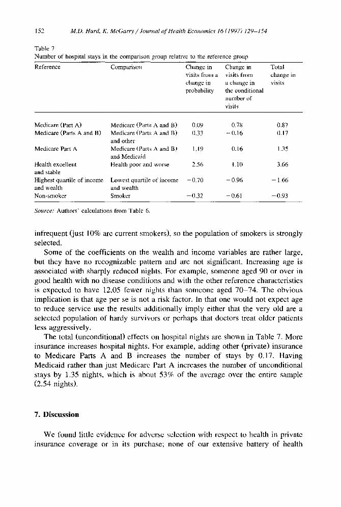
Table 7

Number of hospital stays in the comparison group relative to the reference group

Reference Comparison Change in Change in visits from a visits from

change in a change in probability the conditional

number of

visits

Total

change in visits

Medicare (Part A) Medicare (Parts A and B) 0.09 0+78 0.87 Medicare (Parts A and B) Medicare (Parts A and B) 0.33 - 0.16 0.17

and other

Medicare Part A Medicare (Parts A and B) 1.19 0.16 1.35 and Medicaid

Health excellent Health poor and worse 2.56 1,10 3.66 and stable Highest quartile of income Lowest quartile of income - 0.70 - 0.96 - 1.66 and wealth and wealth

Non-smoker Smoker - 0.32 - 0.61 - 0.93

Source." Authors' calculations from Table 6.

infrequent (just 10% are current smokers), so the population of smokers is strongly selected.

Some of the coefficients on the wealth and income variables are rather large, but they have no recognizable pattern and are not significant. Increasing age is associated with sharply reduced nights. For example, someone aged 90 or over in good health with no disease conditions and with the other reference characteristics is expected to have 12.05 fewer nights than someone aged 70-74. The obvious implication is that age per se is not a risk factor. In that one would not expect age to reduce service use the results additionally imply either that the very old are a selected population of hardy survivors or perhaps that doctors treat older patients less aggressively.

The total (unconditional) effects on hospital nights are shown in Table 7. More insurance increases hospital nights. For example, adding other (private) insurance to Medicare Parts A and B increases the number of stays by 0.17. Having Medicaid rather than just Medicare Part A increases the number of unconditional stays by 1.35 nights, which is about 53% of the average over the entire sample (2.54 nights).

7. Discussion

We found little evidence for adverse selection with respect to health in private insurance coverage or in its purchase; none of our extensive battery of health


conditions had any systematic effect on coverage or purchase. While we cannot rule out the possibility that unobservabte characteristics have a systematic influence on both the propensity to purchase insurance and on service use, in our data the most straightforward explanation of the purchase of supplemental insurance is the economic resources of the individual, not health. On the basis of these findings we interpret the observed relationship between insurance coverage and service use to be the result of the incentives embodied in the insurance, not to any health differences that are systematically related to coverage. Under this interpretation, we can estimate from our results the effects of changing either private or public insurance holdings on service use.

Consider the effect of eliminating private supplemental insurance, as has been advocated as a way to reduce Medicare costs by restoring the incentive effects of the co-payments. In Table 5 we found that moving from Medicare Parts A and B, to Medicare Parts A and B and other, increases the expected number of doctor visits per person by just 0.24. The 7061 Medicare eligible individuals in our sample represent a total population of approximately 21.7 million from the U.S. population. Assuming that 70% of these 21.7 million individuals have private insurance (roughly the fraction of our sample with Medicare and other insurance) yields a population of 15.2 million with both Medicare and other insurance. At 0.24 additional visits per person there are a total of 3.6 million additional doctor visits induced by the supplemental insurance holdings. At an approximate cost to Medicare of $58 per visit, 21 these 'extra visits' cost Medicare $212 million according to our estimates. In the context of the overall cost of the Medicare system this is not a large amount. By comparison, adding Part B of Medicare increases the expected number of visits by 0.93. For the approximately 19.7 million people with Part B of Medicare (91% of 21.7 million), the additional number of office visits is 18.4 million at a cost of $1.07 billion.

Economic status also affects use, particularly doctor visits, both directly and indirectly through greater purchase of private insurance. These findings have a bearing on assessing the redistributive effects of Medicare. The Medicare tax on earnings is a flat tax. The welt-to-do live longer and, if, in addition, they use Medicare more intensively because their supplemental insurance eliminates any co-payments, then they will receive greater lifetime transfers than the poor. Then, the overall effect of Medicare will be regressive.

Acknowledgements

We are grateful to David Cutler, Joseph Newhouse, Kenneth Sokoloff, and an anonymous referee for helpful comments. McGarry 's research was supported by

21 This number is taken by dividing the total amount reimbursed by Medicare Part B for medical services provided by physicians to those age 65 and over, by the number of bills for such services.


NIA grant number T32-AG00186 to the NBER, and by the Brookdale Foundation. Hurd acknowledges financial support from the National Institute on Aging.

References

Eggers, P.W. and R.H. Prihoda, 1982, Pre-enrollment reimbursement: Patterns of Medicare beneficia- ries enrolled in at-risk HMOs, Health Care Financing Review 4, 55-74.

Ettner, S., 1995, Adverse selection and the purchase of medigap insurance by the elderly, paper presented at the 1995 NBER Summer Institute, Cambridge, MA.

Hellinger, F.J., 1995, Selection bias in HMOs and PPOs: A review of the evidence, Inquiry 32, 135-142.

Lillard, L.A. and J. Rogowski, 1995, Does supplemental private insurance increase Medicare costs?, paper presented at the 1995 NBER Summer Institute, Cambridge, MA.

Link, C.R., S.H. Long and R.F. Settle, 1980, Cost sharing, supplementary insurance, and health services utilization among the Medicare elderly, Health Care Financing Review 2, 25-31.

Marquis, M.S. and C.E. Phelps, 1987, Price elasticity and adverse selection in the demand for supplementary health insurance, Economic Inquiry 25, 299-313.

McCall, N., T. Rice, J. Boismier and R. West, 1991~ Private health insurance and medical care utilization: Evidence from the Medicare population, Inquiry 28, 276-287.

Monheit, A.C. and C.L. Schur, 1989, Health insurance coverage of retired persons, DHHS Publication No. 89-3444, National Medical Expenditure Survey Research Findings 2 (National Center for Health Services Research and Health Care Technology Assessment, Rockville, MD).

National Academy on Aging, 1995, Facts on Medicare: Hospital insurance and supplementary Medicare insurance (Baltimore, MD).

Newhouse, J.P., 1996, Reimbursing health plans and health providers: Selection vs. efficiency in production, Journal of Economic Literature, in press.

Newhouse, J.P. and the Insurance Experiment Group, 1993, Free for all? Lessons from the RAND Health Insurance Experiment (Harvard University Press, Cambridge, MA).

Price, J.R. and J.W. Mays, 1985, Biased selection in the Federal Employees Health Benefits Program, Inquiry 22, 67-77.

Physician Payment Review Commission, 1996, Annual Report to Congress (Washington, DC). Rothschild, M. and J. Stiglitz, t976, Equilibrium in competitive insurance markets: An essay on the

economics of imperfect information, Quarterly Journal of Economics 90, 630-649. Smith, J.P., 1995, Wealth inequality among older Americans, Labor and Population Program Working

Paper 95-06, RAND, Santa Monica, CA. U.S. Bureau of the Census, 1993, Statistical abstract of the United States: 1993 (Washington, DC). Wilson, C., 1977, A model of insurance markets with incomplete information, Journal of Economic

Theory 17, 167-207. Wolfe, J.R. and J.H. Goddeeris, 1991, Adverse selection, moral hazard, and wealth effects in the

medigap insurance market, Journal of Health Economics 10, 433-459.

medical insurance and the use of health care services by ... · medical insurance and the use of...

Documents