medium term pasa process description · medium term pasa process description doc ref: 42 v3.0 30...

MEDIUM TERM PASA PROCESS DESCRIPTION

PREPARED BY: Systems Capability

DOCUMENT REF: 42

VERSION: 3.0

DATE: 30 May 2013

FINAL

Australian Energy Market Operator Ltd ABN 94 072 010 327 www.aemo.com.au inlo@oemo .com.au

NEW SOUTH WALES QUEENSLAND SOUTH AUSTRALIA VICTORIA AUSTRALIAN CAPITAL TERRITORY TASMANIA


Doc Ref: 42 v3.0 30 May 2013 of 25

Disclaimer

Purpose

This report has been prepared by the Australian Energy Market Operator Limited (AEMO) for the sole purpose of meeting obligations in accordance with clause 3.7.2(g) of the National Electricity Rules.

No reliance or warranty

This report contains data provided by third parties and might contain conclusions or forecasts and the like that rely on that data. This data might not be free from errors or omissions. While AEMO has used due care and skill, AEMO does not warrant or represent that the data, conclusions, forecasts or other information in this report are accurate, reliable, complete or current or that they are suitable for particular purposes. You should verify and check the accuracy, completeness, reliability and suitability of this report for any use to which you intend to put it, and seek independent expert advice before using it, or any information contained in it.

Limitation of liability

To the extent permitted by law, AEMO and its advisers, consultants and other contributors to this report (or their respective associated companies, businesses, partners, directors, officers or employees) shall not be liable for any errors, omissions, defects or misrepresentations in the information contained in this report, or for any loss or damage suffered by persons who use or rely on such information (including by reason of negligence, negligent misstatement or otherwise). If any law prohibits the exclusion of such liability, AEMO’s liability is limited, at AEMO’s option, to the re-supply of the information, provided that this limitation is permitted by law and is fair and reasonable.

© 2013 Australian Energy Market Operator Ltd. All rights reserved

Glossary

ABBREVIATION ABBREVIATION EXPLANATION

AEMO Australian Energy Market Operator

AWEFS Australian Wind Energy Forecasting System

ESOO Electricity Statement of Opportunities

LOR Lack of Reserve Level

LOR1: Lack of Reserve Level 1



LP Linear Program

LRC Low Reserve Condition

MMS Electricity Market Management System

MNSP Market Network Service Provider (Scheduled Network Service Provider in the National Electricity Rules)

MRL Minimum Reserve Level

Native demand The electricity demand met by scheduled, semi-scheduled, non-scheduled and exempt generation.


Doc Ref: 42 v3.0 30 May 2013 of 25

NEM National Electricity Market

NEFR National Electricity Forecasting Report

Rules National Electricity Rules (the Rules)

PASA Projected Assessment of System Adequacy

ST PASA: Short term projected assessment of system adequacy

MT PASA: Medium term projected assessment of system adequacy

POE Probability of Exceedence

RHS Right Hand Side of a constraint equation

Timetable Spot Market Operations Timetable

UIGF Unconstrained Intermittent Generation Forecast


Doc Ref: 42 v3.0 30 May 2013 of 25

Contents

Introduction ...................................................................................................... 6 1

MT PASA process and Rules requirements ..................................................... 7 2

MT PASA Inputs ............................................................................................... 8 3

3.1 Market participant inputs ............................................................................................ 8

3.1.1 Generating unit availabilities for MT PASA ................................................................................. 8 3.1.2 Network outages and Interconnector availabilities ...................................................................... 9

3.2 AEMO inputs .............................................................................................................. 9

3.2.1 Plant availabilities for MT PASA .................................................................................................. 9 3.2.2 Demand forecasts ..................................................................................................................... 10 3.2.3 Minimum Reserve Levels .......................................................................................................... 11 3.2.4 Power transfer capabilities used in MT PASA .......................................................................... 11

MT PASA Solution Process ............................................................................12 4

4.1 Reliability LRC (RELIABILITY_LRC) ........................................................................ 12

4.2 Regional Reliability MSR MUR (RELIABILITY_MSR_MUR) ..................................... 12

4.3 Regional Lack of Reserve (LOR): ............................................................................. 13

4.4 Modelling of Inter-regional Reserve Sharing in MT PASA Solution Process ............. 13

MT PASA Outputs ...........................................................................................14 5

Appendix A: MT PASA Process Architecture ...............................................................17

Appendix B: Medium Term Demand Forecasting Process ..........................................18

Appendix C: Reserve Sharing Example .......................................................................21

Appendix D: Pain Sharing Example .............................................................................21

Appendix E: Formulae for Reserve Calculations in RLRC, OLRC and LOR solves .....22

Appendix F: Lack of Reserve (LOR) Condition Calculation .........................................23


Doc Ref: 42 v3.0 30 May 2013 of 25

Version Release History

VERSION DATE BY CHANGES

1.0 27/04/2006 SOPP Initial version

2.0 22/03/2013 Systems Capability

Review document to reflect current processes

3.0 30/05/2013 Systems Capability

Updated Sections 4, 5 and Appendix E to include new runtype RELIABILITY_MSR_MUR, reporting of MaxUsefulResponse (MUR) and four new runtypes associated with interconnector capability reporting.


Doc Ref: 42 v3.0 30 May 2013 of 25

Introduction 1

The National Electricity Rules (the Rules) clause 3.7.1 requires Australian Energy Market Operator (AEMO) to administer the projected assessment of system adequacy (PASA) processes.

The PASA is the principal method of indicating to the National Electricity Market (NEM) a forecast of power system security and supply reliability of electricity for a period of up to 2 years. The Rules require AEMO to administer the PASA for two timeframes:

1. Medium Term PASA (MT PASA) which covers a 24 month period commencing from the Sunday after the day of publication with a daily resolution; and

2. Short Term PASA (ST PASA) which covers a period of six trading days starting from the end of the trading day covered by the most recently published pre-dispatch schedule with a trading interval resolution.

The MT PASA assesses the power system security and reliability under 10% Probability of Exceedence (POE) and 50% POE demand conditions based on generator availabilities submitted by market participants with due consideration to planned transmission outages.

The MT PASA has the following objectives:

Provide sufficient information on the expected level of medium term capacity reserve and hence allow market participants to schedule planned outages of generating units.

Alert the market of any days on which low reserve condition (LRC) or lack of reserve (LOR) are forecast to occur.

Provide a basis for AEMO to intervene in the market (i.e. Reserve Trading process1) through the Reliability and Emergency Reserve Trader provisions as per clause 3.20 of the Rules.

The MT PASA process is administered according to the timeline set out in the Spot Market Operations Timetable2 (timetable) in accordance with the Rules.

This document is intended to fulfil AEMO’s obligation under clause 3.7.2(g) of the Rules to document the procedure used in administering the MT PASA.

1 http://www.aemo.com.au/Electricity/Market-Operations/Reserve-Management

2 http://www.aemo.com.au/Electricity/Market-Operations/Dispatch/Spot-Market-Operations-Timetable

http://www.aemo.com.au/Electricity/Market-Operations/Reserve-Management

http://www.aemo.com.au/Electricity/Market-Operations/Dispatch/Spot-Market-Operations-Timetable


Doc Ref: 42 v3.0 30 May 2013 of 25

MT PASA process and Rules requirements 2

The PASA is a comprehensive program for the collection and analysis of information in order to assess the medium term and short term power system security and reliability of supply prospects.

The assessment of medium term power system security and reliability in the MT PASA process is based on comparing the medium term capacity reserves available against the required levels determined in the Reliability Standard.

Medium term capacity reserve, as defined by the Rules, is the aggregate amount of generating capacity indicated by the relevant Generators as being available any time on a particular day during the period covered by the medium term PASA, and which is assessed by AEMO as being in excess of the capacity requirement to meet the forecast peak load, taking into account the known or historical levels of demand management.

The objective of the PASA is to provide projected system reserve conditions, and projected regional reserve conditions to market participants in the MT PASA timeframe along with additional information including forecast demand, expected aggregate plant capacity.

Clause 3.7.2 of the Rules details the requirements for the administration of the MT PASA.

Under this Rules clause, AEMO must review and publish the outputs of the MT PASA every week, covering the 24 month period commencing from the Sunday after the day of publication with a daily resolution. Additional updated versions of the MT PASA may be published by AEMO in the event of changes which, in the judgement of AEMO, are materially significant and should be communicated to Registered Participants.

The responsibilities of each party in the preparation of the MT PASA (summarised in Table 1 below) are also defined in this clause.

Table 1: Rules requirements

Responsible Party Action Rules Requirement

AEMO Prepare following MT PASA inputs:

Regional demand forecasts

Reserve requirements

Network constraints forecasts

Unconstrained intermittent generation forecasts for semi-scheduled generating unit

3.7.2(c)

Scheduled Generator or Market Participant

Submit to AEMO the following MT PASA inputs:

PASA availability of each scheduled generating unit, scheduled load or scheduled network service

Weekly energy constraints applying to each scheduled generating unit or scheduled load

3.7.2(d)

Network Service Providers

Provide AEMO the following information:

Outline of planned network outages

Any other information on planned network outages that is reasonably requested by AEMO

3.7.2(e)

AEMO Prepare and publish the MT PASA outputs 3.7.2(f)


Doc Ref: 42 v3.0 30 May 2013 of 25

MT PASA Inputs 3

Inputs used in the MT PASA process are provided by both AEMO and market participants. They are discussed in detail below.

3.1 Market participant inputs

Market participants are required to submit the following data covering a 24 month period from the Sunday after the day of publication of the MT PASA

3.1.1 Generating unit availabilities for MT PASA

Generating unit PASA availabilities:

MT PASA uses PASA Availabilities of generating units. PASA availability includes the generating capacity in services as well as the generating capacity that can be delivered with 24 hours’ notice.

As per clause 3.7.2(d)(1), Generators are required to provide the expected MW capacity of each scheduled generating unit or scheduled load on a daily basis for the next 2 years. The actual level of generation available at any particular time will depend on the condition of the generating plant, which includes factors such as age, outages, and wear. Another important factor with respect to output is the reduction in thermal efficiency with increasing temperature3.

Generators should take into account the ambient weather conditions expected at the time when the Region where the generating unit is located experiences the 10% Probability of Exceedence (POE) peak load defined as Generation Capacity Reference Temperatures. The summer and winter AEMO generation capacity reference temperature for each region are available in the Background Information worksheet of the Generator Information spreadsheet for each region published on the AEMO website4.

Generating unit energy availabilities:

Generating plant such as hydroelectric power stations cannot generally operate at maximum capacity indefinitely due to the possibility of their energy source being exhausted. Under clause 3.7.2(d)(2) scheduled generating units with energy constraints (referred to as energy constrained plant) are required to submit their weekly energy limit in MWh for each week for the upcoming 24 month period commencing from the first Sunday after the latest MT PASA run. The energy constrained plant5 are allocated accordingly to the ratio of the forecast demand to the PASA availabilities, i.e. more energy is located to period when the ratio of the forecast demand to the PASA availabilities is high.

For MT PASA to be able to allocate the energy constrained plants, it requires information on expected demand and its profile as well as PASA availabilities on any given day.

Wind turbine availabilities:

To facilitate AEMO to fulfil its obligation in producing semi-scheduled generating unit forecasts as per clause 3.7.2(c)(4), participants who own such units are required to submit wind turbine availability information to AEMO. Based on this information, semi-scheduled

3 http://www.aemo.com.au/Electricity/Planning/Related-Information/Generation-Information

4 Generation capacity reference temperatures are available at:

http://www.aemo.com.au/Electricity/Planning/Related-Information/Generation-Information

5 The capacity of all energy constrained plants within each region is reported as CONSTRAINEDCAPACITY and the

capacity of all generating plants that are not limited by energy within each region are reported as UNCONSTRAINEDCAPACITY in the MTPASA.RegionSolution table. A guide to the information contained in the MT PASA is available in the form of a data model at http://www.aemo.com.au/Electricity/Resources/Information-Systems/Market-Management-System-Data-Model



http://www.aemo.com.au/Electricity/Resources/Information-Systems/Market-Management-System-Data-Model



Doc Ref: 42 v3.0 30 May 2013 of 25

wind forecast profiles are developed by AEMO. This is discussed in more detail in section 3.2.1.

3.1.2 Network outages and Interconnector availabilities

Under clause 3.7.2(e), Network Service Providers must provide to AEMO an outline of planned network outages and any other information on planned network outages that is reasonably requested by AEMO. This includes interconnector availability information (e.g. Basslink). The planned network outages are converted into network constraints by AEMO. This process is further discussed in Section 3.2.4.

3.2 AEMO inputs

3.2.1 Plant availabilities for MT PASA

In addition to the plant availability information provided by market participants as discussed in the earlier section, AEMO also prepares the following data as part of the plant availabilities.

Semi-scheduled wind generation forecasts:

AEMO is required to produce an unconstrained intermittent generation forecast (UIGF) for each semi-scheduled generating unit for each day in accordance to clause 3.7.2(c)(4).

The UIGF is the equivalent forecast of electrical power output from an intermittent generating unit (or intermittent generating system, if aggregated under clause 3.8.3 of the Rules) based on the forecast amount of raw energy available for conversion into electrical power, as limited by the available generating capacity of that generating facility. This generation forecast is “unconstrained” in the sense that it is based on the raw energy input to the unit’s power conversion process and ignores overriding factors that are external to the power conversion process, such as the impact of any network constraint on the output or any economic requirement to otherwise operate at reduced levels.

The process taken by AEMO to generate semi-scheduled wind generation forecasts is shown in figure 1 below, in which the Australian Wind Energy Forecasting System (AWEFS) model is used as the forecasting tool.

AEMO Inputs

Historical data

(wind/temperature)

Generator Inputs

Turbine availabilities

AWEFS modelSemi-scheduled generating

unit forecasts

Figure 1: Semi-scheduled generating unit (wind farm) forecasts

Non-scheduled generation forecasts:

In accordance to clause 3.7.2(f)(2), AEMO is required to prepare and publish the aggregated MW allowance (if any) to be made by AEMO for generation from non-scheduled generating systems.

The non-scheduled generation profiles constitute of two components: non-scheduled wind generation and other non-scheduled generation. The non-scheduled wind generation


Doc Ref: 42 v3.0 30 May 2013 of 25

forecasts6 are produced in a similar way to the semi-scheduled wind generation while the other non-scheduled generation forecasts are consistent with figures published in the Electricity Statement of Opportunities (ESOO)7.

The non-scheduled generation forecasts are used as an input to MT PASA demand forecasting process. This is discussed in more detail in Section 3.2.2.

Demand Side Participation (DSP):

DSP includes all short-term reductions in demand in response to temporary price increases (in the case of retailers and customers) or adverse network loading conditions (in the case of networks). An organised, aggregated response may also be possible. From the perspective of the transmission network, consumers may effectively reduce demand by turning off electricity-using equipment or starting up on-site generators.

AEMO conducted a survey of stakeholders to ascertain potential DSP sites and future DSP opportunities. The results of the survey form the basis of AEMO’s regional estimates of historical and projected DSP. This information is published in the ESOO.

The MT PASA uses the ESOO’s seasonal DSP forecasts of medium growth.

Future generation:

Committed generation projects currently under development with a dispatch type of scheduled or semi-scheduled are also modelled in MT PASA.

Before the unit is registered, it is modelled as future generation which has the PASA availabilities as its seasonal capacity and is available from the start date of commercial operation. This information is obtained from the ESOO, and subsequent updates are obtained from Generators. Once the unit is registered, the Generator that owns the unit is responsible for submitting unit offer data to AEMO and the unit is modelled similarly to other existing generations.

3.2.2 Demand forecasts

For the MT PASA, AEMO prepares a forecast of electricity maximum demand for each region for each day based on the peak demand forecasts from the National Electricity Forecasting Report8 and historical patterns of electricity used, allowing for factors such as seasons, day of the week and public holidays, as per clause 3.7.2(c)(1).

The actual demand differs from the forecast (mainly due to weather changes) usually randomly. Statistically, it can be assumed that the forecast error follows a normal distribution. Accordingly, a forecast can be qualified by the probability that the actual demand will exceed the forecast demand, or POE.

A 10% POE forecast9 indicates that there is a 10% chance that the actual demand will exceed the forecast value (i.e. Peak demand will be exceeded once in 10 years).

A 50% POE forecast indicates that there is a 50% chance that actual demand will exceed the forecast value.

Refer to Appendix B for further information on the derivation of MT PASA demand forecasts.

6 The non-scheduled wind generation forecasts are reported as TOTALINTERMITTENTGENERATION in the

MTPASA.RegionSolution table. A guide to the information contained in the MT PASA is available in the form of a data

model at http://www.aemo.com.au/Electricity/Resources/Information-Systems/Market-Management-System-Data-Model 7 http://www.aemo.com.au/Electricity/Planning/Electricity-Statement-of-Opportunities

8 http://www.aemo.com.au/AEMO%20Home/Electricity/Planning/Forecasting

9The 10% POE and 50% POE Demand forecasts are reported as DEMAND10 and DEMAND50 in the

MTPASA.RegionSolution table. A guide to the information contained in the MT PASA is available in the form of a data

model at http://www.aemo.com.au/Electricity/Resources/Information-Systems/Market-Management-System-Data-Model


http://www.aemo.com.au/Electricity/Planning/Electricity-Statement-of-Opportunities

http://www.aemo.com.au/AEMO%20Home/Electricity/Planning/Forecasting



Doc Ref: 42 v3.0 30 May 2013 of 25

3.2.3 Minimum Reserve Levels

Under the Reliability Standard, the NEM should aim to achieve an expected unserved energy (USE) of no more than 0.002% in each financial year, each region and in the NEM as a whole. AEMO is required to determine reserve requirement for each region in accordance with the medium term capacity reserve standards as per clause 3.7.2(c)(2).

The Minimum Reserve Level (MRL) that is used in MT PASA for each region is derived off-line from a series of probabilistic Monte-Carlo studies that aim to determine the minimum local generation required in each region to target 0.002% USE in all regions. In other words, the USE Reliability Standard is translated into operational trigger in the form of MRL equations.

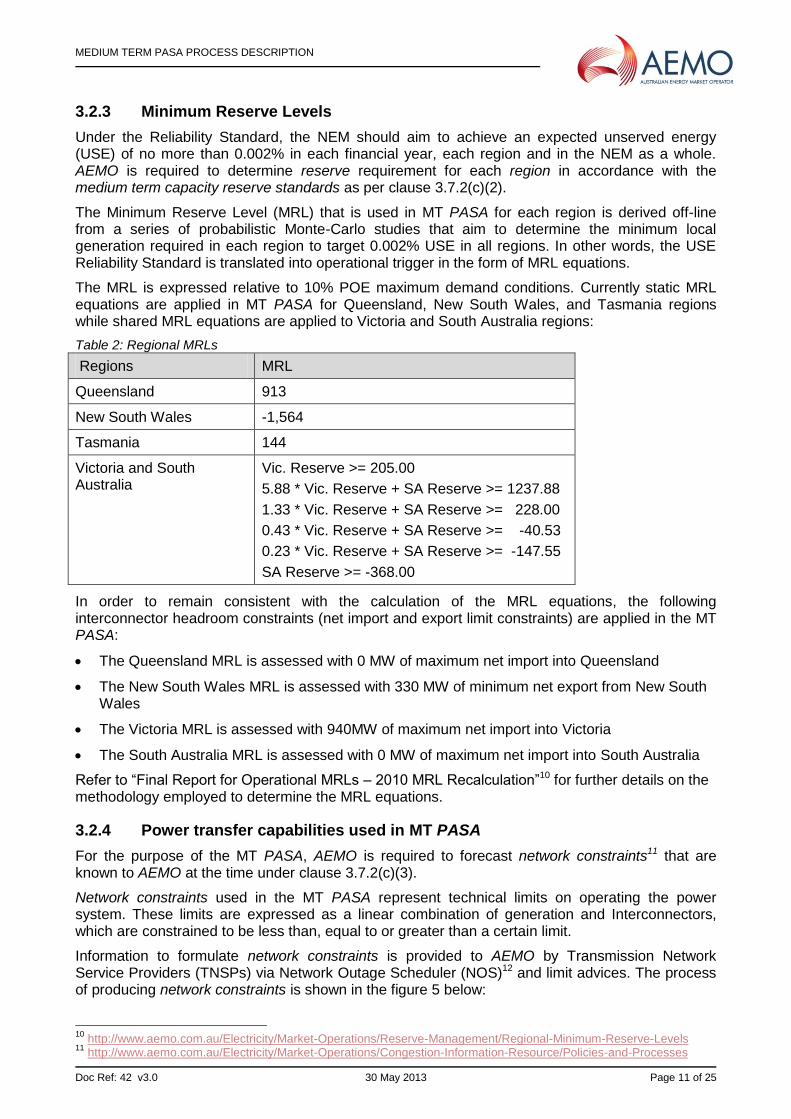
The MRL is expressed relative to 10% POE maximum demand conditions. Currently static MRL equations are applied in MT PASA for Queensland, New South Wales, and Tasmania regions while shared MRL equations are applied to Victoria and South Australia regions:

Table 2: Regional MRLs

Regions MRL

Queensland 913

New South Wales -1,564

Tasmania 144

Victoria and South Australia

Vic. Reserve >= 205.00

5.88 * Vic. Reserve + SA Reserve >= 1237.88

1.33 * Vic. Reserve + SA Reserve >= 228.00

0.43 * Vic. Reserve + SA Reserve >= -40.53

0.23 * Vic. Reserve + SA Reserve >= -147.55

SA Reserve >= -368.00

In order to remain consistent with the calculation of the MRL equations, the following interconnector headroom constraints (net import and export limit constraints) are applied in the MT PASA:

The Queensland MRL is assessed with 0 MW of maximum net import into Queensland

The New South Wales MRL is assessed with 330 MW of minimum net export from New South Wales

The Victoria MRL is assessed with 940MW of maximum net import into Victoria

The South Australia MRL is assessed with 0 MW of maximum net import into South Australia

Refer to “Final Report for Operational MRLs – 2010 MRL Recalculation”10 for further details on the methodology employed to determine the MRL equations.

3.2.4 Power transfer capabilities used in MT PASA

For the purpose of the MT PASA, AEMO is required to forecast network constraints11 that are known to AEMO at the time under clause 3.7.2(c)(3).

Network constraints used in the MT PASA represent technical limits on operating the power system. These limits are expressed as a linear combination of generation and Interconnectors, which are constrained to be less than, equal to or greater than a certain limit.

Information to formulate network constraints is provided to AEMO by Transmission Network Service Providers (TNSPs) via Network Outage Scheduler (NOS)12 and limit advices. The process of producing network constraints is shown in the figure 5 below:

10

http://www.aemo.com.au/Electricity/Market-Operations/Reserve-Management/Regional-Minimum-Reserve-Levels 11

http://www.aemo.com.au/Electricity/Market-Operations/Congestion-Information-Resource/Policies-and-Processes

http://www.aemo.com.au/Electricity/Market-Operations/Reserve-Management/Regional-Minimum-Reserve-Levels

http://www.aemo.com.au/Electricity/Market-Operations/Congestion-Information-Resource/Policies-and-Processes


Doc Ref: 42 v3.0 30 May 2013 of 25

TNSPs

Network outage schedule Network constraints

AEMO

Limit advices

Network Outage Scheduler

Figure 2: Formulation of network constraints

Within AEMO’s market systems, constraints can be marked as system normal (i.e. power system constraints that assume all plants are in service). Alternatively, to model network or plant outage in the power system, separate outage constraints are formulated and applied along with system normal constraints. This will be further discussed in section 4.

MT PASA Solution Process 4

In order to assess system adequacy, the MT PASA performs three groups of Linear Programming (LP) runs to identify low reserve conditions (LRC) or lack of reserve conditions (LOR) in NEM regions:

4.1 Reliability LRC (RELIABILITY_LRC)

This run assesses whether the medium term capacity reserves in NEM over the MT PASA period is adequate. For this assessment a Capacity Adequacy LP model is used.

Capacity Adequacy LP model:

This model maximises spare generation capacity (MT PASA considers scheduled and semi-scheduled generation only) in NEM above the summation of 10% POE regional demand forecasts and regional minimum reserve requirements subjected to:

PASA Availability of generation and weekly energy limits (includes committed future generation)

Power transfer capability of the power system with no planned network outages

Where medium term capacity reserves do not meet the required level, the deficit is shared on a pro-rata basis among regions subject to applicable interconnector constraints. Reporting reserve deficits shared on a pro-rata basis is referred to as “Pain Sharing”. Refer Appendix D for an example of the application of Pain Sharing.

The outcome of the Reliability LRC run is an indication of the supply reliability in NEM over the MT PASA period and is used as a key input to trigger Reliability and Emergency Reserve Trader (RERT) process as required by the Rules Clause 3.2013.

4.2 Regional Reliability MSR MUR (RELIABILITY_MSR_MUR)

This run uses the same inputs as the Reliability LRC run (10% POE Demand, PASA Availability and energy limitations with no network outages). The purpose of this run is to report the Maximum Useful Response (MUR) and Maximum Surplus Reserve (MSR) assessments based on 10% POE Demand and system normal conditions. Maximum Useful Response (MUR) and Maximum Surplus Reserve (MSR) assessments are detailed below:

(a) Regional Maximum Useful Response (MUR) LP model:

The MUR LP model determines the maximum MW contribution from each region useful to relieve a reserve deficit reported in the Regional Reliability LRC (RELIABILITY_LRC) Capacity Adequacy

12

http://nos.prod.nemnet.net.au/nos 13

Procedure for the Exercise of Reliability and Emergency reserve Trader is available at: http://www.aemo.com.au/Consultations/National-Electricity-Market/Closed/Procedure-for-the-Exercise-of-Reliability-and-Emergency-Reserve-Trader-RERT-Consultation

http://nos.prod.nemnet.net.au/nos

http://www.aemo.com.au/Consultations/National-Electricity-Market/Closed/Procedure-for-the-Exercise-of-Reliability-and-Emergency-Reserve-Trader-RERT-Consultation

http://www.aemo.com.au/Consultations/National-Electricity-Market/Closed/Procedure-for-the-Exercise-of-Reliability-and-Emergency-Reserve-Trader-RERT-Consultation


Doc Ref: 42 v3.0 30 May 2013 of 25

run defined in Section 4.1. MUR determines useful contribution from each NEM region by running this model multiple times, taking each region as the study region in turn.

(b) Regional Maximum Surplus Reserve (MSR) LP model:

The MSR model determines the maximum generation that can be withdrawn from a region without causing a Low Reserve Condition (LRC) in any of the NEM regions. MSR determines the maximum generation that can be withdrawn from each NEM region by running this model multiple times, taking each region as the study region in turn.

4.3 Regional Lack of Reserve (LOR):

This model maximises spare generation in NEM regions above their 50% POE regional demand forecasts subjected to:

PASA availability of generation and weekly energy limits (includes committed future generation)

Power transfer capability of the power system taking planned network outages into account

MSC run determines spare generation capacity in each NEM region by running this model multiple times, taking each region as the study region in turn.

Table 3 provides a summary of the sets of inputs and linear programming (LP) models used in performing the three runs as well as their outputs.

A brief description of the architecture of the MT PASA program is provided in Appendix A.

Simplified examples to illustrate methodology behind Maximum Spare Capacity calculation in LOR runs is provided in Appendix F.

4.4 Modelling of Inter-regional Reserve Sharing in MT PASA Solution Process

CA models

When the total generation capacity of a region is greater than required for that region, the spare capacity can be shared with adjacent regions in order to meet reserves requirements of other regions, provided that the interconnectors flow14 limits is not exceeded. This is referred to as reserve sharing.

The inter-regional power transfers are modelled in Capacity Adequacy models used in Reliability LRC run such that the inter-regional power transfers (reserve sharing) take place only to minimise reserve shortfalls in NEM regions.

An example illustrating the reserve sharing principle is shown in Appendix C.

MUR, MSR and MSC models

These models accommodate inter-regional power transfers (reserve sharing) to maximise reserves/spare capacity in the study region after meeting the reserve requirements/supply demand balance in other regions.

14 The net interconnector flow into a region in the Reliability LRC run is reported as

NETINTERCHANGEUNDERSCARCITY in the MTPASA.RegionSolution table. The net interconnector flow into a region in the MSR and MUR solves of RELIABILITY_MSR_MUR run is reported as MSRNETINTERCHANGEUNDERSCARCITY and MURNETINTERCHANGEUNDERSCARCITY in the MTPASA.RegionSolution table. A guide to the information contained in the MT PASA is available in the form of a data model at http://www.aemo.com.au/Electricity/Resources/Information-Systems/Market-Management-System-Data-Model



Doc Ref: 42 v3.0 30 May 2013 of 25

MT PASA Outputs 5

Under clause 3.7.2(f) of the Rules, AEMO must publish the MT PASA outputs as part of the MT PASA process15. The main output from MT PASA is the forecast of any low reserve condition16 or lack of reserve conditions.

If capacity reserves are forecast to fall below reference levels, AEMO may declare the following conditions in the MT PASA. These are defined in clause 4.8.4 of the Rules and applied as follows:

Low Reserve Condition (LRC)17 - When the medium term capacity reserves available in a region is forecast to be less than the medium term capacity reserve standard for that region.

Lack of reserve level 1 (LOR1) - When the medium term capacity reserves available in a region is forecast to be less than the sum of the largest and the second largest generation losses due to a credible contingency event in that region.

Lack of reserve level 2 (LOR2) - When the medium term capacity reserves available in a region is forecast to be less than the largest generation loss due to a credible contingency event in that region.

Lack of reserve level 3 (LOR3) - When involuntary load shedding is forecast due to supply shortage.

The Low reserve condition for a region is reported as RESERVECONDITION in the MTPASA.RegionSolution table. Appendix E lists formulae used in the calculation of the above quantities.

Under clause 3.7.2 (6) (iv) of the Rules, AEMO must publish forecast interconnector transfer capabilities as part of the MT PASA process. For the publication of the interconnector transfer capabilities under different demand and system conditions, four new runs namely, RELIABILITY_LIMITS, OUTAGE_LIMITS, RELIABILITY_LOR and OUTAGE_LOR have been introduced in the MT PASA process. The LP solves used in determining the interconnector limits are the existing Capacity Adequacy (CA) and Max Spare Capacity (MSC) solves used in the Regional Reliability LRC (Section 4.1) and Regional LOR (Section 4.3) runs. Table 4 provides a summary of the sets of inputs and linear programming (LP) models used in performing the four runs as well as their outputs.

15

http://www.nemweb.com.au/REPORTS/CURRENT/MEDIUM_TERM_PASA_REPORTS/. A guide to the information contained in the MT PASA is available in the form of a data model at

http://www.aemo.com.au/Electricity/Resources/Information-Systems/Market-Management-System-Data-Model 16

http://www.aemo.com.au/Electricity/Data/Forecast-Supply-and-Demand/Medium-Term-Outlook 17

The Low reserve condition and Lack of Reserve Levels for each region is reported as RESERVECONDITION and LORCONDITION respectively in the MTPASA.RegionSolution table. A guide to the information contained in the MT PASA is available in the form of a data model at http://www.aemo.com.au/Electricity/Resources/Information-Systems/Market-Management-System-Data-Model

http://www.nemweb.com.au/REPORTS/CURRENT/MEDIUM_TERM_PASA_REPORTS/


http://www.aemo.com.au/Electricity/Data/Forecast-Supply-and-Demand/Medium-Term-Outlook




Doc Ref: 42 v3.0 30 May 2013 of 25

Table 3: Summary of the three MT PASA run types in system adequacy assessment

Reliability LRC (RELIABILITY_LRC) Regional Reliability MSR MUR (RELIABILITY_MSR_MUR)

Regional LOR

Inpu

ts C

om

mo

n I

nputs

Reserve requirement

PASA availabilities

Unit energy availabilities

Non-scheduled generation forecasts

DSP forecasts

Future generation forecasts

Diffe

rent In

pu

ts

10% POE demand forecasts

System normal constraints with the RHS using 10% POE demand for region terms and PASA unit availabilities for trader term

10% POE semi-scheduled generation forecasts

Full availability of interconnectors

50% POE demand forecasts

System normal constraints and outage constraints with the RHS using 50% POE demand for region terms and PASA unit

availabilities for trader term

50% POE semi-scheduled generation forecasts

Taken into account any interconnector outages

LP

mo

de

l

Capacity Adequacy run Maximum Useful Response (MUR) runs and Max Surplus Reserve (MSR) runs

Max Spare Capacity (MSC) runs

Ou

tputs

Forecasts of low reserve conditions

Forecasts of the most probable peak demand plus required reserve for each NEM region

Aggregate generation that is subjected to energy limits in each forecast of the peak demand

Forecasts of interconnector transfer capability with no outages

Constraints used in the MT PASA solutions which may become binding on the dispatch of generation or load

Forecasts of the maximum MW contribution from each region useful to relieve a low reserve condition reported in the Regional Reliability LRC run. This is reported as Maximum Useful Response (MUR).

Forecasts of the maximum generation that can be withdrawn from a region without causing a low reserve condition in any of the NEM regions. This is reported as Maximum Surplus Reserve (MSR).

Forecasts of Net Interchange into a region under system normal conditions, for MUR and MSR solve.

Forecasts of any lack of reserve conditions

Forecasts of the most probable peak demand plus required reserve for each NEM region

Aggregate generation that is subjected to energy limits in each forecast of the peak demand

Forecasts of interconnector transfer capability with outages

Constraints used in the MT PASA solutions which may become binding on the dispatch of generation or load


Doc Ref: 42 v3.0 30 May 2013 of 25

Table 4: Summary of the four MT PASA run types in interconnector capability assessment

RELIABILITY_LIMITS OUTAGE_LIMITS RELIABILITY_LOR OUTAGE_LOR

Inpu

ts

10% POE Demand



10% POE Demand

System normal constraints and outage constraints with the RHS using 10% POE demand for region terms and PASA unit availabilities for trader term


50% POE Demand



50% POE Demand

System normal constraints and outage constraints with the RHS using 50% POE demand for region terms and PASA unit availabilities for trader term


LP

mo

de

l

Capacity Adequacy (CA) Capacity Adequacy (CA) Max Spare Capacity (MSC)

Max Spare Capacity (MSC)

Ou

tputs

Forecast export limit for all interconnectors under 10% POE demand and system normal conditions.

Forecast import limit for all interconnectors under 10% POE demand and system normal conditions.

Forecast export limit for all interconnectors under 10% POE demand and network outage conditions.

Forecast import limit for all interconnectors under 10% POE demand and and network outage conditions.

Forecast maximum export limit (of all study regions) for all interconnectors under 50% POE demand and system normal conditions.

Forecast minimum import limit (of all study regions) for all interconnectors under 50% POE demand and system normal conditions.

Forecast maximum export limit (of all study regions) for all interconnectors under 50% POE demand and network outage conditions.

Forecast minimum import limit (of all study regions) for all interconnectors under 50% POE demand and network outage conditions.


Doc Ref: 42 v3.0 30 May 2013 of 25

Appendix A: MT PASA Process Architecture

NEMDB

Run Process (CORE PASA SUITE)

PASA SolverPASA Solution

Loader

MT PASA Case

Loader

Data Interchange

(NEMReports)

Participant Systems

EMMS Data

Model

Spreadsheet

Viewers

Run Initiation

SOMMS

AWEFS

(Semi-scheduled

Units)

PASA Solution

Data Server

Public Website

MT PASA Graphs

Offers

MT PASA Offer

Server

EMMSWeb

AEMO Solution

Viewer (internal)

Figure A.1: Architecture of the MT PASA program

The MT PASA process operates as follows as described in figure A.1 above:

1. The valid Registered Participant bid files are loaded into tables in the central Market Management System (MMS) Database. Bid acknowledgments are returned to Registered Participants.

2. All relevant input data is consolidated into a single file for the MT PASA solver.

3. The MT PASA solver sets up various linear constraints based on the input data and runs several linear programs.

4. The MT PASA solver produces an output file which is transferred to the National Electricity Market (NEM) database.

5. A public MT PASA file is created from the input and solution files from the MT PASA solver.

6. The new public MT PASA files are reformatted and sent to each registered participant.


Doc Ref: 42 v3.0 30 May 2013 of 25

Appendix B: Medium Term Demand Forecasting Process

Figure B1 shows the relationship between the regional native demand published in the National Electricity Forecasting Report (NEFR) and the demand used in the MT PASA process. As shown in the figure, the MT PASA uses the demand met by scheduled and semi-scheduled generation.

Demand met by

Scheduled generation

Demand met by

Semi-scheduled

Wind

Demand met by Non-scheduled

Wind

- &

AEMO will

use ESOO

estimate

ESOO Native

Demand Supplied by Other Non Scheduled

Exempt Gen

AEMO will

use AWEFS

forecast

used in MT

PASA

Figure B.1: Various demand components constituting Native Demand

Developing MT PASA demand forecasts consists of two steps:

Step 1 – Derive regional daily peak native demand profiles using NEFR native summer/winter demand as the basis

Step 2 – Derive regional daily peak demand profiles for MT PASA by subtracting the demand met by non-scheduled and exempt generation form the regional daily native peak demand profiles

Following sections explain the method of performing the above two steps.


Doc Ref: 42 v3.0 30 May 2013 of 25

Weekly factor profile

Weekday factor profile

ESOO Native winter/summer

peak demand

(10% and 50% POE – Medium

growth)

Regional public holidays

Regional daily peak demand met by

scheduled and semi-scheduled

generation

(10% and 50% POE)

Regional daily Native

peak demand

(10% and 50% POE)

AWEFS latest daily

forecasts for non-

scheduled wind

ESOO regional daily

forecasts for other non-

scheduled generation

-

-

+

STEP 1

STEP 2

Figure B.2: Method of developing MT PASA demand forecasts

In figure B.2 the weekly factor profile represents a normalised set of factors (i.e. one factor for each week in the year) determined by taking the ratios of actual maximum weekly demand to the seasonal demand published in NEFR for the given historical year. They are derived taking historical demand and temperature data into consideration. Refer figure B.3 below. Note that AEMO uses historical data for past ten years for these steps.

Historical regional

daily peak

demand data

Weekly factor profile

Historical regional

daily maximum/

minimum

temperature

Figure B.3: Development of weekly factor profile

The weekday factor profile referred to in figure B.4 represents the ratios of daily maximum demand to the maximum demand of each week in a year. Weekday factors are derived taking historical daily peak demand data as well as regional public holidays for the last ten years into consideration. The weekday factors are used consistently across all weeks of the forecast period when MT PASA demand forecasts are produced.

Weekday factor profile

Historical regional

daily peak

demand data

Figure B.4: Development of weekday factor profile

Step 2 (refer Figure B.2) consists of deriving the regional 10% POE and 50% POE daily peak demand profiles met by scheduled and semi-scheduled generations.

MT PASA regional 10% POE daily peak demand =


Doc Ref: 42 v3.0 30 May 2013 of 25

Regional 10% POE daily native peak demand

- the most recent daily forecasts of non-scheduled regional wind generation produced by AWEFS (90% POE forecast)

- regional daily forecast profiles of demand supplied by other non-scheduled generation published in ESOO (Medium growth scenario)

MT PASA regional 50% POE daily peak demand =

Regional 50% POE daily native peak demand

- the most recent daily forecasts of non-scheduled regional wind generation produced by AWEFS (50% POE forecast)

- regional daily forecast profiles of demand supplied by other non-scheduled generation published in ESOO (Medium growth scenario)


Doc Ref: 42 v3.0 30 May 2013 of 25

Appendix C: Reserve Sharing Example

In the example shown below, 100 MW of surplus capacity in Region 2 is supplied over the interconnector to meet the deficit capacity in Region 1. This still leaves a reserve shortfall of 200 MW in Region 1. Since the flow on the interconnector has reached its limit, no further capacity can be allocated to Region 1 from Region 2 to reduce its deficit.

Figure C.1: Reserve sharing example

Appendix D: Pain Sharing Example

In the example shown below, the surplus capacity in Region 2 is supplied over the Interconnector to meet the deficit capacity in Region 1. The deficit is reported in proportion to each region’s demand and subject to interconnectors’ limits. This leaves a reserve shortfall of 33 MW in Region 1 and 167 MW in Region 2.

Figure D.1: Pain sharing example


Doc Ref: 42 v3.0 30 May 2013 of 25

Appendix E: Formulae for Reserve Calculations in RELIABILITY_LRC, RELIABILITY_MSR_MUR and LOR solves

Table E.1 below provides the formulae used in deriving the regional reserve data in the different LP solves:

Table E.1: Formulae for reserve calculations

Data Field Run Type Formula

SURPLUSCAPACITY RELIABILITY_LRC UNCONSTRAINEDCAPACITY +

CONSTRAINEDCAPACITY -NETINTERCHANGEUNDERSCARCITY

18 – DEMAND10

DEFICITRESERVE

RELIABILITY_LRC - Min { 0, UNCONSTRAINEDCAPACITY + CONSTRAINEDCAPACITY - NETINTERCHANGEUNDERSCARCITY –

(DEMAND10 + MRL19

)}

RESERVECONDITION

RELIABILITY_LRC

If DEFICITRESERVE > 0, RESERVECONDITION = 1

If DEFICITRESERVE = 0, RESERVECONDITION = 0

DEMAND_AND_NONSCHEDGEN RELIABILITY_LRC DEMAND10 + TOTALINTERMITTENTGENERATION

MAXSURPLUSRESERVE RELIABILITY_MSR_MUR

Max { 0, UNCONSTRAINEDCAPACITY + CONSTRAINEDCAPACITY - MSRNETINTERCHANGEUNDERSCARCITY –

(DEMAND10 + Static MRL value20

)}

MAXUSEFULRESPONSE RELIABILITY_MSR_MUR Min { 0, UNCONSTRAINEDCAPACITY + CONSTRAINEDCAPACITY - MURNETINTERCHANGEUNDERSCARCITY –

(DEMAND10 + Static MRL value)}

MAXSPARECAPACITY OUTAGE_LOR UNCONSTRAINEDCAPACITY21

+ CONSTRAINEDCAPACITY - LORNETINTERCHANGEUNDERSCARCITY – DEMAND50

LORCONDITION OUTAGE_LOR If MAXSPARECAPACITY > CALCULATEDLOR1LEVEL, then

LORCONDITION = 0 If MAXSPARECAPACITY < CALCULATEDLOR1LEVEL, then

LORCONDITION = 1 If MAXSPARECAPACITY < CALCULATEDLOR2LEVEL,

then LORCONDITION = 2

If MAXSPARECAPACITY < 0, then LORCONDITION = 3

18

A positive value for NETINTERCHANGEUNDERSCARCITY denotes a net export from the region and a negative value for NETINTERCHANGEUNDERSCARCITY denotes a net import into the region. 19

The MRL values used for the different regions are listed in Section 3.2.3. 20

The static MRL value for each region corresponds to the minimum reserve that the MSR solve requires to be available in each region, before the amount of generation that can be retracted from that region could be calculated. 21

The UNCONSTRAINEDCAPACITY and CONSTRAINEDCAPACITY values calculated in the LOR MSC solve may not be the same as the UNCONSTRAINEDCAPACITY and CONSTRAINEDCAPACITY values calculated in the RELIABILITY_LRC solves. Due to practical reasons associated with the quantity of data that can be published on the website, the results of the LOR MSC solve are not currently published.


Doc Ref: 42 v3.0 30 May 2013 of 25

Appendix F: Lack of Reserve (LOR) Condition Calculation

The LOR condition checks for contingent reserve in a region. The LOR Triggers are calculated as follows:

LOR1 Trigger = Capacity of the largest two Gens in the region

LOR2 Trigger = Capacity of the largest Gen in the region

The Max Spare Capacity (MSC) is calculated from the LOR run and indicates the reserve left in a study Region after meeting the supply demand balance in the other regions i.e. supply is at least equal to demand in the other regions. Note that LOR Calculations take into account the 50% POE Demand.

Figure F.1 below is a simplified example of Max Spare Capacity (MSC) calculation.

Region 1 Region 2 Region 3

R1 to R2 Limit = 1000

R2 to R1 Limit= 1000



Region 1 Region 2 Region 3

Total Capacity

(CONSTRAINEDCAPACITY +

UNCONSTRAINEDCAPACITY)

6000 10800 4000

50% POE demand (DEMAND50) 6100 10200 4200

Surplus Capacity

(SURPLUSCAPACITY) -100 +600 -200

LOR1/2 Trigger Levels

(CALCULATEDLOR1LEVEL,

CALCULATEDLOR2LEVEL)

1000/500 1400/700 500/250

Study Region 1

Comments

The MSC value of R1 is calculated such that the supply/demand balance of R2 & R3 are just met. Hence move 200MW from R2 to R3 and then move the remaining 400MW from R2 to R1. Positive denotes flow out of the region

Surplus Capacity -100 +600 -200


Doc Ref: 42 v3.0 30 May 2013 of 25

(SURPLUSCAPACITY)

LOR Net Interchange for R1

(LORNETINTERCHANGEUNDER

SCARCITY)

-400 +600 -200

Maximum Spare Capacity R1

(MAXSPARECAPACITY)

+300 =

-100-(-400)

LOR Condition R1 (LORCONDITION) LOR2

Study Region 2

Comments

The MSC value of R2 is calculated such that supply/demand balance of R1 & R3 are just met. Hence move 100MW from R2 to R1 and 200MW from R2 to R3. Positive denotes flow out of the region.

Surplus Capacity

(SURPLUSCAPACITY) -100 +600 -200



SCARCITY)

-100 +300 -200


(MAXSPARECAPACITY)

+300 =

600-(+300)

LOR Condition R2 (LORCONDITION)

LOR2

Study Region 3

Comments

The MSC value of R3 is calculated such that supply/demand balance of R1 & R2 are just met. Hence move 100MW from R2 to R1 and the remaining 500MW R2 to R3. Positive denotes flow out of the region

Surplus Capacity -100 +600 -200


Doc Ref: 42 v3.0 30 May 2013 of 25

(SURPLUSCAPACITY)



SCARCITY)

-100 +600 -500


(MAXSPARECAPACITY)

+300 =

-200-(-500)

LOR Condition R3 (LORCONDITION)

LOR 1

Figure F.1: Max Spare Capacity (MSC) calculation

medium term pasa process description · medium term pasa process description doc ref: 42 v3.0 30...

Documents