PEER-REVIEWED REPORT

UPDATING OZONE CALCULATIONS ANDEMISSIONS PROFILES FOR USE IN THEATMOSPHERIC AND HEALTH EFFECTSFRAMEWORK MODEL

Stratospheric Protection Division Office of Air and Radiation U.S. Environmental Protection Agency Washington, D.C. 20460

February 27, 2015

PREFACE This report was prepared by the U.S. Environmental Protection Agency (EPA) with the support of its contractor, ICF International. Key contributors included Melissa Fiffer and Robert Landolfi from the EPA, Dr. Rawlings Miller, Jessica Kyle, and Mark Wagner from ICF, and Dr. Sasha Madronich from the National Center for Atmospheric Research (NCAR). This report describes updates to the EPA’s Atmospheric and Health Effects Framework (AHEF), which models adverse human health effects associated with a depleted stratospheric ozone layer. The AHEF is updated regularly to reflect new information and science. The updates presented in this report incorporate new values for ODS characteristics and an updated global emissions profile. Because these updates are specific to one AHEF module, this report does not attempt to comprehensively describe the data and methodology behind the AHEF. For a fuller description of the AHEF methodology, please see prior peer-reviewed EPA reports Human Health Benefits of Stratospheric Ozone Protection (2006)1 and Protecting the Ozone Layer Protects Eyesight: A Report on Cataract Incidence in the United States Using the AHEF Model (2010).2

The initial report was drafted in 2012. In 2013, the draft final report was peer reviewed for its technical content by Dr. Stephen Montzka of the National Oceanic and Atmospheric Administration, and subsequently by Dr. Robyn Lucas of the National Centre for Epidemiology & Population Health at Australian National University. The peer reviewers were asked to draw upon their expertise in ozone depleting substance emissions and ultraviolet radiation health modeling and science to comment on whether the data inputs, approach, and methodologies presented in the report reflect sound scientific and analytical practice, and adequately address the questions at hand.

Written comments were received from the peer reviewers. Comments and data received were used to adjust the draft methodology to rely on the global ODS emissions profiles from the World Meteorological Organization’s (WMO) Scientific Assessment of Ozone Depletion: 2010 (WMO 2011), which represented the most up-to-date understanding of ozone depletion at the time the report was being finalized (mid-2013). A number of comments also identified areas for technical clarification and opportunities for future improvements. Given the extent of changes made in response to comments received, the revised report was re-reviewed by Dr. Stephen Montzka and Dr. Michael Kurylo of the National Aeronautics and Space Administration in late 2014 and early 2015. All comments of the reviewers were considered, and the document was modified accordingly.

The EPA wishes to acknowledge everyone involved in the development of this report and to thank the peer reviewers for their time, effort, and expert guidance. The involvement of the peer reviewers greatly enhanced the technical soundness of this report. The EPA accepts responsibility for all information presented and any errors contained in this document.

Stratospheric Protection Division Office of Atmospheric Programs U.S. Environmental Protection Agency Washington, DC 20460

1 http://www.epa.gov/ozone/science/effects/AHEFApr2006.pdf 2 http://www.epa.gov/ozone/science/effects/AHEFCataractReport.pdf

i

ACRONYMS AFEAS Alternative Fluorocarbons Environmental Acceptability Study

AGAGE Advanced Global Atmospheric Gases Experiment

AHEF Atmospheric and Health Effects Framework

BAF Biological amplification factor

BCC Basal cell carcinoma

CFC Chlorofluorocarbon

CCM Chemistry-climate models

CMM Cutaneous malignant melanoma

DU Dobson units

EESC Equivalent effective stratospheric chlorine

HCFC Hydrochlorofluorocarbon

IPCC Intergovernmental Panel on Climate Change

MP Montreal Protocol

NASA National Aeronautics and Space Administration

NCI National Cancer Institute

NHANES National Health and Nutrition Examination Study

NMSC Non-melanoma skin cancer

NOAA National Oceanic and Atmospheric Administration

ODS Ozone-depleting substance

ppb Parts per billion

ppt Parts per trillion

QBO Quasi-biennial oscillation

ROW Rest of world

SCC Squamous cell carcinoma

SEER Surveillance, Epidemiology, and End Results Program

SRES Special Report Emissions Scenarios

TEAP Technology and Economic Assessment Panel

TOMS Total Ozone Mapping Spectrometer

UNEP United Nations Environment Program

USGCRP U.S. Global Change Research Program

UV Ultraviolet

VM EPA’s Vintaging Model

WMO World Meteorological Organization

ii

TABLE OF ONTENTSC Preface ....................................................................................................................................................................................................... i

Acronyms ................................................................................................................................................................................................ ii

Table of Contents ............................................................................................................................................................................... iii

Chapter 1: Introduction ............................................................................................................................................................ 1

Chapter 2: Updating ODS Emission Profiles ..................................................................................................................... 3

Selection of a New Global Emissions Profile ....................................................................................................................... 4Comparison of ODS Emissions Profiles ................................................................................................................................. 5

Chapter 3: Updates to AHEF Ozone Calculations ........................................................................................................... 8

Updates to EESC Inputs and Impacts on Model Estimation ......................................................................................... 8Updates to Ozone Calculations and Impacts on Model Estimation ........................................................................ 11

Chapter 4: Results of Updates ............................................................................................................................................. 14

Comparison of EESC ................................................................................................................................................................... 14Comparison of Ozone ................................................................................................................................................................. 18Comparison of Health Benefits .............................................................................................................................................. 19

Chapter 5: Future Modeling and Research .................................................................................................................... 21

Emissions Profiles for Future ODS Control Policy Scenarios ................................................................................... 21Future AHEF Updates ................................................................................................................................................................ 22

References ........................................................................................................................................................................................... 23

Appendix A: Potential Global ODS and ODS Substitute Data Sources ........................................................................ 25

Appendix B: Emission Profile Estimates from 1950 through 2100 ............................................................................ 26

Appendix C: Comparison of Emission Profiles by Species .............................................................................................. 27

Appendix D: Parameters and Coefficients Used to Inform the EESC and Ozone Calculations ........................ 30

Appendix E: Total Column Ozone for Modeled Policy Scenarios ................................................................................. 32

Appendix F: Explanation of Differences between VM1999 and VM2012 ................................................................ 33

iii

Chapter 1: NTRODUCTIONI The Atmospheric and Health Effects Framework (AHEF) was created in the mid-1980s to assess the adverse human health effects associated with a depleted stratospheric ozone layer. Historically, the AHEF has estimated the probable increases in skin cancer mortality, skin cancer incidence, and cataract incidence in the United States that result from ozone-depleting substance (ODS) emission scenarios relative to a 1979–1980 baseline (i.e., prior to significant ozone depletion). This baseline is defined as the health effects that would have occurred if the ozone concentrations that existed in 1979–1980 had been maintained through the time period modeled. The AHEF has also been historically used to evaluate the U.S. health benefits associated with progressively stronger ozone layer protection policies under the Montreal Protocol on Substances that Deplete the Ozone Layer and its associated amendments and adjustments.

The AHEF consists of a series of independent modules (e.g., emissions, ozone projections, ultraviolet exposure, and health effects modules) that estimate U.S. health benefits related to reductions in ODS emissions. Figure 1 presents an overview of the modules within the AHEF.

Figure 1: Overview of the AHEF Modules

Project Ozone Depletion (Vintaging and UIUC Modules)

Biological Amplification Factor

(Statistical Regression Analysis Dose Response Curve)

Project Population Historical data on rate of health impact per 100,000

2005 Census Bureau Population projected population rates

Action spectrum

Historical data on rate of health impact per 100,000

Population data

Population-Weighted % Change in UV Exposure (Exposure Module)

Determine the Absolute Number of Additional Cases/Deaths

(Effects Module)

Amount of Population Affected Given Baseline

Incidence

UV Exposure Weighted by Action Spectrum (TUV Radiation Module)

Consumption of ODS Market growth rates TOMS satellite data Historical ozone concentrations & ODS emissions estimates

The AHEF’s ability to accurately project changes in ozone layer depletion is critical to its purpose of estimating the health benefits associated with various policy changes. This report summarizes updates to the AHEF module known as the “Ozone Maker," which projects ozone depletion based on global ODS emissions profiles (in the “Project Ozone Depletion” module, as shown in Figure 1). These updates are two-fold: (1) updates to the input parameters and calculations in the Ozone Maker; and (2) replacing the global ODS emissions profiles previously in use by AHEF with those developed for the World Meteorological Organization’s (WMO) Scientific Assessment of Ozone Depletion: 2010, which

1

represented the most up-to-date understanding of ozone depletion at the time this report was being finalized (WMO 2011). This report describes in detail each of these updates and provides an analysis of how these changes affect the health benefits estimated by the AHEF. For a more comprehensive description of the entire AHEF model, please see EPA (2006) and EPA (2010), as briefly described in Box 1.

This report is organized as follows:

Chapter 2 revises the approach in the development of global emissions profiles for use in AHEFby incorporating the global ODS emissions profiles from WMO’s 2010 assessment.

Chapter 3 presents updates to the ozone projections module, including updates to the inputparameters and calculations of equivalent effective stratospheric chlorine (EESC) and totalcolumn ozone.

Chapter 4 evaluates the overall changes in EESC, total column ozone, and estimated healthbenefits associated with the updates to the AHEF as described in Chapters 2 and 3.

Chapter 5 provides a description of potential future work including the proposed methodologyfor developing future global ODS emissions profiles to reflect new policy scenarios.

Box 1: Previous Updates and Peer Reviews of the AHEF

The AHEF was significantly updated in 2003 to incorporate new data and findings from various research projects. These revisions included: (1) recalibrated and refined stratospheric ozone concentration measurements; (2) improved forecasts of the impact of changing ozone concentrations on ultraviolet (UV) radiation intensity at the Earth’s surface; (3) updated information on the biological effects of UV radiation of different wavelengths (action spectra), and how age and year of birth affect the induction of skin cancers and other human health effects; (4) improved estimation of projected skin cancer mortality rates, based on more recent and reliable epidemiological data; (5) removal of the cataract module until an agreed upon dose-response relationship became available; and (6) updated population data. These updates were tested and presented in the EPA 2006 Peer Reviewed Report, “Human Health Benefits of Stratospheric Ozone Protection.”

In a 2010 peer-reviewed report, Protecting the Ozone Layer Protects Eyesight: A Report on Cataract Incidence in the United States Using the AHEF Model, EPA reintroduced the model’s capability to estimate changes in cataract incidence by sex and skin type. The updates that enabled AHEF to model cataract incidence included updated information on the biological effects of UV radiation, including dose-response data by skin type and sex; and more recent epidemiological data.

2

Chapter 2: UPDATING ODS EMISSION PROFILES The AHEF requires input of global ODS emissions into the ozone projections module to estimate latitudinal ozone projections (U.S. EPA 2012). Figure 2 represents the historical relationship between ODS emissions and stratospheric ozone projections within the AHEF. While this figure represents the traditional approach for developing global emissions profiles and ozone changes in the AHEF, this methodology has been adjusted to accommodate other datasets on a scenario-by-scenario basis, dependent on analytical needs. For example, for an analysis of stratospheric ozone impacts by high-speed civil transport, calculations of ozone changes were based on results from the Commonwealth Scientific and Industrial Research Organization (CSIRO) model (NASA/EPA 2001).

Figure 2: Schematic Diagram of Historical Method for Relating Emissions to Stratospheric Ozone Projections in the AHEF

Vintaging Model

Apply Ratio

from U.S. to Global

Ozone Maker

Global Emissions Profile

U.S. Emissions Profile

Historically, U.S. ODS emissions as estimated by EPA’s Vintaging Model (VM) (described in Box 2 below) have been multiplied by a U.S.-to-global emission factor to extrapolate global ODS emissions for use by the AHEF. This emission factor has been periodically revisited. In its initial design, AHEF used a ratio of 40% United States, 40% Europe, and 20% Rest of World (ROW). The emission factor currently in use was estimated in the 1990s, when U.S. ODS emissions represented roughly one-third of global emissions (i.e., 33% U.S., 33% Europe, and 33% ROW).

Since the emission factor was last updated, relative contributions among these three segments has evolved. Both developed and developing countries have made significant progress towards the phaseout of ODS, and the Montreal Protocol has also been amended to control new chemicals and accelerate the phaseout of hydrochlorofluorocarbons (HCFCs).3 The result is that developing countries now account for a growing proportion of ODS emissions, while developed countries, including the United States, account for a smaller proportion.

Given these trends and the flux in these emission relationships, it was determined that the emission factor approach should be replaced with a new global ODS emission profile that reflected the Montreal Protocol as currently amended. Updating the AHEF with a new global emissions profile allows circumvention of the first three steps in the historical schematic shown in Figure 2 above, effectively eliminating the need for a U.S.-to-global emissions factor.

3 The Parties to the Montreal Protocol have adjusted the Montreal Protocol five times since its initial adoption to accelerate the reductions required on chemicals already covered by the protocol, including most recently in 2007 when the Parties adopted the 2007 Montreal Adjustment that accelerated the phaseout of HCFCs. The Parties have also amended the protocol four times to enable the control of new chemicals, among other actions.

3

Selection of a New Global Emissions Profile Over the past decade, a number of international ODS datasets have become available. Appendix A presents 16 potential datasets that were considered for the AHEF based on criteria of authority, independence, timeliness (i.e., how recent is the inventory), global scale, data output (e.g., emissions, production, or consumption), projected timeline, and granularity. Ultimately, the WMO A1 Baseline emissions profile detailed in the WMO 2010 assessment was selected (WMO 2011). The WMO (2011) A1 Baseline emissions profile accounts for the 1987 Montreal Protocol and its associated amendments and adjustments through 2007. This dataset provides species-specific data at a global scale, is informed by observational data, provides ODS emissions estimates from 1950 to 2100, is compiled based on a number of recently developed international ODS datasets (as described below), and is globally-recognized as representing the current state of the science.

The WMO (2011) A1 Baseline includes ODS emissions from 1950 to 2100 based on historical and projected mixing ratios, as shown in Appendix B. The historical mixing ratios are from 1950 to 2009 and are derived from observations from NOAA and Advanced Global Atmospheric Gases Experiment (AGAGE) global sampling networks. For years before ongoing observations are available, the historical mixing ratio trends are derived from (1) when available, measured mixing ratios in firn-air samples, and (2) modeled mixing ratios from consideration of industrial production magnitudes (e.g., the Alternative Fluorocarbons Environmental Acceptability Study [AFEAS]). The projected mixing ratios are based on production of ODS reported to the United Nations Environment Program (UNEP), estimates of the bank sizes of ODS for 2008 from the Technology and Economic Assessment Panel (TEAP); approved essential use exemptions for CFCs, critical-use exemptions for methyl bromide, and production estimates of methyl bromide for quarantine and pre-shipment use. When NOAA and AGAGE observations are available (this varies by species), the mixing ratio is an average of the two network observations.4

There is inherent uncertainty associated with data on ODS emissions, whether they are derived from top-down models, bottom-up models, or extrapolated from atmospheric measurements, and the WMO 2010 assessment is no exception. All datasets are affected by uncertainty in emissions profiles and ODS characteristics, such as species lifetimes, transport of ODS to the stratosphere, composition of the future atmosphere, and other factors.

4 See Table 5A-2 in the WMO (2011) report for detailed discussion of how the mixing ratio for each species was developed.

4

Box 2: EPA’s Vintaging Model

EPA’s Vintaging Model (VM) estimates the annual chemical emissions in the United States from industry sectors that have historically used ODS, including air conditioning, refrigeration, foams, solvents, aerosols, and fire protection. Within these industry sectors, there are over 60 independently modeled end uses. The model uses information on the market size and growth for each end use, as well as a history and projections of the market transition from ODS to alternatives.

Prior to the updates described in this report, the AHEF’s emission profiles were developed based on the 1999 version of the VM. The VM is updated on a regular basis to reflect changes in the market and new industry information. Since 1999, the VM has been significantly enhanced to expand the 40 end uses provided in the 1999 version to now include 60 end uses, with new end uses added primarily in the industrial and commercial refrigeration and air-conditioning sectors. The VM has also been updated to better reflect the lifetime and emissions profiles of existing end uses, extend emissions projections out to 2050, and account for the accelerated phaseout schedule of HCFC consumption agreed to by the Montreal Protocol Parties in 2007.

For the observation data used in the WMO dataset, there is uncertainty due to instrument calibration and modeling errors. That said, these independent sampling programs for determining ODSs’ global mixing ratios have improved substantially over time, with differences now typically on the order of a few percent or less (e.g., see Table 1-1 of WMO [2011]). In addition, there is uncertainty in the future bank projections that arises from estimates of the amount of material in the ODS bank reservoir and the rate at which the material leaks or is released from the bank.

Comparison of ODS Emissions Profiles This section compares (a) the WMO (2011) A1 Baseline global emission profile with (b) the emission profile previously used in the AHEF, which was based on EPA’s Vintaging Model and the application of a U.S.-to-global emissions factor. For the purposes of this comparison, the former is called the WMO (2011) A1 Baseline and the latter is called VM1999.

Each emissions profile contains emissions by ODS species and year to be used as input to the Ozone Maker module. Table 1 provides a summary of the species data available from each emission data set. A comparison was conducted across each like ODS species over time to illustrate potential differences that could affect the AHEF simulation results.

Table 1: Comparison of Selected Global ODS Emission Data Sources5

Dataset Source CFCs HCFCs Other ODS Years

Historical Projected/ Modeled

VM1999 U.S. EPA (2006)

11, 12, 113, 114, 115

22, 123, 124, 141b, 142b

CCl4, MCF, Halon 1211, Halon 1301

1936–1998 1999–2050

WMO (2011) A1 Baseline

WMO (2011)

11, 12, 113, 114, 115

22, 141b, 142b

CCl4, MCF, Halon 1211, Halon 1301, CH3Br, Halon 1202, Halon 2402

1950–2009 2009–2100

To understand the implications of updating the AHEF emissions profiles to those developed for the WMO 2010 assessment, each ODS species’ emissions were compared as modeled by the VM1999 and WMO (2011) A1 Baseline. This section describes the differences of the changes between CFCs and HCFCs (see Appendix C for detailed figures comparing all ODS species).

Global CFC and HCFC emissions from 1980 to 2050 were visually compared for the VM1999 and WMO (2011) A1 Baseline (see Figure 3). As shown, there is broad consistency between the two datasets regarding the historical and projected emissions profile of CFCs. This consistency comes in part from the step down requirements for the CFC phaseout mandated by the Montreal Protocol. Quantitative comparison of these emission estimates suggests a 25% difference from 1980 to 2050. Overall, the CFC emission estimates are within the same order of magnitude between the two datasets.

In Figure 3, the HCFC comparison reveals more disparity in the historical and projected emissions between the two datasets, as would be expected because the phaseout of HCFCs has been accelerated and the transition from HCFCs to alternatives is still underway. These curves suggest an approximate 50% difference between the two datasets. In part, this difference is because the VM1999 is derived from U.S. emissions and the HCFC phaseout is further along in the United States than in countries operating under Article 5(1) of the Montreal Protocol (i.e., developing countries).

5The VM1999 assumes a background concentration for methyl bromide.

5

Figure 3: CFC and HCFC Emission Estimates

Note: The jump in VM1999 HCFC emissions in 2045 reflects the retirement of foam stock blown with HCFCs; these emissions may be controlled by future policy regimes. The WMO_A1_Baseline scenario represents the WMO (2011) A1 Baseline scenario.

A further comparison by CFC and HCFC species was conducted for the year 2000 (see Appendix C for a more detailed comparison of how CFC and HCFC species emissions vary over time between the two datasets). This individual species level of comparison is important, as the AHEF module that estimates ozone depletion takes into account the different atmospheric properties of each ODS (e.g., atmospheric lifetime, stratospheric release factors, and the number of reactive chlorine and bromine atoms). Figure 4 illustrates ODP-weighted emission contributions of CFCs by species included in each dataset for the year 2000.6 CFC-12 represents the largest contributor to ODP-weighted CFC emissions for both datasets, followed by CFC-11, while ODP-weighted emissions of CFC-114 and CFC-115 are minimal in 2000.

Figure 4: ODP-Weighted CFC Emission Contribution in 2000

6 CFCs and HCFCs contributing 0.5% or less to the total CFC or HCFC emissions, respectively, are not represented in the figures. The ODPs used for CFC species are as follows: 1 for CFC-11; 0.82 for CFC-12; 0.85 for CFC-113; 0.58 for CFC-114; 0.57 for CFC-115.

0

50

100

150

200

250

300

350

NOAA VM 1999 VM 2011 TEAP

ODP

-Wei

ghte

d Em

issi

ons

(kt/

yr)

CFC-115

CFC-114

CFC-113

CFC-12

CFC-11

6

Similarly, Figure 5 compares the relative ODP-weighted contribution of each HCFC species for the year 2000.7 The VM1999 dataset provides estimates for all HCFC species; the WMO (2011) A1 Baseline dataset provides estimates of all species except HCFC-124 and HCFC-123. For both datasets, HCFC-22 is the greatest contributor to OPD-weighted HCFC emissions. HCFC-141b represents a fairly consistent portion of the ODP-weighted HCFC emission total for each of the datasets. The contribution of the remaining HCFCs to total ODP-weighted HCFC emissions varies with each dataset.

Figure 5: ODP-Weighted HCFC Emission Contribution in 2000

As expected, this comparison demonstrated some changes due to the updated input parameters for EESC and in emissions by species when using the WMO (2011) A1 Baseline Scenario. Moving forward, the AHEF will rely on the state-of-the-science WMO (2011) A1 Baseline emissions profile to represent the effects of the Montreal Protocol as ratified in 1987 and all of its amendments and adjustments through 2007. In the future, AHEF may be updated to account for new global emissions profiles released as part of forthcoming WMO Ozone Assessments.

The next chapter further explores the implications of using the WMO (2011) A1 Baseline emission profile on AHEF estimates of EESC, column ozone, and human health effects.

7 The following ODP values were used for HCFC species: 0.04 for HCFC-22; 0.02 for HCFC-123; 0.022 for HCFC-124; 0.12 for HCFC-141b; 0.07 for HCFC-142b.

0

2

4

6

8

10

12

14

16

18

NOAA VM 1999 VM 2011 TEAP

ODP

-Wei

ghte

d Em

issi

ons

(kt/

yr)

HCFC-142b

HCFC-141b

HCFC-124

HCFC-123

HCFC-22

7

Chapter 3: UPDATES TO AHEF OZONE CALCULATIONS The AHEF’s ozone module (known as the “Ozone Maker”) estimates EESC and total column ozone for a given ODS emissions profile. This chapter presents a description of the methodology and updates in estimating the EESC and total column ozone estimates to reflect the state-of-the-science, and outlines the impacts of these changes.

The Ozone Maker calculates the annual total ozone column for a series of latitude bands for a given ODS emissions profile, where each ODS emissions profile represents a specific ODS policy scenario.8 This is calculated by applying the following systematic steps:

• Step 1. “Emit” the ODS emissions into the atmosphere and add these emissions to thestratospheric ODS concentration, assuming a three year lag for the emissions to reach thestratosphere. These steps are repeated from 1950 to 2100.

• Step 2. Calculate the equivalent effective stratospheric chlorine (EESC) based on thestratospheric ODS concentrations. These steps are repeated from 1950 to 2100.

• Step 3. Calculate total column ozone by latitude band and year for years 1978 to 2100 basedon the EESC using linear regression.

• Step 4. Apply assumptions to total column ozone column to ensure the projections do notexceed 1979–1980 total column ozone amounts (i.e., “superabundance” of ozone) nor arebelow 100 Dobson units (DU).9

These calculations require quantified information regarding specific characteristics of each ODS (e.g., atmospheric lifetime, atmospheric concentration, EESC). The WMO’s Scientific Assessment of Ozone Depletion: 2010—which represented the most up-to-date understanding of ozone depletion at this writing—provides minor to significant updates of these characteristics. This section describes the incorporation of those updates into the AHEF (WMO 2011). In addition, parts of the EESC and ozone calculations in the AHEF were also updated, as described in further detail below.

Updates to EESC Inputs and Impacts on Model Estimation The methodology developed in the mid-1990s continues to be the appropriate approach for calculating EESC in the AHEF ozone module, albeit updated to reflect current conditions. The estimate of each ODS species’ concentration (i.e., ODS_CON) for a given year is as follows:

ODS_CON(i,j) = exp (-1/τI ) * ODS_CONi, j-1 + (1-exp(-1/ τ i)) * τ i *ODSi , j * Fsurf

where:

i is the ODS species j is the year ODS_CONi,j-1 is the atmospheric concentration of the ODS species i of the previous year j-1

τi is the atmospheric lifetime of species i10

exp (-1/τi) is the proportion of the species i remaining after 1 year

8 Because 90% of the total ozone column is in the stratosphere, most of the ozone changes are also located in the stratosphere (EPA 2001). 9 The average of two years, 1979 and 1980, is used to account for the effects of the quasi-biennial oscillation (QBO). 10 The atmospheric lifetime of a species is the time required for its initial concentration to decay to 1/e of its initial value.

8

ODSi,j is the global emission estimate for ODS species i during year j Fsurf is a factor that represents a general decrease of ODS mixing ratios with altitude above the tropopause

This equation sums the concentration of the ODS species remaining in the atmosphere from the previous year and the concentration of the newly emitted ODS species. A three-year lag is assumed from the time ODS species are emitted to the time they reach the stratosphere.

The annual EESC contribution of each ODS species is calculated by multiplying ODS_CON(i,j) by a stratospheric chlorine/bromine release factor and the number of reactive moieties associated with the ODS species (based on the fractional release rates). If the species is a brominated compound then the product is multiplied by an additional factor (alpha) that represents the impact of bromine compared with chlorine in destroying stratospheric ozone. All EESC contributions are then summed for a global, annual EESC estimate.

As noted above, WMO (2011) provides updated values for some input parameters for EESC, including atmospheric lifetimes, the stratospheric chlorine/bromine release factors, the conversion factor (kt/ppt)11, Fsurf factor, and the alpha factor. The AHEF was updated to incorporate each of these new values, which are shown in Table D.1 in Appendix D. In addition, the Ozone Maker module was updated to include emissions of Halon 1202 and Halon 2402, two ODS that were previously excluded from the model. The updates that affect the estimates of total EESC are as follows (using the WMO (2011) A1 Baseline emission profile as presented in Chapter 2):

• The updates to the conversion factor (kt/ppt) slightly decreased the EESC associated with CFC-11, CFC-12, carbon tetrachloride (CCl4), and methyl bromide (CH3Br).12 The changes in thealpha factor (from 55 to 60) slightly increased the bromine contribution to total EESC. Theintroduction of the Fsurf factor increases the estimated total EESC from 1990 to 2100 byapproximately 9 percent. However, there are no noticeable differences when comparing theestimates of total column ozone.

• The changes in the atmospheric lifetime reduced the contribution of the EESC associated withCCl4, methyl chloride (CH3Cl), and CH3Br to total EESC and increased the contribution of theEESC associated with CFCs and Halon 1202 and 1211 (see Figure 6). Overall, the change inlifetime reduced the total EESC by approximately 23 percent, although this change will varybased on the emissions policy scenario that is modeled; these results are based on a policyscenario that includes all amendments and adjustments to the Montreal Protocol through the2007 Montreal Adjustment (i.e., the WMO (2011) A1 Baseline scenario), as described furtherin the next chapter.

11 The conversion factor was updated to reflect our current understanding of the mass of our atmosphere (i.e., 5.148*1018 kg). 12 The previous estimates were provided by the UNEP (1989) and have been updated in the interim.

9

Figure 6: Contribution to total EESC by ODS species summed from 1950 to 2100 (left figure illustrates percent contribution using previous lifetimes; right figure illustrates percent

contribution using revised lifetimes)13

The changes in the stratospheric release factors significantly reduced the estimated total EESC; however, it was the differences in the slope of the estimated EESC from 1980 to 1990 (which is used to scale the total column ozone) that had the greatest impact on the total column ozone estimates. These factor updates reduced the total column ozone loss after 1995 and simulated an earlier return to 1980 baseline conditions (see Figure 7).

13 Halon 1202 and Halon 2402 are not included in this figure as the previous version of the OzoneMaker did not include these species; thus, their associated stratospheric release factor was zero (i.e., the algorithms for Halon 1202 and Halon 2402 are not fully functional until the next step updating the stratospheric release factor). CFC-115 contribution is not included as it is extremely small: 0.03% when using previous lifetimes and 0.1% when using the updated lifetimes.

10

Figure 7: Comparison of total EESC and total column ozone using the previous and updated stratospheric release factors (40°N–50° North)14

0

500

1000

1500

2000

2500

3000

3500

1970

1980

1990

2000

2010

2020

2030

2040

2050

2060

2070

2080

2090

2100

EESC

(ppt

v)

WMO (2011) A1 Baseline with revised stratospheric release factors

WMO (2011) A1 Baseline with previous stratospheric release factors

325

330

335

340

345

350

355

1980

1990

2000

2010

2020

2030

2040

2050

2060

2070

2080

2090

2100

Colu

mn

Ozo

ne (D

U)

WMO (2011) A1 Baseline with revised stratospheric release factors

WMO (2011) A1 Baseline with previous stratospheric release factors

Note: Circle markers indicate the maximum (EESC) and minimum (column ozone) values.

14 The total column ozone is estimated with the updates to the ozone calculations as discussed in Section 3.2.

11

Box 3: Climate Change Impacts on Ozone

As discussed in the WMO 2010 report, potential changes in climate may lead to changes in atmospheric circulation and chemistry that affect ozone recovery, e.g.:

Cooling of the stratosphere may causeozone levels to increase in the middle toupper stratosphere at low- and mid-latitudes.

Accelerating the Brewer-Dobsoncirculation could lead to a decrease incolumn ozone in the tropics andincreases elsewhere.

Increasing the transport of ozone fromthe stratosphere to the troposphere.

Updates to Ozone Calculations and Impacts on Model Estimation Under the assumption that EESC concentrations will continue to drive the changes in stratospheric ozone concentrations, the calculation of total column ozone as a function of EESC, latitude, and month uses the following scaling equation which is identical to that used in the WMO 1998 report (WMO 1999):

𝑂𝑂3(𝑦𝑦𝑦𝑦𝑦𝑦𝑦𝑦, 𝑙𝑙𝑦𝑦𝑙𝑙,𝑚𝑚𝑚𝑚𝑚𝑚)− 𝑂𝑂3(1980, 𝑙𝑙𝑦𝑦𝑙𝑙,𝑚𝑚𝑚𝑚𝑚𝑚) = 𝐴𝐴(𝑙𝑙𝑦𝑦𝑙𝑙,𝑚𝑚𝑚𝑚𝑚𝑚)

𝐵𝐵 [𝐸𝐸𝐸𝐸𝐸𝐸𝐸𝐸(𝑦𝑦𝑦𝑦𝑦𝑦𝑦𝑦, 𝑙𝑙𝑦𝑦𝑙𝑙,𝑚𝑚𝑚𝑚𝑚𝑚)− 𝐸𝐸𝐸𝐸𝐸𝐸𝐸𝐸(1980, 𝑙𝑙𝑦𝑦𝑙𝑙,𝑚𝑚𝑚𝑚𝑚𝑚)]

where:

O3 is total column ozone (in Dobson units [DU]) A is the ozone trend from 1980 to 1990 by latitude and month (e.g., DU per decade) B is the global EESC trend during the same period (e.g., in ppb per decade)

The coefficient A was based on data from measurements obtained by the Total Ozone Mapping Spectrometer (TOMS) version 7.15 The ozone concentrations in 1980 and the ozone trend from 1980 to 1990 used to derive the A coefficients are presented in Tables D.2 and D.3 in Appendix D (these values have been updated to reflect the state-of-the-science). The coefficient B was found to be 438 parts per trillion per volume (ppt) per decade using the methodology above to estimate EESC under the WMO (2011) A1 Baseline scenario. Further, the B coefficient is now calculated for each AHEF simulation based on the EESC estimated specifically from a given emissions profile. This linear relationship described by the scaling equation above is considered to be reasonable for mid-latitudes which experience relatively small ozone changes, unlike the Antarctic where an EESC threshold leads to non-linear ozone responses (WMO 1999). For use in AHEF, total column ozone values are restrained from dropping below 100 DU, given this is far outside the range of any expected future mid-latitude values, or exceeding the 1979–1980 baseline values.

The WMO 1998 report was used for this update because it was the last of the WMO reports to provide a simple approach in equating EESC to stratospheric ozone. The WMO 2002, 2006, and 2010 reports use more complicated models to calculate ozone concentrations that introduce additional factors into the calculation (e.g., interactions of tropospheric and stratospheric chemistry with climate-driven changes to temperatures and global circulation patterns, please see Box 3).

A major advantage of using the simple linear model described here for a policy model is that the effects of different individual ODS species can be compared on a common basis (the EESC) and summed to give the total effect. This linear superposition allows estimation of the fraction of the total O3 depletion (and related health effects) that is directly attributable to the emissions of any individual ODS species. This allows for a systematic understanding of the relationship between reducing an ODS species as dictated by a potential policy scenario and the

15 McPeters et al. (1996) provided the TOMS data. Dr. Sasha Madronich, a lead author of WMO 1998 report, provided these data for use in the AHEF.

12

impact on total column ozone, and this type of first-order understanding helps inform policymakers. By contrast, in a fully coupled chemistry-climate model (e.g. WMO 2002, 2006, 2010) each ODS emission profile would have to be considered in the context of all of the other ODS emission profiles, and the individual species effect would be much more difficult to isolate.16 In addition and as importantly, each fully coupled chemistry-climate model generally requires significant time and resources to run a simulation for each ODS emissions profile. Conversely, the linear model described here provides a means for efficiently comparing relative health effects across ODS emissions profiles (policy scenarios).

The updates to estimating the total column ozone, including updating the emission profile from VM1999 to WMO (2011) A1 Baseline, affect the predictions by (see Figure 8 below):

• Estimating a slightly closer alignment of the 1980 total column ozone amounts with satelliteobservations (e.g., total column ozone is estimated to be about 350 DU for the 40°N–50°Nlatitude band); and

• Reducing total column ozone loss in the 1990s by approximately 3 percent (e.g., loss isreduced by about 10 DU for the 40°N–50°N latitude band).

The ozone updates did not significantly affect the anticipated recovery of ozone to 1979–1980 levels by 2040.

Figure 8: Comparison of total column ozone estimates using previous and updated ozone calculations (40–50° N)

320

325

330

335

340

345

350

355

1980

1990

2000

2010

2020

2030

2040

2050

2060

2070

2080

2090

2100

Colu

mn

Ozo

ne (D

U)

Previous ozone calculation (VM1999)

Updated ozone calculation (VM1999)

Updated ozone calculation (WMO (2011) A1 Baseline)

Note: Circle markers indicate the minimum column ozone values.

16 This methodology incorporates some simplifications. For example, it does not consider how climatic changes in the atmosphere may affect the relationship between EESC and ozone (WMO 1999). Though a more complicated chemistry-climate model might capture some of these changes, the methodology described here is transparent, is calibrated with historically observed ozone and EESC changes, and (importantly in the context of the AHEF) it allows, via linear superposition, separation and evaluation of the impacts of each individual ODS compound.

13

Chapter 4: RESULTS OF UPDATES This chapter investigates the net result of the updates to EESC and ozone calculations, as presented in Chapter 2, as well as the result of switching to the new WMO (2011) A1 Baseline emission profile as described in Chapter 3. The following AHEF outputs are systematically compared using VM-based simulations and the new WMO-based simulations:

• Estimated EESC: The Ozone Maker module estimates the total EESC by year for each ODSemissions profile representing a given ODS policy scenario (see section entitled “Comparisonof EESC” for a description of these calculations). A comparison was conducted for twopurposes: (1) to consider how the AHEF calculations of EESC compared with that estimatedacross WMO reports; and (2) to consider how the EESC estimates differ between those derivedwith the AHEF and those provided in the WMO 2010 assessment.

• Estimated total column ozone: After calculating EESC, the Ozone Maker module estimatesthe total column ozone as a function of year and latitude-band (see section entitled“Comparison of Ozone” for a description of these calculations). Predictions of total columnozone for 1980 through 2100 were compared for the VM1999 and WMO (2011) A1 Baselinesimulations.

• Estimated health benefits: As a last step in the analysis, human health benefits wereestimated for two purposes: first, to understand the implications for the level of healthbenefits estimated using the WMO (2011) A1 Baseline simulation compared with the VM1999simulation; and second, to understand the human health benefits associated with variouspolicy scenarios based on WMO emissions profiles. Box 4 below briefly describes the processfor estimating human health effects in the AHEF and each of the health effects estimated:cutaneous malignant melanoma, non-melanoma skin cancer, and cataract.

The 2006 EPA peer-reviewed report, Human Health Benefits of Stratospheric Ozone Protection, compared the historical and projected levels of EESC—a measure of chlorine loading in the stratosphere—and ozone in the stratosphere under the AHEF and the World Meteorological Organization’s (WMO) Scientific Assessment of Ozone Depletion, 1998 (WMO 1999). The 2006 EPA report used an emissions profile representing the changes in ODS emissions through the Montreal Amendments of 1997.

This effort builds on the 2006 report by also comparing VM-derived stratospheric ozone concentrations under an emissions profile representing the 1987 Montreal Protocol and all adjustments through 2007, and the concentrations produced using the emissions profile outlined in the WMO Scientific Assessment of Ozone Depletion, 2010 (WMO 2011).

Specifically, the emissions simulated for each species, the trends in stratospheric ozone levels for the northern mid-latitudes (40°N–50°N) as well as associated EESC values were examined from baseline ozone conditions through recovery as projected by the VM1999 and the WMO (2011) A1 Baseline scenarios. In addition, updated health benefits associated with WMO policy scenarios were determined. Results are presented below.

14

Box 4: Estimating Human Health Effects in the AHEF

Each health effects module in the AHEF determines the change in incidence that will occur based on a relative change in UV dosage (i.e., the number of health effect cases that occur comparing a scenario case to the 1979–1980 baseline conditions). The AHEF assumes that sun exposure behavior remains the same in the scenario and baseline, unless otherwise modeled. While the health effects module calculates baseline incidence uniformly across population groups, it uses updated biological amplification factors (BAFs) to investigate the health effect risk by skin type and sex. The health effects module uses the following equation to estimate the change in the incidence for a health effect for each U.S. County:

Health Effect Incidence=(UVexp)(BAFByPopGroup)(BaselineIncidenceByPopGroup,Year)(PopulationByPopGroup,Year)

where: Health Effect Incidence is the increase in incidence from scenario to baseline, UVexp is the cumulative percentage increase in UV exposure, BAFByPopGroup is the biological amplification factor for the health effect as a function of population group (skin type and sex), BaselineIncidenceByPopGroup,Year is the baseline incidence estimates of the health effect for each population and cohort group, and PopulationByPopGroup,Year is the population for each population group by year and age. Additional detail is available in the U.S. EPA (2006) and U.S. EPA (2010) reports, including discussions of uncertainty. Each of the human health effects estimated by the AHEF is briefly described below.

Cutaneous Malignant Melanoma (CMM) Incidence Rates. CMM is a potentially life-threatening disease in which malignant (cancer) cells form in the skin cells called melanocytes, found in the lower part of the epidermis. A limited set of data on CMM incidence was extracted from the Surveillance, Epidemiology, and End Results (SEER) Program, based within the Cancer Control Research Program at the National Cancer Institute (NCI). This data set was aggregated into 18 age groups by sex, race (all races, light-skinned, and darker-skinned), and the three latitudinal U.S. regions.

Cutaneous Malignant Melanoma (CMM) Mortality Rates. Baseline CMM mortality data for the years 1950 through 1984 were obtained from a EPA/NCI data set, which reports deaths from CMM in individuals for 18 age groups, by sex and race, covering every county in the United States.

Non-Melanoma Skin Cancer (NMSC) Incidence Rates. Basal cell carcinoma (BCC) and squamous cell carcinoma (SCC) are both forms of NMSC. BCC and SCC cancers originate from cells of the outer layer of the skin (called the epidermis) and rarely spread to other parts of the body. The incidence rates by age, region, and sex were developed by U.S. EPA (1987) and Fears and Scotto (1983), based on a nationwide survey in eight cities across the United States from 1977 to 1978.

Non-Melanoma Skin Cancer (NMSC) Mortality Rates. The baseline mortality data by county for BCC and SCC were obtained from the EPA/NCI data set. The number of deaths included in this data set is somewhat uncertain, due to ambiguities in the reporting and recording of information on death certificates.

Cataract Incidence Rates. Cataract is a clouding of the eye’s naturally clear lens, which can cause vision impairment and blindness. Age-related cataract has a number of potential causes, but lifelong exposure to ultraviolet radiation from the sun plays a significant role. The cataract baseline incidence estimates are derived from National Health and Nutrition Examination Study (NHANES) data. The study consists of 2,225 subjects between the ages of 45 and 74 at 35 different locations across the United States Incidence estimates are stratified by location, based on the three latitudinal bands (20–30°N, 30–40°N, and 40–50°N). Factors included skin type, sex, and population data (U.S. EPA 2010).

For additional methodological detail, please see prior AHEF peer-reviewed reports EPA (2010) and EPA (2006).

15

Comparison of EESC EESC estimates were compared using the AHEF-derived emissions profile and the WMO reports (see Figure 9). The EESC trend lines are relatively similar for the VM-derived EESC and WMO 1998, 2002, and 2006. Likewise, the EESC predicted by the AHEF and WMO 2010 assessment for the WMO (2011) A1 Baseline scenario are similar and dramatically lower than all of the previous WMO assessments. This is attributable to the fact that the WMO 2010 assessment implemented a number of changes to the modeling of the fundamental properties of ODS.

The WMO 2010 assessment substantially revised the halogen fractional release values based on new research presented by Newman et al. (2007). That study used the National Aeronautics and Space Administration (NASA) ER-2 field campaign observations to estimate fractional release values using a method that accounts for the age-of-air.17 This new methodology has a significant impact on the fractional release values of CFC-12, HCFC-22, CCl4 and Halon-1211. This revised methodology has been incorporated into the AHEF, and estimates of EESC compare well with those from the WMO 2010 assessment (see Chapter 2 for more discussion). Figure 9 demonstrates that the algorithm now used to calculate EESC in the AHEF is consistent with the WMO 2010 assessment values that utilize observed values from 1980–1990.

17 This methodology is applied to all ODS except HCFC-141b and HCFC-142b, which are estimated using the methodology outlined in WMO (2007).

Box 5: EESC Estimates

Factors that influence EESC estimates include the estimated ODS emissions, the degree of dissociation of each ODS species, and the rate of transport to the stratosphere. In the estimation of ODS emissions alone, significant opportunity for variation exists. For example, the VM-based emissions profile estimates annual ODS emissions by generating an annual emissions profile for each ODS end use, by chemical, for all ODS-consuming countries. Conversely, WMO 1998 (and WMO 2010) estimates of emissions are derived from atmospheric mixing ratio observations and an understanding of chemical lifetimes. WMO 1998 future projections are based on emission functions acting on the banks of material yet-to-be emitted from end-use categories with similar emissions patterns. The WMO 1998 analysis assumes that the banks by end-use categories are replenished by sales, where sales are based on future production and consumption estimates.

16

Figure 9: Comparison of VM-based and WMO EESC Estimates

Note: Circle markers identify peak EESC. Sources: WMO 1999; WMO 2003; WMO 2007; WMO 2011. All EESC estimates are based on the baseline scenario. The VM1999 simulation is based on the Montreal Protocol and all adjustments through 2007.

0

500

1000

1500

2000

2500

3000

3500

4000

1980

1990

2000

2010

2020

2030

2040

2050

2060

2070

2080

2090

2100

EESC

(ppt

v)

VM1999

WMO (2011)

WMO (2011) A1 Baseline (AHEF)

WMO (1999)

WMO (2003)

WMO (2007)

17

Comparison of Ozone The AHEF-derived total column ozone (VM1999) was compared with the modeling reported in Figure 3-6 of the WMO 2010 assessment report and Figure 11-14 of the WMO 1998 assessment report as illustrated in Figure 10 below.18,19,20 In addition, the WMO (2011) A1 Baseline AHEF-derived estimates of total column ozone are provided. The ozone assessments conducted by the WMO in 2002 and 2006 do not provide total column ozone associated with their EESC projections; therefore, direct comparison was not possible.21 The WMO 1998 values are provided as a record of WMO estimates made during a similar time period of the VM-derived total column ozone and hence rely on similar scientific understanding as utilized in the previous AHEF calculations. However, the WMO 1998 values do not account for additional ODS control measures implemented after 1997.

The WMO 1998 projections are based on annually- and monthly-averaged stratospheric ozone concentrations for different latitudes as measured by NASA's Total Ozone Mapping Spectrometer (TOMS) on the Nimbus-7 satellite. The WMO (2011) projections presented here represent the mean total column ozone predicted by 17 multi-model chemistry-climate models (CCM).22 Unlike the AHEF, these CCMs account for the impact of climate change on stratospheric ozone concentrations. The WMO 2010 assessment provides a lower and higher limit of the 95 percent prediction interval around the mean multi-model ensemble estimate to account for the spread among the 17 CCMs.

As illustrated in Figure 10, both the AHEF- and WMO-based estimates indicate that stratospheric ozone concentrations reached minimum levels in the late 1990s. The U.S. Global Change Research Program similarly projected that concentrations of ODS in the atmosphere would peak before the year 2000 (USGCRP 1998). Figure 10 also shows that the AHEF-based estimates and those from the WMO 1998 Assessment are in agreement regarding the speed of ozone recovery, both projecting full recovery to 1980 levels around 2045 for the northern mid-latitudes.23 The WMO 2010 assessment ensemble model average predicts recovery to 1980 levels much sooner, in approximately 2020, while the lower bound of the 95 percent prediction interval about the mean multi-model ensemble estimates recovery at about 2030 (represented by the lower bound of the model ensemble average on Figure 10). The upper bound of the model ensemble average in Figure 10 is not readily comparable to VM-based estimates or to observed column ozone values.

18 This comparison provides the total column ozone levels only for the Montreal Adjustment policy scenarios that included predictions of chlorine and bromine levels in the atmosphere. 19 Trend lines provided in Figure 9 and Figure 10 were extrapolated from a hard-copy analysis of available figures. 20 Differences in the specification of northern mid-latitude bands may affect this comparison. AHEF values represent total column ozone across the 40°N to 50°N latitude band, WMO 1998 values are provided at 45°N latitude, and WMO 2010 values are provided for the 35°N to 60°N latitude band. 21 Further, the WMO 2002 and 2006 assessments incorporate revised assumptions regarding HCFC production levels. Thus, the WMO 2002 and 2006 EESC projections are lower than the WMO 1998 projections. Without the revised ozone concentration projections associated with this lower EESC scenario, it is unclear how the WMO 2002 and 2006 ozone concentration projections compare with AHEF in terms of ozone concentration predictions and how these changes in ozone concentrations would affect incremental health effects. 22 The WMO 2010 assessment provides 1980 baseline-adjusted multi-model trend estimates of annually averaged total column ozone for mid-latitudes. In Figure 12, for purposes of comparison, these estimates have been adjusted using the data presented in Table 3-3 of the WMO 2010 report, where the baseline of annually averaged total column ozone in 1980 is 353 Dobson units for the northern mid-latitudes. In the WMO 2010 report, the Intergovernmental Panel on Climate Change (IPCC) Special Report Emission Scenarios (SRES) A1B (a moderate scenario) was used to project greenhouse gas emissions. The ODS concentrations were based on observations from a number of sources, plus the adjusted A1 scenario (termed “baseline”) as detailed in WMO (2007) Table 8-5. 23 As the purpose of the AHEF is to calculate benefits associated with reaching ozone layer recovery through ODS controls, the model does not allow stratospheric column ozone levels to exceed baseline conditions. In contrast, the WMO 2010 assessment does not cap ozone recovery at baseline levels.

18

It is important to note that the modeling simulated in the WMO 2010 assessment considers factors that were not available in previous modeling efforts, including changes in meteorology and chemistry brought about by projected increases in the concentrations of the greenhouse gases carbon dioxide, methane, and nitrous oxide, as described earlier in this report in Box 3. In addition, the WMO 2010 assessment notes that natural variability, including, for example, influences of volcanic eruption and solar cycle variations, will likely complicate prediction of when actual recovery occurs. Regardless of natural variability and changing atmospheric parameters, the WMO 2010 assessment projects changes in the atmosphere as a result of emissions of the major greenhouse gases will hasten ozone recovery before the middle of the 21st century and its superrecovery thereafter.

Figure 10: Northern Mid-Latitude Total Column Ozone Comparison (40°N–50°N)

300

310

320

330

340

350

360

370

380

390

400

1980

1990

2000

2010

2020

2030

2040

2050

2060

2070

2080

2090

2100

Colu

mn

Ozo

ne (D

U)

Model Ensemble Average: Baseline (WMO 2011)(shading indicates spread across models)

A1: Baseline (WMO 2011 using AHEF)

VM1999

A1: Baseline (WMO 1999)

A3: Maximum Production (WMO 1999)

Sources: WMO 1999; WMO 2011.

Finally, the AHEF-derived total column ozone based on the WMO (2011) A1 Baseline emissions profile demonstrates less reduction in ozone concentration compared with the previous estimate used by the AHEF (VM1999). In addition, the AHEF-based estimates predict a minimum ozone concentration of approximately 320 and 335 Dobson units (DU) for the northern mid-latitudes, while the WMO 1998 estimates indicate a minimum of approximately 335 DU and the WMO 2010 ensemble model average estimates suggest an even higher minimum of approximately 345 DU. The primary reasons for the difference between the minima predicted by the AHEF-based estimates are the revised global emission factors, and the updated input parameters and methodology used to estimate EESC and ozone concentrations.

Comparison of Health Benefits In order to understand the implications for human health effects associated with the model updates described in Chapters 2 and 3, this analysis used the AHEF to simulate health benefits using the previous version of the AHEF (including the VM-based emission profile referred to as VM1999) and the version of the AHEF updated as described in this report (including the new WMO (2011) A1 Baseline emission profile). The health benefits modeled are those associated with the Montreal Protocol as adjusted and amended through the 2007 Montreal Adjustment (“2007 Montreal Adjustment”), as compared to a no policy controls scenario and as compared to the 1987 Montreal

19

Protocol. Three categories of human health effects were compared: cataract incidence, cutaneous malignant melanoma (CMM) incidence and mortality, and non-melanoma skin cancer (NMSC) incidence and mortality, as presented in Table 2.

The updated WMO-based results show slightly fewer skin cancer mortalities and incidence avoided than the previous VM-based results, when comparing the “2007 Montreal Adjustment” to “No Policy Controls.” These results reflect both the smaller reduction in total column ozone associated with the updates to the AHEF as described in this report, as well as differences in the modeling of the “No Controls” scenario between the previous VM-based AHEF and the updated WMO-based AHEF. When comparing the “2007 Montreal Adjustment” to the “1987 Montreal Protocol,” the updated WMO-based results are similar to the previous VM-based results in terms of skin cancer mortalities and incidence avoided. Appendix E presents the total column ozone modeled for each of these scenarios.

As shown, using the updated AHEF, when compared with a situation of no policy controls, full implementation of the Montreal Protocol, including its Amendments and Adjustments, is expected to avoid more than 280 million cases of skin cancer, approximately 1.6 million skin cancer deaths, and more than 45 million cases of cataract in the United States for cohort groups in birth years 1890−2100.24

Version

Table 2: U.S. Health Benefits of the Montreal Protocol for Cohorts in Birth Years 1890−2100 Scenarios AHEF Health Effect : Avoided Cases / Deaths

Skin Cancer Mortality Skin Cancer Incidence Cataract Incidence NMSC CMM Total NMSC CMM Total

2007 Montreal Adjustment compared with No Policy Controls

VM1999 567,300 1,289,200 1,856,500 328,228,200 10,017,000 338,305,200 51,481,600

WMO (2011) A1 Baseline

477,700 1,075,000 1,552,700 274,750,200 8,313,800 283,063,900 45,553,000

2007 Montreal Adjustment compared with 1987 Montreal Protocol

VM1999 264,000 586,900 850,900 150,752,900 4,522,600 155,275,500 24,607,200

WMO (2011) A1 Baseline

264,200 587,700 851,900 150,716,600 4,520,000 155,236,500 24,675,000

Totals may not sum due to independent rounding. VM1999 reflects the AHEF model used prior to the updates made as described in this report; WMO (2011) A1 Baseline reflects the updates made to the AHEF as described in this report.

24 The AHEF generates results for five-year cohorts for birth years 1890 through 2100. For more detail, please see U.S. EPA (2006).

20

Chapter 5: FUTURE MODELING AND RESEARCH This chapter describes both how the updated AHEF can be used for future analyses, as well as opportunities for further research and updates to the AHEF model.

Emissions Profiles for Future ODS Control Policy Scenarios The AHEF is used to model human health benefits associated with ODS control policy scenarios both in the United States and the rest of the world. Changes in human health benefits are simulated by comparing two global emissions profiles—one representing the baseline (typically emissions associated with implementation of the Montreal Protocol and its amendments and adjustments through the 2007 Montreal Adjustment , which is provided by the WMO (2011) A1 baseline in the updated AHEF) and one representing the policy scenario. As such, the driver of the change in human health benefits is the delta between the baseline and policy scenario emission profiles.

The following approaches will be used to develop emissions profiles associated with future ODS control policy scenarios in the United States and the rest of the world.

• Future U.S. ODS Policy Scenarios—EPA’s Vintaging Model will be used to estimate changes inU.S. emissions associated with a given future policy scenario.25,26 The change in U.S. emissionsassociated with the future policy scenario will be added to global baseline emissions togenerate the global emissions profile associated with the policy scenario, as illustrated in theequation below:

Global ODS Emissions (WMO (2011) A1 Baseline) + Change in U.S. Emissions (Using VM) = Scenario Global ODS Emissions (New U.S. Policy)

• Future Rest-of-World ODS Policy Scenarios—For future policy scenarios in the rest of theworld (i.e., non-U.S.), available data sources will be reviewed to determine the best availabledata for estimating changes in non-U.S. emissions. These sources might include country- orregion-specific emissions reports or modeling, data reported as part of HCFC phaseoutmanagement plans in developing countries, or consumption data reported under Article 7 ofthe Montreal Protocol (scaled using consumption-to-emissions factors). The change in rest-of-world emissions associated with the future policy scenario will be added to global baselineemissions to generate the global emissions profile associated with the policy scenario, asillustrated in the equation below:

Global ODS Emissions (WMO (2011) A1 Baseline) + Change in Rest-of-World Emissions (Using Available Data) = Scenario Global ODS Emissions (New Rest-of-World Policy)

In both cases, the AHEF will then be used to simulate the change in health effects associated with the global scenario emissions as compared with the global baseline emissions.

25 Note that the WMO (2011) A1 baseline does not provide country-specific data that would enable modeling at the country-level. 26 The Vintaging Model is regularly updated. Appendix F provides the changes that have occurred in the Vintaging Model from the 1999 version through 2012.

21

Future AHEF Updates The AHEF is updated regularly to reflect new information and science. While this round of updates incorporates new parameters for ODS characteristics and an updated global emissions profile, these values are subject to future research and updates. If new parameters or new global emission datasets become available in the future, these changes should be considered for the AHEF. In addition, future updates should take into account the WMO Ozone Assessment schedule to align efforts with the state-of-the-science.

22

REFERENCESCCSP (2008). Trends in Emissions of Ozone-Depleting Substances, Ozone Layer Recovery, and Implications for Ultraviolet Radiation Exposure. A Report by the U.S. Climate Change Science Program and the Subcommittee on Global Change Research. [Ravishankara, A.R., M.J. Kurylo, and C.A. Ennis (eds.)]. Department of Commerce, NOAA’s National Climatic Data Center, Asheville, NC, 240 pp.

Hiller, R., R. Sperduto, and F. Ederer (1983). "Epidemologic associations with cataracts in the 1971-1972 National Health and Nutrition Examination Survey," American Journal of Epidemiology, 118, 239-249.

ICF (2011) AHEF Global ODS Emission Estimates Memorandum. Deliverable under EPA Contract # EP-W-10-031, Task Order 3, Task 2.

IPCC/TEAP (2005) Special Report on Safeguarding the Ozone and the Global Climate System: Issues Related to Hydrofluorocarbons and Perfluorocarbons. Available online at <http://www.ipcc.ch/pdf/special-reports/sroc/sroc_full.pdf>.

IPCC (Intergovernmental Panel on Climate Change) (2001), Climate Change 2001: The Scientific Basis. Contribution of Working Group I to the Third Assessment Report of the Intergovernmental Panel on Climate Change. Edited by J.T. Houghton, Y. Ding, D.J. Griggs, M. Noguer, P.J. van der Linden, X. Dai, K. Maskell, and C.A. Johnson. Cambridge, UK.

McPeters, R.D., S.M. Hollandsworth, L.E. Flynn, J.R. Herman, and C.J. Seftor (1996). Long-term ozone trends derived from the 16-year combined Nimbus 7/Meteor 3 TOMS version 7 record, Geo Phys. Res. Lett., 23, 3699-3702.

NASA (National Aeronautics and Space Administration) /EPA (Environmental Protection Agency) (2001), Human Health Effects of Ozone Depletion From Stratospheric Aircraft. NASA/CR-2001-211160, September 2001.

Newman, P.A., J.S. Daniel, D.W. Waugh, and E.R. Nash, (2007), A new formulation of equivalent effective stratospheric chlorine (EESC), Atmos. Chem. Phys., 7 (17), 4537-4552, doi: 10.5194/acp-7-4537-2007.

Pitcher, H.M., and J.D. Longstreth (1991), "Melanoma mortality and exposure to ultraviolet radiation: An empirical relationship," Environment International 17:7-21.

Ries, L.A.G., C.L. Kosary, B.F. Hankey, B.A. Miller, and B.K. Edwards (Eds.) (1999), SEER Cancer Statistics Review, 1973-1996, National Cancer Institute, Bethesda, MD.

Sasaki H, Sakamoto Y, Schnider C et al. (2009),”Exposure to the Eye as a Function of Solar Altitude,” Optom Vis Sci. 86:e-abstract 95883.

Scotto, J., H. Pitcher, and J.A.H. Lee (1991), "Indications of future decreasing trends in skin-melanoma mortality among whites in the United States," Int. J. Cancer 49:490-497.

UNEP (1989). Open-ended working group of the parties to the Montreal Protocol. First session of the second meeting. Geneva, 13–17 November 1989. http://ozone.unep.org/Meeting_Documents/oewg/2oewg/2oewg1-4.e.doc

U.S. EPA (2001), Human Health Effects of Ozone Depletion from Stratospheric Aircraft, United States Environmental Protection Agency, Washington, D.C.

23

U.S. EPA (2006), Human Health Benefits of Stratospheric Ozone Protection, United States Environmental Protection Agency, Washington, D.C. Available online at: http://www.epa.gov/ozone/science/effects/AHEFApr2006.pdf

U.S. EPA (2010), Protecting the Ozone Layer Protects Eyesight: A Report on the Cataract Incidence in the United States using the Atmospheric and Health Effects Framework, United States Environmental Protection Agency, Washington, D.C. Available online at: http://www.epa.gov/ozone/science/effects/AHEFCataractReport.pdf

U.S. EPA (2012), U.S. Vintaging Model (VM IO file_v4.4_03.23.12). March 23, 2012.

U.S. EPA (2011). Inventory of U.S. Greenhouse Gas Emissions and Sinks 1990 – 2009; Annex 3. Available online at <http://epa.gov/climatechange/emissions/usinventoryreport.html>.

USGCRP (US Global Research Program) (1998), Depletion and Recovery of the Ozone Layer: An Update on Scientific Understanding. USGCRP Seminar, 23 September 1998.

Velders et al. (2009). The large contribution of projected HFC emissions to future climate forcing. Available online at < http://www.pnas.org/content/early/2009/06/19/0902817106.full.pdf+html>.

Velders et al. (2014). Uncertainty analysis of projections of ozone-depleting substances. Atmos. Chem. Phys., 14, 2757-2776.

WMO (World Meteorological Organization) (1999), Scientific Assessment of Ozone Depletion: 1998. World Meteorological Organization Global Ozone Research and Monitoring Project – Report No. 44, 732 pp., Geneva, Switzerland.

WMO (2003), Scientific Assessment of Ozone Depletion: 2002. WMO Global Ozone Research and Monitoring Project – Report No. 47, 498 pp., Geneva, Switzerland.

WMO (2007), Scientific Assessment of Ozone Depletion: 2006. World Meteorological Organization Global Ozone Research and Monitoring Project – Report No. 50, 572 pp., Geneva, Switzerland.

WMO (2011), Scientific Assessment of Ozone Depletion: 2010. Global Ozone Research and Monitoring Project – Report No. 52, 516pp., Geneva, Switzerland.

WMO (2014), Assessment for Decision-Makers: Scientific Assessment of Ozone Depletion: 2014. Global Ozone Research and Monitoring Project—Report No. 56, 88 pp., Geneva, Switzerland, 2014

24

APPENDIX A: POTENTIAL GLOBAL ODS AND ODSSUBSTITUTE DATA SOURCES

ICF reviewed potential data sets of global ODS or ODS substitute emissions or consumption estimates. The table below summarizes this research.

Table A.1: Potential Data Sources Source Data Description

IPCC/TEAP Special Report ODS emissions Velders et al. ODS emissions UNEP TOC Reports ODS emissions WMO 2010 Scientific Assessment ODS emissions IPCC SRES ODS emissions SAP 2.4 ODS emissions U.S. Proposed MP Adjustment Analysis

HCFC emissions

UN Global Emissions Inventory Activity v1

CFC-11, CFC-12, HCFC-22, & MCF emissions up to 2000

UNEP Article 7 Data ODS consumption SRI Chemical Economics Handbook ODS production and consumption AFEAS ODS production and sales ICIS Fluorocarbon Profile Fluorocarbon production capacity EDGAR ODS sub and HCFC-141 emissions EPA GHG Reporting Program ODS sub production EPA Global Emissions Report ODS sub emissions UNFCCC ODS sub emissions

25

APPENDIX B: EMISSION PROFILE ESTIMATES FROM 1950 THROUGH 2100 The emissions profile estimates emissions under the agreement of the Montreal Protocol and the adjustments thereafter through 2007. The global emissions for each species based on the WMO (2011) A1 Baseline scenario are provided in Table B.1 in 5-year increments (this is a condensed version of the annual global emissions that are used to drive AHEF).

Table B.1: Emissions Profile in 5-year increments (million kilograms/year)

CFC-11 CFC-12 CFC-113 CFC-114 CFC-115 Halon1211

Halon 1301

Halon 2402

CCl4 CH3CCl3 HCFC-22 HCFC-123 HCFC-124 HCFC-141b HCFC-142b CH3Cl CH3Br Halon1202

1950 22.8574 139.9813 31.0164 45.4441 0.0000 0.0000 0.0000 0.0 953.7000 0.0000 14.1000 0.0000 0.0000 0.0000 0.0000 0.0000 158.8000 0.01955 24.6074 50.3490 3.2329 7.5371 0.0000 0.0000 0.0000 0.2 85.0000 3.5132 2 .9843 0.0000 0.0000 0.0000 0.0000 4098.5213 121.2648 0.01960 43.3472 93.1007 6.3662 6.8138 0.0000 0.0000 0.0000 0.6 110.0000 18.3556 7.6810 0.0000 0.0000 0.0000 0.0000 4253.6327 125.8279 0.11965 115.7651 185.9544 12.4258 8.2557 0.4438 0.0314 0.0053 1.0 127.0000 48.1159 20 .5680 0.0000 0.0000 0.0000 0.0000 4397.8144 130.9230 0.11970 221.1475 321.7800 24.4944 10.0466 1.5387 0.3231 0.0432 1.5 127.0000 141.3837 43.7821 0.0000 0.0000 0.0000 0.0000 4488.8532 136.6585 0.21975 335.7847 442 .8850 48 .5050 15.0250 3.3970 1.3409 0.5241 2.1 127.0000 309.1173 70.7375 0.0000 0.0000 0.0000 0.819 4533.2636 143.1641 0.31980 274.0146 390.4361 82.8830 14.0896 5.9783 3.3922 1.8048 1.7 128.6600 521.2403 111.7820 0.0000 0.0000 0.0000 1.9403 4552.2507 150.5889 0.51985 342.3122 438.0398 160.1091 16.2738 9.2577 6.9592 3.9975 1.04 126.3453 558.7162 137.2363 0.0000 0.0000 0.0000 1.2584 4559.9204 159.0940 0.601990 267.0432 365.7519 215.5177 9.8409 10.8942 11.4968 5.1195 0.84 97.5896 627.6498 186.2219 0.0000 0.0000 0.1167 10.2377 4562.9512 168.8310 0.161995 121.2463 206.3803 33.3735 4.6242 7.9869 10.1091 0.3941 0.87 83.4474 181.7037 221.3669 0.0000 0.0000 41.7831 23.4046 4046.4564 174.2125 0.022000 94.8671 143.5285 14.0971 3.2026 3.3543 9.1399 1.2637 0.58 73.5276 22.8112 243.9201 0.0000 0.0000 58.6655 27.4412 4564.3715 159.7707 0.002005 76.4778 90.1100 9.5249 1.5946 0.5381 7.3251 1.9588 0.38 64.9722 6.9742 296.9958 0.0000 0.0000 43.8576 26.7501 4564.3715 146.9916 0.002010 63.8254 43.3557 3.9089 1.1928 0.3067 4.7718 1.7348 0.25 45.7034 6.9039 423.2003 0.0000 0.0000 59.3971 39.8256 4564.3715 138.3578 02015 49.3868 19.2372 0.1222 0.7043 0.2772 3.2314 1.4145 0.17 33.5419 0.0000 460.5124 0.0000 0.0000 76.7610 43.5939 4564.3715 136.3216 02020 38.2146 8.5356 0.0038 0.4159 0.2506 2.1883 1.1534 0.11 24.6166 0.0000 397.0638 0.0000 0.0000 81.7833 38.8861 4564.3715 136.3216 02025 29.5697 3.7873 0.0001 0.2456 0.2265 1.4819 0.9404 0.07 18.0662

0.0000

289.4512

0.0000

0.0000

77.4661 30.5318 4564.3715 136.3216 0

2030 22 .8805 1.6804 0.0000 0.1450 0.2048 1.0035 0.7668 0.05 13.2589 0.0000 168.7107 0.0000 0.0000 66.3265 20.9624 4564.3715 136.3216 02035 17.7045 0.7456 0.0000 0.0856 0.1851 0.6796 0.6252 0.03 9.7307 0.0000 68.8811 0.0000 0.0000 51.9305 12.0879 4564.3715 136.3216 02040 13.6994 0.3308 0.0000 0.0506 0.1673 0.4602 0.5098 0.02 7.1414 0.0000 30.0586 0.0000 0.0000 40.6567 7.0371 4564.3715 136.3216 02045 10.6003 0.1468 0.0000 0.0299 0.1512 0.3116 0.4157 0.01 5.2411 0.0000 11.1439 0.0000 0.0000 31.4594 3.9296 4564.3715 136.3216 02050 8.2023 0.0651 0.0000 0.0176 0.1367 0.2110 0.3389 0.01 3.8465 0.0000 4.1315 0.0000 0.0000 24.3427 2.1943 4564.3715 136.3216 0

2055 6.3468 0.0289 0.0000 0.0104 0.1236 0.1429 0.2764 0.01 0.0000 0.0000 1.5317 0.0000 0.0000 18.8359 1.2253 4564.3715 136.3216 02060 4.9110 0.0128 0.0000 0.0061 0.1117 0.0968 0.2253 0.00 0.0000 0.0000 0.5679 0.0000 0.0000 14.5748 0.6842 4564.3715 136.3216 02065 3.8001 0.0057 0.0000 0.0036 0.1010 0.0655 0.1837 0.00 0.0000 0.0000 0.2105 0.0000 0.0000 11.2777 0.3821 4564.3715 136.3216 02070 2 .9404 0.0025 0.0000 0.0021 0.0913 0.0444 0.1498 0.00 0.0000 0.0000 0.0781 0.0000 0.0000 8.7265 0.2134 4564.3715 136.3216 02075 2.2752 0.0011 0.0000 0.0013 0.0825 0.0301 0.1221 0.00 0.0000 0.0000 0.0289 0.0000 0.0000 6.7524 0.1191 4564.3715 136.3216 02080 1.7605 0.0005 0.0000 0.0007 0.0746 0.0204 0.0996 0.00 0.0000 0.0000 0.0107 0.0000 0.0000 5.2249 0.0665 4564.3715 136.3216 02085 1.3623 0.0002 0.0000 0.0004 0.0674 0.0138 0.0812 0.00 0.0000 0.0000 0.0040 0.0000 0.0000 4.0429 0.0371 4564.3715 136.3216 02090 1.0541 0.0001 0.0000 0.0003 0.0609 0.0093 0.0662 0.00 0.0000 0.0000 0.0015 0.0000 0.0000 3.1283 0.0207 4564.3715 136.3216 02095 0.8156 0.0000 0.0000 0.0002 0.0551 0.0063 0.0540 0.00 0.0000 0.0000 0.0005 0.0000 0.0000 2.4206 0.0116 4564.3715 136.3216 02100 0.6311 0.0000 0.0000 0.0001 0.0498 0.0043 0.0440 0.00 0.0000 0.0000 0.0002 0.0000 0.0000 1.8730 0.0065 4564.3715 136.3216 0

26

APPENDIX C: COMPARISON OF EMISSION PROFILES BYSPECIES

As discussed in Section 3.3, this appendix provides additional figures that were used to inform the comparison of the global ODS emissions developed through the VM-derived emissions profile and the WMO (2011) A1 Baseline emissions profile by ODS species.

Figure C.1. Comparison of VM-derived and WMO (2011) A1 Baseline emissions profiles by ODS species

0

50

100

150

200

250

300

350

400

1950 2000 2050 2100

Emis

sion

s (k

t/yr

)

CFC-11 VM 1999 CFC-11 WMO A1

0

100

200

300

400

500

600

1950 2000 2050 2100

Emis

sion

s (k

t/yr

)

CFC-12 VM 1999 CFC-12 WMO A1

0

50

100

150

200

250

1950 2000 2050 2100

Emis

sion

s (k

t/yr

)

CFC-113 VM 1999 CFC-113 WMO A1

0

5

10

15

20

25

1950 2000 2050 2100

Emis

sion

s (k

t/yr

)

CFC-114 VM 1999 CFC-114 WMO A1

27

Figure C.1. Comparison of VM-derived and WMO (2011) A1 Baseline emissions profiles by ODS species cont.

0

2

4

6

8

10

12

1950 2000 2050 2100

Emis

sion

s (k

t/yr

)

CFC-115 VM 1999 CFC-115 WMO A1

0

20

40

60

80

100

120

140

160

1950 2000 2050 2100

Emis

sion

s (k

t/yr

)

CCl4 VM 1999 CCl4 WMO A1

0

100

200

300

400

500

600

700

1950 2000 2050 2100

Emis

sion

s (k

t/yr

)

CH3CCl3 VM 1999 CH3CCl3 WMO A1

0

50

100

150

200

250

300

350

400

450

500

1950 2000 2050 2100

Emis

sion

s (k

t/yr

)

HCFC-22 VM 1999 HCFC-22 WMO A1

0

10

20

30

40

50

60

70

80

90

1950 2000 2050 2100

Emis

sion

s (k

t/yr

)

HCFC-141b VM 1999 HCFC-141b WMO A1

0

5

10

15

20

25

30

35

40

45

50

1950 2000 2050 2100

Emis

sion

s (k

t/yr

)

HCFC-142b VM 1999 HCFC-142b WMO A1

28

Figure C.1. Comparison of VM-derived and WMO (2011) A1 Baseline emissions profiles by ODS species cont.

0

2

4

6

8

10

12

14

16

1950 2000 2050 2100

Emis

sion

s (k

t/yr

)

Halon 1211 VM 1999 Halon 1211 WMO A1

0.0

0.1

0.2

0.3

0.4

0.5

0.6

0.7

0.8

0.9

1.0

1950 2000 2050 2100

Emis

sion

s (k

t/yr

)

Halon 1202 VM 1999 Halon 1202 WMO A1

0

1

2

3

4

5

6

7

8

9

1950 2000 2050 2100

Emis

sion

s (k

t/yr

)

Halon 1301 VM 1999 Halon 1301 WMO A1

0.0

0.5

1.0

1.5

2.0

2.5

1950 2000 2050 2100

Emis

sion

s (k

t/yr

)

Halon 2402 VM 1999 Halon 2402 WMO A1

0

20

40

60

80

100

120

140

160

180

200

1950 2000 2050 2100

Emis

sion

s (k

t/yr

)

CH3Br VM 1999 CH3Br WMO A1

0

1000

2000

3000

4000

5000

6000

7000

1950 2000 2050 2100

Emis

sion

s (k

t/yr

)

CH3Cl VM 1999 CH3Cl WMO A1

29

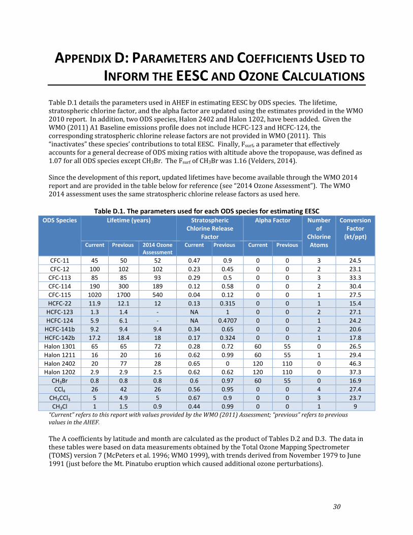
APPENDIX D: PARAMETERS AND COEFFICIENTS USED TOINFORM THE EESC AND OZONE CALCULATIONS

Table D.1 details the parameters used in AHEF in estimating EESC by ODS species. The lifetime, stratospheric chlorine factor, and the alpha factor are updated using the estimates provided in the WMO 2010 report. In addition, two ODS species, Halon 2402 and Halon 1202, have been added. Given the WMO (2011) A1 Baseline emissions profile does not include HCFC-123 and HCFC-124, the corresponding stratospheric chlorine release factors are not provided in WMO (2011). This “inactivates” these species’ contributions to total EESC. Finally, Fsurf, a parameter that effectively accounts for a general decrease of ODS mixing ratios with altitude above the tropopause, was defined as 1.07 for all ODS species except CH3Br. The Fsurf of CH3Br was 1.16 (Velders, 2014).

Since the development of this report, updated lifetimes have become available through the WMO 2014 report and are provided in the table below for reference (see “2014 Ozone Assessment”). The WMO 2014 assessment uses the same stratospheric chlorine release factors as used here.

Table D.1. The parameters used for each ODS species for estimating EESC ODS Species Lifetime (years) Stratospheric

Chlorine Release Factor

Alpha Factor Number of

Chlorine Atoms

Conversion Factor

(kt/ppt) Current Previous 2014 Ozone

Assessment Current Previous Current Previous

CFC-11 45 50 52 0.47 0.9 0 0 3 24.5 CFC-12 100 102 102 0.23 0.45 0 0 2 23.1

CFC-113 85 85 93 0.29 0.5 0 0 3 33.3 CFC-114 190 300 189 0.12 0.58 0 0 2 30.4 CFC-115 1020 1700 540 0.04 0.12 0 0 1 27.5 HCFC-22 11.9 12.1 12 0.13 0.315 0 0 1 15.4

HCFC-123 1.3 1.4 - NA 1 0 0 2 27.1 HCFC-124 5.9 6.1 - NA 0.4707 0 0 1 24.2

HCFC-141b 9.2 9.4 9.4 0.34 0.65 0 0 2 20.6 HCFC-142b 17.2 18.4 18 0.17 0.324 0 0 1 17.8 Halon 1301 65 65 72 0.28 0.72 60 55 0 26.5 Halon 1211 16 20 16 0.62 0.99 60 55 1 29.4 Halon 2402 20 77 28 0.65 0 120 110 0 46.3 Halon 1202 2.9 2.9 2.5 0.62 0.62 120 110 0 37.3

CH3Br 0.8 0.8 0.8 0.6 0.97 60 55 0 16.9 CCl4 26 42 26 0.56 0.95 0 0 4 27.4

CH3CCl3 5 4.9 5 0.67 0.9 0 0 3 23.7 CH3Cl 1 1.5 0.9 0.44 0.99 0 0 1 9

“Current” refers to this report with values provided by the WMO (2011) Assessment; “previous” refers to previous values in the AHEF.

The A coefficients by latitude and month are calculated as the product of Tables D.2 and D.3. The data in these tables were based on data measurements obtained by the Total Ozone Mapping Spectrometer (TOMS) version 7 (McPeters et al. 1996; WMO 1999), with trends derived from November 1979 to June 1991 (just before the Mt. Pinatubo eruption which caused additional ozone perturbations).

30

Table D.2. Ozone Vertical Column (Dobson units) for 1980 by latitude band and month Latitude

Band (oN)

Month Jan Feb Mar Apr May Jun Jul Aug Sep Oct Nov Dec

20 to 30 261 264 274 288 299 296 293 283 283 275 266 266 30 to 40 311 324 335 334 336 321 307 301 291 283 283 302 40 to 50 364 398 398 392 378 356 333 319 307 313 313 336 50 to 60 388 418 440 426 404 375 352 330 321 330 330 345 60 to 70 0 408 455 448 413 371 342 319 311 0 0 0

Table D.3. Ozone trend (% per decade) from 1980 to 1990 by latitude band and month Latitude

Band (oN)

Month Jan Feb Mar Apr May Jun Jul Aug Sep Oct Nov Dec

20 to 30 -2.1 -1.8 -1.0 -0.5 -0.5 -1.0 -1.4 -1.3 -0.9 -0.7 -1.1 -1.7 30 to 40 -4.2 -5.1 -4.4 -2.8 -1.6 -1.5 -2.2 -2.4 -1.7 -0.6 -0.7 -2.3 40 to 50 -3.7 -5.4 -5.8 -4.7 -3.0 -2.0 -2.0 -2.5 -2.2 -1.1 -0.5 -1.5 50 to 60 -0.7 -2.6 -4.3 -4.8 -4.1 -2.9 -2.4 -2.9 -3.3 -2.5 -0.8 0.2 60 to 70 0.0 0.0 -3.2 -4.6 -4.5 -3.5 -2.7 -3.0 -3.6 -2.7 0.0 0.0

31

APPENDIX E: TOTAL COLUMN OZONE FOR MODELEDPOLICY SCENARIOS

Figure E-1 presents total column ozone associated with three policy scenarios: no policy controls; the 1987 Montreal Protocol; and the Montreal Protocol as amended and adjusted through the 2007 Montreal Adjustment. Total column ozone is shown for two versions of the AHEF—the previous VM-based AHEF as used prior to the updates made through this report; and the updated WMO-based AHEF that incorporates the modeling changes described in this report. As shown, the total column ozone modeled for the 1987 Montreal Protocol and 2007 Montreal Adjustment are relatively similar between the VM-based and WMO-based versions of the AHEF; however, the no controls scenario is significantly different, which has implications for estimating human health benefits relative to no policy controls.

Figure E-1: Total Column Ozone Associated with No Controls, 1987 Montreal Protocol, and 2007 Montreal Adjustment Policy Scenarios

32

APPENDIX F: EXPLANATION OF DIFFERENCES BETWEENVM1999 AND VM2012

This table provides a description of the major VM updates that affect the emission estimates of each species between VM1999 and VM2012. Future U.S. based policy scenarios would be developed using the latest VM.

Table F.1: Explanation of Differences between VM1999 and VM2012 Species Differences Explanation for Differences

CFC-11 Emissions continue through 2050 in VM4.4 (emissions end in 2039 in VM 1999), and are lower in VM4,4

Many Ref transitions away from CFC-11 began earlier than 1996

CFC-12 Overall, lower emissions in VM4.4 Many Ref transitions away from CFC-12 began earlier than 1996

HCFC-22 Higher emissions in VM4.4 Reflection of major uses of HCFC-22 as a CFC alternative (most commonly used HCFC; used in Ref, AC, and foam applications)

CFC-113 Latest VM phases out CFC-113 by 1996, otherwise, relatively similar

Emissions consistent with Montreal Protocol phaseout schedule

CT (CCl4) VM4.4 has much lower emissions, which end in 1996

Emissions consistent with Montreal Protocol phaseout schedule and niche solvent applications of CT

MCF Similar emissions until 1996, VM4.4 emissions end

Emissions consistent with Montreal Protocol phaseout schedule and niche solvent applications of MCF

CH3Cl None NA

Halon 1301 Lower emissions in VM4.4 through 2032, Higher emissions in VM4.4 through 2050

Critical uses of Halon 1301 for fire suppression

Halon 1211 Lower emissions in VM4.4 through 2029, Higher emissions in VM4.4 through 2050

Critical uses of Halon 1211 for fire suppression

CH3Br Not included in either version of VM NA

HCFC-123 Lower emissions in VM4.4 through 2020, then higher emissions through 2050

Used as a flooding agent (through 2014) and chillers (no phaseout)

HCFC-124 Lower emissions in VM4.4 Relatively small uses in Ref, sterilization, and FireExt

HFC-125 Introduced sooner in VM4.4; similar emissions through 2030 then fewer emissions than VM 1999 through 2050

Used as an alternative in flooding agents, chillers, IPR, and other refrigeration equipment, but not the most common ODS replacement for those end uses

HFC-134a Higher emissions in VM4.4, not phased out in latest VM

Reflection of the high uses of HFC-134a (most commonly used HFC; used in Ref, AC, aerosols, and foam applications)

HCFC-141b

Historically similar emissions; VM4.4 emissions higher between 2010 and 2040, then lower than VM 1999 from 2041–2050

HCFC-141b used in foams with long lifetimes (between 14 and 56 years)

33

Table F.1: Explanation of Differences between VM1999 and VM2012 cont. Species Differences Explanation for Differences

HCFC-142b Introduced sooner in VM4.4 and with higher emissions continuing through 2050

Used in as a Ref blend and in foam; Emissions due to leakage and disposal

HFC-143 Not included in VM 1999 NA HFC-152 Higher emissions in VM4.4 HFC use has grown significantly

CFC-114 Relatively close CFC-114 used in chillers, foams, and aerosols. Not completely phased out of MDI aerosol use until 2014

CFC-115 Higher emissions in VM4.4 Refrigerant blend in large equipment (transport, large retail food, cold storage) with 20+ year lifetimes

34