Epifanio BMC Bioinformatics (2017) 18:230 DOI 10.1186/s12859-017-1650-8

METHODOLOGY ARTICLE Open Access

Intervention in prediction measure: a newapproach to assessing variable importance forrandom forestsIrene Epifanio

Abstract

Background: Random forests are a popular method in many fields since they can be successfully applied tocomplex data, with a small sample size, complex interactions and correlations, mixed type predictors, etc.Furthermore, they provide variable importance measures that aid qualitative interpretation and also the selection ofrelevant predictors. However, most of these measures rely on the choice of a performance measure. But measures ofprediction performance are not unique or there is not even a clear definition, as in the case of multivariate responserandom forests.Methods: A new alternative importance measure, called Intervention in Prediction Measure, is investigated. Itdepends on the structure of the trees, without depending on performance measures. It is compared with otherwell-known variable importance measures in different contexts, such as a classification problem with variables ofdifferent types, another classification problem with correlated predictor variables, and problems with multivariateresponses and predictors of different types.Results: Several simulation studies are carried out, showing the new measure to be very competitive. In addition, it isapplied in two well-known bioinformatics applications previously used in other papers. Improvements inperformance are also provided for these applications by the use of this new measure.Conclusions: This new measure is expressed as a percentage, which makes it attractive in terms of interpretability. Itcan be used with new observations. It can be defined globally, for each class (in a classification problem) andcase-wise. It can easily be computed for any kind of response, including multivariate responses. Furthermore, it can beused with any algorithm employed to grow each individual tree. It can be used in place of (or in addition to) othervariable importance measures.

Keywords: Random forest, Variable importance measure, Multivariate response, Feature selection, Conditionalinference trees

BackgroundHigh-dimensional problems, those that involve so-calledp > n data [1], are of great importance in many areas ofcomputational biology. Predicting problems in which thenumber of features or variables p is much larger than thenumber of samples or observations n is a statistical chal-lenge. In addition, many bioinformatics data sets containhighly correlated variables with complex interactions, andthey may also contain variables that are irrelevant to theprediction. Furthermore, data sets may contain data of a

Correspondence: epifanio@uji.esDepartament de Matemàtiques and Institut de Matemàtiques i Aplicacions deCastelló, Universitat Jaume I, Campus del Riu Sec, 12071 Castelló, Spain

mixed type, i.e. categorical (with a different number of cat-egories) and numerical, not only as predictors but also asoutputs or responses.Decision trees are a nonparametric and highly nonlin-

ear method that can be used successfully with that kind ofchallenging data. Furthermore, they are robust to outliersin the input space, invariant to monotone transforma-tions of numerical predictors, and can also handle missingvalues. Thanks to these properties, decision trees havebecome a very popular tool in bioinformatics and datamining problems in general.However, the predictive power of decision trees is their

Achilles heel. A bagging strategy can be considered to

© The Author(s). 2017 Open Access This article is distributed under the terms of the Creative Commons Attribution 4.0International License (http://creativecommons.org/licenses/by/4.0/), which permits unrestricted use, distribution, andreproduction in any medium, provided you give appropriate credit to the original author(s) and the source, provide a link to theCreative Commons license, and indicate if changes were made. The Creative Commons Public Domain Dedication waiver(http://creativecommons.org/publicdomain/zero/1.0/) applies to the data made available in this article, unless otherwise stated.

Epifanio BMC Bioinformatics (2017) 18:230 Page 2 of 16

improve their individual performance. A random forest(RF) is an ensemble of a large collection of trees [2]. Thereare several types of RFs according to the type of response.If the response is categorical, we refer to RF classification.If the response is continuous, we refer to RF regression.If the responses are right censored survival data, we referto Random Survival Forests. Multivariate RFs refer to RFswith multiple responses [3]. RFs with only one responseare applied to many different problems in bioinformatics[4, 5]. However, the number of studies with multivariateRFs is much smaller [6].Besides good performance, another advantage of RFs is

that they require little tuning. Another property of RFsthat makes them attractive is that they return variableimportance measures (VIMs). These VIMs can be usedto rank variables and identify those which most influenceprediction. This favors interpretability. Predictors are notusually equally relevant. In fact, often only a few of themhave a substantial influence on the response, i.e. the restof them are irrelevant and could have been excluded fromthe analysis. It is often useful to learn the contribution orimportance of explanatory variables in the response [1].The most widely used VIMs for RFs, such as the Gini

VIM (GVIM), permutation VIM (PVIM) and conditionalpermutation VIM (CPVIM) [7], rely on the choice of aperformance measure. However, measures of predictionperformance are not unique [8]. Some examples for clas-sification are misclassification cost, Brier score, sensitivityand specificity measures (binary problems), etc., whilesome examples for regression problems are mean squarederror, mean absolute error, etc. In the case of unbalanceddata, i.e. data where response class sizes differ consider-ably, the area under the curve (AUC) is suggested by [9]instead of the common error rate. There is no clear appro-priate performance measure for survival data [10], less soin the case of multivariate response and even less so if theresponses are of different types.To solve this issue, an approach for selecting vari-

ables that depends on the structure of the trees, withoutdepending on performance measures, was proposed by[10]. They proposed an algorithm based on the minimaldepth (MD) statistic, i.e. based on the idea that variablesthat tend to split close to the root node should have moreimportance in prediction. By removing the dependence onperformance measures, the arrangement of the trees gainsstrength, as in the case of splitting rules.Recently, the author has proposed a new alternative

importance measure in RFs called Intervention in Predic-tion Measure (IPM) [11] in an industrial application. IPMis also based on the structure of the trees, like MD. There-fore, it is independent of any prediction performancemeasure. IPM only depends on the forest and tree param-eter settings. However, unlike MD, IPM is a case-basedmeasure. Note also that IPM is expressed as a percentage,

which makes it attractive in terms of interpretability. IPMcan be used with new observations that were not usedin the RF construction, without needing to know theresponse, unlike other VIMs. IPM can be defined glob-ally, for each class (in a classification problem) and locally.In addition, IPM can easily be computed for any kind ofresponse, including multivariate responses. IPM can beused with any algorithm employed to grow each individ-ual tree, from the Classification And Regression Trees(CART) algorithm developed by [12] to Conditional Infer-ence Trees (CIT) [13].The objective of this work is to compare the new IPM

with other well-known VIMs in different contexts, such asa classification problem with variables of different types,another classification problem with correlated predictorvariables, and problems with multivariate responses andpredictors of different types. Several simulation studieswere carried out to show the competitiveness of IPM. Fur-thermore, the objective is also to stress the advantagesof using IPM in bioinformatics. Consequently, the use ofIPM is also illustrated in two well-known bioinformaticsapplications previously employed in other papers [14–16].Although the majority of the data used here are not p > n,they could be relevant to this kind of scenarios, but this issomething to be explored in the future.

MethodsRandom forestAs mentioned previously, trees are a nonlinear regressionprocedure. Trees are grown by binary recursive partition-ing. The broad idea behind binary recursive partitioning isto iteratively choose one of the predictors and the binarysplit in this variable in order to ultimately fit a constantmodel in each cell of the resulting partition, which con-stitutes the prediction. Two known problems with suchmodels are overfitting and a selection bias towards predic-tors with many possible splits or missing values [15]. Tosolve these problems, [13] proposed a conditional infer-ence framework (CIT) for recursive partitioning, which isalso applicable to multivariate response variables, and itwill be used with IPM.As outlined above, trees are a low-bias but high-

variance technique, which makes them especially suitedfor bagging [1]. Growing an ensemble of trees signifi-cantly increases the accuracy. The term random forest wascoined by [2] for techniques where random vectors thatcontrol the growth of each tree in the ensemble are gen-erated. This randomness comes from randomly choosinga group ofmtry (mtry << p) predictors to split on at eachnode and bootstrapping a sample from the training set.The non-selected cases are called out-of-bag (OOB).Here, RFs based on CART (CART-RF) and CIT (CIT-

RF) are considered since the VIMs reviewed later arebased on these. Both are implemented in R [17]. Breiman’s

Epifanio BMC Bioinformatics (2017) 18:230 Page 3 of 16

RF algorithm [2] is implemented in the R packagerandomForest [18, 19] and also in the R package ran-domForestSRC [20–22], while CIT-RF can be found inthe R package party [23–25]. Multivariate RFs can becomputed by the R package randomForestSRC and the Rpackage party, but not by the R package randomForest. Inthe R package randomForestSRC, for multivariate regres-sion responses, a composite normalized mean-squarederror splitting rule is used; for multivariate classificationresponses, a composite normalized Gini index splittingrule is used; and when both regression and classificationresponses are detected, a multivariate normalized com-posite split rule of mean-squared error and Gini indexsplitting is invoked.Regardless of the specific RF implementation, VIMs can

be computed, which are a helpful tool for data interpretationand feature selection. VIMs can be used to obtain a rank-ing of the predictors according to their association withthe response. In the following section, themost used VIMsare briefly reviewed and our IPM proposal is introduced.

Random forest variable importance measures and variableselection proceduresThe most popular VIMs based on RF include GVIM,PVIM and CPVIM. GVIM and PVIM are derived fromCART-RF and can be computed with the R packagerandomForest [18, 19]. PVIM can also be derived fromCIT-RF and obtained with the R package party [23–25].CPVIM is based on CIT-RF, and can be calculated usingthe R package party. A very popular stepwise procedurefor variable selection using PVIM is the one proposedby [26] (varSelRF), which is available from the R pack-age varSelRF [27, 28]. The procedure for variable selectionbased on the tree-based concept termed MD proposed by[10] (varSelMD) is available from the R package random-ForestSRC [20–22]. The results of the chosen variables forvariable selection methods can be interesting, althoughthe objective of variable selection methods is not reallyreturning the importance of variables, but returning a setof variables that are subject to a certain objective, such aspreserving accuracy in [26]. The underlying rationale isthat the accuracy of prediction will not change if irrelevantpredictors are removed, while it drops if relevant ones areremoved. Table 1 gives an overview of the methods.

GVIMGVIM is based on the node impurity measure for nodesplitting. The node impurity is measured by the Gini indexfor classification and by the residual sum of squares forregression. The importance of a variable is defined as thetotal decrease in node impurities from splitting on thevariable, averaged over all trees. It is a global measurefor each variable; it is not defined locally or by class (forclassification problems). When there are different types

of variables, GVIM is strongly biased in favor of contin-uous variables and variables with many categories (thestatistical reasons for this are well explained by [15]).

PVIMThe importance of variable k is measured by averagingover all trees the decrease in accuracy between the pre-diction error for the OOB data of each tree and the sameafter permuting that predictor variable.The PVIM derived from CIT-RF is referred to as PVIM-

CIT-RF. Although CIT-RF can fit multivariate responses,PVIM cannot be computed (as previously discussed, thereis no clear appropriate performance measure for multi-variate responses).The PVIM derived from CART-RF is referred to as

PVIM-CART-RF, which is scaled (normalized by the stan-dard deviation of the difference) by default in the ran-domForest function from the R package randomForest[18, 19]. The problems of this scaled measure are exploredby [29]. According to [30], PVIM is often very consistentwith GVIM. PVIM can be computed for each class, and itcan also be computed casewise. The local or casewise vari-able importance is the increase in percent of times a case iis OOB andmisclassified when the variable k is permuted.This option is available from the R package randomForest[18, 19], but not from the R package party [23–25].

CPVIMAn alternative version of PVIM to correct bias for cor-related variables is CPVIM, which uses a conditionalpermutation scheme [25]. According to [31], CPVIMwould be more appropriate if the objective is to iden-tify a set of truly influential predictors without consid-ering the correlated effects. Otherwise, PVIM would bepreferable, as correlations are an inherent mutual prop-erty of predictors. In CPVIM, the variable importance ofa predictor is computed conditionally on the values ofother associated/correlated predictor variables, i.e. possi-ble confounders are taken into account, unlike PVIM. Theconcept of confounding is well illustrated with a simpleexample considered in [32] (see [32] for a more extensiveexplanation): a classification problem for assessing fetalhealth during pregnancy. Let Y be the response with twopossible values (Y = 0 if the diagnosis is incorrect andY = 1 otherwise). Let us consider the following predic-tors: X1, which assesses the quality of ultrasound devicesin the hospital, X2, which assesses whether the hospitalstaff are trained to use them and interpret the imagesand X3, which assesses the cleanliness of hospital floors.Note that X2 is related to Y and X3, which are linkedto the hospital’s quality standards. If X2 was not takeninto account in the analysis, a strong association betweenY and X3 would probably be found, i.e. X2 would actas a confounder. In the multiple regression model, if X2

Epifanio BMC Bioinformatics (2017) 18:230 Page 4 of 16

Table

1Summaryof

somecharacteristicsof

VIMs

Metho

dsGVIM

PVIM

(CART-RF)

PVIM

(CIT-RF)

CPV

IMvarSelRF

varSelMD

IPM

Mainreferences

[43]

[2]

[13,15]

[25]

[26]

[10,33]

[11]andthis

manuscript

Keycharacteristic

Nod

eim

purity

Accuracyafter

variablepe

rmutation

Accuracyafter

variablepe

rmutation

Alte

rnativeof

PVIM;Con

ditio

nal

perm

utation

Backwardelim

ination

Variableselection

basedon

MD

Variables

interven

ing

inpred

ictio

n

RF-based

CART-RF

CART-RF

CIT-RF

CIT-RF

CART-RF

CART-RF

CART-RFor

CIT-RF

Handlingof

respon

seUnivariate

Univariate

Univariate

Univariate

Categ

orical

All(m

ultivariate

includ

ed)

All(m

ultivariate

includ

ed)

MainRim

plem

entatio

nrand

omForest[18,19]

rand

omForest[18,19]

rand

omForestSRC

[20–22]

party[23–25]

party[23–25]

varSelRF

[27,28]

rand

omForestSRC

[20–22]

Add

ition

alfile2

Casew

iseim

portance

No

Yes

Not

defin

edNot

defin

edNo

No

Yes

Epifanio BMC Bioinformatics (2017) 18:230 Page 5 of 16

was included as predictor in the model, the questionableinfluence of X3 would disappear. This is the underlyingrationale for CPVIM: conditionally on X2, X3 does nothave any effect on Y .

varSelRFDíaz-Uriarte and Alvarez de Andrés [26] presented abackward elimination procedure using RF for selectinggenes from microarray data. This procedure only appliesto RF classification. They examine all forests that resultfrom iteratively eliminating a fraction (0.2 by default) ofthe least important predictors used in the previous iter-ation. They use the unscaled version of PVIM-CART-RF.After fitting all forests, they examine the OOB error ratesfrom all the fitted random forests. The OOB error rate isan unbiased estimate of the test set error [30]. They selectthe solution with the smallest number of genes whoseerror rate is within 1 (by default) standard error of theminimum error rate of all forests.

varSelMDMD assesses the predictiveness of a variable by its depthrelative to the root node of a tree. A smaller value corre-sponds to a more predictive variable [33]. Specifically, theMD of a predictor variable v is the shortest distance fromthe root of the tree to the root of the closest maximal sub-tree of v; and a maximal subtree for v is the largest subtreewhose root node is split using v, i.e. no other parent nodeof the subtree is split using v. MD can be computed for anykind of RF, including multivariate RF.A high-dimensional variable selection method based on

the MD concept was introduced by [10]. It uses all dataand all variables simultaneously. Variables with an averageMD for the forest that exceeds themeanMD threshold areclassified as noisy and are removed from the final model.

Intervention in prediction measure (IPM)IPM was proposed in [11], where an RF with tworesponses (an ordered factor and a numeric variable) wasused for child garment size matching.IPM is a case-wise technique, i.e. IPM can be computed

for each case, whether new or used in the training set.This is a different perspective for addressing the problemof importance variables.The IPM of a new case, i.e. one not used to grow the for-

est and whose true response does not need to be known,is computed as follows. The new case is put down each ofthe ntree trees in the forest. For each tree, the case goesfrom the root node to a leaf through a series of nodes. Thevariable split in these nodes is recorded. The percentageof times a variable is selected along the case’s way fromthe root to the terminal node is calculated for each tree.Note that we do not count the percentage of times a splitoccurred on variable k in tree t, but only the variables that

intervened in the prediction of the case. The IPM for thisnew case is obtained by averaging those percentages overthe ntree trees. Therefore, for IPM computation it is onlynecessary to know the structure of the trees forming theforest; the response is not necessary.The IPM for a case in the training set is calculated by

considering and averaging over only the trees where thecase belongs to the OOB set. Once the casewise IPMs areestimated, the IPM can be computed for each class (in thecase of RF-classification) and globally, averaging over thecases in each class or all the cases, respectively. Since itis a case-wise technique, it is also possible to estimate theIPM for subsets of data, with no need to regrow the forestfor those subsets.An anonymous reviewer raised the question of using in-

sample observations in the IPM estimation. In fact, thecomplete sample could be used, which would increase thesample size. This is a matter for future study. AlthoughIPM is not based on prediction, i.e. it does not need theresponses for its computation once the RF is built, theresponses of in-sample observations were effectively usedin the construction of the trees. So brand new and unuseddata (OOB observations) were preferred for IPM estima-tion, in order to ensure generalization. In Additional file 1,there is an example using all samples.The new IPM and all of the code to reproduce the results

are available in Additional file 2.

Comparison studiesThe performance of IPM in relation to the other well-established VIMs is compared in several scenarios, withsimulated and real data. Two different kinds of responsesare analyzed with both simulated and real data, specif-ically RF-classification and Multivariate RF are consid-ered in order to cover the broadest possible spectrum ofresponses.The importance of the variables is known a priori with

simulated data, as we know the model which generatedthe data. In this way, we can reliably analyze the successesin the ranking and variable selection for each method,and also the stability of the results, as different data setsare generated for each model. For RF-classification, thesimulation models are analogous to those considered inprevious works. For Multivariate RFs, simulation modelsare designed starting from scratch in order to analyze theirperformance under different situations.Analyses are also conducted on real data, which have

previously been analyzed in the literature in order to sup-ply additional evidence based on realistic bioinformaticsdata structures that usually incorporate complex interde-pendencies.Once importance values are computed, predictors can

be ranked in decreasing order of importance, i.e. themost important variable appears in first place. For some

Epifanio BMC Bioinformatics (2017) 18:230 Page 6 of 16

methods there are ties (two variables are equally impor-tant). In such cases, the average ranking is used for thosevariables.All the computations are made in R [17]. The packages

and parameters used are detailed for each study.

Simulated dataCategorical response: Scenarios 1 and 2Two classification problems are simulated. In both cases,a binary response Y has to be predicted from a set ofpredictors.In the first scenario, the simulation design was similar to

that used in [15], where predictors varied in their scale andnumber of categories. The first predictor X1 was contin-uous, the other predictors from X2 to X5 were categoricalwith a different number of categories. Only predictor X2intervened in the generation of the response Y , i.e. onlyX2 was important, the other variables were uninforma-tive, i.e. noise. This should be reflected in the VIM results.The simulation design of Scenario 1 appears in Table 2.The number of cases (predictors and response) gener-ated in each data set was 120. A total of 100 data setswere generated, so the stability of the results could also beassessed.The parameter settings for RFs were as follows. CART-

RF was computed with bootstrap sampling withoutreplacement, with ntree = 50 as in [15], and two valuesfor mtry: 2 (sqrt(p) the default value in [18]) and 5 (equalto p). GVIM, PVIM and IPM were computed for CART-RF. CIT-RF was computed with the settings suggested forthe construction of an unbiased RF in [15], again withntree = 50 andmtry equal to 2 and 5. PVIM, CPVIM, andIPM were computed for CIT-RF. varSelRF [27] was usedwith the default parameters (ntree = 5000). varSelMD[20] was used with the default parameters (ntree = 1000andmtry = 2) and also withmtry = 5.The simulation design for the second scenario was

inspired by the set-up in [25, 31, 34]. The binary responseY was modeled by means of a logistic model:

P(Y = 1|X = x) = exTβ

1 + exTβ

where the coefficients β were: β = (5, 5, 2, 0,−5,−5,−2,0, 0, 0, 0, 0)T . The twelve predictors followed a multivari-ate normal distribution with mean vector μ = 0 andcovariance matrix �, with σj,j = 1 (all variables had unit

variance), σj,j′ = 0.9 for j �= j′ ≤ 4 (the first four vari-ables were block-correlated) and the other variables wereindependent with σj,j′ = 0. The behavior of VIMs underpredictor correlation could be studied with this model. Asbefore, 120 observations were generated for 100 data sets.The parameter settings for RFs were as follows. CART-

RF was computed with bootstrap sampling withoutreplacement, with ntree = 500 as in [25], and two valuesformtry: 3 (sqrt(p) the default value in [18]) and 12 (equalto p). GVIM, PVIM and IPM were computed for CART-RF. CIT-RF was computed with the settings suggested forthe construction of an unbiased RF in [15], again withntree = 500 and mtry equal to 3 and 12. PVIM, CPVIM,and IPM were computed for CIT. varSelRF was used withthe default parameters (ntree= 5000). varSelMDwas usedwith the default parameters (ntree = 1000 and mtry = 3)and also withmtry = 12.

Multivariate responses: Scenarios 3 and 4Again two scenarios were simulated. The design of thesimulated data was inspired by the type of variable com-position of the real problem with multivariate responsesthat would be analyzed. In this problem, responses werecontinuous and there were continuous and categoricalpredictors.The configuration of the third and fourth scenarios were

quite similar. Table 3 reports the predictor distributions,which were identical in both scenarios. Table 4 reportsthe response distributions, two continuous responses perscenario. Of the 7 predictors, only two were involved inthe response simulation: the binary X1 and the continuousX2. However, in the fourth scenario X2 only participatedin the response generation when X1 = 0. This arrange-ment was laid out in this way to analyze the ability of themethods to detect this situation. The rest of the predictorsdid not take part in the response generation, but X5 wasvery highly correlated with X2. In addition, the noise pre-dictors X6 (continuous) and X7 (categorical) were createdby randomly permuting the values of X2 and X1, respec-tively, as in [10]. The other irrelevant predictors,X3 andX4were continuous with different distributions. As before,120 observations in each scenario were generated for 100data sets.With multivariate responses, only two VIMs could be

computed. varSelMD was used with the default parame-ters (ntree = 1000 and mtry = 3) and also with mtry = 7.IPMwas computed for CIT-RFwith the settings suggested

Table 2 Simulation design for Scenario 1

Variables X1 X2 X3 X4 X5 Y|X2 = 0 Y|X2 = 1

Distribution N(0,1) B(1,0.5) DU(1/4) DU(1/10) DU(1/20) B(1,0.5 - rel) B(1,0.5 + rel)

The variables are sampled independently from the following distributions. N(0,1) stands for the standard normal distribution. B(1,π ) stands for the Binomial distribution withn = 1, i.e the Bernoulli distribution, and probability π . DU(1/n) stands for the Discrete Uniform distribution with values 1, . . . , n. The relevance parameter rel indicates thedegree of dependence between Y and X2, and is set at 0.1, which is not very high

Epifanio BMC Bioinformatics (2017) 18:230 Page 7 of 16

Table 3 Simulation design of predictors for Scenario 3 and 4

Variables X1 X2 X3 X4 X5 X6 X7

Distribution B(1,0.6) N(3,1) Unif(4,6) N(5,1) X2 + N(0,0.15) P(X2) P(X1)

The variables are sampled independently from the following distributions. B(1,π ) stands for the Binomial distribution with n = 1, i.e the Bernoulli distribution, and probabilityπ . N(μ, σ ) stands for the normal distribution with mean μ and standard deviation σ . Unif(a, b) stands for the continuous uniform distribution on the interval [ a, b]. P(X) standsfor random permutation of the values generated in the variable X

for the construction of an unbiased RF in [15], withntree = 1000 andmtry = 7.

Real data: Application to C-to-U conversion data andapplication to nutrigenomic studyTwo well-known real data sets were analyzed. The firstwas a binary classification problem, where the predic-tors were of different types. In the second, the responsewas multivariate and the predictors were continuous andcategorical, as in the first set.The first data set was the Arabidopsis thaliana, Brassica

napus, and Oryza sativa data from [14, 15], which can bedownloaded from Additional file 2. It applies to C-to-Uconversion data. RNA editing is the process whereby RNAis modified from the sequence of the corresponding DNAtemplate [14, 15]. For example, cytidine-to-uridine (C-to-U) conversion is usual in plant mitochondria. Althoughthe mechanisms of this conversion are not known, itseems that the neighboring nucleotides are important.Therefore, the data set is formed by 876 cases, each ofthem with the following recorded variables (one responseand 43 predictors):

• Edit, with two values (edited or not edited at the siteof interest). This is the binary response variable.

• The 40 nucleotides at positions –20 to 20 (namedwith those numbers), relative to the edited site, with 4categories;

• the codon position, cp, which is categorical with 4categories;

• the estimated folding energy, fe, which is continuous,and

• the difference in estimated folding energy (dfe)between pre-edited and edited sequences, which iscontinuous.

The second data set derives from a nutrigenomic study[16] and is available in the R package randomForestSRC[20] and Additional file 2. The study examines the effectsof 5 dietary treatments on 21 liver lipids and 120 hepatic

gene expressions in wild-type and PPAR-alpha deficientmice. Therefore, the continuous responses are the lipidexpressions (21 variables), while the predictors are thecontinuous gene expressions (120 variables), the diet (cat-egorical with 5 categories), and the genotype (categoricalwith 2 categories). The number of observations is 40.According to [16], in vivo studies were conducted underEuropean Union guidelines for the use and care of lab-oratory animals and were approved by their institutionalethics committee.

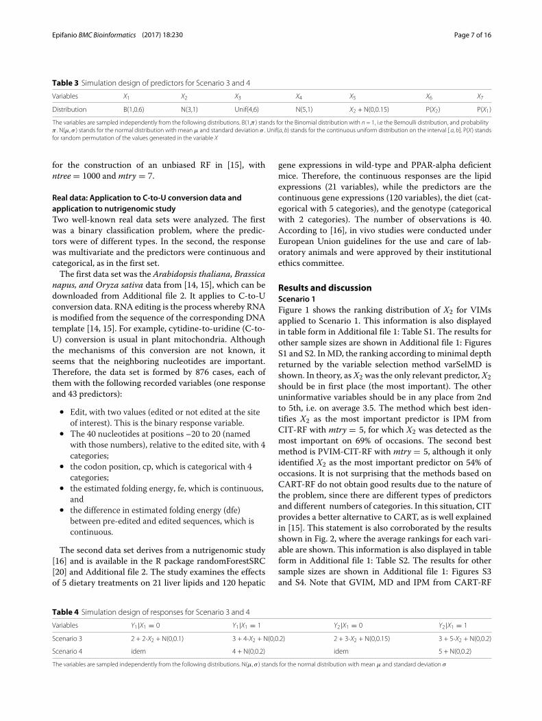
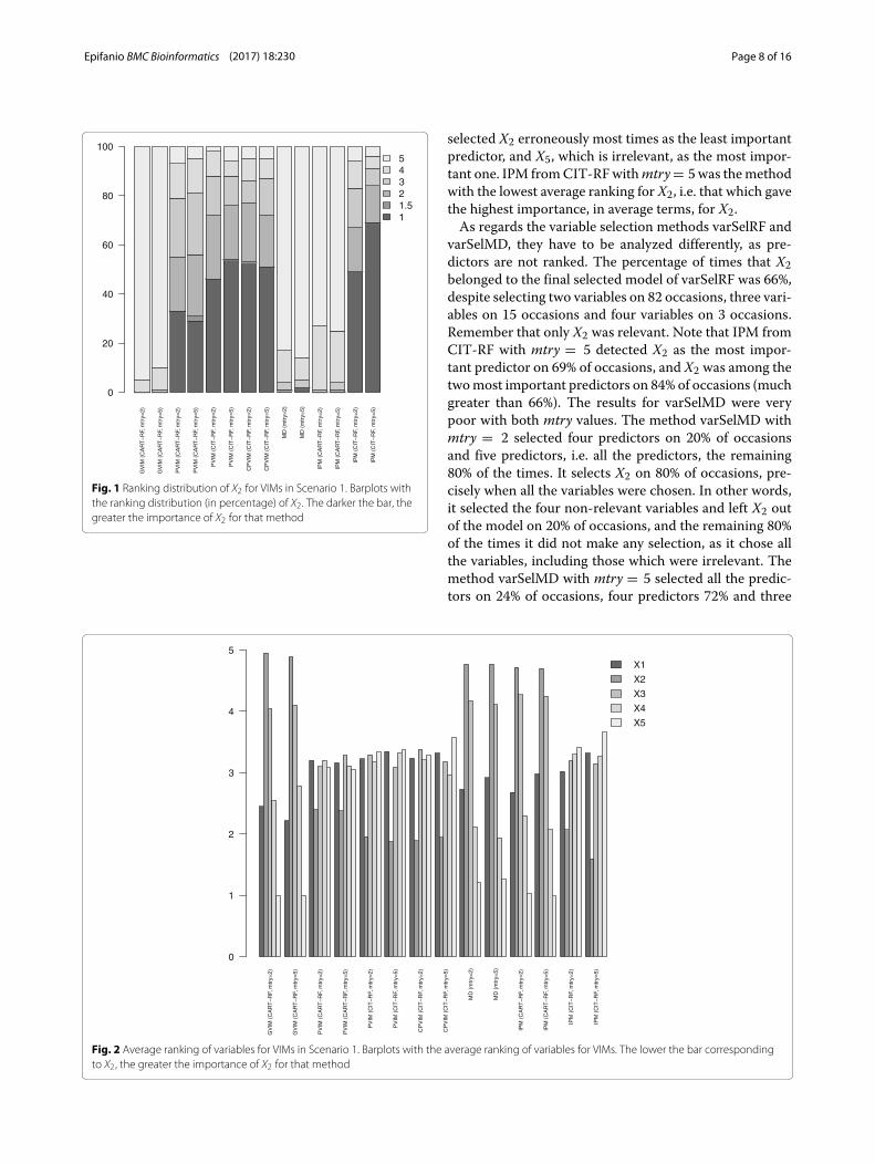
Results and discussionScenario 1Figure 1 shows the ranking distribution of X2 for VIMsapplied to Scenario 1. This information is also displayedin table form in Additional file 1: Table S1. The results forother sample sizes are shown in Additional file 1: FiguresS1 and S2. InMD, the ranking according to minimal depthreturned by the variable selection method varSelMD isshown. In theory, as X2 was the only relevant predictor, X2should be in first place (the most important). The otheruninformative variables should be in any place from 2ndto 5th, i.e. on average 3.5. The method which best iden-tifies X2 as the most important predictor is IPM fromCIT-RF with mtry = 5, for which X2 was detected as themost important on 69% of occasions. The second bestmethod is PVIM-CIT-RF with mtry = 5, although it onlyidentified X2 as the most important predictor on 54% ofoccasions. It is not surprising that the methods based onCART-RF do not obtain good results due to the nature ofthe problem, since there are different types of predictorsand different numbers of categories. In this situation, CITprovides a better alternative to CART, as is well explainedin [15]. This statement is also corroborated by the resultsshown in Fig. 2, where the average rankings for each vari-able are shown. This information is also displayed in tableform in Additional file 1: Table S2. The results for othersample sizes are shown in Additional file 1: Figures S3and S4. Note that GVIM, MD and IPM from CART-RF

Table 4 Simulation design of responses for Scenario 3 and 4

Variables Y1|X1 = 0 Y1|X1 = 1 Y2|X1 = 0 Y2|X1 = 1

Scenario 3 2 + 2·X2 + N(0,0.1) 3 + 4·X2 + N(0,0.2) 2 + 3·X2 + N(0,0.15) 3 + 5·X2 + N(0,0.2)

Scenario 4 idem 4 + N(0,0.2) idem 5 + N(0,0.2)

The variables are sampled independently from the following distributions. N(μ, σ ) stands for the normal distribution with mean μ and standard deviation σ

Epifanio BMC Bioinformatics (2017) 18:230 Page 8 of 16

GV

IM (

CA

RT

−R

F, m

try=

2)

GV

IM (

CA

RT

−R

F, m

try=

5)

PV

IM (

CA

RT

−R

F, m

try=

2)

PV

IM (

CA

RT

−R

F, m

try=

5)

PV

IM (

CIT

−R

F, m

try=

2)

PV

IM (

CIT

−R

F, m

try=

5)

CP

VIM

(C

IT−

RF,

mtr

y=2)

CP

VIM

(C

IT−

RF,

mtr

y=5)

MD

(m

try=

2)

MD

(m

try=

5)

IPM

(C

AR

T−

RF,

mtr

y=2)

IPM

(C

AR

T−

RF,

mtr

y=5)

IPM

(C

IT−

RF,

mtr

y=2)

IPM

(C

IT−

RF,

mtr

y=5)

54321.51

0

20

40

60

80

100

Fig. 1 Ranking distribution of X2 for VIMs in Scenario 1. Barplots withthe ranking distribution (in percentage) of X2. The darker the bar, thegreater the importance of X2 for that method

selected X2 erroneously most times as the least importantpredictor, and X5, which is irrelevant, as the most impor-tant one. IPM fromCIT-RFwithmtry= 5 was themethodwith the lowest average ranking for X2, i.e. that which gavethe highest importance, in average terms, for X2.As regards the variable selection methods varSelRF and

varSelMD, they have to be analyzed differently, as pre-dictors are not ranked. The percentage of times that X2belonged to the final selected model of varSelRF was 66%,despite selecting two variables on 82 occasions, three vari-ables on 15 occasions and four variables on 3 occasions.Remember that only X2 was relevant. Note that IPM fromCIT-RF with mtry = 5 detected X2 as the most impor-tant predictor on 69% of occasions, and X2 was among thetwomost important predictors on 84% of occasions (muchgreater than 66%). The results for varSelMD were verypoor with both mtry values. The method varSelMD withmtry = 2 selected four predictors on 20% of occasionsand five predictors, i.e. all the predictors, the remaining80% of the times. It selects X2 on 80% of occasions, pre-cisely when all the variables were chosen. In other words,it selected the four non-relevant variables and left X2 outof the model on 20% of occasions, and the remaining 80%of the times it did not make any selection, as it chose allthe variables, including those which were irrelevant. Themethod varSelMD with mtry = 5 selected all the predic-tors on 24% of occasions, four predictors 72% and three

GV

IM (

CA

RT

−R

F, m

try=

2)

GV

IM (

CA

RT

−R

F, m

try=

5)

PV

IM (

CA

RT

−R

F, m

try=

2)

PV

IM (

CA

RT

−R

F, m

try=

5)

PV

IM (

CIT

−R

F, m

try=

2)

PV

IM (

CIT

−R

F, m

try=

5)

CP

VIM

(C

IT−

RF,

mtr

y=2)

CP

VIM

(C

IT−

RF,

mtr

y=5)

MD

(m

try=

2)

MD

(m

try=

5)

IPM

(C

AR

T−

RF,

mtr

y=2)

IPM

(C

AR

T−

RF,

mtr

y=5)

IPM

(C

IT−

RF,

mtr

y=2)

IPM

(C

IT−

RF,

mtr

y=5)

X1

X2

X3

X4

X5

0

1

2

3

4

5

Fig. 2 Average ranking of variables for VIMs in Scenario 1. Barplots with the average ranking of variables for VIMs. The lower the bar correspondingto X2, the greater the importance of X2 for that method

Epifanio BMC Bioinformatics (2017) 18:230 Page 9 of 16

predictors 4%. X2 was among those selected on only 26%of occasions (when all the variable were selected on 24%of occasions).IPM values are also easy to interpret, since they are pos-

itive and add one. The average IPM (from CIT-RF withmtry = 5) values of cases in the 100 data sets for eachvariable were: 0.18 (X1), 0.31 (X2), 0.18 (X3), 0.17 (X4) and0.16 (X5). So X2 was the most important, whereas it gavemore or less the same importance to the other variables.An issue for further research is to determine from whichthreshold (maybe depending on the number of variables)a predictor can be considered irrelevant.IPM can also be computed in class-specific terms, as

PVIM-CART-RF. (They can also be computed casewise,but we omit those results in the interests of brevity). As anillustrative example, results from a data set are examined.In [11] we showed two problems for which the resultsof IPM by class were more consistent with that expectedthan those of PVIM-CART-RF by class, and this is also thecase with the current problem. Table 5 shows the impor-tance measures by group and globally. The IPM rankingsseem to be more consistent at a glance than those forPVIM-CART-RF. For instance, the ranking by PVIM forclass 1 gave X1 as the most important predictor, whereasX1 was the fourth (the penultimate) most important pre-dictor for class 0. We computed Kendall’s coefficient W[35] to assess the concordance. Kendall’s coefficient Wis an index of inter-rater reliability of ordinal data [36].Kendall’s W ranges from 0 (no agreement) to 1 (com-plete agreement). Kendall’s W for the ranking of PVIMCART-RF (mtry = 2) for class 0 and 1 was 0.5, whereasfor IPM CIT-RF (mtry = 5) it was 0.95. We repeated thisprocedure for each of the 100 data sets, and the aver-age Kendall’s W were 0.71 and 0.96 for PVIM-CART-RF(mtry = 2) and IPM CIT-RF (mtry = 5), respectively.Therefore, the agreement between the class rankings forIPM was very high. Note that in this case, the impor-tance of predictors followed the same pattern for eachresponse class as reflected by the IPM results, but it could

Table 5 Analysis by class of a data set in Scenario 1

Measures PVIM IPM

0 1 G 0 1 G

X1 4 1 4 3 3 3

X2 2 3 2 1 1 1

X3 3 2 3 5 4 5

X4 1 4 1 2 2 2

X5 5 5 5 4 5 4

The first column is the name of the variables. The two following columnscorrespond to the PVIM ranking (CART-RF,mtry = 2) for each class, whereas the thirdcolumn is the same but calculated globally (labeled as G). The last three columnscontain the ranking of the IPM values (CIT-RF,mtry = 5) first by group and the lastcolumn computed globally (labeled as G)

be different in other cases. This has great potential inapplied research, as explained in [32, 37]: for example, dif-ferent predictors may be informative with different cancersubtypes.

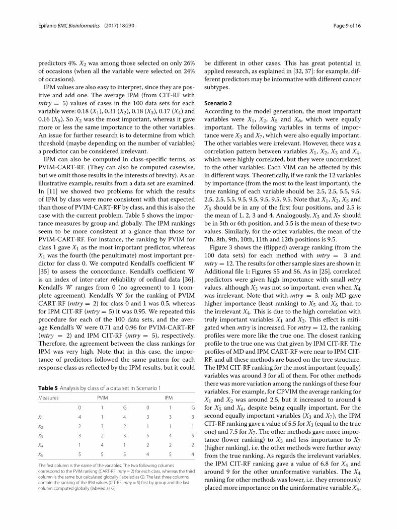
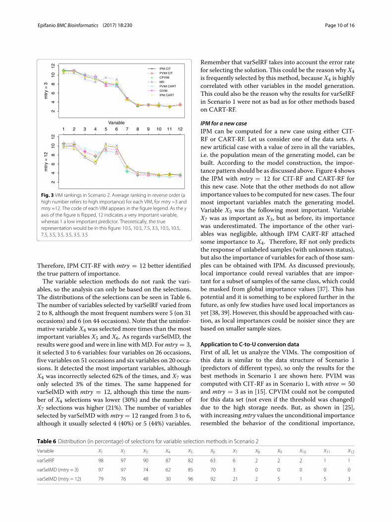
Scenario 2According to the model generation, the most importantvariables were X1, X2, X5 and X6, which were equallyimportant. The following variables in terms of impor-tance were X3 and X7, which were also equally important.The other variables were irrelevant. However, there was acorrelation pattern between variables X1, X2, X3 and X4,which were highly correlated, but they were uncorrelatedto the other variables. Each VIM can be affected by thisin different ways. Theoretically, if we rank the 12 variablesby importance (from the most to the least important), thetrue ranking of each variable should be: 2.5, 2.5, 5.5, 9.5,2.5, 2.5, 5.5, 9.5, 9.5, 9.5, 9.5, 9.5. Note that X1, X2, X5 andX6 should be in any of the first four positions, and 2.5 isthe mean of 1, 2, 3 and 4. Analogously, X3 and X7 shouldbe in 5th or 6th position, and 5.5 is the mean of these twovalues. Similarly, for the other variables, the mean of the7th, 8th, 9th, 10th, 11th and 12th positions is 9.5.Figure 3 shows the (flipped) average ranking (from the

100 data sets) for each method with mtry = 3 andmtry = 12. The results for other sample sizes are shown inAdditional file 1: Figures S5 and S6. As in [25], correlatedpredictors were given high importance with small mtryvalues, although X3 was not so important, even when X4was irrelevant. Note that with mtry = 3, only MD gavehigher importance (least ranking) to X5 and X6 than tothe irrelevant X4. This is due to the high correlation withtruly important variables X1 and X2. This effect is miti-gated when mtry is increased. For mtry = 12, the rankingprofiles were more like the true one. The closest rankingprofile to the true one was that given by IPM CIT-RF. Theprofiles of MD and IPM CART-RF were near to IPM CIT-RF, and all these methods are based on the tree structure.The IPMCIT-RF ranking for the most important (equally)variables was around 3 for all of them. For other methodsthere was more variation among the rankings of these fourvariables. For example, for CPVIM the average ranking forX1 and X2 was around 2.5, but it increased to around 4for X5 and X6, despite being equally important. For thesecond equally important variables (X3 and X7), the IPMCIT-RF ranking gave a value of 5.5 forX3 (equal to the trueone) and 7.5 for X7. The other methods gave more impor-tance (lower ranking) to X3 and less importance to X7(higher ranking), i.e. the other methods were further awayfrom the true ranking. As regards the irrelevant variables,the IPM CIT-RF ranking gave a value of 6.8 for X4 andaround 9 for the other uninformative variables. The X4ranking for other methods was lower, i.e. they erroneouslyplacedmore importance on the uninformative variableX4.

Epifanio BMC Bioinformatics (2017) 18:230 Page 10 of 16

24

68

1012

mtr

y =

3

IPM CIT

PVIM CIT

CPVIM

MD

PVIM CART

GVIM

IPM CART

Variable

24

68

1012

mtr

y =

12

1 2 3 4 5 6 7 8 9 10 11 12

Fig. 3 VIM rankings in Scenario 2. Average ranking in reverse order (ahigh number refers to high importance) for each VIM, formtry =3 andmtry =12. The code of each VIM appears in the figure legend. As the yaxis of the figure is flipped, 12 indicates a very important variable,whereas 1 a low important predictor. Theoretically, the truerepresentation would be in this figure: 10.5, 10.5, 7.5, 3.5, 10.5, 10.5,7.5, 3.5, 3.5, 3.5, 3.5, 3.5

Therefore, IPM CIT-RF with mtry = 12 better identifiedthe true pattern of importance.The variable selection methods do not rank the vari-

ables, so the analysis can only be based on the selections.The distributions of the selections can be seen in Table 6.The number of variables selected by varSelRF varied from2 to 8, although the most frequent numbers were 5 (on 31occasions) and 6 (on 44 occasions). Note that the uninfor-mative variable X4 was selected more times than the mostimportant variables X5 and X6. As regards varSelMD, theresults were good and were in line withMD. Formtry = 3,it selected 3 to 6 variables: four variables on 26 occasions,five variables on 51 occasions and six variables on 20 occa-sions. It detected the most important variables, althoughX4 was incorrectly selected 62% of the times, and X7 wasonly selected 3% of the times. The same happened forvarSelMD with mtry = 12, although this time the num-ber of X4 selections was lower (30%) and the number ofX7 selections was higher (21%). The number of variablesselected by varSelMD withmtry = 12 ranged from 3 to 6,although it usually selected 4 (40%) or 5 (44%) variables.

Remember that varSelRF takes into account the error ratefor selecting the solution. This could be the reason why X4is frequently selected by this method, because X4 is highlycorrelated with other variables in the model generation.This could also be the reason why the results for varSelRFin Scenario 1 were not as bad as for other methods basedon CART-RF.

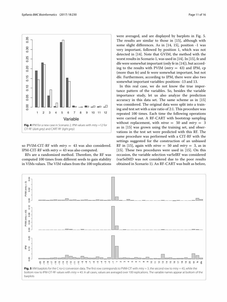
IPM for a new caseIPM can be computed for a new case using either CIT-RF or CART-RF. Let us consider one of the data sets. Anew artificial case with a value of zero in all the variables,i.e. the population mean of the generating model, can bebuilt. According to the model construction, the impor-tance pattern should be as discussed above. Figure 4 showsthe IPM with mtry = 12 for CIT-RF and CART-RF forthis new case. Note that the other methods do not allowimportance values to be computed for new cases. The fourmost important variables match the generating model.Variable X3 was the following most important. VariableX7 was as important as X3, but as before, its importancewas underestimated. The importance of the other vari-ables was negligible, although IPM CART-RF attachedsome importance to X4. Therefore, RF not only predictsthe response of unlabeled samples (with unknown status),but also the importance of variables for each of those sam-ples can be obtained with IPM. As discussed previously,local importance could reveal variables that are impor-tant for a subset of samples of the same class, which couldbe masked from global importance values [37]. This haspotential and it is something to be explored further in thefuture, as only few studies have used local importances asyet [38, 39]. However, this should be approached with cau-tion, as local importances could be noisier since they arebased on smaller sample sizes.

Application to C-to-U conversion dataFirst of all, let us analyze the VIMs. The composition ofthis data is similar to the data structure of Scenario 1(predictors of different types), so only the results for thebest methods in Scenario 1 are shown here. PVIM wascomputed with CIT-RF as in Scenario 1, with ntree = 50and mtry = 3 as in [15]. CPVIM could not be computedfor this data set (not even if the threshold was changed)due to the high storage needs. But, as shown in [25],with increasingmtry values the unconditional importanceresembled the behavior of the conditional importance,

Table 6 Distribution (in percentage) of selections for variable selection methods in Scenario 2

Variable X1 X2 X3 X4 X5 X6 X7 X8 X9 X10 X11 X12

varSelRF 98 97 90 87 82 63 6 2 2 2 1 1

varSelMD (mtry = 3) 97 97 74 62 85 70 3 0 0 0 0 0

varSelMD (mtry = 12) 79 76 48 30 96 92 21 2 5 1 5 3

Epifanio BMC Bioinformatics (2017) 18:230 Page 11 of 16

1 2 3 4 5 6 7 8 9 10 11 12

Variable

0.00

0.05

0.10

0.15

0.20

0.25

0.30

0.35

Fig. 4 IPM for a new case in Scenario 2. IPM values withmtry =12 forCIT-RF (dark grey) and CART-RF (light grey)

so PVIM-CIT-RF with mtry = 43 was also considered.IPM-CIT-RF withmtry = 43 was also computed.RFs are a randomized method. Therefore, the RF was

computed 100 times from different seeds to gain stabilityin VIMs values. The VIM values from the 100 replications

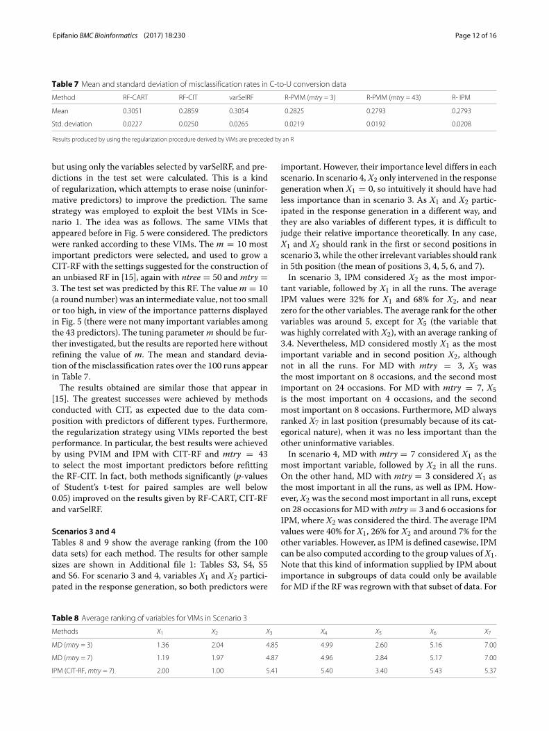
were averaged, and are displayed by barplots in Fig. 5.The results are similar to those in [15], although withsome slight differences. As in [14, 15], position -1 wasvery important, followed by position 1, which was notdetected in [14]. Note that GVIM, the method with theworst results in Scenario 1, was used in [14]. In [15], fe anddfe were somewhat important (only fe in [14]), but accord-ing to the results with PVIM (mtry = 43) and IPM, cp(more than fe) and fe were somewhat important, but notdfe. Furthermore, according to IPM, there were also twosomewhat important variables: positions -13 and 13.In this real case, we do not know the true impor-

tance pattern of the variables. So, besides the variableimportance study, let us also analyze the predictionaccuracy in this data set. The same scheme as in [15]was considered. The original data were split into a train-ing and test set with a size ratio of 2:1. This procedure wasrepeated 100 times. Each time the following operationswere carried out. A RF-CART with bootstrap samplingwithout replacement, with ntree = 50 and mtry = 3as in [15] was grown using the training set, and obser-vations in the test set were predicted with this RF. Thesame procedure was performed with a CIT-RF with thesettings suggested for the construction of an unbiasedRF in [15], again with ntree = 50 and mtry = 3, as in[15]. These two procedures were used in [15]. On thisoccasion, the variable selection varSelRF was considered(varSelMD was not considered due to the poor resultsobtained in Scenario 1). An RF-CART was built as before,

PV

IM (

mtr

y =

3)

0.00

0.02

0.04

PV

IM (

mtr

y =

43)

0.00

0.04

0.08

0.12

−20

−19

−18

−17

−16

−15

−14

−13

−12

−11

−10 −9

−8

−7

−6

−5

−4

−3

−2

−1 1 2 3 4 5 6 7 8 9 10 11 12 13 14 15 16 17 18 19 20 cp fe dfe

IPM

0.00

0.10

0.20

Fig. 5 VIM barplots for the C-to-U conversion data. The first row corresponds to PVIM-CIT withmtry = 3, the second row tomtry = 43, while thebottom row to IPM-CIT-RF values withmtry = 43. In all cases, values are averaged over 100 replications. The variable names appear at bottom of thebarplots

Epifanio BMC Bioinformatics (2017) 18:230 Page 12 of 16

Table 7 Mean and standard deviation of misclassification rates in C-to-U conversion data

Method RF-CART RF-CIT varSelRF R-PVIM (mtry = 3) R-PVIM (mtry = 43) R- IPM

Mean 0.3051 0.2859 0.3054 0.2825 0.2793 0.2793

Std. deviation 0.0227 0.0250 0.0265 0.0219 0.0192 0.0208

Results produced by using the regularization procedure derived by VIMs are preceded by an R

but using only the variables selected by varSelRF, and pre-dictions in the test set were calculated. This is a kindof regularization, which attempts to erase noise (uninfor-mative predictors) to improve the prediction. The samestrategy was employed to exploit the best VIMs in Sce-nario 1. The idea was as follows. The same VIMs thatappeared before in Fig. 5 were considered. The predictorswere ranked according to these VIMs. The m = 10 mostimportant predictors were selected, and used to grow aCIT-RF with the settings suggested for the construction ofan unbiased RF in [15], again with ntree = 50 andmtry =3. The test set was predicted by this RF. The valuem = 10(a round number) was an intermediate value, not too smallor too high, in view of the importance patterns displayedin Fig. 5 (there were not many important variables amongthe 43 predictors). The tuning parameterm should be fur-ther investigated, but the results are reported here withoutrefining the value of m. The mean and standard devia-tion of the misclassification rates over the 100 runs appearin Table 7.The results obtained are similar those that appear in

[15]. The greatest successes were achieved by methodsconducted with CIT, as expected due to the data com-position with predictors of different types. Furthermore,the regularization strategy using VIMs reported the bestperformance. In particular, the best results were achievedby using PVIM and IPM with CIT-RF and mtry = 43to select the most important predictors before refittingthe RF-CIT. In fact, both methods significantly (p-valuesof Student’s t-test for paired samples are well below0.05) improved on the results given by RF-CART, CIT-RFand varSelRF.

Scenarios 3 and 4Tables 8 and 9 show the average ranking (from the 100data sets) for each method. The results for other samplesizes are shown in Additional file 1: Tables S3, S4, S5and S6. For scenario 3 and 4, variables X1 and X2 partici-pated in the response generation, so both predictors were

important. However, their importance level differs in eachscenario. In scenario 4, X2 only intervened in the responsegeneration when X1 = 0, so intuitively it should have hadless importance than in scenario 3. As X1 and X2 partic-ipated in the response generation in a different way, andthey are also variables of different types, it is difficult tojudge their relative importance theoretically. In any case,X1 and X2 should rank in the first or second positions inscenario 3, while the other irrelevant variables should rankin 5th position (the mean of positions 3, 4, 5, 6, and 7).In scenario 3, IPM considered X2 as the most impor-

tant variable, followed by X1 in all the runs. The averageIPM values were 32% for X1 and 68% for X2, and nearzero for the other variables. The average rank for the othervariables was around 5, except for X5 (the variable thatwas highly correlated with X2), with an average ranking of3.4. Nevertheless, MD considered mostly X1 as the mostimportant variable and in second position X2, althoughnot in all the runs. For MD with mtry = 3, X5 wasthe most important on 8 occasions, and the second mostimportant on 24 occasions. For MD with mtry = 7, X5is the most important on 4 occasions, and the secondmost important on 8 occasions. Furthermore, MD alwaysranked X7 in last position (presumably because of its cat-egorical nature), when it was no less important than theother uninformative variables.In scenario 4, MD with mtry = 7 considered X1 as the

most important variable, followed by X2 in all the runs.On the other hand, MD with mtry = 3 considered X1 asthe most important in all the runs, as well as IPM. How-ever, X2 was the second most important in all runs, excepton 28 occasions for MDwithmtry= 3 and 6 occasions forIPM, where X2 was considered the third. The average IPMvalues were 40% for X1, 26% for X2 and around 7% for theother variables. However, as IPM is defined casewise, IPMcan be also computed according to the group values of X1.Note that this kind of information supplied by IPM aboutimportance in subgroups of data could only be availablefor MD if the RF was regrown with that subset of data. For

Table 8 Average ranking of variables for VIMs in Scenario 3

Methods X1 X2 X3 X4 X5 X6 X7

MD (mtry = 3) 1.36 2.04 4.85 4.99 2.60 5.16 7.00

MD (mtry = 7) 1.19 1.97 4.87 4.96 2.84 5.17 7.00

IPM (CIT-RF,mtry = 7) 2.00 1.00 5.41 5.40 3.40 5.43 5.37

Epifanio BMC Bioinformatics (2017) 18:230 Page 13 of 16

Table 9 Average ranking of variables for VIMs in Scenario 4

Methods X1 X2 X3 X4 X5 X6 X7

MD (mtry = 3) 1.00 2.28 5.07 4.97 2.74 4.94 7.00

MD (mtry = 7) 1.00 2.00 4.91 5.02 3.22 4.85 7.00

IPM (CIT-RF,mtry = 7) 1.00 2.06 4.59 4.71 6.11 4.75 4.78

samples with X1 = 0, the average IPM values were 47% forX1 and 53% for X2. Remember that when X1 = 0, the vari-able X2 intervened in the generation of the responses. Forsamples with X1 = 1 (X2 did not intervene in the gener-ation of the responses), the average IPM values were 35%for X1, 7% for X2, 13% for X3, 13% for X4, 6% for X5, 13%for X6 and 12% for X7. Note that when X1 = 1, neitherof the variables intervened in the model generation, so allthe variables were equally unimportant. The selection fre-quency with CIT should be similar [15]. The sum of IPMof the two correlated variables X2 and X5 was 13%. Notealso that this situation, where neither of the predictors isrelated with responses, is not expected (nor desirable) inpractice.

Application to a nutrigenomic studyLet us first analyze the VIMs. As the response is mul-tivariate, only MD and IPM-CIT-RF can be computed.This problem is placed in a high-dimensional setting: itdeals with large p (122) and small n (40). As explainedin [10], as p increases, the tree becomes overwhelmedwith variables, so trees will be too shallow. If we com-pute varSelMD and IPM-CIT-RF with mtry = 122 andntree = 1000, only the variable diet is selected in bothcases. This solution could be viewed as a ’degenerate’solution. Then, the default mtry value in function rfsrcfrom R package randomForestSRC [20] is used. In thiscase mtry = p/3 (rounded up), i.e. mtry = 41. A totalof 34 variables were selected by varSelMD, diet beingthe least deep and genotype being the fourth least deep.However, except for diet, the depth values were notvery different. To provide stability, this procedure wasrepeated 100 times with different seeds. A total of 44variables were selected in some of the replicates. Halfof these, 22 variables, were selected in all the replicatesand 27 of them were selected on more than 75% ofoccasions. In particular, these were the following 27predictors (the number of times they were selectedover the 100 replicates is given in brackets): ACAT2(100), ACBP (100), ACC2 (100), ACOTH (100),apoC3 (100), BSEP (89), CAR1 (100), CYP2c29 (100),

CYP3A11 (100), CYP4A10 (100), CYP4A14 (100), diet(100), G6Pase (96), genotype (100), GK (77), GSTpi2(100), HPNCL (100), Lpin (100), Lpin1 (100), Lpin2 (97),Ntcp (100), PLTP (100), PMDCI (100), S14 (100), SPI1.1(100), SR.BI (99), and THIOL (100).For the 100 replicates of IPM-CIT-RF with mtry = 41,

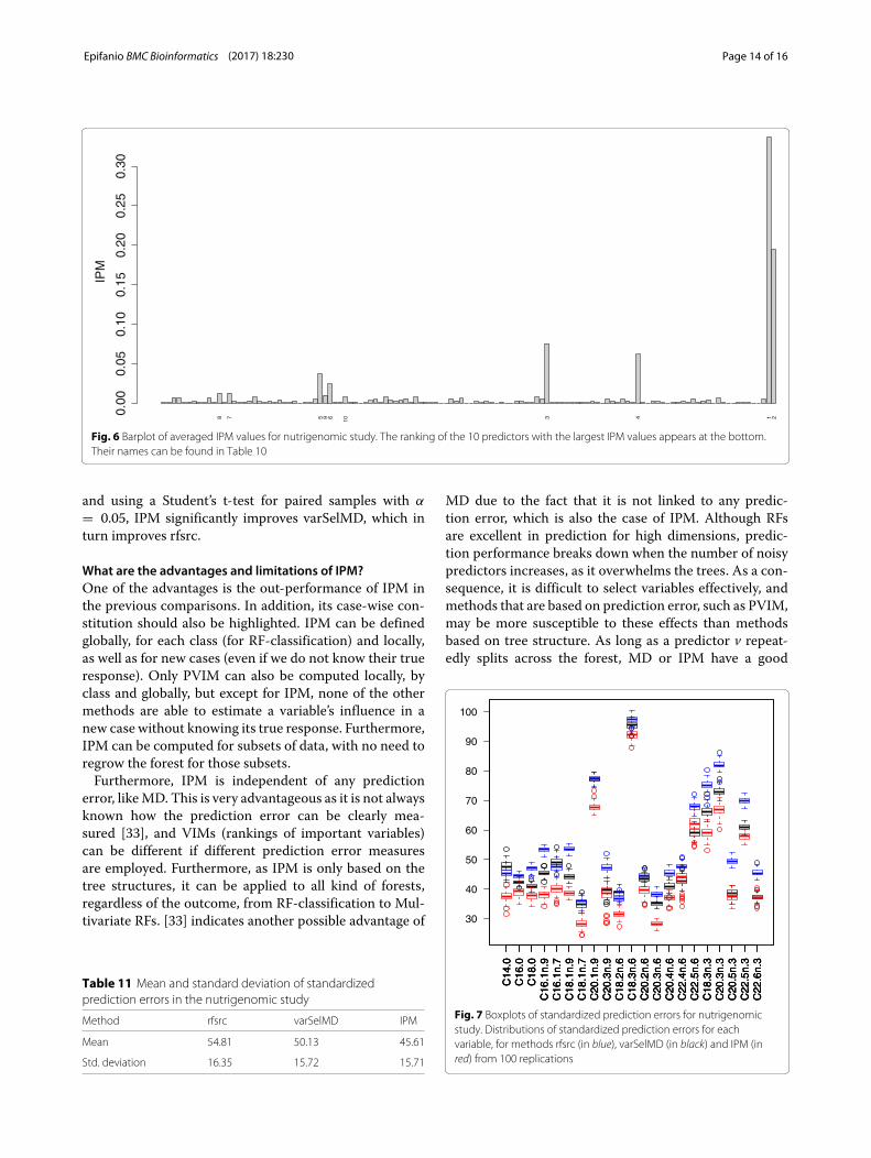
the ranking of the first variables was very stable: dietwas the first in all replicates, and genotype the second.The average ranking of the first ten ranked predictorstogether with the standard deviation for the 100 repli-cates can be seen in Table 10. Although not suggestedby the varSelMD results, the IPM values indicate thatfour variables accounted for most relevance (nearly 70%).In particular, these are the averaged IPM values for thefour variables in brackets: diet (33.7%), genotype (19.5%),PMDCI (7.5%) and THIOL (6.2%). The barplot of theseIPM values can be seen in Fig. 6. The seventh and eightmost important predictors according to IPM, BIEN andAOX were not selected in any of the replications ofvarSelMD.Let us analyze the prediction performance. Prediction

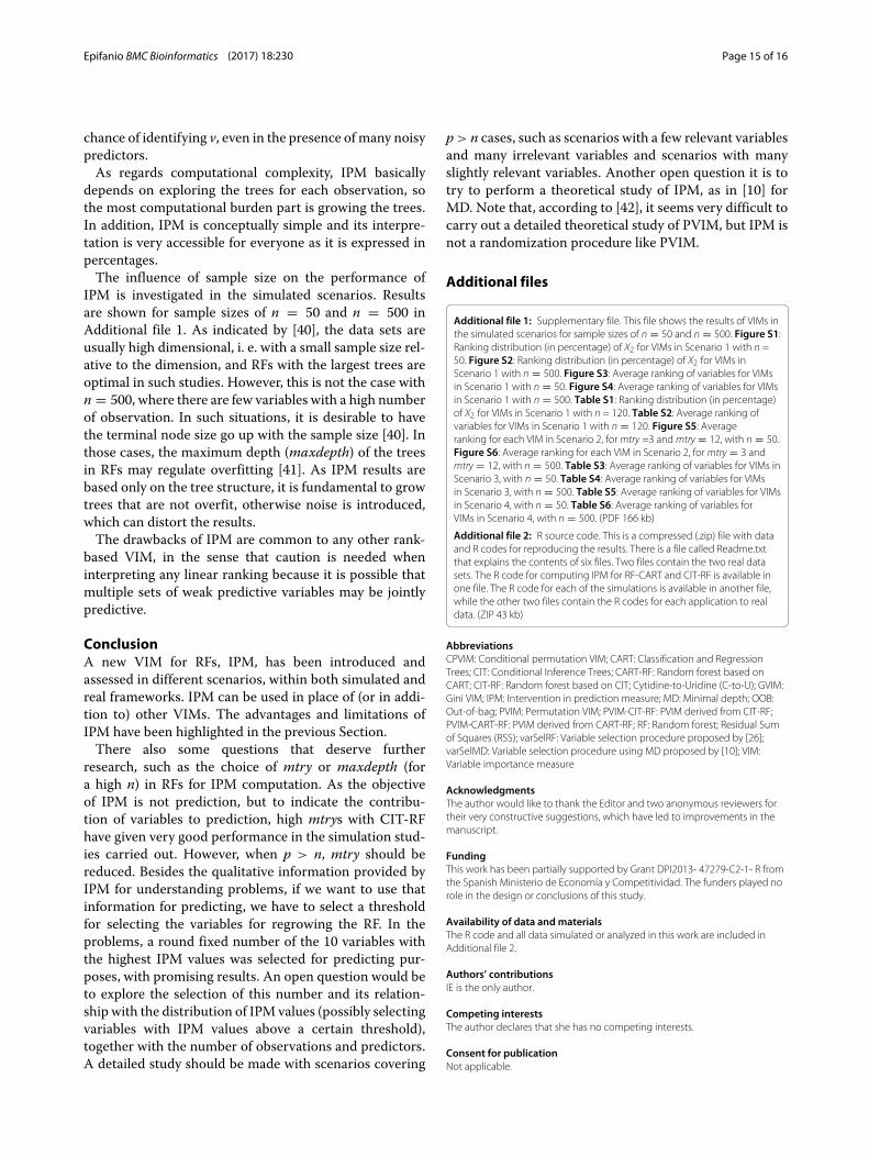
error was calculated using OOB data. As the responseswere continuous, performance was measured in termsof mean-squared-error. The prediction error for eachof the 21 responses was standardized (dividing by thevariance as in the R package randomForestSRC [20])for proper comparison. The prediction error using thefunction rfsrc from R package randomForestSRC withthe default values was computed, which is referred toas rfsrc. varSelMD was applied as before, and the func-tion rfsrc was again used for prediction afterwards, butthe selected variables were used as input instead allthe variables. This procedure is referred as varSelMD.Finally, instead of varSelMD, IPM-CIT-RF was applied asbefore, and the 10most important variables were selected,for prediction. This procedure was referred as IPM.The standardized errors for each response were aver-aged over 100 independent experiments, and their resultsare summarized in Table 11 and displayed in Fig. 7. Thelower prediction errors from IPM can be clearly observed.Furthermore, by pooling the samples for each variable

Table 10 Average ranking of the first 10 ranked variables in the nutrigenomic study for IPM (SD in brackets)

diet genotype PMDCI THIOL CYP3A11 CYP4A14 BIEN AOX CYP4A10 FAS

1 (0) 2 (0) 3.1 (0.3) 3.9 (0.4) 5 (0.2) 6.1 (0.8) 9.1 (3.6) 9.1 (3) 12.4 (5.2) 17 (8.6)

Epifanio BMC Bioinformatics (2017) 18:230 Page 14 of 16

8 7 5 9 6 10 3 4 1 2

IPM

0.00

0.05

0.10

0.15

0.20

0.25

0.30

Fig. 6 Barplot of averaged IPM values for nutrigenomic study. The ranking of the 10 predictors with the largest IPM values appears at the bottom.Their names can be found in Table 10

and using a Student’s t-test for paired samples with α

= 0.05, IPM significantly improves varSelMD, which inturn improves rfsrc.

What are the advantages and limitations of IPM?One of the advantages is the out-performance of IPM inthe previous comparisons. In addition, its case-wise con-stitution should also be highlighted. IPM can be definedglobally, for each class (for RF-classification) and locally,as well as for new cases (even if we do not know their trueresponse). Only PVIM can also be computed locally, byclass and globally, but except for IPM, none of the othermethods are able to estimate a variable’s influence in anew case without knowing its true response. Furthermore,IPM can be computed for subsets of data, with no need toregrow the forest for those subsets.Furthermore, IPM is independent of any prediction

error, likeMD. This is very advantageous as it is not alwaysknown how the prediction error can be clearly mea-sured [33], and VIMs (rankings of important variables)can be different if different prediction error measuresare employed. Furthermore, as IPM is only based on thetree structures, it can be applied to all kind of forests,regardless of the outcome, from RF-classification to Mul-tivariate RFs. [33] indicates another possible advantage of

Table 11 Mean and standard deviation of standardizedprediction errors in the nutrigenomic study

Method rfsrc varSelMD IPM

Mean 54.81 50.13 45.61

Std. deviation 16.35 15.72 15.71

MD due to the fact that it is not linked to any predic-tion error, which is also the case of IPM. Although RFsare excellent in prediction for high dimensions, predic-tion performance breaks down when the number of noisypredictors increases, as it overwhelms the trees. As a con-sequence, it is difficult to select variables effectively, andmethods that are based on prediction error, such as PVIM,may be more susceptible to these effects than methodsbased on tree structure. As long as a predictor v repeat-edly splits across the forest, MD or IPM have a good

C14

.0C

16.0

C18

.0C

16.1

n.9

C16

.1n.

7C

18.1

n.9

C18

.1n.

7C

20.1

n.9

C20

.3n.

9C

18.2

n.6

C18

.3n.

6C

20.2

n.6

C20

.3n.

6C

20.4

n.6

C22

.4n.

6C

22.5

n.6

C18

.3n.

3C

20.3

n.3

C20

.5n.

3C

22.5

n.3

C22

.6n.

3

C14

.0C

16.0

C18

.0C

16.1

n.9

C16

.1n.

7C

18.1

n.9

C18

.1n.

7C

20.1

n.9

C20

.3n.

9C

18.2

n.6

C18

.3n.

6C

20.2

n.6

C20

.3n.

6C

20.4

n.6

C22

.4n.

6C

22.5

n.6

C18

.3n.

3C

20.3

n.3

C20

.5n.

3C

22.5

n.3

C22

.6n.

3

C14

.0C

16.0

C18

.0C

16.1

n.9

C16

.1n.

7C

18.1

n.9

C18

.1n.

7C

20.1

n.9

C20

.3n.

9C

18.2

n.6

C18

.3n.

6C

20.2

n.6

C20

.3n.

6C

20.4

n.6

C22

.4n.

6C

22.5

n.6

C18

.3n.

3C

20.3

n.3

C20

.5n.

3C

22.5

n.3

C22

.6n.

3

30

40

50

60

70

80

90

100

Fig. 7 Boxplots of standardized prediction errors for nutrigenomicstudy. Distributions of standardized prediction errors for eachvariable, for methods rfsrc (in blue), varSelMD (in black) and IPM (inred) from 100 replications

Epifanio BMC Bioinformatics (2017) 18:230 Page 15 of 16

chance of identifying v, even in the presence of many noisypredictors.As regards computational complexity, IPM basically

depends on exploring the trees for each observation, sothe most computational burden part is growing the trees.In addition, IPM is conceptually simple and its interpre-tation is very accessible for everyone as it is expressed inpercentages.The influence of sample size on the performance of

IPM is investigated in the simulated scenarios. Resultsare shown for sample sizes of n = 50 and n = 500 inAdditional file 1. As indicated by [40], the data sets areusually high dimensional, i. e. with a small sample size rel-ative to the dimension, and RFs with the largest trees areoptimal in such studies. However, this is not the case withn = 500, where there are few variables with a high numberof observation. In such situations, it is desirable to havethe terminal node size go up with the sample size [40]. Inthose cases, the maximum depth (maxdepth) of the treesin RFs may regulate overfitting [41]. As IPM results arebased only on the tree structure, it is fundamental to growtrees that are not overfit, otherwise noise is introduced,which can distort the results.The drawbacks of IPM are common to any other rank-

based VIM, in the sense that caution is needed wheninterpreting any linear ranking because it is possible thatmultiple sets of weak predictive variables may be jointlypredictive.

ConclusionA new VIM for RFs, IPM, has been introduced andassessed in different scenarios, within both simulated andreal frameworks. IPM can be used in place of (or in addi-tion to) other VIMs. The advantages and limitations ofIPM have been highlighted in the previous Section.There also some questions that deserve further

research, such as the choice of mtry or maxdepth (fora high n) in RFs for IPM computation. As the objectiveof IPM is not prediction, but to indicate the contribu-tion of variables to prediction, high mtrys with CIT-RFhave given very good performance in the simulation stud-ies carried out. However, when p > n, mtry should bereduced. Besides the qualitative information provided byIPM for understanding problems, if we want to use thatinformation for predicting, we have to select a thresholdfor selecting the variables for regrowing the RF. In theproblems, a round fixed number of the 10 variables withthe highest IPM values was selected for predicting pur-poses, with promising results. An open question would beto explore the selection of this number and its relation-ship with the distribution of IPM values (possibly selectingvariables with IPM values above a certain threshold),together with the number of observations and predictors.A detailed study should be made with scenarios covering

p> n cases, such as scenarios with a few relevant variablesand many irrelevant variables and scenarios with manyslightly relevant variables. Another open question it is totry to perform a theoretical study of IPM, as in [10] forMD. Note that, according to [42], it seems very difficult tocarry out a detailed theoretical study of PVIM, but IPM isnot a randomization procedure like PVIM.

Additional files

Additional file 1: Supplementary file. This file shows the results of VIMs inthe simulated scenarios for sample sizes of n = 50 and n = 500. Figure S1:Ranking distribution (in percentage) of X2 for VIMs in Scenario 1 with n =50. Figure S2: Ranking distribution (in percentage) of X2 for VIMs inScenario 1 with n = 500. Figure S3: Average ranking of variables for VIMsin Scenario 1 with n = 50. Figure S4: Average ranking of variables for VIMsin Scenario 1 with n = 500. Table S1: Ranking distribution (in percentage)of X2 for VIMs in Scenario 1 with n = 120. Table S2: Average ranking ofvariables for VIMs in Scenario 1 with n = 120. Figure S5: Averageranking for each VIM in Scenario 2, formtry =3 andmtry = 12, with n = 50.Figure S6: Average ranking for each VIM in Scenario 2, formtry = 3 andmtry = 12, with n = 500. Table S3: Average ranking of variables for VIMs inScenario 3, with n = 50. Table S4: Average ranking of variables for VIMsin Scenario 3, with n = 500. Table S5: Average ranking of variables for VIMsin Scenario 4, with n = 50. Table S6: Average ranking of variables forVIMs in Scenario 4, with n = 500. (PDF 166 kb)

Additional file 2: R source code. This is a compressed (.zip) file with dataand R codes for reproducing the results. There is a file called Readme.txtthat explains the contents of six files. Two files contain the two real datasets. The R code for computing IPM for RF-CART and CIT-RF is available inone file. The R code for each of the simulations is available in another file,while the other two files contain the R codes for each application to realdata. (ZIP 43 kb)

AbbreviationsCPVIM: Conditional permutation VIM; CART: Classification and RegressionTrees; CIT: Conditional Inference Trees; CART-RF: Random forest based onCART; CIT-RF: Random forest based on CIT; Cytidine-to-Uridine (C-to-U); GVIM:Gini VIM; IPM: Intervention in prediction measure; MD: Minimal depth; OOB:Out-of-bag; PVIM: Permutation VIM; PVIM-CIT-RF: PVIM derived from CIT-RF;PVIM-CART-RF: PVIM derived from CART-RF; RF: Random forest; Residual Sumof Squares (RSS); varSelRF: Variable selection procedure proposed by [26];varSelMD: Variable selection procedure using MD proposed by [10]; VIM:Variable importance measure

AcknowledgmentsThe author would like to thank the Editor and two anonymous reviewers fortheir very constructive suggestions, which have led to improvements in themanuscript.

FundingThis work has been partially supported by Grant DPI2013- 47279-C2-1- R fromthe Spanish Ministerio de Economía y Competitividad. The funders played norole in the design or conclusions of this study.

Availability of data andmaterialsThe R code and all data simulated or analyzed in this work are included inAdditional file 2.

Authors’ contributionsIE is the only author.

Competing interestsThe author declares that she has no competing interests.

Consent for publicationNot applicable.

Epifanio BMC Bioinformatics (2017) 18:230 Page 16 of 16

Ethics approval and consent to participateNot applicable.

Publisher’s NoteSpringer Nature remains neutral with regard to jurisdictional claims inpublished maps and institutional affiliations.

Received: 13 January 2017 Accepted: 25 April 2017

References1. Hastie T, Tibshirani R, Friedman J. The Elements of Statistical Learning.

Data Mining, Inference and Prediction, 2nd ed. New York: Springer-Verlag;2009.

2. Breiman L. Random forests. Mach Learn. 2001;45(1):5–32.3. Segal M, Xiao Y. Multivariate random forests. Wiley Interdiscip Rev Data

Min Knowl Discov. 2011;1(1):80–7.4. Boulesteix AL, Janitza S, Kruppa J, König IR. Overview of random forest

methodology and practical guidance with emphasis on computationalbiology and bioinformatics. Wiley Interdiscip Rev Data Min Knowl Discov.2012;2(6):493–507.

5. Chen X, Ishwaran H. Random forests for genomic data analysis.Genomics. 2012;99(6):323–9. doi:10.1016/j.ygeno.2012.04.003.

6. Xiao Y, Segal M. Identification of yeast transcriptional regulationnetworks using multivariate random forests. PLoS Comput Biol. 2009;5(6):1–18. doi:10.1371/journal.pcbi.1000414.

7. Wei P, Lu Z, Song J. Variable importance analysis: A comprehensivereview. Reliab Eng Syst Saf. 2015;142:399–432.

8. Steyerberg E, Vickers A, Cook N, Gerds T, Gonen M, Obuchowski N,Pencina M, Kattan M. Assessing the performance of prediction models: aframework for some traditional and novel measures. Epidemiology.2010;21(1):128–38.

9. Janitza S, Strobl C, Boulesteix AL. An AUC-based permutation variableimportance measure for random forests. BMC Bioinformatics. 2013;14(1):119. doi:10.1186/1471-2105-14-119.

10. Ishwaran H, Kogalur U, Gorodeski E, Minn A, Lauer M. High-dimensionalvariable selection for survival data. J Am Stat Assoc. 2010;105(489):205–17.

11. Pierola A, Epifanio I, Alemany S. An ensemble of ordered logisticregression and random forest for child garment size matching. ComputInd Eng. 2016;101:455–65.

12. Breiman L, Friedman JH, Olshen RA, Stone CJ. Classification andregression trees. Stat Probab Series. Belmont: Wadsworth PublishingCompany; 1984.

13. Hothorn T, Hornik K, Zeileis A. Unbiased recursive partitioning: Aconditional inference framework. J Comput Graph Stat. 2006;15(3):651–74.

14. Cummings MP, Myers DS. Simple statistical models predict C-to-U editedsites in plant mitochondrial RNA. BMC Bioinformatics. 2004;5(1):132.doi:10.1186/1471-2105-5-132.

15. Strobl C, Boulesteix AL, Zeileis A, Hothorn T. Bias in random forestvariable importance measures: Illustrations, sources and a solution. BMCBioinformatics. 2007;8(1):25. doi:10.1186/1471-2105-8-25.

16. Martin PGP, Guillou H, Lasserre F, Déjean S, Lan A, Pascussi JM,SanCristobal M, Legrand P, Besse P, Pineau T. Novel aspects ofpparα-mediated regulation of lipid and xenobiotic metabolism revealedthrough a nutrigenomic study. Hepatology. 2007;45(3):767–77.doi:10.1002/hep.21510.

17. R Development Core Team. R: A Language and Environment for StatisticalComputing. Vienna: R Foundation for Statistical Computing; 2016. http://www.R-project.org/.

18. Breiman L, Cutler A, Liaw A, Wiener M. Breiman and Cutler’s RandomForests for Classification and Regression. 2015. R package version 4.6.12.https://cran.r-project.org/package=randomForest. Accessed 12 Jan 2017.

19. Liaw A, Wiener M. Classification and regression by randomforest. R News.2002;2(3):18–22.

20. Ishwaran H, Kogalur UB. Random Forests for Survival, Regression andClassification (RF-SRC). 2016. R package version 2.4.1. https://cran.r-project.org/package=randomForestSRC. Accessed 12 Jan 2017.

21. Ishwaran H, Kogalur UB. Random survival forests for r. R News. 2007;7(2):25–31.

22. Ishwaran H, Kogalur UB, Blackstone EH, Lauer MS. Random survivalforests. Ann Appl Stat. 2008;2(3):841–60.

23. Hothorn T, Hornik K, Strobl C, Zeileis A. A Laboratory for RecursivePartytioning. 2016. R package version 1.0.25. https://cran.r-project.org/package=party. Accessed 12 Jan 2017.

24. Hothorn T, Buehlmann P, Dudoit S, Molinaro A, Van Der Laan M. Survivalensembles. Biostatistics. 2006;7(3):355–73.

25. Strobl C, Boulesteix AL, Kneib T, Augustin T, Zeileis A. Conditionalvariable importance for random forests. BMC Bioinformatics. 2008;9(1):307. doi:10.1186/1471-2105-9-307.

26. Díaz-Uriarte R, Alvarez de Andrés S. Gene selection and classification ofmicroarray data using random forest. BMC Bioinformatics. 2006;7(1):3.doi:10.1186/1471-2105-7-3.

27. Díaz-Uriarte R. Variable Selection Using Random Forests. 2016. R packageversion 0.7.5. https://cran.r-project.org/package=varSelRF. Accessed 12Jan 2017.

28. Díaz-Uriarte R. Genesrf and varselrf: a web-based tool and r package forgene selection and classification using random forest. BMCBioinformatics. 2007;8(1):328. doi:10.1186/1471-2105-8-328.

29. Strobl C, Zeileis A. Danger: High power! – Exploring the statisticalproperties of a test for random forest variable importance. In: Brito P,editor. COMPSTAT 2008 – Proceedings in Computational Statistics, vol. II.Heidelberg: Physica Verlag; 2008. p. 59–66. https://eeecon.uibk.ac.at/~zeileis/papers/Strobl+Zeileis-2008.pdf.

30. Breiman L, Cutler A. Random Forests. 2004. http://www.stat.berkeley.edu/~breiman/RandomForests/. Accessed 12 Jan 2017.

31. Nicodemus KK, Malley JD, Strobl C, Ziegler A. The behaviour of randomforest permutation-based variable importance measures under predictorcorrelation. BMC Bioinformatics. 2010;11(1):110. doi:10.1186/1471-2105-11-110.

32. Boulesteix AL, Janitza S, Hapfelmeier A, Van Steen K, Strobl C. Letter tothe editor: On the term ‘interaction’ and related phrases in the literatureon random forests. Brief Bioinform. 2015;16(2):338–45.doi:10.1093/bib/bbu012.

33. Ishwaran H, Kogalur UB, Chen X, Minn AJ. Random survival forests forhigh-dimensional data. Stat Anal Data Mining. 2011;4(1):115–32.doi:10.1002/sam.10103.

34. Hapfelmeier A, Hothorn T, Ulm K, Strobl C. A new variable importancemeasure for random forests with missing data. Stat Comput. 2014;24(1):21–34. doi:10.1007/s11222-012-9349-1.

35. Kendall MG. Rank Correlation Methods. Oxford: C. Griffin; 1948.36. Gamer M, Lemon J, Singh IFP. Irr: Various Coefficients of Interrater

Reliability and Agreement. 2012. R package version 0.84. http://CRAN.R-project.org/package=irr. Accessed 12 Jan 2017.

37. Touw WG, Bayjanov JR, Overmars L, Backus L, Boekhorst J, Wels M,Hijum SAFT. Data mining in the life sciences with random forest: a walk inthe park or lost in the jungle Brief Bioinform. 2013;14(3):315–26.doi:10.1093/bib/bbs034.

38. Wuchty S, Arjona D, Li A, Kotliarov Y, Walling J, Ahn S, Zhang A, Maric D,Anolik R, Zenklusen JC, Fine HA. Prediction of associations betweenmicroRNAs and gene expression in glioma biology. PLOS ONE. 2011;6(2):1–10. doi:10.1371/journal.pone.0014681.

39. Bayjanov JR, Molenaar D, Tzeneva V, Siezen RJ, van Hijum SAFT.Phenolink - a web-tool for linking phenotype to ~omics data for bacteria:application to gene-trait matching for Lactobacillus plantarum strains.BMC Genomics. 2012;13(1):170. doi:10.1186/1471-2164-13-170.

40. Lin Y, Jeon Y. Random forests and adaptive nearest neighbors. J Am StatAssoc. 2006;101(474):578–90.

41. Strobl C, Malley J, Tutz G. An introduction to recursive partitioning:Rationale, application, and characteristics of classification and regressiontrees, bagging, and random forests. Psychol Methods. 2009;14(4):323–48.

42. Ishwaran H. Variable importance in binary regression trees and forests.Electron J Stat. 2007;1:519–37. doi:10.1214/07-EJS039.

43. Breiman L. Manual On Setting Up, Using, and Understanding RandomForests V4.0. Statistics Department, University of California, Berkeley.Statistics Department, University of California, Berkeley. 2003. https://www.stat.berkeley.edu/~breiman/Using_random_forests_v4.0.pdf.