methods and metrics for evaluating environmental dredging

0

EPA/600/R-16/322 | October 2016 | www.epa.gov/research

Methods and Metrics for Evaluating Environmental Dredging at the Ashtabula River Area of Concern (AOC)

EPA/600/R-16/322 October 2016

Methods and Metrics for Evaluating Environmental Dredging

at the Ashtabula River Area of Concern (AOC)

by

Battelle Columbus, OH 43201

and

Integral Consulting Inc. Santa Cruz, CA 95060

Contract No. EP-C-05-057 Task Order 50

Contract No. EP-W-09-024

Work Assignments 2-13 and 3-07

Contract No. EP-C-11-038 Task Order 30

Co-Principal Investigators Marc Mills, Richard Brenner, and Joseph Schubauer-Berigan

Land Remediation and Pollution Control Division National Risk Management Research Laboratory

and

James Lazorchak and John Meier (r)

Systems Exposure Division National Exposure Research Laboratory

Office of Research and Development

U.S. Environmental Protection Agency Cincinnati, OH 45268

i

Notice/Disclaimer The U.S. Environmental Protection Agency (EPA), through its Office of Research and Development (ORD), funded and managed, or partially funded and collaborated in, the research described herein. It has been subjected to the Agency’s peer and administrative review and has been approved for publication. Any opinions expressed in this report are those of the authors and do not necessarily reflect the views of the Agency; therefore, no official endorsement should be inferred. Any mention of trade names or commercial products does not constitute endorsement or recommendation for use.

ii

Foreword The U.S. Environmental Protection Agency (U.S. EPA) is charged by Congress with protecting the Nation's land, air, and water resources. Under a mandate of national environmental laws, the Agency strives to formulate and implement actions leading to a compatible balance between human activities and the ability of natural systems to support and nurture life. To meet this mandate, U.S. EPA's research program is providing data and technical support for solving environmental problems today and building a science knowledge base necessary to manage our ecological resources wisely, understand how pollutants affect our health, and prevent or reduce environmental risks in the future. The National Risk Management Research Laboratory (NRMRL) is the Agency's center for investigation of technological and management approaches for preventing and reducing risks from pollution that threaten human health and the environment. The focus of the Laboratory's research program is on methods and their cost-effectiveness for prevention and control of pollution to air, land, water, and subsurface resources; protection of water quality in public water systems; remediation of contaminated sites, sediments and ground water; prevention and control of indoor air pollution; and restoration of ecosystems. NRMRL collaborates with both public and private sector partners to foster technologies that reduce the cost of compliance and to anticipate emerging problems. NRMRL's research provides solutions to environmental problems by: developing and promoting technologies that protect and improve the environment, advancing scientific and engineering information to support regulatory and policy decisions, and providing the technical support and information transfer to ensure implementation of environmental regulations and strategies at the national, state, and community levels. International concern about contaminated sediments is increasing, mainly because sediments are viewed as long-term pollutant sinks for compounds such as polychlorinated biphenyls (PCBs), polycyclic aromatic hydrocarbons (PAHs), metals, and other contaminants of concern (COCs). Large areas of contaminated sediment accumulation are known to pose a threat to benthic, aquatic, and terrestrial ecosystems as well as human health. Sediment contamination exists in every region and state of the Nation, negatively impacting overlying surface waters and surrounding ecosystems. To date, three primary technologies have been applied to the remediation of contaminated sediment sites: 1) engineered capping with imported clean material such as sand, 2) monitored natural recovery (MNR) wherein the contaminant source is known to have been removed and natural capping with indigenous clean sediment is allowed to cover or bury the contaminated sediment over a long period of time, and 3) environmental dredging that relies on rapid mechanical removal of the contaminated sediment layer and subsequent off-site confined disposal. Environmental dredging was selected as the remedy of choice for remediation and cleanup of the Ashtabula River Area of Concern (AOC), a highly contaminated sediment site in northeastern Ohio. PCBs constituted the primary COC for this site, with PAHs and inorganic chemicals comprising secondary COCs. Dredging was carried out from the fall of 2006 through the fall of 2007 on this AOC. The site was extensively characterized in the spring and summer of 2006 prior to the onset of dredging. A comprehensive evaluation and monitoring program conducted by U.S EPA then ensued: 1) during the dredging period, 2) immediately following dredging in early 2008, and 3) over the next 3 years through 2011 to assess long-term recovery. This report summarizes and interprets the results of this 6-year study to monitor pollutant fate

iii

and transport and ecosystem recovery through the use of bathymetry; sampling and chemical analysis of sediment, water, and indigenous fish; and deployment and follow-up retrieval and analysis of macrobenthos and passive samplers.

Cynthia Sonich-Mullin, Director National Risk Management Research Laboratory

iv

Abstract

International concern about contaminated sediments is increasing as sustainable practices are needed to maintain our water resources and waterways as important economic, commercial, recreational, and community resources. Sediments often serve as long-term sinks for legacy pollutants, such as polychlorinated biphenyls (PCBs), polycyclic aromatic hydrocarbons (PAHs), inorganics, and other emerging and known contaminants of concern (COCs). Large areas of contaminated sediment accumulation are known to pose a threat to benthic, aquatic, and terrestrial ecosystems, as well as human health. Sediment contamination exists in every U.S. EPA Region and state of the Nation, negatively impacting overlying surface waters and surrounding ecosystems, and ultimately the health and quality of life for surrounding communities. To date, three primary management strategies have been applied to remediate contaminated sediment sites: 1) engineered caps, 2) monitored natural recovery (MNR), and 3) environmental dredging or a combination of these approaches. Engineered capping relies on the isolation of the contaminant from receptors and, more recently, may incorporate sorptive or reactive media to mitigate or treat contaminants that may migrate through the cap. MNR depends on monitoring to verify the source control actions and natural processes to isolate, degrade, and/or control the release of contaminants are progressing as predicted. Environmental dredging utilizes rapid mechanical removal of the contaminated sediment followed by isolation of the contaminated sediment from potential receptors. Modern sediment remediation generally uses a combination of these strategies to optimize environmental protection and the cost of remediation. U.S. EPA’s Office of Research and Development (ORD) has an interdisciplinary research program to evaluate the effectiveness of risk management strategies and develop innovative treatment technologies. These projects have investigated and documented methods and approaches to assess remediation projects in the short term (project driven goals) and over longer-term restoration and recovery periods (programmatic goals). Research described in this report focuses on the development of methods and approaches to conduct a remedy effectiveness assessment (REA) on environmental remediation projects. In this research effort, several monitoring and sampling approaches were developed, standardized, and demonstrated on a sediment remediation project at the Ashtabula River initiated in 2006 by U.S. EPA’s Great Lakes National Program Office (GLNPO) under the Great Lakes Legacy Act (GLLA). Environmental dredging was utilized on approximately 1.2 miles in a lower reach of this river in northeastern Ohio. PCBs constituted the primary COC for this site, with PAHs and inorganic chemicals comprising secondary COCs. Hydraulic dredging was carried out from the fall of 2006 through the fall of 2007 on this GLLA project. Extensive site characterization was conducted by GLNPO, ORD, and their partners at Federal and State agencies in the spring and summer of 2006 prior to the onset of remediation. In partnership with GLNPO and concurrent with the dredging project, a comprehensive research effort was carried out by ORD on the Ashtabula River to develop assessment and monitoring methods along biological, chemical, and physical lines of evidence (LOEs). These LOEs can be used in a weight of evidence (WOE) framework to assess sediment remedies. Utilization, monitoring, and evaluation of these methods and LOE approach began prior to the onset of

v

environmental dredging of the Ashtabula River in 2006 and continued during and following dredging through 2011. This project report summarizes and interprets the results of this 6-year study to develop and assess methods for monitoring contaminant fate and transport and ecosystem recovery through the use of biological, chemical, and physical assessment methodologies such as: 1) comprehensive sampling of and chemical analysis of contaminants in surface, suspended, and historic sediments; 2) multi-level real time water sampling and analysis of contaminants in the water column during remediation; 3) sampling, chemical analysis, and development of alternative toxicity endpoints for indigenous fish; 4) innovative bathymetry, suspended sediment, and plume monitoring and modeling approaches; 5) multi-purpose macrobenthos collection techniques for determining benthic condition and contaminant exposure; and 6) passive sampler technology and deployment techniques. The results of this project demonstrated that the application of multiple LOEs can be utilized on various spatial and temporal scales to inform a project manager on the short- and long-term impacts of sediment remediation. Using multiple LOE-based metrics and a WOE framework, specific mechanisms and processes can be characterized to quantify the short- and long-term impacts of a selected remedy on the surrounding ecosystem. The objective of this specific research project was to develop and demonstrate selected biological, chemical, and physical monitoring methods that can be integrated and applied on future remediation projects for conducting REAs. As the initial product of this new integrated approach, an REA is currently being prepared for the Ashtabula River project by GLNPO and ORD and will be reported separately.

vi

Acknowledgements The support and participation of many researchers, administrators, and support staff were necessary to carry out a multi-year project of this scope and magnitude. Funding provided by the National Risk Management Research Laboratory (NRMRL) of the U.S. Environmental Protection Agency (U.S. EPA) and the U.S. EPA Great Lakes National Program Office (GLNPO) to enable this project to be conducted is gratefully acknowledged. Collaborative efforts and mutual support between NRMRL, GLNPO, and U.S. EPA’s National Exposure Research Laboratory (NERL) provided a forum for exchanging ideas and concepts and were vital to the success of this project. The partnership and cooperation engendered on this study has already begun to pay dividends on other projects. The excellent service and attention to detail of the project’s contractor, Battelle, simplified and optimized the implementation of complex sampling and analytical programs that generated the project’s large and comprehensive dataset. The cooperation of GLNPO’s dredging contractor, J.F. Brennan Company, Inc., in providing dredge data and welcome advice was essential in relating research field measurements to sediment inventories and dredging operations. The authors of this report, Lisa Lefkovitz, Heather Thurston, Stacy Pala, Eric Foote, Greg Durell, Paul Sokoloff, Matt Fitzpatrick, Jessica Tenzar, John Hardin, and Carlton Hunt from Battelle; Craig Jones and Grace Chang from Integral Consulting, Inc. (a subcontractor to Battelle); and Jason Magalen of HDR, Inc., along with U.S. EPA Co-Principal Investigators Marc Mills 0F

, Richard Brenner, Joseph Schubauer-Berigan, James Lazorchak, and John Meier 1F

wish to express their appreciation to the following individuals for their substantial and valuable contributions to this research undertaking:

Battelle U.S. EPA/NRMRL U.S. EPA/GLNPO Greg Headington Pat Clark Scott Cieniawski

Jim Hicks Terry Lyons Amy Pelka Bob Mandeville Paul McCauley Marc Tuchman Shane Walton Dennis Timberlake

Roger Yeardley

U.S. EPA/NERL J.F. Brennan Company,

Inc. Formerly

The McConnell Group Ken Fritz Mark Binsfeld Brandon Armstrong

Brent Johnson Paul Olander Jason Berninger Paul Wernsing Mark Berninger

Herman Haring Paul Weaver

Corresponding Investigator: [email protected] Now retired from the U.S. Environmental Protection Agency.

vii

Table of Contents Notice/Disclaimer ............................................................................................................................ i Foreword ......................................................................................................................................... ii Abstract .......................................................................................................................................... iv Acknowledgements ........................................................................................................................ vi List of Figures ................................................................................................................................ ix List of Tables ................................................................................................................................ xv List of Appendices ....................................................................................................................... xvi Acronyms and Abbreviations ..................................................................................................... xvii 1.0 Introduction ............................................................................................................................. 1

1.1 Description of Project Area .......................................................................................... 3 1.2 Project Goals and Objectives ........................................................................................ 3 1.3 Project Summary ........................................................................................................... 4

2.0 Experimental Approach ......................................................................................................... 11

2.1 Sediment Mapping ...................................................................................................... 11 2.1.1 Bathymetry .................................................................................................. 11 2.1.2 Sidescan Sonar ............................................................................................. 12

2.2 Plume Tracking ........................................................................................................... 12 2.3 Sediment ..................................................................................................................... 16

2.3.1 Sediment Cores ............................................................................................ 16 2.4 Passive Samplers ......................................................................................................... 19

2.4.1 Passive Samplers: Semipermeable Membrane Device ................................ 20 2.4.2 Passive Samplers: Solid Phase Micro-Extraction ........................................ 27

2.5 Macrobenthos Sample Collection ............................................................................... 28 2.6 Caged Clams and Worms............................................................................................ 32 2.7 Indigenous Fish ........................................................................................................... 32 2.8 Chemical and Physical Analytical Methods ............................................................... 33

2.8.1 Chemical and Physical Analysis of Sediment Samples .............................. 33 2.8.2 Chemical Analysis of Water Samples ......................................................... 34 2.8.3 Chemical Analysis of Tissue Samples......................................................... 35 2.8.4 Chemical Analysis of Passive Samplers ...................................................... 36

2.9 Data Management and Data Evaluation ..................................................................... 36 2.10 Quality Assurance/Quality Control............................................................................. 39

3.0 Results ................................................................................................................................... 42

3.1 Bathymetry .................................................................................................................. 42 3.2 Resuspension Survey during Dredging ....................................................................... 47

3.2.1 Plume Tracking ........................................................................................... 47 3.2.2 Resuspended Sediment Mass....................................................................... 62 3.2.3 Link to Contaminant Distribution................................................................ 69

3.3 Sediment ..................................................................................................................... 74 3.3.1 Comparison of tPCB(c) Concentrations in Pre- and Post-Dredge Cores .. 75 3.3.2 Surface Sediment PCBs Trends ................................................................... 84

viii

3.3.3 General Surface Sediment PCB Trends ...................................................... 93 3.4 Biological Samplers .................................................................................................. 104

3.4.1 Macrobenthos Tissue and Co-located Sediment and Water Chemical Results .................................................................................................................. 104

3.4.2 Indigenous Brown Bullhead ...................................................................... 126 3.4.3 PCB Results in Indigenous Brown Bullhead Fish ..................................... 126 3.4.4 PAH Results in Indigenous Brown Bullhead Fish .................................... 128

3.5 Passive Samplers as Biological Surrogates............................................................... 132 3.5.1 Water Column SPMDs .............................................................................. 133 3.5.2 Sediment SPMDs ....................................................................................... 141 3.5.3 Solid Phase Microextraction Devices ........................................................ 148

4.0 Discussion ........................................................................................................................... 155

4.1 Macrobenthos Tissue Concentrations using Artificial Substrate Samplers .............. 155 4.1.1 Macrobenthos ANOVA ............................................................................. 157 4.1.2 Macrobenthos PCA ................................................................................... 162 4.1.3 ANOVA Analysis of Surface Sediment for Macrobenthos Stations ......... 164 4.1.4 Surface Sediment PCA .............................................................................. 166 4.1.5 Macrobenthos Water ANOVA .................................................................. 167 4.1.6 PCA for Waters from Macrobenthos Stations ........................................... 169 4.1.7 Comparison of Macrobenthos Tissue and Co-located Sediment and Water

PCBs ......................................................................................................... 169 4.2 SPMDs ................................................................................................................... 172

4.2.1 Correlation between SPMDs and Co-Located Sediments and Waters ...... 173 4.2.2 Water Column SPMD ANOVA ................................................................ 176

4.3 Indigenous Fish ......................................................................................................... 178 4.3.1 ANOVA for Fish Tissue Chemistry .......................................................... 179 4.3.2 PCA for Fish .............................................................................................. 181

5.0 Conclusions ......................................................................................................................... 183

5.1 Water Sampling during Dredging – Turbidity Measurements ................................. 183 5.2 Water Sampling during Dredging– Resuspended Sediment Mass Measurements ... 185 5.3 Water Sampling during Dredging – Link to Contaminant Distributions .................. 186 5.4 Contaminants in Surface Sediment ........................................................................... 187 5.5 Macrobenthos ............................................................................................................ 188 5.6 Indigenous Fish Tissue Contaminant Concentrations – Brown Bullhead ................ 188 5.7 Semipermeable Membrane Device (SPMD) ............................................................ 190 5.8 Summary ................................................................................................................... 191

6.0 References ........................................................................................................................... 192

ix

List of Figures Figure 1-1. Location of the Ashtabula River Environmental Dredging Project in Ashtabula,

OH. .......................................................................................................................... 2 Figure 1-2. Ashtabula River Dredging Project and ORD Study Area (River Stations 181+00

to 170+00). .............................................................................................................. 2

Figure 2-1. June 2007 Survey Whole Water Sample Collection Locations and Dredge Positions of the Michael B. ................................................................................... 14

Figure 2-2. July 2007 Survey Whole Water Sample Locations and Dredge Positions of the Michael B. (“MB”) and the Palm Beach (“PB”). ................................................. 15

Figure 2-3. Sediment Core Sample Locations in the Ashtabula River Residual Study Area for Pre- (2006) and Post- (2007, 2009, and 2011) Dredging, respectively. ............... 17

Figure 2-4. Sediment SPMD Deployment Locations. ............................................................. 21

Figure 2-5. Water Column SPMD Deployment Locations. .................................................... 22 Figure 2-6. Typical SPMD Rack Design for Deployment of SPMDs on the Surficial

Sediment. .............................................................................................................. 23 Figure 2-7. Top View and Angle View of the SPMD Spider Carrier (EST, St. Joseph, MO). 23

Figure 2-8. Full View and Cross-Sectional View of the Perforated Stainless Steel Carrier with Five Spiders. ......................................................................................................... 24

Figure 2-9. Macrobenthos Samplers Used at Ashtabula River (Left –H-D artificial substrate plate sampler; Right – Samplers hanging in fish cages during deployment). ....... 29

Figure 2-10. Macrobenthos Deployment at the Ashtabula River and Conneaut Creek Reference Site Locations (inset shows Conneaut Creek Reference Location). ..................... 30

Figure 3-1. Pre-Dredge Bathymetric Survey. .......................................................................... 43 Figure 3-2. Bathymetric Differences in meters between 2007 and 2009 for the ORD Study

Area of the Ashtabula River Showing Sediment Coring Locations. .................... 44

Figure 3-3. Bathymetric Differences in meters between 2007 and 2011 for the ORD Study Area of the Ashtabula River Showing Sediment Coring Locations. .................... 45

Figure 3-4. Schematic Depicting the Stationary Turbidity Probe and ADCP Upstream and Downstream of Dredging Activities. .................................................................... 48

Figure 3-5. Dredging Region on the Ashtabula River and Fixed Monitoring Station Locations................................................................................................................................ 49

Figure 3-6. Histograms to Determine Frequency of Occurrence for Turbidity (A), and TSS (B). ........................................................................................................................ 50

Figure 3-7. Up-looking Acoustic Doppler Current Profiler (ADCP) (Teledyne RD Instruments 1200 kHz Workhorse Sentinel ADCP [Poway, CA]) on Bottom-Mount Platform for Measuring TSS. .................................................................... 51

Figure 3-8. Log-linear Relationship between ABS and TSS. .................................................. 51

Figure 3-9. A: Depth-Resolved Time Series of TSSABS.m Derived from ABS Computed from Echo Intensity Measured by the Upstream (South) Bottom-Mounted ADCP. ..... 52

Figure 3-10. A: Depth-Resolved Time Series of TSSABS.m Derived from ABS Computed from Echo Intensity Measured by the Downstream (North) Bottom-Mounted ADCP. 53

Figure 3-11. Time Series of TSS Derived from Optical Turbidity (blue) and Acoustical Backscatter (ABS; red) for Data Collected at the Upstream (South) Site Comparing Methods at about (A) 1 m below the Surface and (B) 1 m above the Bottom and for Data Collected at the Downstream (North) Site Comparing

x

Methods at about (C) 1 m below the Surface and (D) 1 m above the Bottom...... 53

Figure 3-12. TSS as a Function of Cross-Channel Distance and Depth; Example Comparisons between TSS Derived from Optical Turbidity Measurements Collected on the MDWS (A and C) and Acoustic Backscatter Measurements Collected from a Vessel-Mounted ADCP (B and D). ...................................................................... 54

Figure 3-13. LISST Measured Total Volume Concentration vs. TSS as Measured by the Optical Turbidity Sensors Mounted on the MDWS for LISST Profiles Corresponding to MDWS Transects. .................................................................... 56

Figure 3-14. Three Dimensional Volumetric Plot of TSSplume Derived from TSSTURB.MDWS Progressive Transects Collected on June 2, 2007. ................ 57

Figure 3-15. Three Dimensional Volumetric Plot of TSSplume Derived from TSSTURB.MDWS Progressive Transects Collected on June 5, 2007. ................ 57

Figure 3-16. Normalized Plume Strength (NPS) as a Function of Cross-Channel Width and Water Depth Determined for Progressive Transects Collected on May 31, 2007. 58

Figure 3-17. 3-D Volumetric Plot of NPS for the Transects shown in Figure 3-16. ................. 59

Figure 3-18. Normalized Plume Strength (NPS) as a Function of Cross-Channel Width and Water Depth Determined for Progressive Transects Collected on June 4, 2007. . 60

Figure 3-19. 3-D Volumetric Plot of NPS for the Transects shown in Figure 3-18. ................. 61 Figure 3-20. Example Computations for the Cross-Sectional Area of A): A Transect Affected

by the Dredge Plume; B): The Dredge Plume (cells containing significant plume signature)............................................................................................................... 61

Figure 3-21. Estimates of the A) Total Volume of Water Affected by the Dredge; B) Total Volume of the Dredge Plume. .............................................................................. 62

Figure 3-22. Absolute Value of the Total Mass of Dredge Sediment per Hour of Dredge Activity as a Function of Distance from the Dredge. ........................................... 64

Figure 3-23. Rate of Sediment Resuspended by the Dredge as a Function of the Proportion of Cutter Surface Area Exposed to Dredging, . ..................................................... 67

Figure 3-24. Rate of Sediment Resuspended by the Dredge as a Function of Cutter Tip Speed, Vs. .......................................................................................................................... 67

Figure 3-25. Rate of Sediment Resuspended by the Dredge as a Function of Cutter Rotation Speed, . ............................................................................................................... 68

Figure 3-26. tPCB(c) in MDWS Samples Collected “at Upper Surface” and “Upper Mid-Water” Water Depths from Each Station and Distance (meters) from Dredge from Selected Stations. .................................................................................................. 70

Figure 3-27. tPCB(c) in MDWS Samples Collected at “Lower Mid-Water” and “Near Bottom” Water Depths from Each Station and Distance (m) from Dredge to Selected Stations. .................................................................................................. 71

Figure 3-28. Linear Relationships between PCB Concentration and TSS for the (A) Dissolved, (B) Particulate, and (C) Dissolved Plus Particulate Phases of PCB. .................... 72

Figure 3-29. Volumetric Plot of the PCB Plume, Estimated from the Linear Relationship between Dissolved Plus Particulate PCB Concentration and TSS and MDWS and ADCP Transect Data Collected on June 4, 2007. ................................................. 73

Figure 3-30. Absolute Value of the Total Mass of Dredge PCB per Hour of Dredge Activity (units of grams) as a Function of Distance from the Dredge. ............................... 74

Figure 3-31. Sediment Core Sample Locations in the Ashtabula River Study Area (Pre- and Post-Dredging). ..................................................................................................... 75

xi

Figure 3-32. tPCB(c) Concentrations (mg/kg) in Pre- (2006) and Post-Dredge (2007 and 2011) Cores at Transects 170 and 171 (A = West Side of River, B = East Side of River). ................................................................................................................... 77




Figure 3-36. tPCB(c) Concentrations (mg/kg) in Pre- (2006) and Post-Dredge (2007 and 2011) Cores at Transect 178 (A = West Side of River, B = Middle of River, C = East Side of River). ............................................................................................... 81

Figure 3-37. tPCB(c) Concentrations (mg/kg) in Pre- (2006) and Post-Dredge (2007 and 2011) Cores at Transect 179 (A = West Side of River, B = Middle of River, C = East Side of River). ............................................................................................... 82

Figure 3-38. tPCB(c) Concentrations (mg/kg) in Pre- (2006) and Post-Dredge (2007 and 2011) Cores at Transect 180 (A = West Side of River, B = West Middle of River, C = East Middle Side of River, D = East Side of River). ..................................... 83

Figure 3-39. tPCB(c) Concentrations (mg/kg) in Pre- (2006) and Post-Dredge (2007 and 2011) Cores at Transect 180 (A = West Side of River, B = West Middle of River, C = East Middle Side of River, D = East Side of River). ............................................ 84

Figure 3-40. Surface Sediment tPCB(c) Concentration (mg/kg dry) from Pre-Dredge (2006) and Post-Dredge (2007 and 2011). ....................................................................... 86

Figure 3-41. Surface Sediment tPCB(c) Concentrations from 2006 (Pre-Dredge); Created by EarthVision 2D Minimum Tension Gridding Algorithm using a 6.1-m x 6.1-m (20-ft x 20-ft) Grid Spacing. ................................................................................. 88

Figure 3-42. Surface Sediment tPCB(c) Concentrations from Cores Collected in 2007 (1 Year Post-Dredge); Created by EarthVision 2D Minimum Tension Gridding Algorithm using a 6.1-m x 6.1-m (20-ft x 20-ft) Grid Spacing. ........................... 89

Figure 3-43. Surface Sediment tPCB(c) Concentrations from Cores Collected in 2011 (4 years Post-Dredge); Created by EarthVision 2D Minimum Tension Gridding Algorithm using a 6.1-m x 6.1-m (20-ft x 20-ft) Grid Spacing. ........................... 90

Figure 3-44. Principal Component Analysis Based on the PCB Congener Composition of Surface Segments in the Ashtabula River Study Area during Four Study Phases (two before dredging and two after dredging). ..................................................... 92

Figure 3-45. Surface Sediment (top 0.15 m) tPCB(c) Concentrations (mg/kg, dry wt). ........ 94 Figure 3-46. Surface Sediment (top 0.15 m TOC (%) Concentrations. .................................... 95

Figure 3-47. Surface Sediment (top 0.15 m) tPCB(c) Concentration Approximation Contours (mg/kg, dry wt) Data. ............................................................................................ 96

Figure 3-48. Surface Sediment (top 0.15 m) TOC-normalized tPCB(c) Concentration Approximation Contours (mg/kg OC) Based on the Studies 1-4 Data. ................ 97

Figure 3-49. Average Lipid Content in Macrobenthos Samples over Time and by Location. 106

xii

Figure 3-50. Lipid-Normalized tPCB(c) in Macroinvertebrates by Location and Year. ...... 107

Figure 3-51. Contribution of PCB Homologs in Percent Aroclor on Ashtabula River Macrobenthos Sample Locations (2006–2011): A) Upstream; B), Fields Brook; C) Turning Basin; D) River Bend; E) Conneaut Creek Reference. .................... 109

Figure 3-52. Lipid-Normalized tPAH16 (A) and tPAH34 (B) Concentrations in Macrobenthos Sampled from the Ashtabula River (2006–2011). .............................................. 110

Figure 3-53. Percent Fines in Surface Sediments from the Ashtabula River Macrobenthos Sample Locations (2007-2011). .......................................................................... 113

Figure 3-54. Total Organic Carbon (%) in Surface Sediments from the Ashtabula River Macrobenthos Sample Locations (2007-2011). .................................................. 114

Figure 3-55. tPCB(∑c) in Sediments by Macrobenthos Sample Location and Year. ............. 118

Figure 3-56. Organic Carbon-Normalized tPCB(∑c) in Sediments by Macrobenthos Sample Location and Year. .............................................................................................. 118

Figure 3-57. Percent of tPCB(∑c) as Contribution of PCB Homologs in Surface Sediment Collected from the Ashtabula River Macrobenthos Sample Locations (2006-2011). .................................................................................................................. 119

Figure 3-58. tPAH16 (A) and tPAH34 (B) Concentrations (mg/kg dry wt.) in Surface Sediments from the Macrobenthos Sample Locations in the Ashtabula River (2007-2011)......................................................................................................... 120

Figure 3-59. Organic Carbon-Normalized tPAH16 (A) and tPAH34 (B) Concentrations (mg/kg OC) in Surface Sediments from the Macrobenthos Sample Locations in the Ashtabula River (2007-2011). ............................................................................ 121

Figure 3-60. Average tPCB(∑c) in Water Macrobenthos Samples by Location and Year. .... 123 Figure 3-61. Percent tPCBs as Contribution of PCB Homolog Data for Water Column Samples

from the Ashtabula River Macrobenthos Stations (2007-2010). ........................ 124 Figure 3-62. Average Water tPAH16 (A) and tPAH34 (B) Concentrations (ng/L) in Benthic

Water Samples by Location and Year. ............................................................... 125 Figure 3-63. Average Lipid Content with Error Estimates (Standard Deviations) in Indigenous

Brown Bullhead Collected from the Ashtabula River and Conneaut Creek. ..... 127

Figure 3-64. tPCB(c) Concentrations (mg/kg wet wt [A], and mg/kg lipid-normalized [B]) with Error Estimates (Standard Deviations) in Indigenous Brown Bullhead Collected from the Ashtabula River and Conneaut Creek. ................................. 129

Figure 3-65. Percent of tPCB(c) as Homolog Contributions in Brown Bullhead Collected from the (A) Ashtabula River and (B) Conneaut Creek Reference (2006-2011).............................................................................................................................. 130

Figure 3-66. tPAH16 (wet wt [A] and Lipid-Normalized [B]); and tPAH34 (wet wt [C] and Lipid-Normalized [D]) Concentrations in Indigenous Brown Bullhead with Error Estimates (Standard Deviation) Collected from the Ashtabula River and Conneaut Creek Reference (2006-2001). ........................................................................... 131

Figure 3-67. tPCB(c) Concentration per SPMD Suspended in the Water Column. ............. 135

Figure 3-68. tPCB(c) Concentrations in Co-located Whole Water Samples. ....................... 136

Figure 3-69. 2006 PRC- and Non-PRC-corrected Water Column SPMD tPCB(c) Concentrations Compared to Co-located Whole Water tPCB(c) and TSS Concentrations. ................................................................................................... 137

Figure 3-70. 2008 PRC- and Non-PRC-corrected Water Column SPMD tPCB(c) Concentrations Compared to Co-located Whole Water tPCB(c) Concentrations.

xiii

............................................................................................................................. 137

Figure 3-71. 2011 PRC- and Non-PRC-corrected Water Column SPMD tPCB(c) Concentrations Compared to Co-located Whole Water tPCB(c) Concentrations.............................................................................................................................. 138

Figure 3-72. Inter-annual Comparison of tPCB(c) Concentrations (Average and Standard Deviation of 11 Stations in 2006 and 2011; 10 stations in 2008) for PRC- and Non-PRC-corrected Water Column SPMDs to Whole Water Concentrations. .. 138

Figure 3-73. Percent of tPCB(c) as Homolog Distributions for (A) Water Column SPMD Samples and (B) Co-located Water Column Samples from the Ashtabula River (2006, 2008, and 2011). ...................................................................................... 140

Figure 3-74. tPCB(c) Concentration per SPMD Placed on Surface Sediments from the Ashtabula River (2006 [n=21], 2008 [n=22], and 2011 [n=11]). ....................... 142

Figure 3-75. tPCB(c) Concentrations in Ashtabula River Surface Sediment Samples Co-located with Sediment SPMDs (2006 [n=6], 2008 [n=8], and 2011 [n=11]). .... 143

Figure 3-76. Comparison of Average tPCB(c) Concentrations in Ashtabula River Sediment SPMDs and Co-located Sediment Samples (2006 [n=7], 2008[n=8], and 2011[n=11]). ....................................................................................................... 143

Figure 3-77. Percent of tPCB(c) as Homolog Distributions for (A) SPMDs Placed on Surface Sediments, and (B) Co-located Sediment Samples from the Ashtabula River (2006, 2008, and 2011). ...................................................................................... 145

Figure 3-78. Estimated Porewater Concentrations (PRC- and Non-PRC-corrected) Compared to Co-located Water Concentrations for 2006, 2008, and 2011. ........................ 147

Figure 3-79. Inter-Annual Comparison of tPCB(c) Concentrations for Estimated Porewater Concentrations (PRC- and Non-PRC-corrected) to Measured Whole Water Column Concentrations. ..................................................................................... 148

Figure 3-80. tPCB(c) Concentration per SPME Suspended in the Water Column in the Ashtabula River (2006 and 2008). ...................................................................... 149

Figure 3-81. tPCB(c) Concentrations in Water Samples Co-located with SPMEs in the Ashtabula River (2006 and 2008). ...................................................................... 150

Figure 3-82. Percent of tPCB(c) as Homolog Distributions of the Water Column SPME Samples (A), Co-located Water Samples (B), Sediment SPME Samples (C), and Co-located Sediment Samples (D) from the Ashtabula River (2006 and 2008). 152

Figure 3-83. tPCB(c) Concentration per SPME Placed on Surface Sediments from the Ashtabula River (2006 and 2008). ...................................................................... 154

Figure 3-84. tPCB(c) Concentrations in Surface Sediment Samples Co-located with SPMEs from the Ashtabula River (2006 and 2008). ....................................................... 154

Figure 4-1. Least Square Means for Lipid-Normalized Macrobenthos tPCB(Σc) (A); tPAH16 (B); and tPAH34 (C) (mg/kg Lipid) Measurements in Fields Brook, Turning Basin, and River Bend Stations by Year with 95% Confidence Intervals. ......... 161

Figure 4-2. Least Square Means for Lipid-Normalized Macrobenthos tPCB(Σc) (A), tPAH16 (B), and tPAH34 (C) (mg/kg lipid) Measurements in Turning Basin, Fields Brook, and River Bend Stations by Area with 95% Confidence Intervals. .................... 163

Figure 4-3. PCA for Macrobenthos tPCB(c) (All Stations, All Years). .............................. 164 Figure 4-4. Least Square Means for tPCB(Σc) Normalized to TOC (mg/kg Dry) Sediment

Sample Measurements Associated with Macrobenthos Samples by Area with 95%

xiv

Confidence Intervals. .......................................................................................... 166

Figure 4-5. PCA Showing PCB Congeners in Surface Sediment Co-located with Macrobenthos. ..................................................................................................... 167

Figure 4-6. Least Squares Means for tPCB(Σc) (ng/L Liquid) Sample Measurements Associated with Macrobenthos Samples by Year with 95% Confidence Intervals.............................................................................................................................. 168

Figure 4-7. PCA Showing PCB Congeners in Waters with Macrobenthos Samples. ........... 170

Figure 4-8. Correlation Plot between tPCBs(c) in Macrobenthos Tissues and Co-located Sediments (TOC Normalized) and Waters. ........................................................ 171

Figure 4-9. PCA Showing PCB Congeners in Macrobenthos Tissue and Co-located Surface Sediments and Waters. ........................................................................................ 172

Figure 4-10. Correlation between Water Column SPMD and Co-located Whole Water Sample tPCB(C) Concentrations. .................................................................................. 173

Figure 4-11. Correlation between Water Column SPMD Estimated Water and Co-located Whole Water Sample tPCB(C) Concentrations................................................ 174

Figure 4-12. Correlation between 2006 Water Column SPMD (ng/SPMD) and Co-located Whole Water Sample tPCB(C) Concentrations by Stations. ............................ 174

Figure 4-13. Correlation between 2008/2011 Water Column SPMD (ng/SPMD) and Co-located Whole Water Sample tPCB(C) Concentrations by Station. ................. 175

Figure 4-14. Correlation between Sediment SPMD (ng/SPMD) and Co-located Sediment Sample tPCB(C) Concentrations. ..................................................................... 175

Figure 4-15. Correlation between Sediment SPMD (ng/L) and Co-located Whole Water Sample tPCB(C) Concentrations. ..................................................................... 176

Figure 4-16. Least Squares Means for tPCB(c) Normalized to Lipids (mg/kg Lipid) Calculated using tPCB(c) Fish Sample Measurements by Area with 95% Confidence Intervals. .......................................................................................... 181

Figure 4-17. Least Squares Means for tPCB(c) Normalized to Lipids (mg/kg Lipid) Calculated using Common Congener Fish Sample Measurements by Area with 95% Confidence Intervals. .................................................................................. 181

Figure 4-18. PCA using tPCB(c) for Brown Bullheads from the Ashtabula River from 2006 through 2011. ............................................................................................. 182

xv

List of Tables Table 1.1: Summary of Assessment Methods by Year, Number of Samples, and Parameters

Analyzed. ................................................................................................................ 5 Table 2.1: Summary of SPMD Deployment Years and Locations. ....................................... 25 Table 2.2: Summary of SPME Deployment Years and Locations......................................... 28 Table 2.3: Summary of Macrobenthos Sampling Locations and Years. ................................ 31 Table 2.4: Surface Sediment Samples Collected during Macrobenthos Deployment (D) and

Retrieval (R) Events. ............................................................................................. 31 Table 2.5: Water Samples Collected during Macrobenthos Deployment (D) and Retrieval

(R) Events. ............................................................................................................ 32 Table 2.6: Indigenous Brown Bullhead Catfish Collected from the Ashtabula River and the

Conneaut Creek for PCB Analysis. ...................................................................... 33

Table 3.1: Sedimentation Rates at Sample Core Locations. .................................................. 46 Table 3.2: Operational and Environmental Variables Used as Input for the Empirical Model

to Determine the Rate of Sediment Resuspended by the Dredge. ........................ 66

Table 3.3: tPCB(c) Concentrations (mg/kg) of Surface Sediment from Pre-Dredge (2006), Post-Dredge (2007), and Post-Dredge (2011). ..................................................... 85

Table 3.4: Average tPCB(c) Concentrations (mg/kg) for 30 Surface Sediment Samples Collected in the Ashtabula River Study Area during Four Study Phases (two before dredging and two after dredging). ............................................................. 91

Table 3.5: Sample Data used to Characterize General River Surface Sediment Trends. ...... 98

Table 3.6: tPCB(c), TOC, and TOC-normalized tPCB(c) Concentrations in Surface Sediment Samples from Studies 1 through 4. Study 1-3 PCB data are based on Aroclors and Study 4 on Congeners. .................................................................... 98

Table 3.7: Average tPCB(c) Concentrations in Surface Sediment and Sediment Trap Samples Collected from the Area at the Confluence of Strong Brook and the Ashtabula River, Upstream of the Turning Basin, and Downstream of Fields Brook................................................................................................................... 102

Table 3.8: Spatial Variability in Macrobenthos Samples Collection at Each Location. ...... 105 Table 3.9: Number of Macrobenthos Samples Collected at Each Location. ....................... 105

Table 3.10: Number of Co-located Sediment Samples Collected at Macrobenthos Sample Locations. ............................................................................................................ 111

Table 3.11: Comparison of tPCB(c), tPAH16, and tPAH34 in Surface Sediments Collected during Deployment and Retrieval at the Macrobenthos Sample Locations in the Ashtabula River (2007-2011). ............................................................................ 117

Table 3.12: Number of Co-located Water Samples Collected at Macrobenthos Sampler (H-D) Locations. ............................................................................................................ 122

Table 3.13: Number of Indigenous Fish Samples Collected.................................................. 126

Table 3.14: Number of Water Column SPMDs and Co-located Water Samples Collected. . 133 Table 3.15: Number of Sediment SPMDs and Co-located Sediment Samples Collected. .... 141 Table 4.1: Summary of Macrobenthos Study Samples used in ANOVA. ........................... 156 Table 4.2: ANOVA Model Results for Raw and Lipid-Normalized Macrobenthos Factors.

............................................................................................................................. 158 Table 4.3: Least Square Means and Confidence Intervals for Lipid-Normalized

Macrobenthos Factor Results with Significant Pairwise Comparisons by Year. 158

xvi

Table 4.4: Least Square Means and Confidence Intervals for Lipid-Normalized Macrobenthos Factor Results with Significant Pairwise Comparisons by Area. 159

Table 4.5: Means for Lipid-Normalized Macrobenthos Chemical Measurements by Year for Upstream and Conneaut Creek Reference. ......................................................... 162

Table 4.6: Means for Lipid-Normalized Macrobenthos by Measurement for Upstream and Conneaut Creek References. ............................................................................... 162

Table 4.7: Screening ANOVA Model Results for Sediment Samples Associated with Macrobenthos Sample Factors. ........................................................................... 165

Table 4.8: Least Square tPCB(Σc) Means and Confidence Intervals for Sediment Sample Measurements Associated with Macrobenthos Samples with Significant Pairwise Comparisons by Year. ......................................................................................... 166

Table 4.9: ANOVA Model Results for Water Sample Measurements Associated with Macrobenthos Sample Factors. ........................................................................... 168

Table 4.10: Least Squares Means and Confidence Intervals for Water Sample Measurements Associated with Macrobenthos Samples Factors. ............................................... 168

Table 4.11: Means for tPCB(Σc) (ng/L Liquid) Sample Measurements by Year for Upstream and Conneaut Creek Reference ........................................................................... 169

Table 4.12: Results of the Two Way ANOVA for Water Column SPMDs and Co-located Water Samples. ................................................................................................... 177

Table 4.13: Least Squares Means and Confidence Intervals for SPMD tPCB(Σc) (ng/SPMD).............................................................................................................................. 177

Table 4.14: Least Squares Means and Confidence Intervals for Estimated Water Concentrations using PRCs. ............................................................................... 178

Table 4.15: Least Squares Means and Confidence Intervals for Co-located Water Concentrations. ................................................................................................... 178

Table 4.16: Brown Bullhead Samples Collected from 2006 through 2011 in the Ashtabula River and the Conneaut Creek Reference Location. ........................................... 178

Table 4.17: ANOVA Model Results for Fish Factors............................................................ 180 Table 4.18: Least Squares Means and Confidence Intervals for Fish Sample Measurements

with Significant Pairwise Comparisons by Area. ............................................... 180

List of Appendices Appendix A: Sea Engineering Report Appendix B: Bathymetry Appendix C: Battelle’s 2012 Source Tracking Report Appendix D: 2006, 2009, and 2011 Core Logs Appendix E: PCBs, Grain Size, and Total Organic Carbon in Sediment Cores Appendix F: Macrobenthos Summary Tables Appendix G: Fish Summary Tables Appendix H: SPMD/SPME Co-located Sediment and Water Summary Tables Appendix I: Observed Measurements by Year and Site (Macrobenthos and Fish)

xvii

Acronyms and Abbreviations ABS acoustic backscatter ADCP acoustic Doppler current profiler ANOVA analysis of variance AOC Area of Concern ASTM American Society for Testing and Materials BSC beam spread correction BUI beneficial use impairment CERCLA Comprehensive Environmental Response, Compensation and Liability Act COC chemical of concern CSM conceptual site model DOC dissolved organic carbon EI echo intensity EST Environmental Sampling Technologies GC/MS gas chromatography/mass spectrometry GFF glass fiber filter GLLA Great Lakes Legacy Act GLNPO Great Lakes National Program Office GPS global positioning system H-D Hester-Dendy ICI Integral Consulting, Inc. ID identification IGLD85 International Great Lakes Datum of 1985 LISST laser in situ scattering and transmissometry LOC level of chlorination LOE line of evidence MBS multi-beam sonar MDWS multi-depth water sampler MSE mean square error NERL National Exposure Research Laboratory NPL National Priorities List NPS normalized plume strength NRMRL National Risk Management Research Laboratory NTU nephelometric turbidity units

xviii

OBS optical backscatter system ORD Office of Research and Development PAH polycyclic aromatic hydrocarbon PCA principal component analysis PCB polychlorinated biphenyl PDMS polydimethylsiloxane POC particulate organic carbon ppb parts per billion PRC Performance Reference Compound PSD particle size distribution QA/QC quality assurance/quality control QAPP quality assurance project plan REA remedy effectiveness assessment SEI Sea Engineering, Inc. SF Superfund SIM selected ion monitoring SOP standard operating procedure SPMD semipermeable membrane device SPME solid phase micro-extraction SSS side scan sonar TOC total organic carbon TSS total suspended solids USACE U.S. Army Corps of Engineers U.S. EPA U.S. Environmental Protection Agency USGS U.S. Geological Survey VOC volatile organic compound VSS volatile suspended solids WOE weight of evidence

1

1.0 INTRODUCTION A research program to develop methods and metrics to assess remediation of contaminated sediments is being conducted by the U.S. Environmental Protection Agency’s (U.S. EPA’s) Office of Research and Development (ORD). Between 2002 and the present, U.S. EPA ORD has been collaborating with U.S. EPA’s Great Lakes National Program Office (GLNPO) and U.S. EPA’s Superfund Program to develop, validate, and demonstrate methods and metrics along biological, chemical and physical lines of evidence (LOEs) to assess and evaluate remedy effectiveness on projects carried out on contaminated sediment sites. This research is currently being conducted within the Sustainable and Healthy Communities research program within ORD (U.S. EPA, 2016a). In order to conduct research studies on the impacts of remedial efforts and resultant recoveries achieved, ORD initiated discussions with GLNPO starting in 2005 to form a partnership to access contaminated sediment sites undergoing remediation. GLNPO, via its Great Lakes Legacy Act (GLLA) mandate, is charged with undertaking and overseeing the remediation and restoration of contaminated sediment sites in the Great Lakes Areas of Concern (AOCs). ORD, through its research mission, is directed to evaluate the application and efficacy of remediation and restoration of contaminated sites. Based on these mutual interests, in 2006, U.S. EPA’s National Risk Management Research Laboratory (NRMRL) and National Exposure Research Labortory (NERL), hereafter collectively referred to as ORD, and GLNPO entered into an agreement to jointly initiate a comprehensive project to develop and evaluate methods and metrics for evaluating remedy effectiveness and conducting long-term monitoring on the Ashtabula River AOC in Ashtabula, OH (Figure 1-1). Environmental dredging was selected by GLNPO for the Ashtabula River to manage sediments contaminated with polychlorinated biphenyls (PCBs) and other chemicals. PCBs constituted the primary chemicals of concern (COCs) for this project. Additional COCs, including polycyclic aromatic hydrocarbons (PAHs) and inorganic contaminants, were also monitored during this study. Environmental dredging activities were carried out on approximately 1 mile of the Ashtabula River (Figure 1-2) beginning in the fall of 2006 and ending in the fall of 2007. GLNPO led the Ashtabula River environmental dredging operations, which consisted of hydraulic removal of sediment from the red outlined area in Figure 1-2 (just south of the “Upper Turning Basin” [River Station 194+00] north to the 5th Street Bridge [River Station 139+00]). Dredging operations were performed by J.F. Brennan Company, Inc., a private marine contractor headquartered in La Crosse, WI, as described in U.S. EPA (2010). The dredging was conducted in two stages between September 9, 2006 and October 14, 2007, using a combination of 8-in. and a 12-in. hydraulic swinging-ladder cutter-head dredges and resulted in the removal, transport, and dewatering of approximately 496,600 yd3 of contaminated sediment. A more detailed description of dredging activities is provided in the EPA ORD report titled “Field Study on Environmental Dredging Residuals” (U.S. EPA, 2010).

2

Figure 1-1. Location of the Ashtabula River Environmental Dredging Project in Ashtabula, OH.

Figure 1-2. Ashtabula River Dredging Project and ORD Study Area (River Stations 181+00 to 170+00).

3

1.1 Description of Project Area The Ashtabula River lies in northeast Ohio, flowing into Lake Erie’s central basin at the City of Ashtabula (Figure 1-1). Its drainage basin covers an area of 137 mi2 (355 km2), with 8.9 mi2 (23 km2) in western Pennsylvania. Major tributaries include Fields Brook, Hubbard Run, and Ashtabula Creek. The City of Ashtabula, with a population of 19,124 (2010 census), is the only significant urban center in the watershed. The rest of the drainage basin is predominantly rural and agricultural. The industrial area of Ashtabula is concentrated around the upstream reach of Fields Brook from Cook Road downstream to State Highway 11. Concentrated industrial activities, historical and current, exist around Fields Brook (east of the Ashtabula River) and east of the Ashtabula River mouth. Up to 20 separate industrial manufacturing activities have operated in the area since the early 1940s. Industrial facilities ranging from metal fabrication to chemical production currently operate on site. The decades of manufacturing activity and waste management practices at the industrial facilities resulted in the discharge and release of hazardous substances to Fields Brook and its watershed, including the floodplain and wetlands area. This contamination resulted in Fields Brook being listed on the Superfund Program’s National Priorities List (NPL) in 1983. Sediments in portions of the Ashtabula River are contaminated with COCs, including PCBs. Fields Brook and its five tributary streams that drain their 5.6-mi2 (15-km2) watershed have been identified as a primary source of contamination into the Ashtabula River. The PCBs were delivered into the river historically from Fields Brook, a stream that drains into the Ashtabula River in the area of the upper Turning Basin (Figure 1-2). The eastern portion of the watershed drains Ashtabula Township, and the western portion drains the eastern section of the City of Ashtabula. The 3.5-mile (5.6-km) main channel of Fields Brook begins south of U.S. Highway 20, about 1 mile (1.6 km) east of State Highway 11. From this point, the stream flows northwesterly, just under U.S. Highway 20 and Cook Road, to the north of Middle Road. The stream then flows westerly to its confluence with the Ashtabula River immediately upstream of the railroad bridge and Upper Turning Basin. Sediments at the Fields Brook Superfund (SF) site were also contaminated with volatile organic compounds (VOCs), PCBs, PAHs, heavy metals, phthalates, and low level radionuclides. VOCs and heavy metals, including mercury, lead, zinc, and cadmium, have been detected in surface water from Fields Brook and the Detrex tributary. Contaminants detected in fish include VOCs and PCBs. The site posed a potential health risk to individuals who ingested or came into direct contact with contaminated water from Fields Brook and with contaminated fish or sediments. A Comprehensive Environmental Response, Compensation, and Liability Act (CERCLA) cleanup of Fields Brook was completed in 2003 (U.S. EPA, 2016b).

1.2 Project Goals and Objectives The goal of this U.S. EPA ORD research project was to develop, assess, and demonstrate methods and metrics for evaluating the efficacy of environmental dredging of contaminated sediments in the Ashtabula River AOC. This report presents the results of those studies wherein the methods and metrics evaluated were developed along biological, chemical, and physical

4

LOEs. These multiple LOEs can be integrated into a weight of evidence (WOE) framework to assist in conducting a remedy effectiveness assessment (REA). The REA is then used to evaluate the efficacy of the remediation process in meeting remedy objecties set by the project manager. An REA was not prepared for this report. A comprehensive REA for the Ashtabula River AOC using data generated on this project along with other relevant data is currently being synthesized and prepared by GLNPO and ORD and will be reported separately. The methods and metrics developed for this project were tested and evaluated during multiple phases of the Ashtabula River AOC remediation effort (pre-, during, and post-dredging) and targeted physical, chemical, and biological characterizations of the sediment, water column, and associated ecosystem from 2006 through 2011. The primary objectives of the ORD research, therefore, were to:

Evaluate selected methods and metrics for measuring and documenting pre-, during, and post-dredging physical, chemical, and biological conditions; and

Evaluate selected methods and metrics for characterizing and predicting residual contamination following environmental dredging.

1.3 Project Summary The methods and metrics used on this project were developed along biological, chemical, and physical LOEs. ORD, GLNPO, and Battelle implemented the field programs and collected the required samples following U.S. EPA-approved protocols described in project specific quality assurance project plans (QAPPs) (U.S. EPA, 2006, 2007, 2011a). Samples were analyzed by ORD, Battelle, and its subcontracted laboratories.

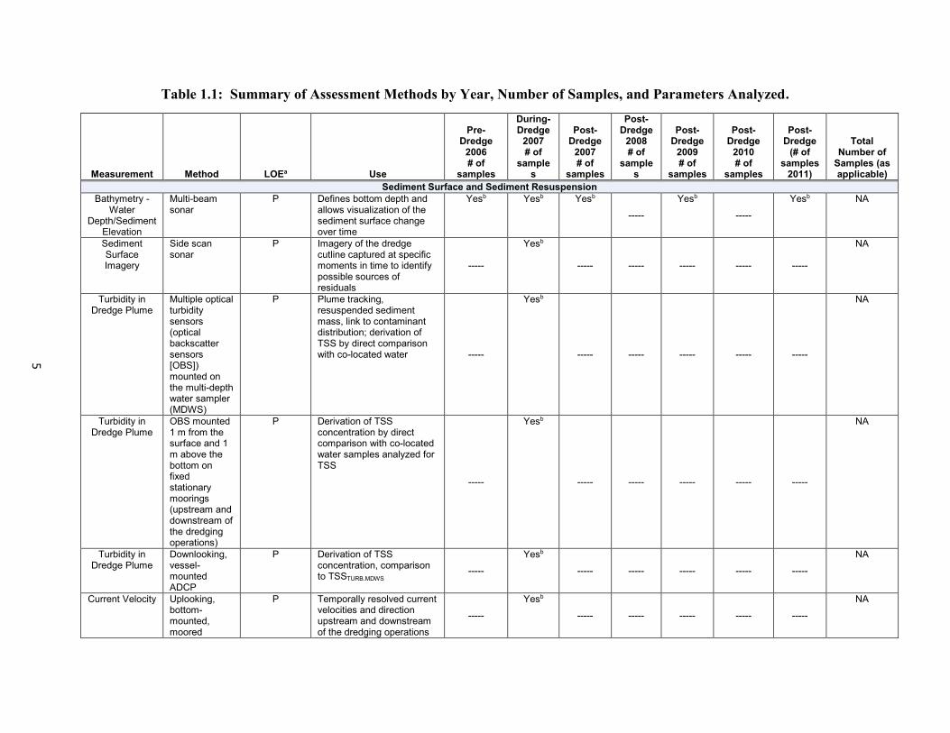
The research study involved samples collected, metrics measured, and methods applied through all stages of the remediaton project (pre-, during, and post-dredging). The characterizations of sediment, water column, and ecosystem quality were conducted from 2006 through 2011. Table 1.1 lists the measurements and the methods employed, their intended use, and the timeframe in which they were employed relative to dredging activities. Extensive pre-dredging characterization was completed in the summer of 2006. Subsequently, numerous sediment resuspension, sediment mapping (bathymetry and sidescan sonar), and ecosystem measurements were made during the dredging activities in 2007. Post-dredging characterization of sediment residuals and ecological indicators started in the fall and early winter of 2007. Post-dredging and long-term monitoring studies continued during 2008, 2009, 2010, 2011, and 2015. After dredging was completed, physical, chemical, and biological uptake measurements of dredging residuals 2F

1 were implemented using complementary techniques with an emphasis on measuring the quantity of COCs in the various matrices over time. Particular emphasis was given post-dredging to measuring the quantity and composition of the contaminants in dredge residuals in the sediment and the fraction of contaminated sediment removed by the dredging operation (i.e., estimating contaminated sediment removal efficiency).

1 Dredging residuals in the context of this report refer to contaminated sediment found at the post-dredging surface of the sediment profile, either within or adjacent to the dredging footprint.

5

Table 1.1: Summary of Assessment Methods by Year, Number of Samples, and Parameters Analyzed.

Measurement Method LOEa Use

Pre-Dredge

2006 # of

samples

During-Dredge

2007 # of

samples

Post-Dredge

2007 # of

samples

Post-Dredge

2008 # of

samples

Post- Dredge

2009 # of

samples

Post-Dredge

2010 # of

samples

Post-Dredge

(# of samples

2011)

Total Number of

Samples (as applicable)

Sediment Surface and Sediment Resuspension Bathymetry -

Water Depth/Sediment

Elevation

Multi-beam sonar

P Defines bottom depth and allows visualization of the sediment surface change over time

Yesb Yesb Yesb

-----

Yesb

-----

Yesb NA

Sediment Surface Imagery

Side scan sonar

P Imagery of the dredge cutline captured at specific moments in time to identify possible sources of residuals

-----

Yesb

----- ----- ----- ----- -----

NA

Turbidity in Dredge Plume

Multiple optical turbidity sensors (optical backscatter sensors [OBS]) mounted on the multi-depth water sampler (MDWS)

P Plume tracking, resuspended sediment mass, link to contaminant distribution; derivation of TSS by direct comparison with co-located water -----

Yesb

----- ----- ----- ----- -----

NA


OBS mounted 1 m from the surface and 1 m above the bottom on fixed stationary moorings (upstream and downstream of the dredging operations)

P Derivation of TSS concentration by direct comparison with co-located water samples analyzed for TSS

-----

Yesb

----- ----- ----- ----- -----

NA


Downlooking, vessel-mounted ADCP

P Derivation of TSS concentration, comparison to TSSTURB.MDWS -----

Yesb

----- ----- ----- ----- -----

NA

Current Velocity Uplooking, bottom-mounted, moored

P Temporally resolved current velocities and direction upstream and downstream of the dredging operations

-----

Yesb

----- ----- ----- ----- -----

NA

Table 1.1 (continued): Summary of Assessment Methods by Year, Number of Samples, and Parameters Analyzed.

6


Pre-Dredge

2006 # of

samples

During-Dredge

2007 # of

samples

Post-Dredge

2007 # of

samples

Post-Dredge

2008 # of

samples

Post- Dredge

2009 # of

samples

Post-Dredge

2010 # of

samples

Post-Dredge

(# of samples

2011)

Total Number of


acoustic Doppler current profiler (ADCP) (upstream and downstream of dredging operations)

Plume, Particle Volume and

Size Distribution

Laser in situ scattering and transmissometry (LISST) vertical profiles

P Derivation of volume concentration, bulk particle density for use in comparison to TSSTURB.MDWS -----

Yesb

----- ----- ----- ----- -----

NA

Total Suspended Solids (TSS)

Concentration

Water samples collected from the MDWS

P Plume tracking, resuspended sediment mass, link to contaminant distribution; Discrete water samples collected to determine TSS in the water column to correlate with vessel-mounted optical turbidity and acoustic backscatter (ABS) measurements

-----

148 TSSc

----- ----- ----- ----- -----

148

Total Suspended

Solids Concentration

Water samples collected at the stationary mooring locations

P Discrete water samples collected to determine TSS in the water column to correlate with moored optical turbidity and ABS measurements

-----

45 TSSc

----- ----- ----- ----- -----

45

Total PCBs in Water Column

MDWS discrete water samples – unfiltered

C Determine Total PCB mass concentrations and mass in dredge plume -----

148 PCBd

(CONe, HOMf),

GSg

----- ----- ----- ----- -----

148

Dissolved PCBs in Water Column

MDWS discrete water samples – filtered

C Determine dissolved PCB mass and concentration in dredge plume -----

155 PCBd

(CONe, HOMf)

----- ----- ----- ----- -----

155

Sediment Depth Profile ----- -----


7


Pre-Dredge

2006 # of

samples

During-Dredge

2007 # of

samples

Post-Dredge

2007 # of

samples

Post-Dredge

2008 # of

samples

Post- Dredge

2009 # of

samples

Post-Dredge

2010 # of

samples

Post-Dredge

(# of samples

2011)

Total Number of


Sediment Vibracoring and hydraulic piston coring

P Measure the physical characteristics of intact cores as a function of depth

328 GSg, WETh

from 30 stations

180 GSg, WETh

from 30 stations

No chemical analysis of 2009

core samples from 30 stations

160 GSg, WETh

from 28 stations

415 from 30 stations

Sediment Vibracoring and hydraulic piston coring

C Measure the chemical (PCB) characteristics of intact cores as a function of depth

369 PCBd

(CONe, HOMf,

PCB_IA), OTHER from 30 stations

58 PCBd

(CONe, HOMf), OTHER

180 PCBd

(CONe, HOMf), OTHER from 30 stations

No chemical analysis of 2009

core samples from 30 stations

165 PCBd

(CONe, HOMf), PAH,

OTHER from 28 stations

415 from 30 stations

Biological and Passive Samplers for Measuring Contaminant Uptake Macrobenthos Samplers and Co-located Sediment and Water

Macro-invertebrates –

from Macrobenthos

Stations

Macrobenthos samplers

B Measure chemical uptake (PCBs and PAHs) in macrobenthos during dredging operations

8 PCBd

(CONe, HOMf), PAHi,

OTHER

8 PCBd

(CONe, HOMf), PAHi,

OTHER

-----

8 PCBd

(CONe, HOMf), PAHi,

OTHER

8 PCBd

(CONe, HOMf), PAHi,

OTHER

10 PCBd

(CONe, HOMf), PAHi,

OTHER

12 PCBd

(CONe, HOMf), PAHi,

OTHER

54

Sediment/ Surface

Sediment from Macrobenthos

Stations

Sediment push core sampler – top 0.15 m

C Measure chemistry (PCBs and PAHs) in surface sediments co-located with Macrobenthos stations during dredging operations; compare spatial and temporal trends

4 4

-----

8 12 10 5 51 PCBd

(CONe, HOMf)

GSg, TOCj

GSg, TOCj, PCBd

(CONe, HOMf), PAHi

GSg, TOCj, PCBd

(CONe, HOMf), PAHi

GSg, TOCj, PCBd

(CONe, HOMf), PAHi

GSg, TOCj, PCBd

(CONe, HOMf), PAHi

8 PCBd

(CONe, HOMf), PAHi

Water – from Macrobenthos

Stations

Water grab sampler

C Measure chemistry (PCBs and PAHs) in water samples co-located with Macrobenthos stations during dredging operations; compare spatial and temporal trends

4 8

-----

8 12 10

-----

42 PCBd

(Integration)

PCBd (CONe),

PAHi

PCBd (CONe),

PAHi

PCBd (CONe),

PAHi

PCBd (CONe),

PAHi


8


Pre-Dredge

2006 # of

samples

During-Dredge

2007 # of

samples

Post-Dredge

2007 # of

samples

Post-Dredge

2008 # of

samples

Post- Dredge

2009 # of

samples

Post-Dredge

2010 # of

samples

Post-Dredge

(# of samples

2011)

Total Number of


Semipermeable Membrane Device/Solid Phase Micro-extraction (SPMD/SPMEs) and Co-located Sediment and Water

Sediment Semipermeable

Membrane Device (SPMD)

SPMD deployed on sediment surface

C Measure PCB uptake in samplers positioned on the sediment surface

25

----- -----

26

----- -----

13 64 PCBd

(CONe, HOMf)

PCBd (CONe, HOMf)

PCBd (CONe, HOMf)

Water Semipermeable

Membrane Device (SPMD)

SPMD deployed in water column

C Measure PCB uptake from the water column

12

----- -----

10

----- -----

13 35 PCBd

(CONe, HOMf)

PCBd (CONe, HOMf)

PCBd (CONe, HOMf)

Sediment Solid Phase Micro-

extraction (SPME)

SPMD deployed on sediment surface

C Measure PCB uptake in samplers positioned on the sediment surface

14

----- -----

15

----- ----- -----

29 PCBd

(CONe, HOMf)

PCBd (CONe, HOMf)

Water Solid Phase Micro-

extraction (SPME)

SPMD deployed in water column

C Measure PCB uptake from the water column

6

----- -----

10

----- ----- -----

16 PCBd

(CONe, HOMf)

PCBd (CONe, HOMf)

Sediment/ Surface

Sediment from SPMD/SPME

Stations

Sediment push core sampler – top 0.15 m

C Measure PCBs in surface sediments co-located with SPMD/SPME stations during dredging operations; compare spatial and temporal trends

10

----- -----

11

----- -----

11 32 PCBd

(CONe, HOMf) GSg,

TOCj

PCBd (CONe, HOMf) GSg, TOCj

PCBd (CONe, HOMf) GSg, TOCj

Water – from SPMD/SPME

Stations

Water grab sampler

C Measure PCBs in water samples co-located with SPMD/SPME stations during dredging operations; compare spatial and temporal trends

10

----- -----

12

----- -----

12 33 PCBd

(Integration)

PCBd (CONe, HOMf)

PCBd (CONe, HOMf)

Fish and Bivalves

Indigenous Fish (Brown

bullhead [BB], channel catfish,

shiners)

Electroshocking

C Measure PCB uptake in fish during dredging operations

10 BBk 9 BBk 10 BBk 10 BBk 20 BBk 40 BBk 150 PCBd

(CONe, HOMf), PAHi,

OTHER;

PCBd (CONe, HOMf), PAHi,

OTHER


OTHER


OTHER


OTHER


OTHER 45

Channel Catfish

-----

6 Shiner

PCBd (HOMf), OTHER

PCBd (CONe, HOMf),


9


Pre-Dredge

2006 # of

samples

During-Dredge

2007 # of

samples

Post-Dredge

2007 # of

samples

Post-Dredge

2008 # of

samples

Post- Dredge

2009 # of

samples

Post-Dredge

2010 # of

samples

Post-Dredge

(# of samples

2011)

Total Number of


PAHi, OTHER

Caged Bivalves Caged bivalve deployment

C Measure PCB uptake in bivalves (Corbicula fluminea) during dredging operations

10 stations ----- ----- ----- ----- ----- -----

0 No survival

Caged Worms Caged worm deployment

C Measure PCB uptake in worms (Lumbriculus variegatus) during dredging operations

10 stations No survival ----- ----- ----- ----- ----- -----

0

Water Column for Overall Site Characterization

Post-Dredge Water Column

Samples

Grab samples for PCB and PAH analyses

C Whole water sampled at the centerline/midpoint of each transect at mid-water depth to measure PCBs and PAHs in the water column prior to and following dredging

14 PCBd

(HOMf) -----

13 PCBd

(CONe, HOMf), PAHi

11 PCBd

(CONe, HOMf), PAHi

15 PCBd

(CONe, HOMf), PAHi

----- -----

53

NA = Not applicable iPAH = Polycyclic aromatic hydrocarbon aP = physical; B = biological; C = chemical jTOC = total organic carbon bYes = electronic data sampling effort/survey was conducted during this period kBB = brown bullhead cTSS = Total suspended solids dPCB = Polychlorinated biphenyl eCON = PCB congeners (analysis) fHOM = PCB homolog (analysis) gGS = grain size (particle size distribution) hWET = gravimetric wet weight of sample

10

The results for the dredging residuals studies were summarized in a comprehensive interpretive report titled “Field Study on Environmental Dredging Residuals: Ashtabula River, Volume I. Final Report” (U.S. EPA, 2010).

The biological characterization methods developed and demonstrated were designed to evaluate ecosystem recovery following remediation of contaminated sediments. The biological studies were initiated prior to dredging in 2006 and continued through the period of dredging operations and extended post-dredging through 2011 (4 years of annual post dredging assessment). Macrobenthos contaminant concentrations was sampled using Hester-Dendy (H-D) artificial substrate samplers deployed to collect macrobenthos. Additional biological evaluations were conducted immediately post-dredging and included assessing native brown bullhead catfish, and deployment of bivalves (Corbicula fluminea) and oligachaetes (Lumbriculus variegatus) to measure chemical uptake; however, limited survival during these deployments curtailed further study. Additionally, the potential uptake of the contaminants into organisms was measured with passive samplers known as semipermeable membrane devices (SPMDs) and solid phase micro-extraction (SPME). These samplers were placed in contact with surface sediment and in the water column. The results from these biological and ecosystem investigations were summarized in a comprehensive interpretive report entitled “Data Report on Ecosystem Monitoring for the Ashtabula River Environmental Dredging Project” (U.S. EPA, 2011b).

To characterize the potential for contaminant mass redistribution during dredging, a water sampling program was implemented during dredging operations. This characterized the extent of the suspended solids plume generated by dredging activities, including estimating the volume and concentrations of suspended sediments over time, estimating the concentrations of PCB and PCB mass associated with the suspended sediments over time, and estimating the mass of the resuspended sediment and associated PCBs in the post-dredge residuals.

This report presents a summary of the research conducted by U.S. EPA ORD during the Ashtabula River Environmental Dredging Project, including brief summaries of the previously published U.S. EPA reports (USEPA 2010 and 2011). Data from all monitoring years (2006 to 2011) were integrated to address the ORD research program goals.

Results from this ORD study and of studies performed by U.S. EPA’s partners will also be used to address GLNPO’s project goal to conduct a remedy effectiveness assessment and to support beneficial use impairment (BUI) removal. BUI removal and data to support delisting the AOC will be addressed GLNPO at a later date.

Section 2.0 of this report summarizes the experimental approach and provides summary level details of the methods used to conduct the program. Section 3 presents the results utilizing the methods described in Table 1.1. Section 4 provides an assessment of the methods applied during the research project and their utility in characterizing environmental conditions relative to the remediation activities. Section 5 considers the uncertainties relative to the project goals and overall conclusions derived from the study. Section 6 provides references cited in this report.

11

2.0 EXPERIMENTAL APPROACH Pre-, during-, and post-dredging field studies were conducted from 2006 to 2011. These studies adhered to U.S. EPA-approved QAPPs (U.S. EPA, 2006; 2007; 2011a). The QAPPs described the projects’ purposes and goals, field collection methods, analytical methods, and quality assurance/quality control (QA/QC) requirements for each year. Field sampling activities carried out before, during, and after dredging consisted of a multiple LOEs approach using physical, chemical, and biological measurements to understand the transport and fate of the COCs resulting from environmental dredging and the impacts to ecosystem endpoints. The ORD research program evaluated a range of physical, chemical, and biological sampling devices and measurements for characterizing residuals resulting from contaminated sediment dredging. These research studies were designed to reduce the uncertainty surrounding the use of these methods for evaluating future remediation and recovery monitoring of contaminated sediment sites. ORD specifically focused on fate and transport of COCs using bathymetry, plume tracking (transport), and physical and chemical characterization of the sediment prior to remediation and in post-dredge residuals. Biological and passive samplers were used for estimating the uptake (fate) of organic chemicals in biota. The research further examined the use of chemical characteristics of the PCBs (i.e., congeners, homologs) and changes between pre- and post-remediation for measuring long-term recovery following environmental dredging. The study further compared and contrasted the chemical composition in organism and passive samplers to the original sediments and post-remediation residuals to support the assessment method evaluation. Co-located passive samplers, sediment, and water data enabled comparison of the passive sampler data for potential use in the remedy effectiveness assessment. The following describes the data collection approach for each of the methods described in Table 1.1. 2.1 Sediment Mapping

2.1.1 Bathymetry

The bathymetry of the study area was mapped during several surveys by multi-beam sonar/side scan sonar (MBS/SSS). The sonar system was deployed by boat to survey the river’s sediment surface prior to dredging (2006), following dredging operations in 2007, and again in 2009 and 2011. Section 2.3.2 of the Dredge Residuals Report (U.S. EPA, 2010) details the MBS/SSS bathymetric survey methods utilized in 2007 and 2009, which was conducted by ORD, Battelle, and Integral Consulting, Inc. (ICI). Bathymetry was measured in 2011 by the U.S. Army Corps of Engineers (USACE) Buffalo District.

12

The sediment surface was also mapped daily to the extent possible during dredging. The bathymetric variability and dredge cut slump progression was documented and representations of the modified riverbed developed post-dredging. Survey data quality was assured with daily verification of proper system operation and verification of the accuracy (satellite corrected) of the global positioning system (GPS) position, and vessel heading data. MBS calibrations and soundings were verified daily with sound velocity casts in the water column and bar checks 3F

2 for the sonar depth offsets. The vertical survey control was verified by comparing the water level logger real-time output with manual elevation measurements at the location of the logger.

2.1.2 Sidescan Sonar

SSS was used to qualitatively identify materials on the sediment surface prior, during, and post-dredging. SSS surveys were used to characterize the extent of debris prior to dredging. Debris is suspected to result in higher dredge residuals due to inefficiency and disruption of the bedded sediment during dredging. In addition, SSS during dredging over short time intervals allowed for the identification of cut failures due to sediment sloughing. 2.2 Plume Tracking

In May, June, and July of 2007, Battelle and ICI with EPA ORD collected water quality data to evaluate the character and extent of the suspended solids plume generated due to Ashtabula River dredging activities, including estimating the volume and concentrations of suspended sediments over time, estimating the PCB concentrations and mass associated with the suspended sediments over time, and estimating the mass of the resuspended sediment and associated PCBs contributing to the residuals after dredging. ICI deployed submerged water quality moorings with mounted optical turbidity sensors and acoustic Doppler current profiler (ADCP) platforms at distinct upstream and downstream locations to measure turbidity (nephelometric turbidity units; NTU), current velocity, and acoustic backscatter (ABS) at stationary locations. An additional downward-looking ADCP was mounted from a vessel to measure current velocity and ABS at cross-channel spatially varying locations in the river, upstream and downstream of the dredging operation. Battelle’s multi-depth water sampler (MDWS) was installed on the same vessel as the ADCP and was used to collect water samples coinciding with plume locations identified from real-time turbidity data. Optical backscatter system (OBS) sensors were mounted at each of the four sampling depths of the MDWS to provide continuous, multi-depth turbidity measurements. The water samples and optical turbidity were collected simultaneously with ADCP measurements to allow for correlation between sensor turbidity measurements and TSS measurements. Periodically, discrete water samples were collected and analyzed for total suspended solids (TSS) and PCB concentrations.

2 Bar checks are made using a flat object held at predetermined distances beneath the MBS transducers to ensure proper depths are recorded.

13

Turbidity measurements collected with the MDWS were recorded for bank-to-bank river (cross-river) transects both upstream and downstream of the dredging activities. The data from the MDWS and ADCP were used to develop multi-dimensional maps of sediment plumes in the remediation area. The MDWS and ADCP were first deployed on June 1-9, 2007 (Figure 2-1) and produced turbidity data for 260 transects over 9 days. A second survey conducted between July 23 and 25, 2007 produced depth specific turbidity data for 70 transects over 3 days (Figure 2-2). Particle size distributions (PSDs) of the suspended sediment were determined using a laser in situ scattering and transmissometry (LISST) sensor that was vertically profiled at approximately mid-channel during ADCP and MDWS vessel-based sampling. A LISST-100X, type B was deployed in the center of channel cross-sections for a percentage of transects measured with the ADCP and MDWS (Sea Engineering, Inc. [SEI], 2007; Appendix A to this report). The type B sensor measured the size distribution for particles between 1.4 and 231.0 µm in diameter using laser diffraction technology. Discrete water samples were also collected for laboratory measured particle size determination to correspond with the LISST measurements. Details of the field collection activities and data analyses are provided in the full SEI report provided in Appendix A.

The exact transect spacing was determined in the field and selected to spatially (horizontally and vertically) characterize the sediment plume associated with dredging operations. Similarly, the frequency of surveys was subject to change after initial dredge plume assessment. Surveys of this type occurred several times per day.

The MDWS’s multi-depth water collection capability enabled simultaneous collection of water samples at selected depth intervals. The suspended solids fraction of the water sample was analyzed for particulate-associated PCBs. The aqueous fraction was analyzed for dissolved PCBs. Whole water split samples were analyzed for turbidity, TSS, PSD, and total organic carbon (TOC).

In all, a total of 45 whole water samples were collected and analyzed for turbidity, TSS, and PSD, and a total of 148 samples were filtered for total and dissolved PCB analyses as described in Section 2.9.2.

The ADCP was used to measure surface water velocities for future application of sediment transport models to estimate particle and contaminant flux in the water column. The boat-mounted ADCP was mounted to the boat hull in a downward-looking position from the water surface. Surveys with the ADCP occurred concurrently with collection of water samples using the boat-mounted MDWS to determine the water column flux (mass transport rate) of sediments and contaminants and quantify the amount of suspended material in the water column.

14

Note: Code for dredge location = month/day

Figure 2-1. June 2007 Survey Whole Water Sample Collection Locations and Dredge Positions of the Michael B.

Survey

Date

Water Sample

Collection

Locations

AR-024

AR-025

3-Jun-07 AR-047

AR-048

AR-053

AR-054

AR-055

AR-056

AR-097

AR-098

AR-099

AR-105

AR-116

AR-117

AR-118

AR-119

AR-121

AR-186

AR-202

AR-205

AR-207

AR-208

AR-209

AR-210

AR-233

AR-254

1-Jun-07

4-Jun-07

5-Jun-07

6-Jun-07

8-Jun-07

9-Jun-07

15

Note: Code for dredge location: PB (Palm Beach) or MB (Michael B) and month/day

Figure 2-2. July 2007 Survey Whole Water Sample Locations and Dredge Positions of the Michael B. (“MB”) and the Palm Beach (“PB”).

Survey

Date

Water Sample

Collection

Locations

AR-306

AR-309

AR-311

AR-312

AR-331

AR-333

AR-334

AR-335

AR-336

AR-337

AR-338

23-Jul-07

16

When possible, three transects were run while: 1) the dredge was operating at a single location, 2) turbidity was visually present, and 3) river flow was in one direction. One transect was performed close to the dredge, one mid-plume, and one far-plume. Due to dredge operations, vessel traffic, and river flow conditions, it was not always possible to collect data along the three target transects relatively coincidental. The following are descriptions of near-dredge, mid-plume, and far-plume.

Near-dredge refers to a transect located as close as safely possible to the dredge. This distance was estimated as typically <15 m.

Mid-plume was in a location approximately midway between the dredge and where evidence of the plume was not distinguishable based on visual observations. This distance was typically between 30 and 60 m.

Far-plume was at the edge of the visible plume. This distance was typically between 60 and 120 m.

2.3 Sediment Sediment was collected in support of a number of different field studies including:

Deep sediment cores collected pre- (2006) and post- (2007, 2009, and 2011) dredging to determine the historical physical and chemical profiles and to estimate dredging residuals (U.S. EPA, 2010).

Surface sediment cores (0 to 10 cm) were collected at positions co-located with both passive samplers (SPMDs, SPMEs) and with the macrobenthos samplers (H-Ds) to allow correlation of passive samplers and macrobenthos tissue concentrations with sediment from the same locations over time and space.

The following describes sediment collections. 2.3.1 Sediment Cores

A total of 30 sediment cores were collected from the study area prior to dredging in 2006, again upon completion of dredging in 2007, and in long-term monitoring in 2009 and 2011 (Figure 2-3). These 30 stations served as repeated monitoring positions for evaluating dredge residuals. The name and geoposition are provided in U.S. EPA (2010). The following describes the sample collection activities and the core processing procedures and strategy for each event.

2.3.1.1 Sediment Core Collection

Pre-dredge 2006 Sediment Cores. Sediment cores collected prior to dredging, where sediment thickness was at its maximum extent, were collected using a vibracoring method. All pre-dredge sediment cores were sampled to the point of refusal. Consistent with the original plan, it was presumed that the area consisting of transects T181 to T177 would be dredged to a depth confined by the bedrock layer, while dredging would continue only to 6 m below the IGLD85 (International Great Lakes Datum of 1985) in the area containing transects T177 to T170, leaving a layer of soft sediment above bedrock. As such, collection of sediment cores to refusal

17

ensured that the pre-dredge sediment cores would be as deep as or deeper than the target cut line. In this way, a total of 16 sediment cores were collected in the area that was planned for dredging to bedrock and 14 sediment cores were collected in the soft sediment area. When coupled with chemical analysis, this allowed for a full PCB vertical profile of the sediment above and below the target cut line.

Pre-dredging sediment cores were collected from a vessel with a pneumatic vibracore sampler. The vibracore consisted of a vibratory head connected to a 10-cm outside diameter steel or stainless steel tubing with a stainless steel core cutter and catcher. Core tubing was lined with a pre-cleaned polyethylene tube of approximately 6 to 8 mil thickness. Cores were collected until refusal from native bedrock or to approximately 1.0 m below target dredge depth. Post-dredge 2007 Cores. The post-dredge sediment cores were collected in November 2007 following completion of dredging in June 2007; cores were collected using a hand push core sampler or a hydraulically-driven piston core device. Samples were collected to a maximum depth of approximately 1.5 m in some areas, with the intention to capture the post-dredge surface sediment and native (un-dredged) sediment below. The cores were delivered intact to the laboratory for processing and analysis.

Figure 2-3. Sediment Core Sample Locations in the Ashtabula River Residual Study Area for Pre- (2006) and Post- (2007, 2009, and 2011) Dredging, respectively.

LTM 2009 Cores. The 2009 cores were collected from 30 stations using either a vibracore or, where leaf deposits prevented penetration of the vibracore unit, a hand-driven piston core device.

18

A core was collected at each station and a duplicate core at five of the 30 stations (T170A, T173A, T176A, T179A, and T181C). The cores were processed and physically characterized in the fall of 2011, but not analyzed for PCBs as a cost cutting measure. Core samples collected in 2011 were used to determine additional post-dredge PCB profiles.

LTM 2011 Cores. In 2011, 35 sediment cores were collected (28 sample locations and seven duplicate core samples) using a pneumatically-driven piston core. Two stations (T177A and T179A) were not sampled because the surface elevation was determined to be below the bottom depth of the previously collected core (2009) indicating potential scouring of the location.

2.3.1.2 Core Processing

Following penetration and removal, the core enclosed in the liner was removed from the core tube, examined for integrity and volume, labeled and stored upright until processing. The 2006 cores were cut into manageable lengths for shipment and “reconstructed” in the laboratory for further processing as well as physical and chemical characterization. Cores collected in 2007, 2009, and 2011 were of shorter length and not cut in the field for shipment. They were processed entirely in the laboratory. Cores collected in 2009 were held in a refrigerator and processed in parallel with the 2011 cores. Cores were partitioned into segments of various length depending on physical characteristics, and each segment was photographed and identified with a placard containing the project name, date, sample station identification (ID), and a measuring tape showing the length of the core. Cores were described following American Society for Testing and Materials (ASTM) Procedure D2488-93 (ASTM, 1993). Features such as sediment type (silt, clay, sand, etc.), color, consistency, sedimentary structure, and odor were documented. Core material was extracted from each polyvinyl chloride sleeve for analysis by splitting the sleeve lengthwise and removing sediment from the internal portion of the core to avoid sediments that may have adhered to the sidewalls of the sleeve during coring. Sediment samples were transferred to a pre-cleaned stainless steel bowl using a cleaned stainless steel spoon. The sediment was homogenized to a uniform color and consistency and then distributed into the appropriate pre-labeled, certified-clean containers (U.S. EPA, 2007). 2006 Core Processing. Each sediment core collected in 2006 was cut with a portable hand or battery-powered saw into intervals of 30 cm or less in the field and submitted to the laboratory for processing and analysis. Sediment core lengths were “reconstructed” on the laboratory bench top, and photographs of each core were taken and recorded. The length of each sediment segment was determined upon physical observation of the core with greater delineation focused in the range of the target cut line or dredge depth. The segments were based on sediment characteristics and previously collected cores/segments for comparison between sampling years. Each core segment was processed further by mixing in a laboratory blender for approximately 5 minutes before analysis. Core segments were analyzed for PCB congeners, TOC, PSD, and bulk density.

19

2007 Core Processing. Post-dredge sediment cores were processed in the same manner previously described. The sediment segment thickness decreased in the range of the target cut line, and the frequency of segments in this depth range increased. The post-dredge bathymetric survey, as well as visual observations of note and consideration of the target cut line elevation, played a major role in the decision process as to where the post-dredge sediment cores would be sectioned. Sediment cores collected during the pre- and post-dredge sampling events from each sampling station were aligned vertically using elevation data to compare pre- and post-core segments and determine their relationship to the dredge cut line. Several parameters were used independently and in combination to verify alignment for pre- and post-dredge core comparisons. These included water depth information, core lengths, refusal depth, and pre- and post-dredge bathymetric survey data. Post-dredge core sections were processed and analyzed for the same parameters as the pre-dredge core sections. 2009 and 2011 Core Processing. In the fall of 2011, the 2009 and 2011 cores were processed and analyzed in a similar manner as noted above for the 2006 and 2007 cores. The 2009 and 2011 cores were segmented based on the 2007 segmentation plan and were virtually aligned with the 2007 core data using elevation data. For the 2009 and 2011 cores, material was processed in 15-cm segments from the water surface interface down and from the 2007 surface elevation up leaving an odd length core segment in the middle. Any material below the 2007 bottom elevation was segmented in 15-cm intervals. Segment sizes from the section of the core that overlapped with the 2007 core ranged from 1.5 to 7.5 cm. For cost efficiency and to reduce the number of samples for analysis, the 2011 subsamples were composited following a compositing scheme prepared by Battelle and accepted by U.S. EPA. When the core material appeared to be new depositional material (based on elevation data), the top 15 cm were collected first and then advancing 30-cm intervals were collected until the 2007 surface elevation was met. The subsamples taken from the subsection of the core that corresponded with the 2007 surface elevation were composited based on 2007 total PCB analytical data (<1 part per million [ppm], 1 to 10 ppm, 10 to 50 ppm, and >50 ppm). The composited sample intervals ranged from 3 to 30 cm. Any material collected below the bottom depth of the 2007 core was not analyzed. Water samples were collected prior to deployment and retrieval to avoid sampling particulate material entering the water column during equipment placement. Water was collected with a Van Dorn or Niskin type sampler. Care was taken to prevent sampler contact with the bottom to avoid disturbing bottom sediments. Sample jars were filled with site water, placed on ice, and distributed to the analytical laboratories for PCB, PAH, TOC, and TSS analysis (U.S. EPA, 2007). 2.4 Passive Samplers Two types of passive sampling devices were deployed for 28 days to mimic biological uptake of COCs from either the water column or sediment surface. These consisted of SPMDs and SMPEs. The SPMDs were deployed on the sediment surface (Figure 2-4) and in the water

20

column (Figure 2-5) for 28 days at 10 to 11 stations (depending on year) in 2006, 2008, and 2011. SPMEs were only deployed in conjunction with the water column and sediment SPMDs in 2006 and 2008. The following subsections describe the devices themselves and the deployment methodologies. 2.4.1 Passive Samplers: Semipermeable Membrane Device

The SPMDs used for this program were composed of flat, low-density polyethylene tubing containing a thin film of a pure, high-molecular-weight lipid (triolein). The triolein oil was spiked with a known amount of a surrogate or performance reference compound (PRC). The PRC was used to estimate the sampled water volume using a formula developed by the U.S. Geological Survey (USGS) that takes into account partition coefficients and the concentration of remaining PRC at the time of retrieval and is discussed further in Section 3.6. PRC was spiked into the triolein oil batch at a mass of 50 ng of each PCB congener per SPMD sample. The PRC matrix consisted of the following mixture of PCBs in hexane each year:

2006: PCB 38, PCB 50

2008: PCB 29, PCB 38, PCB 150, PCB 166

2011: PCB 8, PCB 186 These PCB congeners were selected as the field PRCs because they were all good indicators of target PCB behavior and were not detected in prior characterization of the site. Over the course of the project, different analytes were used for this PRC matrix to minimize co-elutions with the target analytes. SPMDs were deployed on the surficial sediments using a device called an “SPMD rack” (Figure 2-6) and in the water column using a device called a “spider carrier” (Figures 2-7 and 2-8) (Schubauer-Berigan et al., 2012). The SPMD racks were designed and provided by U.S. EPA; the spider carriers and SPMDs were provided by Environmental Sampling Technologies, Inc. (EST) of St. Joseph, MO.

Table 2.1 identifies the sampling locations where the sediment and water column SPMDs were deployed. SPMD racks were deployed at Stations 1 through 21 for the 2006 and 2008 sampling events. Water column SPMD canisters were deployed at 10 of the 21 stations. In 2011, SPMD racks were deployed on the sediment surface and SPMD canisters were deployed in the water column at 10 of the 21 locations from 2006 and 2008.

21

Figure 2-4. Sediment SPMD Deployment Locations.

22

Figure 2-5. Water Column SPMD Deployment Locations.

23

Figure 2-6. Typical SPMD Rack Design for Deployment of SPMDs on the Surficial Sediment.

Figure 2-7. Top View and Angle View of the SPMD Spider Carrier (EST, St. Joseph, MO).

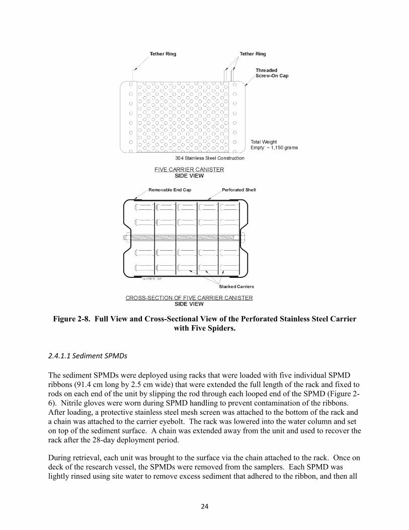
24

Figure 2-8. Full View and Cross-Sectional View of the Perforated Stainless Steel Carrier with Five Spiders.

2.4.1.1 Sediment SPMDs

The sediment SPMDs were deployed using racks that were loaded with five individual SPMD ribbons (91.4 cm long by 2.5 cm wide) that were extended the full length of the rack and fixed to rods on each end of the unit by slipping the rod through each looped end of the SPMD (Figure 2-6). Nitrile gloves were worn during SPMD handling to prevent contamination of the ribbons. After loading, a protective stainless steel mesh screen was attached to the bottom of the rack and a chain was attached to the carrier eyebolt. The rack was lowered into the water column and set on top of the sediment surface. A chain was extended away from the unit and used to recover the rack after the 28-day deployment period. During retrieval, each unit was brought to the surface via the chain attached to the rack. Once on deck of the research vessel, the SPMDs were removed from the samplers. Each SPMD was lightly rinsed using site water to remove excess sediment that adhered to the ribbon, and then all

25

five ribbons were transferred into a common hexane-rinsed can for shipment to EST for processing and dialysis (extraction).

Table 2.1: Summary of SPMD Deployment Years and Locations.

Station ID 2006 2008 2011

SPMD-S

SPMD-W SS W(a) SPMD

-S SPMD

-W SS W(b) SPMD-

S SPMD

-W SS W(a)

PS-01 * * - - * PS-02 - - - - - - - - - - PS-03 * * * PS-04 ** * PS-05 * PS-06 * - - - - - - - - - - PS-07 - - - - - - - - - - PS-08 PS-09 - - - - - - - - - - PS-10 - - - - - - - - - - PS-11 - - - - - - - - - - PS-12 -

(c) PS-13 - - - - - - - - - - PS-14 - - - - - - - - - - PS-15 PS-16 - - - - - - - - - - PS-17 - - - - - - - - - - PS-18 - - - - - - - - - - PS-19 - - - - - - - - - - PS-20 - - - - - - - - - - PS-21 - - - - - - - - - - PS-22 - PS-23 - * * PS-24 - * * PS-25 - - SPMD-S: Sediment SPMD SPMD-W: Water SPMD SS: Surface Sediment W: Surface Water “-“ No sample deployed at this station. “*” Duplicate sediment SPMD racks deployed at this station. Average of duplicates used in data evaluation. (a) 2006 and 2001 water samples collected during deployment of SPMD samplers only. (b) 2008 water samples collected during deployment and retrieval of SPMD samplers. (c) Water samples were collected during deployment of SPMD only at Station 12. No water column SPMD or water samples were collected during retrieval at Station 12 in 2008.

2.4.1.2 Water Column SPMDs

SPMDs were deployed in the water column using large canisters that were supplied by EST. Water column SPMDs were shipped to the field mounted on the spider carrier (see Figure 2-7). Each spider carrier contained one full-length of SPMD ribbon (90 cm long by 2.5 cm wide) that

26

was “woven” through spindles on the spider carrier to maximize surface area for exposure and uptake. For each water column deployment, a total of five spider carriers were stacked onto a central post within a perforated stainless steel carrier canister (Figure 2-8). The canister was secured with a screw-top lid. The canister’s holes allowed for ample movement and circulation of water through the device once it was deployed into the water column. Water column SPMD deployments were attached to the chain of the SPMD rack, with the rack serving to anchor the water deployment in place. Each water column canister was fitted with a subsurface buoy so that the canister was allowed to float approximately 1 m above the sediment surface. Water column deployments were the first to be retrieved from a given station to minimize impacts from disturbed sediments. Each canister was brought to the surface, and the top of the canister was removed. Each of the five spider carriers was removed from the canister and transferred into a hexane-rinsed can with the SPMD left in place on the carrier and shipped to EST for extraction. The spider carriers from a station were combined as a single sample. 2.4.1.3 Surface Sediments

Surface sediment samples were collected (top 10 cm) at locations corresponding to deployments for passive samplers (SPMD/SPME). For most years, surface sediments were collected from these same locations when the equipment was retrieved. Table 2.1 identifies the sampling locations where surface sediment was collected in association with SPMDs. A stainless steel ponar sampler was used to collect surface sediment samples in 2006 through 2010. In 2001, the Undisturbed Surface Sediment (USS) sampler, a unique sampler developed by U.S. EPA/NERL’s Environmental Sciences Division, was used to collect surface sediment samples. At least one sample from each location was photographed in the grab or core sampler after placing a placard containing the project name, date, and sample station ID on the sampler. The top 10 cm of each grab sample or core was transferred to sample containers by transferring a portion of sediment with pre-cleaned stainless steel spoons. Sediment that contacted the walls of the grab sampler or core barrel was not included in the sample. Each sample’s general characteristics (e.g., sediment type [silt, clay, sand, etc.], color, consistency, sedimentary structure, and odor) were recorded on a Sediment Characterization form (Appendix D). Sediment from each location was field homogenized to a uniform color and consistency by hand using stainless steel utensils. Homogenized samples were placed on ice and shipped to pre-approved analytical laboratories for PCB, PAH, PSD, and TOC analysis. 2.4.1.4 Water Column Samples

Whole water samples were collected at passive sampler (SPMDs, SPMEs) stations to correlate water column data with passive sampler results. Table 2.1 identifies the sampling locations where water column samples were collected in association with SPMDs. Water samples were collected approximately 15 to 30 cm above the sediment-water interface. This depth was deemed sufficient to collect water samples as close to the sediment surface as possible while taking caution not to disturb the bottom sediments. Water samples were collected with a Niskin sampler.

27

2.4.2 Passive Samplers: Solid Phase Micro-Extraction

In 2006, SPME devices consisted of a fiber optic material with an external non-polar coating which was used to accumulate non-polar organic compounds, such as PCBs, at a known rate based on equilibrium partitioning. Commercially available SPME fibers (Supelco, Part# 57341-U) were purchased and affixed inside a 6-in. stainless steel mesh Geoprobe™ well screen that was modified with a removable screw cap. Each mesh “container” was fixed with a thin gauge steel wire to the outside of either an SPMD water column deployment or the inside of the protective screening of the SPMD rack. At retrieval, it was found that the wire tie used to fix the SPMEs to the SPMD deployments corroded considerably over the 28-day deployment period and most of the SPMEs that were attached to the outside of the water column SPMD carriers were lost, as well as most of those that were attached to the SPMD racks. In 2008, an alternative deployment approach and SPME material, similar to that described in Burgess et al. (2015), was used. SPMEs were derived from a fiber optic material (Fiberguide, Inc.) and cut to length in the laboratory. The fibers consisted of a polydimethylsiloxane (PDMS) coating. This material was demonstrated to be equivalent to commercially available SPME devices for a wide range of hydrophobic analytes. For field sampling, the disposable fibers provided a significant reduction in cost over the commercially available SPME fibers. The SPME fiber was cut into 3-cm long pieces. The specifications of each fiber piece were as follows:

Fiber piece length: 3 cm;

PDMS coating thickness: 10 μm;

Diameter of silica core: 210 μm;

Diameter of fiber piece (PDMS coating + silica core): 230 μm

Volume of PDMS coating: 0.207 μL;

Density of PDMS coating: 1.05 μg/μL;

Weight of PDMS coating: 0.22 μg. These SPMEs were transferred into a stainless steel mesh pouch (Burgess et al., 2015). Each pouch was pre-cleaned and wrapped in aluminum foil for shipment to the site. The stainless steel pouch was fixed inside the water column SPMD carriers and inside the mesh screen of the SPMD racks. For each location, two SPME samplers were deployed. The duplicate SPME sampler served as a backup sample in the event the primary sample was compromised during the sampling. The SPMEs were retrieved after the 28-day deployment period. All SPMEs including the duplicates were retrieved from each location and shipped to the laboratory for processing, extraction, and analysis. Table 2.2 summarizes the deployment locations for 2006 and 2008 and the collection locations for co-located surface sediment and water samples.

28

Table 2.2: Summary of SPME Deployment Years and Locations.

Station ID

2006 2008

SMPE-S SPME-W SS W(a) SPME-S SPME-W SS W(b)

PS-01 * - PS-03 * * PS-04 * * PS-05 * * PS-06 - - - - - - PS-07 - - - - - - PS-08 PS-10 - - - - - - PS-11 - - - - - - PS-12

(c)

PS-15 PS-22 - - PS-23 - - PS-24 - - PS-25 - - -

SPME-S: Sediment SPME SPME-W: Water SPME SS: Surface Sediment W: Surface Water “-“ No sample deployed at this station. “*” Duplicate sediment SPME racks deployed at this station. Average of duplicates used in data evaluation. (a) 2006 and 2001 water samples collected during deployment of SPMD samplers only. (b) 2008 water samples collected during deployment and retrieval of SPMD samplers. (c) Water samples were collected during deployment of SPMD only at Station 12. No water column SPMD or water samples were collected during retrieval at Station 12 in 2008.

2.5 Macrobenthos Sample Collection Macrobenthos artificial substrate samplers were used to collect macrobenthos tissue for chemical analysis. Each deployment system consisted of units called Hester-Dendy (H-D) multi-plate samplers (Figure 2-9). Each sampler consisted of eight square pieces of tempered hardboard plate set up with increasing top to bottom spacing intervals (Figure 2-9); see Lazorcheck et al. (2015) for more details. The entire sampler was held together with an eyebolt and wing nut assembly. The plates (7.6 cm × 7.6 cm) and spacers (2.5 mm thick) were placed on the eyebolt so that there were three single spaces, three double spaces, and one triple space between the plates. The total surface area of the sampler, excluding the eyebolt, was approximately 924 cm2. Six individual samplers were attached onto a 1.2 m × 0.9 m × 0.6 m size wire mesh fish cage. Each wire mesh cage was weighted with a brick and positioned such that the H-D samplers extended from the top of the box to within 0.3 m of the sediment surface. Each box was anchored to the shoreline with a metal chain. Two macrobenthos samplers were deployed at each station for a total of 40 individual H-D samplers per location.

29

The macrobenthos samplers were deployed in the Ashtabula River at four stations from 2006 to 2011. These locations were designated Upstream, Field Brook, Turning Basin, and River Bend (Table 2.3, Figure 2-10).

Figure 2-9. Macrobenthos Samplers Used at Ashtabula River (Left –H-D artificial substrate plate sampler; Right – Samplers hanging in fish cages during deployment).

Two additional macrobenthos samplers were deployed at a Conneaut Creek reference location in 2009, 2010, and 2011. Conneaut Creek is approximately 22 km east of the Ashtabula River and also flows into Lake Erie outside of the Ashtabula River AOC. The macrobenthos deployments were recovered after 28 days of exposure and transferred to U.S. EPA field staff for processing. U.S. EPA enumerated and recorded the organism species and calculated community structure parameters (these data are not addressed in this report). U.S. EPA also provided composite macrobenthos tissue samples for chemical analysis (lipids, PCBs, and PAHs). Eight composite macrobenthos samples were processed and analyzed in 2006, 2007, and 2008; 10 composites were processed and analyzed in 2009, 2010, and 2011 (Table 2-3). Table 2.4 identifies the sampling locations where co-located surface sediment was collected, as described in Section 2.4.1.3. Table 2.5 identifies the sampling locations where co-located water column samples were collected, as described in Section 2.4.1.4.

30

Figure 2-10. Macrobenthos Deployment at the Ashtabula River and Conneaut Creek Reference Site Locations (inset shows Conneaut Creek Reference Location).

31

Table 2.3: Summary of Macrobenthos Sampling Locations and Years.

Area

River Mile (RM) Site Description 2006 2007 2008 2009 2010 2011

Upstream (UP)

2.33 Located approximately 1,000 m up river above the confluence of Fields Brook and the Ashtabula River

Fields Brook (FB)

1.58 Located in Fields Brook approximately 50 m upstream from the mouth of the brook

Turning Basin (TB)

1.65 Located along the north bulkhead of the Turning Basin; however, this station was transferred from the Turning Basin to northwest side of the railroad bridge during dredging in the Turning Basin

River Bend (RB)

~0.9 Located at the northern bulkhead of the River Bend. The during-dredge sampler deployment was located approximately 100 m to the west of the bulkhead due to dredging in that area.

Conneaut Creek Reference (CC)

~1.5 Approximately 22 km east of the Ashtabula River and also flows into Lake Erie outside of the Ashtabula River AOC

NS NS NS

NS = No sample collected

Table 2.4: Surface Sediment Samples Collected during Macrobenthos Deployment (D) and Retrieval (R) Events.

Area 2006(a) 2007(b) 2008 2009 2010 2011 Upstream (UP) R D/R D/R D/R D/R D/R Composite

Fields Brook (FB) R D/R D/R D/R D/R D/R Composite

Turning Basin (TB) R D/R D/R(c) D/R D/R D/R Composite

River Bend (RB) R D/R D/R(d) D/R D/R D/R Composite

Conneaut Creek Reference (CC) NC NC NC D/R D/R D/R Composite NC = not collected D = Deployment R = Retrieval (a) Deployment samples were not collected in 2006; the retrieval samples were analyzed for PCBs (i.e.,

PAHs and TOC were not measured); (b) The 2007 retrieval samples were not analyzed for TOC; TOC data from 2007 deployment samples were

used to normalize the 2007 retrieval data and for graphics and statistical analysis. (c) The 2009 Turning Basin retrieval sample was not analyzed for TOC; 2009 TOC data from the Turning

Basin deployment were used to normalize the data and for graphics and statistical analysis. (d) The 2009 River Bend retrieval sample was not analyzed for TOC; 2009 TOC data from the River Bend

deployment were used to normalize the data and for graphics and statistical analysis.

32

Table 2.5: Water Samples Collected during Macrobenthos Deployment (D) and Retrieval (R) Events.

Area 2006(a) 2007 2008 2009 2010 2011 Upstream R D/R D/R D/R D/R NC Fields Brook R D/R D/R D/R D/R NC Turning Basin R D/R D/R D/R D/R NC River Bend R D/R D/R D/R R(b) NC Conneaut Creek Reference Area NC NC NC D/R D/R NC

NC = not collected D = Deployment R = Retrieval (a) 2006 retrieval samples (no deployment data) were analyzed for PCBs by

integration method; no PAHs were analyzed. (b) No water sample collected at River Bend in 2010 during the macrobenthos

deployment.

2.6 Caged Clams and Worms

Asian clams (Corbicula fluminea) and fresh water oligochaetes (Lumbriculus variegatus) were deployed in 2006 to assess PCB bioaccumulation in tissue over a 28-day exposure period. Clams and worms were deployed in August 2008 during the same event in locations where water column SPMDs were deployed. They were retrieved in September 2008. Asian clams obtained from Alum Creek, Alum Creek State Park, OH, were captured and transported to the site for deployment. The clams appeared to be healthy upon arrival at the project site but showed signs of stress from overnight storage. Therefore, the clams were aerated, the water was changed, and the clams were then deployed in cages in the water column at Stations 1, 3, 4, 5, 8, 12, 15, 22, 23, 24, and 25 as planned under a permit issued by the Ohio Department of Natural Resources. A maximum of 50 Asian clams were deployed per cage. The caged clams were positioned approximately 1 m above the sediment water interface. Lumbriculus variegatus were deployed in polyethylene mesh cages following methods similar to those described by Burton et al. (2005). The Lumbriculus cages were co-located with clam deployments but positioned on the sediment surface. Approximately 4 g of Lumbriculus variegatus were weighed and transferred into each mesh cage for deployment. The clam and worm cages were retrieved after 28 days. All of the clams died during deployment, and no Lumbriculus variegatus were found in any of the cages. Based on the unsuccessful deployment in 2006, no further bivalve or worm deployments were used in this study. 2.7 Indigenous Fish U.S. EPA NERL collected indigenous brown bullhead (BB) catfish from the Ashtabula River and the Conneaut Creek (Reference Location) from 2006 through 2011. The indigenous fish were collected using an electroshocking method. The Ashtabula River fish were submitted to Battelle for analysis of PCB homologs and congeners, PAHs, percent moisture, and total lipids.

33

The Conneaut Creek Reference fish were submitted to U.S. EPA NERL for chemical analysis of PCBs. Table 2.6 summarizes the number of fish collected from the Ashtabula River and the Conneaut Creek.

Table 2.6: Indigenous Brown Bullhead Catfish Collected from the Ashtabula River and the Conneaut Creek for PCB Analysis.

Area 2006 2007 2008 2009 2010 2011 Ashtabula River 10 9 10 10 10 13 Conneaut Creek Reference 1 9 10 0 10 13

Note: Additional fish were collected in both the Ashtabula River and the Conneaut Creek Reference Area and were examined for anomalies/lesions, tumors, and histopathology. These data are not discussed in this report.

2.8 Chemical and Physical Analytical Methods The method of analyses for the various samples collected was thoroughly described in the QAPP and associated addenda (U.S. EPA, 2006, 2007). The subsections below briefly summarize the specific analytics conducted during this study. 2.8.1 Chemical and Physical Analysis of Sediment Samples

PCBs and PAHs. Sediment samples were extracted and analyzed for PCB homologs, PCB congeners, and PAHs by Battelle at its laboratory located in Duxbury, MA. If both PCB and PAH analyses were required, the extract was quantitatively split 50:50. One-half of the extract was analyzed for PCBs using gas chromatography/mass spectrometry (GC/MS) in the selected ion monitoring (SIM) mode, and the other half of the extract was analyzed for PAHs using a separate GC/MS system in the SIM mode (U.S. EPA, 2007). The PAH analysis is based on SW846 Method 8270C. The PCB homolog and PCB congener analyses were based on U.S. EPA Method 1668A and SW846 Method 8270C. In 2006, PCB homologs were measured based on a calibration using the first and last congeners of each level of chlorination. Approximately 140 individual PCB congeners were also analyzed. In subsequent years, PCB homologs were determined by summing the individual PCB congeners within each level of chlorination (LOC). Total PCBs were determined by summing the individual congeners, henceforth referred to as tPCB(c). Section 2.10 presents these calculations in more detail. All results were reported in g/kg dry weight. Particle Size Distribution. A quantitative determination of the distribution of particle sizes in sediment was performed by Applied Marine Sciences (League City, Texas) (2006, 2007, 2008) and by Columbia Analytical Services (Kelso, WA) (2009, 2010, 2011) following ASTM D422 and Standard Operating Procedure (SOP) AMS-2103. The distribution of particle sizes larger than 74 microns (#200 sieve) (i.e., gravels and sands) was determined by sieving, while the distribution of particle sizes less than 74 microns (i.e., silts and clays) was determined using a hydrometer. The results were reported as percent on a dry weight basis.

34

Total Organic Carbon. TOC analyses were performed by Applied Marine Sciences (League City, Texas) (2006, 2007, 2008) and by Columbia Analytical Services (Kelso, WA) (2009, 2010, 2011) following SW-846 Method 9060A and AMS SOP-2201, CAS SOP-9060M, and CAS SOP D4129-82M. All results were reported in percent carbon on a dry weight basis. Percent Moisture. Percent moisture was determined by each laboratory conducting soil, sediment or tissue analyses to determine the amount of water present in sample aliquots. Percent moisture was determined as the percent ratio of wet to dry weight for each analytical aliquot. All results were reported as percent moisture for each analytical laboratory. Bulk Density. Bulk density for sediment samples was measured by Applied Marine Sciences (League City, Texas) (2006, 2007, 2008) and by Columbia Analytical Services (Kelso, WA) (2009) following AMS SOP-2305 and CAS SOP ASTM E1109-86, which were based on ASTM Method C29/C29M. Bulk density is a measure of the weight of sediment per unit of total volume of sediment mass. Two values were reported with this method. The first was the dry bulk density, which is the mass of oven-dried sediment per unit volume, and the second was the wet bulk density, which is the mass of sediment at the natural moisture content per unit volume. Both dry and wet bulk densities were reported in g/cm3. 2.8.2 Chemical Analysis of Water Samples

Water samples collected using the MDWS were filtered at the laboratory on a pre-cleaned 1-m glass fiber filter (GFF) for PCB analysis. In general, 2 L of water were filtered for each sample. Particulate PCBs were analyzed according to the sediment extraction method noted above (Section 2.8.1) and reported in ng/g wet weight. Dissolved PCBs were determined from analysis of the filtrate, as described below for a whole water sample (U.S. EPA, 2007). Water samples were extracted and analyzed for PCB homologs, PCB congeners, and PAHs. If both PCB and PAH analyses were required, the extract was quantitatively split 50:50. One-half of the extract was analyzed for PCBs using GC/MS in the SIM mode, and the other half of the extract was analyzed for PAHs using a separate GC/MS system in the SIM mode. The PAH analysis was based on SW846 Method 8270C. The PCB homolog and PCB congener analyses were based on U.S. EPA Method 1668A and SW846 Method 8270C. The calibration used to quantify the PCB homologs utilizes the first and last congeners of each LOC. The calibration also consists of approximately 140 individual PCB congeners, which were calibrated at the same time as the LOC congeners. This allows the ID and quantification of individual congeners in the sample in case reexamination of the data was requested in the future. All results were reported in ng/L. All methods are described in detail in the QAPPs for each phase of the research (U.S. EPA, 2006, 2007). Total Organic Carbon in Water. TOC in water samples was determined as both dissolved organic carbon (DOC) and particulate organic carbon (POC) following a laboratory SOP based on U.S. EPA Method 415.1. Analysis was conducted by Applied Marine Sciences (League City, TX) (2006, 2007, 2008) and by Columbia Analytical Services (Kelso, WA) (2009, 2010, 2011) following AMS SOP-2202 and CAS SOP- SM 5310 C. Samples were measured, and if needed, adjusted to a pH of < 2. In some cases, samples were filtered to remove particulate matter. POC

35

was determined by analyzing the particles isolated by filtration using Millipore AP40 (GFF 0.7 m) 47-mm diameter filters for TOC. DOC was measured by analyzing the filtrate for TOC. All results were reported in mg/L. Total Suspended Solids and Volatile Suspended Solids. TSS and volatile suspended solids (VSS) in the water samples were determined following a laboratory SOP based on U.S. EPA Methods 160.2 and 160.4. Analysis was conducted by Applied Marine Sciences (League City, TX) (2006, 2007, 2008) and by Columbia Analytical Services (Kelso, WA) (2009, 2010, 2011) following AMS SOP-2306 for TSS and VSS and CAS SOP- SM 2540 D for TSS. Water samples were filtered through a weighed GFF, and the residue retained on the filter was dried to a constant weight and weighed. The increase in weight represented the TSS. The filter and TSS were then combusted and cooled several times until a constant weight was obtained. The weight loss after this process represented the VSS fraction. All results were reported in mg/L. Turbidity. A turbidity meter was used to measure turbidity in the water samples. Readings, in NTUs, are based on a comparison of the intensity of light scattered by a sample under defined conditions against the intensity of light scattered by a standard reference solution (U.S. EPA, 2007). Particle Size Distribution. Particle size distributions were determined using laser diffraction analysis in the ICI laboratory (Santa Cruz, CA) using Sediment Grain Size SOP Rev. 1.2. Sediment samples were dispersed in water and inserted into a Beckman Coulter LS 13-320 laser diffraction particle analyzer. Each sample was analyzed in three 1-minute intervals and the results of the three analyses were averaged. The 13 -320 laser diffraction particle analyzer adheres to ISO 13320-1 1999-11-01 (Particle Size Analysis – Laser diffraction methods). 2.8.3 Chemical Analysis of Tissue Samples

PCB Homologs, PCB Congeners, and PAHs in Tissues. Tissue samples including fish and macrobenthos were analyzed for PCB homologs, PCB congeners, and PAHs by Battelle (Duxbury, MA). All methods are described in detail in the QAPPs for each phase of the research (U.S. EPA, 2006, 2007). Prior to extraction, tissue samples were homogenized using a stainless steel tissuemizer (for smaller macrobenthos samples) and a meat grinder (for larger fish samples); larger volume samples were cut into smaller pieces prior to grinding. Homogenized tissue samples were extracted and analyzed for PCBs following the relevant QAPPs (U.S. EPA, 2006, 2007). One-half of the extract was analyzed for PCB homologs using GC/MS in the SIM mode, and the other half was analyzed for PAHs using a separate GC/MS in the SIM mode. The PAH analysis is based on SW846 Method 8270C. The PCB homolog and PCB congener analyses were based on U.S. EPA Method 1668A and SW846 Method 8270C. The calibration used to quantify the PCB homologs utilizes the first and last congeners of each level of chlorination. The calibration also consists of approximately 140 individual PCB congeners, which were calibrated at the same time as the LOC congeners. This allows the ID and quantification of individual congeners in the sample in case the reexamination of the data was requested in the future. All results were reported in g/kg wet weight.

36

Percent Moisture in Tissues. Percent moisture in the tissue samples was determined gravimetrically by Battelle (Duxbury, MA) following EPA QAPP where the difference between the wet and dry weights determines the percent moisture. All results were reported as percent moisture. Percent Lipids in Tissues. Percent lipids (as total extractable organics) in the tissue samples was determined gravimetrically by Battelle (Duxbury, MA) following SOP BDO-5-190, where the percent lipid is determined by a gravimetric analysis of extract residue after the solvent has been evaporated. All results were reported as percent lipids on a wet weight basis. 2.8.4 Chemical Analysis of Passive Samplers

PCB Homolog and PCB Congener Analyses of SPMDs. All SPMD samples were extracted by EST (St. Joseph, MO) that holds a patent on the extraction (dialysis) process. Prior to extraction, EST recorded the length, width, and weight of all five SPMD ribbons per sampler. The extract was analyzed at Battelle (Duxbury, MA) following EPA QAPP for PCB homologs or PCB congeners using GC/MS in the SIM mode, which was based on SW846 Method 8270C and U.S. EPA Method 1668A. The calibration used to quantify the PCB homologs utilizes the first and last congener of each LOC. The calibration also consists of approximately 140 individual PCB congeners, which were calibrated at the same time as the LOC congeners. This allows the ID and quantification of individual congeners in the sample in case the reexamination of the data was requested in the future. All results were reported in ng/SPMD. The PRCs were quantified as target PCB congeners, in total µg. This value was compared with the amount initially added to the SPMDs to calculate a percent recovery. Surrogate standards were added to the SPMD samples by EST prior to dialysis (extraction). Battelle provided the surrogate solution and directed EST regarding spiking amounts for each sample. Additional QC samples (method blanks and blank spikes) were prepared and extracted at EST, and the QC and sample extracts were shipped to Battelle for sample clean-up, concentration, and analysis. PCB Homolog and PCB Congener Analyses of SPMEs. The extraction and analysis of SPME samples were conducted at Battelle (Duxbury, MA). The extract was analyzed for PCB homologs using GC/MS in the SIM mode, which is based on SW846 Method 8270C. The PCB homolog calibration and quantification procedure was based on Method 1668A. The calibration used to quantify the PCB homologs utilizes the first and last congeners of each level of chlorination. The calibration also consists of approximately 140 individual PCB congeners, which were calibrated at the same time as the LOC congeners. This allowed the ID and quantification of individual congeners in the sample in case the reexamination of the data was requested in the future. All results were reported in ng/SPME. 2.9 Data Management and Data Evaluation Calculation of Total PCBs and Total PAHs. Total PCBs were determined by the sum of approximately 140 individual PCB congeners, henceforth referred to as tPCB(c). Non-detected values were included at one-half the method detection limit for summing. Similarly, PCB homologs for the 10 LOCs were determined by summing the individual congeners within each LOC. For statistical analyses of total PCBs using principal component analyses (PCAs),

37

however, non-detected individual congeners were considered to be zero. Additional screening of data used for PCA was performed to reduce outliers and uncertainty (Battelle, GeoChem Metrix, U.S. Navy SPAWAR, and U.S. EPA ORD, 2012). Total PAHs were calculated as either the sum of the 16 priority pollutant PAHs or as total PAHs summing both the priority pollutant PAHs and the alkylated PAHs. All non-detects were considered as one-half the method detection limit for summing purposes. Total PAHs calculated as a sum of the 16 PAHs are henceforth referred to as tPAH16; total PAHs calculated as a sum of the 34 PAHs are henceforth referred to as tPAH34. Statistical Comparison Analyses. To look for significant change over time (deployment year) and space (deployment location) for macrobenthos, SPMDs, and their co-located sediments and waters, the following analysis of variance (ANOVA) model was fitted to the naïve average response for individual areas and years by the ANOVA procedure in STATA MP version 13.0 (http://www.stata.com/features/):

Yij = µ + Areai + Yearj + εij (Equation 2-1) where Yij is the observed average response for the jth year at the ith area, μ is an overall constant, and εij are the random error terms, assumed to be distributed as Normal with mean 0 and variance σ2. All significant model effects were noted, along with the estimated model r-square and overall model variance expressed as mean square error (MSE). Residuals were examined for homoscedasticity and normality and the response data appropriately transformed if indicated. For each of these models, the following data were tabulated:

The correlation coefficient (r2) for the model – the degree to which this model explains the overall variability seen in the data

The mean square error (MSE) – the remaining variation unexplained by the model

The p-values for whether fixed effects area and year were significantly different from zero.

When a model effect was determined to be significant, the model was used to create least square mean estimates for each effect level, along with 95% confidence intervals. Pairwise comparisons were calculated using bonferroni-adjusted p-values to assess the relationships among levels. Least square means were used in the ANOVA analyses that are presented for all statistical comparisons. In a statistical design with two factors, the least square means for one factor are the means for that factor averaged across all levels of the other factor. For example, when data were collected for each location (Turning Basin, Fields Brook, and River Bend) by year (2006, 2007, 2008, 2009, 2010, and 2011), the least square means for location would find the mean for each location, say Turning Basin, regardless of the year in which the data were collected. The least square means for the other locations would be found in a similar way. Results of ANOVA analyses are provided in Section 4.0.

http://www.stata.com/features/

38

Principal Component Analyses (PCA). PCA was used to assess how multiple sampling approaches and methodologies compare measuring PCB congeners and changes in congener composition over time. PCA was used to compare PCB congener compositions in macrobenthos samples and SPMDs, as well as their co-located sediment and water samples. PCA was also used to examine the composition of PCBs in indigenous fish collected throughout the study area in multiple years. A total of 79 PCB congeners were used (out of a possible 140 congeners in the analytical method) in the PCA. The 79 congeners used in the PCA analysis were selected because they were consistently detected across samples. PCA determines a sequence of orthogonal linear combinations of variates that achieve maximum variance of each linear combination. The principle components are ordered in the sequence from greatest variance to least. The methodology is useful for reducing the dimensions of multivariate data to conceptual dimensions that are useful for separating observations and identifying clusters of similar observations. Clusters of observations indicate common combinations of attributes that may be of predictive or diagnostic value. For example, it would be informative to know how macroinvertebrate, sediment, and water samples are differentiated in the first principle components and whether certain matrices cluster more similarly with any of the Aroclor references.

PCA is sometimes performed directly on the observed values and sometimes on the standardized values. The standardized values for each variate are computed by subtracting the variate mean and dividing by the variate standard deviation. Among the observations, many low congener concentrations and occasionally 'spikes' in concentration occur. The maximum values across the congener concentrations differ by as much as two orders of magnitude. Performing PCA on scaled observations is commonly used when the variates measure attributes that are on scales that have no common units. Although the congeners have common units of concentration, performing the PCA on the unscaled observations results in certain congeners having substantially more influence in the PCA results due to differences in the magnitudes of spikes across the congeners. This results in all but a few isolated observations being crowded at one or the other end of the first and/or second principle component axes. For this reason, the PCA analysis was carried out on the scaled variates, providing more meaningful separation between the majority of the observations on plots of the first two principle components.

The PCA analysis was accomplished using the prcomp function in R. PCA was conducted on observations for each matrix separately and also on the combined observations. In all cases, the observations from the reference location (Conneaut Creek) and the Aroclor samples were omitted in determination of the principle components. The loadings (the linear coefficients) for the first and second principle components of each analysis were applied to the congener values of each sample to determine the sample's coordinates on the plots of the first two principle components. The coordinates for the reference location observations and the Aroclor samples were similarly determined. The observations are indicated in the plots with the concatenation of the two-character abbreviation of the location and the two-digit abbreviation (i.e., UP06) of the year of observation. The results of the PCA analyses performed by matrix are color-coded by location.

39

Area Symbol Color

Upstream UPxx Purple

Fields Brook FBxx Blue

Turning Basin TBxx Yellow

River Bend RBxx Red

Conneaut Creek Reference

RFxx Green

For the PCA performed on the observations combined across the matrices, the observations are color-coded by matrix (macroinvertebrate indicated by yellow; sediment indicated by green; water indicated by blue). Aroclor samples are indicated with the letter 'A' concatenated with the four-digit code identifying the Aroclor. PCA was also conducted on the 59 fish tissue observations on the same 79 PCB congeners. The observations were labeled by number and two-digit year, separated by a period (e.g., 01.06). Results were color-coded by year:

Year Color

2006 Magenta

2007 Grey

2008 Blue

2009 Purple

2010 Green

2011 Yellow

PCA results for sediment, macrobenthos, SPMDs, and fish are provided in Section 4.0.

2.10 Quality Assurance/Quality Control This multidisciplinary research project was a collaborative effort of the U.S. EPA ORD national research laboratories NRMRL and NERL, in coordination with their U.S. EPA program office partner GLNPO. Each organization had project objectives specific to their mission. Organizing this research effort required the coordination of the multiple U.S. EPA entities over a multiyear period. The U.S. EPA quality system is integral to this effort, providing policy and procedures that are implemented in all aspects of the project to ensure that the data generated from each discipline would be of a type and quality necessary and sufficient to achieve project objectives. The U.S. EPA quality system encompasses management and technical activities related to the planning, implementation, assessment, and improvement of environmental programs that involve:

40

the collection, evaluation, and use of environmental data

the design, construction, and operation of environmental technology

Consistent with the requirements of the U.S. EPA quality system, the participating U.S. EPA organizations have implemented Quality Management Plans to define the specific processes and procedures that each U.S. EPA organization uses to ensure implementation of the U.S. EPA quality system. The following QA tools were implemented during the project:

A systematic planning approach was implemented to develop acceptance or performance criteria for all work covered by the U.S. EPA quality system, defined in the QAPP. A QAPP was developed and approved for use by Battelle and the U.S. EPA quality staff for each project effort, before any data collection activities were initiated in the field or laboratory. QAPPs that were developed and implemented for this project are identified in the relevant sections of this report and in the references section.

SOPs were implemented for all applicable field and laboratory activities to ensure consistency in the collection of samples, operation of environmental technologies, and generation of environmental data in the field and in the laboratory.

Appropriate training was provided for staff to ensure that quality-related responsibilities and requirements as defined in the QAPPs were understood, and that SOPs were implemented for all applicable activities. This ensured that research activities are conducted in a consistent and reproducible manner, with the intent that the research data produced would meet project data quality objectives and/or acceptance criteria for usability to achieve project objectives.

Technical assessments (e.g., technical systems assessment, data quality audits) were scheduled and performed by U.S. EPA and/or Battelle quality staff to verify that the QAPP requirements and SOPs were implemented during the project. A technical systems assessment was performed by Battelle as required by the QAPP developed for Stage 1 of the project. The on-site field audit was conducted for the ORD Ashtabula River study by a Battelle QA Officer. The audit assessed the compliance of field sampling procedures with the QAPP and applicable SOPs. Activities observed included the retrieval of SPMDs, collection of sediment samples, and QC samples, collection of water quality data, and field documentation practices.

Data were reviewed and verified by research staff after collection and audited by the Battelle QA staff to ensure that the type, quantity, and quality were sufficient to reach conclusions stated in this report and ultimately to achieve project objectives.

The data review process identified exceedances of acceptance criteria and applied appropriate qualifiers to the data to indicate limitations to the data that could affect data usability and the ability to reach conclusions with respect to project objectives. Limitations to the data are identified in the relevant subsections of this report.

Furthermore, it is a requirement that all U.S. EPA quality system elements “flow down” to the contractor support entities. U.S. EPA quality system specifications are incorporated into all applicable U.S. EPA-funded agreements and are defined in 48CFR46. An important element of

41

this system for contracted analytical services is certification by an independent accrediting organization, such as the National Environmental Laboratory Accreditation Conference. This certification ensures that data are collected according to standard procedures and methodologies under a quality system that is equivalent to ANSI/ASQC E4, which is the basis of the U.S. EPA quality system.

42

3.0 RESULTS

3.1 Bathymetry Bathymetric surveys were conducted before and after dredging in 2007 and following dredging in 2009 and 2011. The 2007 pre- and post-dredge bathymetry results were reported previously (U.S. EPA, 2010). This section provides a summary of the bathymetric change from 2009 to 2011 and the overall change after dredging as of the 2011 survey. Each bathymetric survey covered the extent of the GLLA dredge project area; however, consistent with U.S. EPA report (2010), a greater interpretative focus has been placed on the River Run where the 30 transect cores were collected and analyzed in 2006, 2007, and 2011. Bathymetric data for the other parts of the river are provided in Appendix B. Battelle’s contractor, SEI/ICI conducted the 2009 survey (as well as the 2006 pre-dredge and 2007 first post-dredge survey discussed in U.S. EPA [2010]). The 2011 bathymetric survey was conducted by USACE, and the data were provided to Battelle. Note that in all of the following figures the horizontal datum is NAD83 and the vertical datum is IGLD85. The pre-dredge bathymetry shown in Figure 3-1 indicates shallow water and increased sediment thickness along the eastern bank of river between T181 and T176. This area corresponded with the highest pre-dredge PCB concentrations observed at approximately 3 m below the pre-dredge sediment surface. The water column depth ranged from approximately 0.9 to 3 m deep in the extended study area. A narrow channel was evident running from upstream at T181 to the downstream extent of the study area at T170. Figure 3-1 also shows the extent of dredging on the east bank just south of T181 that commenced prior to the first bathymetric recording. Sediment had been dredged to a depth of approximately 6 to 7 m below the water surface (IGLD85). The post-dredge bathymetric difference maps are shown in Figures 3-2 and 3-3 for the 2009 to 2007 and 2011 to 2007 differences, respectively. Dredging in the River Run was completed on approximately June 18, 2007. The bathymetric differences between post-dredge years 2007 and 2009 are shown in Figure 3-2. The differences between post-dredge years 2007 and 2011 are provided in Figure 3-3. The post-dredge sediment surface was measured to be between 6 to 7 m below the Lake Erie datum of IGLD85 in most locations. The target dredge depth (>6 m or bedrock elevation) was achieved within the ORD study area. It is understood when interpreting these bathymetric data that the timing of such electronic surveys plays an important role in defining what is being measured. As the unconsolidated sediment is becoming more consolidated over time, it is expected that the sediment surface elevation may change. Also, the unconsolidated sediment may be more susceptible to scour or erosional events. It is realized that additional research will be needed to identify optimal timing for collecting these data with specific consideration given to site-specific conditions. Bathymetric differences between 2007 and 2009 and between 2009 and 2011 were used to develop sedimentation rates (Table 3.1) at sample core locations on the 10 transects of the River Run.

43

Note: Horizontal (latitude/longitude) datum is NAD83, and vertical datum (elevation) is IGLD85.

Figure 3-1. Pre-Dredge Bathymetric Survey.

44

Figure 3-2. Bathymetric Differences in meters between 2007 and 2009 for the ORD Study Area of the Ashtabula River Showing Sediment Coring Locations.

45

Figure 3-3. Bathymetric Differences in meters between 2007 and 2011 for the ORD Study

Area of the Ashtabula River Showing Sediment Coring Locations.

46

Table 3.1: Sedimentation Rates at Sample Core Locations.

Total Sedimentation

since 2007 (cm)

Annual Sedimentation

(cm/yr) Avg Annual Sed

(cm/yr) 2011 Core Locations 2009 2011 2009 2011 2007-2011 T170-A 52.30 153.02 26.15 38.26 32.20 T170-B 28.46 121.31 14.23 30.33 22.28 T171-A 38.25 173.81 19.12 43.45 31.29 T171-B 42.31 136.15 21.16 34.04 27.60 T172-A 62.47 150.70 31.24 37.67 34.45 T172-A Dup 40.79 150.70 20.40 37.67 29.03 T172-B 40.83 138.96 20.42 34.74 27.58 T173-A 42.17 159.69 21.09 39.92 30.50 T173-B 37.97 149.03 18.99 37.26 28.12 T174-A 33.44 131.89 16.72 32.97 24.85 T174-B 38.03 129.37 19.01 32.34 25.68 T175-A 11.04 94.55 5.52 23.64 14.58 T175-B 68.07 149.61 34.04 37.40 35.72 T176-A 14.84 57.04 7.42 14.26 10.84 T176-B 68.22 170.55 34.11 42.64 38.37 T177-B 89.73 147.92 44.86 36.98 40.92 T178-A 8.89 17.06 4.45 4.27 4.36 T178-B 29.17 59.43 14.59 14.86 14.72 T178-C 124.21 210.43 62.11 52.61 57.36 T179-B 68.10 201.85 34.05 50.46 42.26 T179-B Dup 68.10 186.10 34.05 46.52 40.29 T179-C 165.02 222.33 82.51 55.58 69.05 T180-A 15.16 n/a 7.58 n/a 7.58 T180-A Dup 15.16 n/a 7.58 n/a 7.58 T180-B 34.88 208.63 17.44 52.16 34.80 T180-C 124.76 246.65 62.38 61.66 62.02 T180-D 91.01 247.45 45.50 61.86 53.68 T180-D Dup 91.01 247.45 45.50 61.86 53.68 T181-A 22.44 43.67 11.22 10.92 11.07 T181-B 12.81 193.22 6.41 48.30 27.36 T181-C 81.94 196.60 40.97 49.15 45.06 T181-D 92.48 197.61 46.24 49.40 47.82 T181-D Dup 92.48 197.61 46.24 49.40 47.82

While hydrodynamic measures were not included in this investigation, there are areas of sediment deposition in 2009 and 2011 that are consistent with pre-dredge survey information

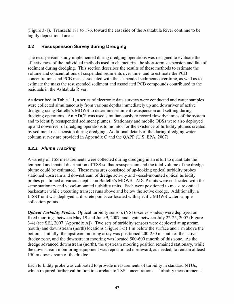
47

(Figure 3-1). Transects 181 to 176, toward the east side of the Ashtabula River continue to be highly depositional area. 3.2 Resuspension Survey during Dredging The resuspension study implemented during dredging operations was designed to evaluate the effectiveness of the individual methods used to characterize the short-term suspension and fate of sediment during dredging. This section describes the results of these methods to estimate the volume and concentrations of suspended sediments over time, and to estimate the PCB concentrations and PCB mass associated with the suspended sediments over time, as well as to estimate the mass the resuspended sediment and associated PCB compounds contributed to the residuals in the Ashtabula River. As described in Table 1.1, a series of electronic data surveys were conducted and water samples were collected simultaneously from various depths immediately up and downriver of active dredging using Battelle’s MDWS to determine sediment resuspension and settling during dredging operations. An ADCP was used simultaneously to record flow dynamics of the system and to identify resuspended sediment plumes. Stationary and mobile OBSs were also deployed up and downriver of dredging operations to monitor for the existence of turbidity plumes created by sediment resuspension during dredging. Additional details of the during-dredging water column survey are provided in Appendix C and the QAPP (U.S. EPA, 2007).

3.2.1 Plume Tracking

A variety of TSS measurements were collected during dredging in an effort to quantitate the temporal and spatial distribution of TSS so that resuspension and the total volume of the dredge plume could be estimated. These measures consisted of up-looking optical turbidity probes stationed upstream and downstream of dredge activity and vessel-mounted optical turbidity probes positioned at various depths on Battelle’s MDWS. ADCP units were co-located with the same stationary and vessel-mounted turbidity units. Each were positioned to measure optical backscatter while executing transect runs above and below the active dredge. Additionally, a LISST unit was deployed at discrete points co-located with specific MDWS water sample collection points. Optical Turbidity Probes. Optical turbidity sensors (YSI 6-series sondes) were deployed on fixed moorings between May 19 and June 9, 2007, and again between July 22-25, 2007 (Figure 3-4) (see SEI, 2007 [Appendix A]). Two sets of turbidity sensors were deployed at upstream (south) and downstream (north) locations (Figure 3-5) 1 m below the surface and 1 m above the bottom. Initially, the upstream mooring array was positioned 200-250 m south of the active dredge zone, and the downstream mooring was located 500-600 mnorth of this zone. As the dredge advanced downstream (north), the upstream mooring position remained stationary, while the downstream monitoring equipment was repositioned northward, as needed, to remain at least 150 m downstream of the dredge. Each turbidity probe was calibrated to provide measurements of turbidity in standard NTUs, which required further calibration to correlate to TSS concentrations. Turbidity measurements

48

were directly compared to TSS derived from water samples collected at the mooring locations at water depths consistent with optical turbidity probe mounting depths on May 19 and 31, June 4-5 and 7-10, and July 22-24, 2007.

Figure 3-4. Schematic Depicting the Stationary Turbidity Probe and ADCP Upstream and Downstream of Dredging Activities.

Concurrently collected NTU and TSS data were filtered for outliers by using 20-bin histograms to determine NTU and TSS frequency of occurrences (Figure 3-6) (Emery and Thomson, 1997). All negative values and values with a frequency of occurrence less than 5 were removed from the dataset. Least-square linear regression with forced zero intercept was then performed for NTU vs. TSS. The resulting best fit slope was 0.83. The correlation coefficient, r2, was 0.69 for data points within 1.25 standard deviations of the best fit line (Figure 3-6; in red) and r2 = 0.17 for all filtered data points (not shown). Time series of TSS were estimated from measured turbidity following:

TSSTURB.m = 0.83 * NTU (Equation 3-1) Common to long deployments of optical sensors in productive waters, the optical turbidity data suffered from biofouling. Hence, time series of turbidity-derived TSS were manually filtered to remove periods when data indicated that the optical sensor was obstructed. Data were also corrected for sensor calibration differences caused by different optical responses between the calibration standard and the in situ sediments by assuming minimum values of TSSTURB.m of 5 mg/L and 10 mg/L for near-surface data and near-bottom data, respectively. These values were based on near-bottom and near-surface TSS minimums determined by ADCP ABS.

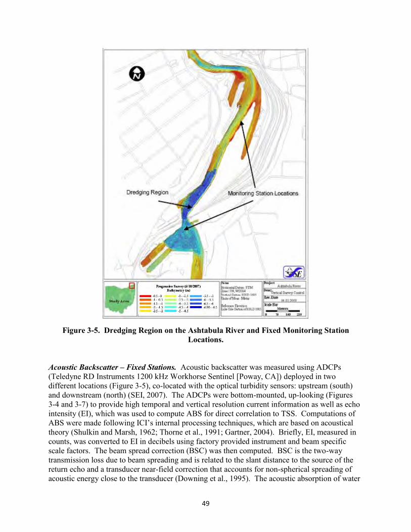
49

Figure 3-5. Dredging Region on the Ashtabula River and Fixed Monitoring Station Locations.

Acoustic Backscatter – Fixed Stations. Acoustic backscatter was measured using ADCPs (Teledyne RD Instruments 1200 kHz Workhorse Sentinel [Poway, CA]) deployed in two different locations (Figure 3-5), co-located with the optical turbidity sensors: upstream (south) and downstream (north) (SEI, 2007). The ADCPs were bottom-mounted, up-looking (Figures 3-4 and 3-7) to provide high temporal and vertical resolution current information as well as echo intensity (EI), which was used to compute ABS for direct correlation to TSS. Computations of ABS were made following ICI’s internal processing techniques, which are based on acoustical theory (Shulkin and Marsh, 1962; Thorne et al., 1991; Gartner, 2004). Briefly, EI, measured in counts, was converted to EI in decibels using factory provided instrument and beam specific scale factors. The beam spread correction (BSC) was then computed. BSC is the two-way transmission loss due to beam spreading and is related to the slant distance to the source of the return echo and a transducer near-field correction that accounts for non-spherical spreading of acoustic energy close to the transducer (Downing et al., 1995). The acoustic absorption of water

50

(WA) was calculated (Shulkin and Marsh, 1962) using ADCP measured temperature values and the freshwater assumption (salinity equal to zero). WA is related to the hydrographic properties of the water column and the slant distance to the source of the return echo. ABS was then computed following:

ABS = 10 log10(EI) + BS + WA (Equation 3-2)

Figure 3-6. Histograms to Determine Frequency of Occurrence for Turbidity (A), and TSS (B). (The outlier filtering criteria [values less than 0 or whose frequency of occurrence is less than 5] are indicated with red lines. Linear relationship between optical turbidity and TSS (C). The best

fit linear regression and 1.25 standard deviations of the best fit line are shown in blue.)

Resulting depth-resolved time series of ABS were correlated to TSS derived from water samples collected at the mooring sites on May 19 and 31, June 4-5 and 7-10, and July 22-24, 2007. A log-linear relationship was developed with co-located, concurrent ABS and TSS data (Figure 3-8). The least square log-linear regression fit was satisfactory with no data filtering performed. The resulting slope (m = 0.035) and intercept (b = -1.4) values are comparable to those obtained in other aquatic systems (riverine, estuarine, and coastal). The correlation coefficient, r2, for data within 1.25 standard deviations of the best fit line was 0.64; r2 = 0.31 for the full data set.

51

Figure 3-7. Up-looking Acoustic Doppler Current Profiler (ADCP) (Teledyne RD Instruments 1200 kHz Workhorse Sentinel ADCP [Poway, CA]) on Bottom-Mount Platform for Measuring

TSS.

Figure 3-8. Log-linear Relationship between ABS and TSS. (The best fit log-linear regression and 1.25 standard deviations of the best fit line are shown in red.)

Depth-resolved time series of TSS were derived from mooring derived ABS following:

TSSABS.m = 10(0.035 * ABS – 1.4) (Equation 3-3)

TSSABS.m as a function of depth as well as near-bottom TSSABS.m (bin 1) from the upstream (south) and downstream (north) mooring locations are shown in Figures 3-9 and 3-10. The general temporal variability of TSS derived from optical and acoustical methods is comparable (Figure 3-11).

52

Figure 3-9. A: Depth-Resolved Time Series of TSSABS.m Derived from ABS Computed from Echo Intensity Measured by the Upstream (South) Bottom-Mounted ADCP.

(The y-axis represents distance above transducer [meters]. B: TSSABS.m derived from ABS measured at bin 1, or nearest to the bottom [approximately 1 m above bottom]).

Acoustic Backscatter – Mobile Measurements. ABS was also computed from vessel-mounted ADCP transect data for comparison to TSS derived from optical turbidity sensors that were mounted on the Battelle MDWS. Vessel-mounted ADCP data were first gridded to a 3-m horizontal grid spacing and a 0.3-m vertical grid spacing to match the cell sizes of the TSS data derived from the optical turbidity sensors mounted on the MDWS (TSSTURB.MDWS). ABS data from the vessel-mounted ADCP were then computed from the gridded EI data, and TSS from the vessel-mounted ADCP (TSSABS.v) was estimated for each transect using the log-linear relationship obtained from moored ADCP data:

TSSABS.v = 10(0.035 * ABS – 1.4) (Equation 3-4)

The least square linear regression correlation coefficient between TSSABS.v and TSSTURB.MDWS was at times excellent (> 0.9) and at times poor (< 0.25). Poor relationships were generally found during periods of high frequency current direction shifts associated with Lake Erie seiche effects (SEI, 2007), which resulted in noisy ADCP EI signals (Figure 3-12; A and B). Excellent relationships were generally found during periods associated with constant flow direction (Figure 3-12; C and D). These results indicated that the use of boat-mounted ADCPs is suitable for aquatic systems with constant flow directions or lower frequency current direction shifts (e.g., river or tidal estuary) and is

53

an excellent method with which to obtain co-located TSS and current information with high temporal and spatial resolution.

Figure 3-10. A: Depth-Resolved Time Series of TSSABS.m Derived from ABS Computed from Echo Intensity Measured by the Downstream (North) Bottom-Mounted ADCP.

(The y-axis represents distance above the transducer. B: TSSABS.m derived from ABS measured at bin 1, or nearest to the bottom [approximately 1 m above bottom]).

Figure 3-11. Time Series of TSS Derived from Optical Turbidity (blue) and Acoustical Backscatter (ABS; red) for Data Collected at the Upstream (South) Site Comparing Methods

at about (A) 1 m below the Surface and (B) 1 m above the Bottom and for Data Collected at the Downstream (North) Site Comparing Methods at about (C) 1 m below the Surface and (D) 1 m

above the Bottom.

54

Figure 3-12. TSS as a Function of Cross-Channel Distance and Depth; Example Comparisons between TSS Derived from Optical Turbidity Measurements Collected on the MDWS (A and

C) and Acoustic Backscatter Measurements Collected from a Vessel-Mounted ADCP (B and D). ([A and B]) Illustrate a Poor Comparison Observed during Lake Erie Seiche Effects and [C and

D] Illustrate an Excellent Comparison Collected during Constant Flow.)

Laser In Situ Scattering and Transmissometry (LISST). A LISST instrument (Sequoia Scientific, Inc. 100X, type B ([Bellevue, WA)]) was deployed in the center of channel cross-sections for some of the transects measured with the ADCP and MDWS (SEI, 2007; Appendix A). The type B sensor measures the size distribution for particles between 1.4 and 231.0 µm in diameter using laser diffraction technology (Agrawal and Pottsmith, 1994).

LISST derived particle size distributions were converted to total volume concentration by summing the volume concentration (µL/L) of each particle size bin as derived by the instrument. The conversion of total volume concentration to TSS was then performed by comparing the LISST profile of total volume concentration (LISSTVC) to the TSS profile determined from optical turbidity sensors mounted on the MDWS (TSSTURB.MDWS) at the center point of the deepest part of the transect collected nearest in time to that of the LISST. Least square linear regression between total volume concentration and TSSTURB.MDWS (forced zero intercept) was used to determine the bulk particle density (p):

55

p (g/cm3) = m * LISSTVC + b (Equation 3-5) where m and b are the slope and intercept of the best-fit linear regression line between LISSTVC (µL/L) and TSSTURB.MDWS (mg/L). Although the correlation coefficients of the best fit between LISSTVC and TSSTURB.MDWS at times exceeded 0.9 (median r2 for all LISST profiles was 0.6; Figure 3-13), the LISST method to derive TSS was determined to be infeasible for this project. Resulting bulk particle density values (i.e., the slope of the best fit lines) ranged between 0.14 and 0.83 g/cm3, which were extremely low. The bulk density of inorganic particles is typically 2.65 g/cm3. The primary shortfall of using the LISST to derive TSS for this project was the assumption that all particles are in the size range as measured by the LISST, type B (between 1.4 and 231.0 µm) and that the bulk density of particles was constant with depth. Other limitations included:

Indeterminate sampling locations of the LISST profile relative to the TSS transect

Dissimilar sampling times of the LISST profile and MDWS transect.

Methods and Metrics for Identifying the Plume. The data used for the development of methods and metrics for identifying the dredge plume were TSS transects derived from optical turbidity data collected using the Battelle MDWS system (TSSTURB.MDWS) and depth-resolved time series of TSS estimated from the upstream (south) mooring ADCP data (TSSABS.m). Subsequent transects collected while progressing toward and away from the dredge operation area, hereafter referred to as progressive transects, were evaluated for plume signatures following the methods described below. The data ranged from sets of three to 10 transects collected from greater than 1000 m upstream to greater than 1000 m downstream of the dredge. Progressive transects were collected between May 31 and June 2 and between and June 4 and 10, 2007.

The first step necessary for identifying the dredge plume was to determine background TSS and subtract it from TSS collected during progressive transects, where:

TSSplume = TSSTURB.MDWS – TSSback. TSSback (Equation 3-6)

for each sampling day was assumed to be equal to the minimum values of TSSABS.m at each bin depth of the upstream (south) mooring ADCP recorded for each particular sampling day. In this manner, TSSback was allowed to vary with the environmental conditions of the Ashtabula River. The upstream (south) mooring was chosen because its water depth was greater than that at the downstream (north) mooring; therefore, it provided TSSback for a larger portion of the water column. The background TSS profile was interpolated to the MDWS measurement depths (between surface and 6 m with a grid spacing of 0.3 m) and subtracted from TSSTURB.MDWS at each vertical and horizontal grid cell. Negative values of TSSplume were not allowed, i.e., TSSback was set equal to TSSTURB.MDWS when TSSback was found to be greater than TSSTURB.MDWS. The major limitation in this method was that TSSback was assumed to be constant across-channel. Examples of TSSplume are shown in Figures 3-14 and 3-15 (more volumetric plots can be found in Appendix A).

56

Following plume identification, it was necessary to distinguish the dredge plume, TSSdredge, from elevated TSS levels from other sources, i.e., Lake Erie or Ashtabula River flow. TSSdredge was determined for each set of progressive transects by computing the along-shore gradient of TSSplume, where: TSSdredge = ∆TSSplume/∆x; ∆TSSplume is the change in TSSplume from one progressive transect to the next for each grid cell and ∆x is the along-channel distance from the center point of the dredge operating area to the location of the TSSTURB.MDWS transect. Transect distances upstream (south) of the dredge operating area were negative, and transect distances downstream (north) of the dredge operating area were positive (as shown in Figures 3-14 and 3-15); therefore, ∆x was always positive. A transect grid was created at the origin (i.e., the dredge site, where x = 0); TSSorigin was assumed to be equal to the maximum value of TSS collected over all TSSTURB.MDWS (≈140 mg/L).

Figure 3-13. LISST Measured Total Volume Concentration vs. TSS as Measured by the Optical Turbidity Sensors Mounted on the MDWS for LISST Profiles Corresponding to

MDWS Transects. (The best fit lines are shown for multiple measurements indicated by varied colors.)

A negative value of TSSdredge upstream of the dredge indicated that particular value of TSSplume originated from sources other than the dredge, i.e., Ashtabula River flow. Similarly, a positive value of TSSdredge downstream of the dredge area indicated elevated TSS originating from Lake Erie. In order to map only TSS originating from the dredge, TSS values associated with non-dredge related processes were set equal to zero.

Maps of Plume Extent during Identifiable Dredging Events. Dredge plume strength was computed from TSS values determined to originate from the dredge (non-zero values of TSSdredge). All positive values of TSSdredge upstream and the absolute value of all negative values

57

of TSSdredge downstream were normalized to the largest value of TSSdredge computed for all transects in a particular set of progressive transects:

NPS = |TSSdredge|/ |TSSdredge_max| (Equation 3-7) where NPS is “normalized plume strength”. An NPS value of 1.0 indicated strong dredge plume signature and an NPS of 0 indicated no dredge plume signature (Figures 3-16 through 3-19).

Figure 3-14. Three Dimensional Volumetric Plot of TSSplume Derived from TSSTURB.MDWS Progressive Transects Collected on June 2, 2007.

(The cross-shore distance was 60 m, and the along-shore distance covered by the transects was approximately 1200 m).

Figure 3-15. Three Dimensional Volumetric Plot of TSSplume Derived from TSSTURB.MDWS Progressive Transects Collected on June 5, 2007.

(The along-shore distance covered by the transects was approximately 2000 m.)

58

Figure 3-16. Normalized Plume Strength (NPS) as a Function of Cross-Channel Width and Water Depth Determined for Progressive Transects Collected on May 31, 2007.

The Dredge Region and Transect Locations by Number are Indicated on the Map. (The transect number and downstream distance from the dredge are indicated above each panel. Stronger dredge plume signatures are shown in red, and weaker signatures are shown

in blue; black indicates no dredge plume signature [NPS = 0]. Note the different NPS scales in each panel.)

59

Figure 3-17. 3-D Volumetric Plot of NPS for the Transects shown in Figure 3-16.

Estimates of the volume of water affected by dredge activity were calculated following the methods described here. Each transect in a set of progressive transects was evaluated for significant plume signature, which was defined as a grid cell exhibiting NPS greater than or equal to 0.1 or at least 10% of maximum TSSdredge. If no grid cells contained NPS values of at least 0.1 4F

3, the transect was not included in the calculations. Once all transects were evaluated, the cross-sectional area of each transect identified to contain significant plume signature(s) was computed. Cross-sectional areas were determined by: 1) calculating the width of each vertical bin through summation of the number of cross-channel grid cells containing data and multiplying by the horizontal grid cell spacing (3 m), 2) multiplying the width of each vertical bin by the vertical grid cell spacing (0.3 m), and 3) summing all areas (Figure 3-20A). Each transect’s cross-sectional area was then multiplied by the along-channel distance between it and the next transect identified to contain significant plume signature(s). The results were summed to estimate the total volume of water affected by the dredge (Figure 3-21A). This method assumes that the channel width remained constant between two subsequent progressive transects.

3 The value of 0.1 was chosen to represent error in TSS estimates. It is based on cumulative experience in estimating TSS from optical and acoustical backscatter. Note that this value of 0.1 is used as a minimum criterion to estimate the volume of water affected by dredge activity and the total volume of the dredge plume based on instantaneous transect data. It has no bearing on cumulative mass.

60

Figure 3-18. Normalized Plume Strength (NPS) as a Function of Cross-Channel Width and Water Depth Determined for Progressive Transects Collected on June 4, 2007.

The Dredge Region and Transect Locations by Number are Indicated on the Map. (The transect number and downstream distance from the dredge are indicated above each panel. Stronger dredge plume signatures are shown in red, and the weaker signatures are

shown in blue; black indicates no dredge plume signature [NPS = 0]. Note the different NPS scales in each panel.)

61

Figure 3-19. 3-D Volumetric Plot of NPS for the Transects shown in Figure 3-18.

Figure 3-20. Example Computations for the Cross-Sectional Area of A): A Transect Affected by the Dredge Plume; B): The Dredge Plume (cells containing significant plume

signature).

Similar computational procedures were followed in order to estimate the total volume of the dredge plume (Figure 3-21B). However, instead of calculating the width of each vertical bin through summation of the number of cross-channel grid cells containing data, the width of each vertical bin was determined by summing the number of grid cells containing NPS values greater than or equal to 0.1 (Figure 3-20B). Results indicate that the total volume of water affected by the dredge plume varied between approximately 30 m3 and 130 m3, and the total volume of the dredge plume varied between 20 m3 and 120 m3.

A B

62

Figure 3-21. Estimates of the A) Total Volume of Water Affected by the Dredge; B) Total Volume of the Dredge Plume.

(The upstream and downstream components of each volume estimate are also shown and labeled.)

3.2.2 Resuspended Sediment Mass

The rates generated for TSS by dredge activity and the estimates of mass transported away from the dredge operation were used to estimate resuspended mass at discrete time periods, as well as totaled over the entire dredging activity. Water Column Sediment Flux Calculations. Sediment fluxes were calculated using transect data collected repeatedly in the same location at a set distance from dredging activity over a sustained period of time, hereafter referred to as grouped transects. Ten sets of grouped transect data were collected between June 7 and 9, 2007. These data ranged from sets of three to 14 transects collected over periods of time between 20 minutes to greater than 2 hours. The locations of grouped transects were from more than 1000 m upstream to greater than 450 m downstream of the dredge. The current velocity from the vessel-mounted ADCP and TSS derived from optical turbidity sensors mounted on the MDWS were used to calculate water column sediment fluxes. Sediment flux was defined as follows:

F = Q * C, (Equation 3-8) where F is flux in units of mass per time, Q is flow rate in units of volume per time, and C is concentration in units of mass per volume. Therefore, it was necessary to compute Q using transect ADCP data and multiply derived Q with TSS to derive sediment flux. To avoid making assumptions about the direction of the boat traverse relative to the along-channel flow (i.e., eliminate the effects of boat crabbing) straight cross-channel transect lines normal to the river banks were used in the computations. These straight transect lines were determined by taking the average start and end points in each set of grouped transects and drawing a straight line

A B

63

between these two points. Unit vectors were calculated for the straight cross-channel line (representing the transect line) and the line normal to the cross-channel line (representing the flow line). This method assumed that on average, the boat’s start and end points were perpendicular to the channel. The flow rate of each measurement grid cell was then determined as follows:

dQ = U * dA, (Equation 3-9)

where U is the along-channel current velocity (see Equation 3-12) and dA is the area of the grid cell:

dA = dl * dz, (Equation 3-10)

where dl is the straight, cross-channel transect line and the vertical grid spacing is dz. The vertical grid spacing was always 0.3 m and:

dl = Sx * dlx + Sy * dly, (Equation 3-11)

where Sx and Sy were the east and north components of the transect line unit vector and dlx and dly were the east and north distances travelled by the boat as measured by the ADCP bottom track system. Similarly, the unit vector normal to the cross-channel transect line was used to compute the along-channel current velocity, U:

U = Nx * u + Ny * v, (Equation 3-12)

where Nx and Ny are east and north components of the flow line unit vector and u and v are the east and north components of current velocity as measured by the ADCP. Again, because unit vectors along and normal to a straight, cross-channel transect line were used, no assumptions were made about the direction travelled by the boat relative to the along-channel flow direction, and hence the effects of boat crabbing were eliminated.

The results for computations of dQ were validated by summing dQ over all grid cells to derive total flow rate for each measured transect. The sign of the flow rate was then compared to the velocity direction as measured by the North mooring ADCP. Positive flow rates represented downstream flow, and upstream flow was represented by negative Q (i.e., a right-hand coordinate system was used). With the exception of transects collected during or just after periods of high frequency directional shifts caused by the Lake Erie seiche effect, the flow rate directions were in agreement with current velocity directions recorded by the downstream (north) mooring ADCP.

Following validation of flow direction, total Q for each transect was computed by summing dQ of all cells along with the assumption that the values of dQ in cells affected by the near-surface ADCP blanking distance (1.02 m) were equal to the values of dQ in the uppermost measured bin. Sediment flux, F, was calculated by multiplying transect Q by the average value of TSSplume (TSSTURB.MDWS – TSSback) over all cells of each transect.

64

Estimates of TSS Generated by Dredge at Multiple Time Periods. The sediment fluxes determined for each transect in a group were integrated over the time period of grouped transect collection to derive Total Mass of Sediment (kg) per group (and per time period of grouped transect collection). This value was divided by the time passed during each particular grouped transect collection (in hours) to derive Total Mass of Sediment per hour. This was repeated for each of the 10 groups of transects.

In order to estimate the generation of TSS by the dredge, any values of Total Mass of Sediment that were determined to point toward the dredge, i.e. negative values downstream of the dredge and positive values upstream of the dredge, were assumed to be from factors other than dredging (e.g., natural Ashtabula River flow or Lake Erie seiche) and set equal to zero. All other values were determined to represent the total mass of dredge sediment per hour of dredging.

The absolute value of the total mass of dredge sediment per hour of dredge activity was plotted as a function of distance from dredge, and a power-law fit was applied to the trend (Figure 3-22). This enabled the prediction of sediment mass generated by the dredge as a function of distance from the dredge.

Figure 3-22. Absolute Value of the Total Mass of Dredge Sediment per Hour of Dredge Activity as a Function of Distance from the Dredge.

(The power-law fit to the data is shown and the equation is provided where X is distance from dredge.)

Estimates of Generation of TSS by Dredge as a Grand Total over the Entire Period of Dredging Activity. The estimated relationship between the total mass of dredge sediment per hour of dredge operation as a function of distance upstream and downstream from the dredge is

65

shown in Figure 3-22. This empirically-based function can be used to estimate the generation of TSS by the dredge. For example, at less than 25 m from the dredge, an average of 100 kg of sediment was measured during an hour of dredging time. This implies that during 8 hours of dredging, 800 kg of sediment were generated in the direct vicinity of the dredge operations. The grand total of TSS generation during the entire dredging activity can similarly be estimated for varying distances from the dredge. However, it should be noted that this does not necessarily reflect what mass has left the project area. For example, material that is resettled and subsequently dredged later is not quantified with the methodology outlined here.

Estimates of Generation of TSS by Dredge: Comparison with Analytic Methods. Predictions of the generation of solids mass by the dredge were accomplished by using the cutterhead dredge dimensional model presented by Hayes et al. (2000). The dimensional model was developed using stepwise regression analysis to determine empirical relationships between resuspended sediment data and cutterhead dredge operational and environmental variables. The following procedures were followed to predict the rate of sediment resuspended by the dredge, g (units of kg/hr):

The total surface area of the cutter, Ac, and the surface area of the cutter exposed during dredging, Ae, were computed.

Ac = (2 Lc dc) / 4 (Equation 3-13) Ae = Ac (Equation 3-14)

where Ac and Ae are in units of m2, Lc and dc are the length and diameter of the cutter (units of meters), respectively, for a 0.3 m cutterhead dredge, and is the proportion of the cutter that is exposed during dredging.

The rate of sediment resuspended by the dredge for port-to-starboard swings (gps; kg/hr) was calculated.

gps = 1.3147 | Vs – dc|1.864 [Ae / (dc Lc)]14.143 (Equation 3-15)

The rate of sediment resuspended by the dredge for starboard-to-port swings (gsp; kg/hr) was calculated.

gsp = 1.3147 | Vs + dc|1.864 [Ae / (dc Lc)]14.143 (Equation 3-16)

where Vs is the swing velocity at the tip of the cutter (m/s) and is the cutter rotation speed (rotations per second).

The rate of sediment resuspended by the dredge, g, was computed as the average of gps and gsp.

The operational and environmental variables used as input for the empirical model for a 12 in. cutterhead are presented in Table 3.2 (“Input”). Sensitivity analysis for the variables were investigated; upper and lower limits for the operational variables were determined following Hayes and Wu (2001) (Table 3.2; “Sensitivity Analysis”).

66

Table 3.2: Operational and Environmental Variables Used as Input for the Empirical Model to Determine the Rate of Sediment Resuspended by the Dredge.

Lc (m) dc (m) Vs (m/s) (rps) g (kg/hr)

Input 0.8 1.0 0.5 0.3 0.3 24.8

Sensitivity Analysis

0.8 1.0 0.35 – 0.65, every 0.02

0.05 – 0.65, every 0.05

0.1 – 0.5, every 0.033

0.16 (min) – 1015 (max)

The rate of sediment resuspended by the dredge determined by the empirical model of Hayes et al. (2000) was 24.8 kg/hr. This value is more than four times less than the dredge sediment resuspension rate determined from measurements (100 kg/hr at less than 25 m from the dredge). There are several potential sources of discrepancy, namely measurement bias and unknown operational variable information. Measurement bias could have been due to sediment that remained suspended in the water column that was advected upstream and downstream by the Lake Erie seiche effect. Thus, the sediment plume could have been evaluated repeatedly, resulting in a bias toward higher measured suspended sediment loads.

The operational and environmental variables used as input to the empirical model were estimated based on literature (Hayes et al., 2000; Hayes and Wu, 2001) and could have significant impact on predictions of the rate of sediment resuspended by the dredge. The effects of input variables were evaluated with sensitivity analysis (Figures 3-23 through 3-25). Results indicate that the proportion of cutter surface area exposed to dredging, , had the strongest effect on resuspension rate determinations. The rate of sediment resuspended by the dredge varied by nearly four orders of magnitude, from 0.16 kg/hr to greater than 1000 kg/hr for varying by only ±0.15 of 0.5 (Hayes et al., 2000 suggested = 0.5) and all other variables set equal to those presented in Table 3.2, “Input”. Cutter tip swing speed, VS, had the least effect on g; dredge resuspension rate varied between 23 kg/hr and 32 kg/hr for swing velocities between 0.05 m/s and 0.65 m/s. Dredge sediment resuspension rate was moderately affected by variations in cutter rotation speed, . Cutter rotation speed was varied between 6 rpm and 30 rpm (0.1 rps and 0.5 rps), resulting in resuspension rates between 5 kg/hr and 61 kg/hr.

Results from sensitivity analysis indicate that the measured rate of dredge resuspension within 25 m of the dredge of approximately 100 kg/hr was within values of resuspension rates determined by the empirical model presented by Hayes et al. (2000). It is important to note that measured rates of sediment resuspension are difficult to compare directly to estimates computed from analytical methods due to the lack of knowledge about the operational parameters as well as modifications to operational parameters over dredging time periods. It is certain that, for example, the proportion of cutter surface area exposed to dredging was not constant over the entire time period of dredging operations. As we would assume an even distribution of the solids over the area resuspension rates is observed.

67

Figure 3-23. Rate of Sediment Resuspended by the Dredge as a Function of the Proportion of Cutter Surface Area Exposed to Dredging, .

(All other operational variables used in the empirical model by Hayes et al. [2000] are indicated at the top of the plot.)

Figure 3-24. Rate of Sediment Resuspended by the Dredge as a Function of Cutter Tip Speed, Vs. (All other operational variables used in the empirical model by Hayes et al. [2000] are indicated

at the top of the plot.)

68

Figure 3-25. Rate of Sediment Resuspended by the Dredge as a Function of Cutter Rotation Speed, .

(All other operational variables used in the empirical model by Hayes et al. (2000) are indicated at the top of the plot.)

Estimates of Residual Solids Mass and Thickness Generated due to Resuspension. Residual solids mass generated by dredging activities can also be estimated from the empirical relationship shown in Figure 3-22. If we define that residual solids mass is dredge material in suspension at a distance of greater than 1000 m from dredge operations, then 1 hour of dredge operations resulted in less than 5 kg of residual solids mass.

In order to estimate the potential residual thickness generated by the dredge, the maximum generation rate of approximately 100 kg/hr from Figure 3-22 can be used to conduct an order of magnitude analysis. In this analysis, it is assumed that the 100 kg of sediment is evenly deposited along a small stretch of river with an area of 1,000 m2. Dividing the 100 kg of sediment generated each hour by a conservatively low dry surface sediment density typical of fine sediment (500 kg/m3) and by the area over which the sediment is deposited (10,000 m2), a deposition rate of 0.2 mm/yr is calculated. In a standard 8 to 10 hours/day of dredging, approximately 2 mm of residuals could be expected in a 10,000 m2 region of channel. It is important to note that the calculation represents the maximum solids generation measured and assumes that all the sediment deposits over a moderate area of the channel.

69

3.2.3 Link to Contaminant Distribution

Figures 3-26 and 3-27 show the tPCB(c) concentrations in water column samples that were collected at varying depths and distances from the dredge using the MDWS. These water sample data were collected over a period of 8 days in June and July 2007 at four different depths in the water column while dredging was occurring in the area. The water depths collected using the MDWS ranged from approximately 0.2 to 5.6 m. In the laboratory, water samples (approximately 2 L) were filtered through a glass fiber filter (pore size 1 μm) to create two fractions for analysis, a dissolved water sample that went through the filter and a particulate sample on the filter that was measured as a mass and then converted to a water volume based on the original water sample volume. The tPCB(c) concentrations in both the dissolved-phase (filtered) and particulate-phase (from the glass fiber filter) are shown for each station as a function of depth of the MDWS (upper surface, upper mid-water, lower mid-water, near bottom). In general, PCB concentrations increased with depth and decreased with increased distance from the dredge footprint. The tPCB(c) concentrations in the upper surface and upper mid-water samples are very similar and possibly represent general water column concentrations in this region not related to dredging activities. The near bottom and lower mid-water samples indicate that tPCB(c) concentrations increase with closer proximity to the dredge location. In general, the tPCB(c) concentrations in the dissolved fraction didn’t change throughout the four water column depths. The increased tPCB(c) concentrations observed in the particulate fraction was likely attributable to the increased TSS found nearer to the actual dredging activity. In addition, based on plume tracking studies discussed elsewhere in this report, TSS was found to be higher near the sediment surface, where hydraulic dredging was occurring, and decreased substantially near the surface. The fact that the dissolved concentrations did not appear to change with distance or depth is likely due to the fact that these particulates settled out relatively quickly after dredging activity stopped, therefore, not allowing the water column to equilibrate with the elevated particulate concentrations. This is evidenced by the observed data and represented by the power-law model shown in Figure 3-22. Further discussion regarding the relationship between TSS and particulates is presented below. Relationships between dissolved, particulate, and dissolved plus particulate PCB concentrations with TSS were determined for each of the four different sampling depths and for the total of all samples collected in the month of June; July data were excluded due to a lack of concurrent ADCP data. Least-squares linear regression analysis with a forced zero-intercept was used to quantify the correlations. The results of the linear correlations between PCB and TSS are shown in Figure 3-28.

Minimal depth-dependence was noted for the correlation between PCB and TSS. The strongest correlation was found for the dissolved plus particulate phase; the correlation coefficient was 0.7. Therefore, the resulting correlation determined for dissolved plus particulate PCB vs. TSS was used to estimate PCB mass in the water column for specific events and totaled during the entire dredging activity. Three-dimensional volumetric plume plots of estimated PCB concentrations can be found in Appendix A. The PCB dredge plume was determined using gradients of TSSplume, similar to methods described previously, and the relationship between dissolved plus particulate PCB and

70

TSS. Recall that the dredge plume, TSSdredge, was determined for each set of progressive transects by computing the along-shore gradient of TSSplume. A negative value of TSSdredge upstream of the dredge indicated that that particular value of TSSplume originated from sources other than the dredge, i.e. Ashtabula River flow. Similarly, a positive value of TSSdredge downstream of the dredge area indicated elevated TSS originating from Lake Erie. TSS values associated with non-dredge related processes were set equal to zero. The remaining values of TSSdredge were multiplied by the regression coefficient shown in Figure 3-28 (C) to derive PCBdredge (Figure 3-29).

Note: Stations are ordered from least to greatest distance from dredge (no distance data are available for Stations AR-116, AR-119, AR-121, AR-186, AR-209, AR-210, and AR-233).

Figure 3-26. tPCB(c) in MDWS Samples Collected “at Upper Surface” and “Upper Mid-Water” Water Depths from Each Station and Distance (meters) from Dredge from Selected

Stations. Note: If no symbol is shown next to a station, then that station was greater than 100 m from the

dredge.

71

Note: Stations are ordered from least to greatest distance from dredge (no distance data are available for Stations AR-116, AR-119, AR-121, AR-186, AR-209, AR-210, and AR-233).

Figure 3-27. tPCB(c) in MDWS Samples Collected at “Lower Mid-Water” and “Near Bottom” Water Depths from Each Station and Distance (m) from Dredge to Selected

Stations. Estimates of Generation of PCBs by Dredge at Multiple Time Periods. PCB fluxes were computed in a similar manner to sediment fluxes:

F = Q * CPCB (Equation 3-15)

where F is flux in units of mass per time, Q is flow rate in units of volume per time, and CPCB is PCB concentration in units of mass per volume. CPCB was estimated based on the linear regression between TSS and dissolved plus particulate PCB concentration:

PCB (ng/L) = 12.6 * TSSplume (mg/L) (Equation 3-16)

72

where TSSplume is TSSback subtracted from measured TSSTURB.MDWS for each transect. PCB values derived from TSS were converted from units of ng/L to mg/L, averaged over each transect, then multiplied by Q. PCB fluxes calculated for each transect in a group were integrated over the time period of grouped transect collection to derive total mass of PCBs (g) per group (and per time period of grouped transect collection). This value was divided by the time passed during each particular grouped transect collection (in hours) to derive total mass of PCBs per hour. This was repeated for each of the 10 groups of transects.

Figure 3-28. Linear Relationships between PCB Concentration and TSS for the (A) Dissolved, (B) Particulate, and (C) Dissolved Plus Particulate Phases of PCB.

(The four sample collection depths are denoted by different colored symbols: near-bottom = blue, lower mid-water = green, upper mid-water = yellow, and near-surface = red. Least-squares

linear regressions for all depths are shown in black with 95% confidence limits in gray. Regression and correlation coefficients are indicated.)

A B

C

73

Figure 3-29. Volumetric Plot of the PCB Plume, Estimated from the Linear Relationship between Dissolved Plus Particulate PCB Concentration and TSS and MDWS and ADCP

Transect Data Collected on June 4, 2007. (The cross-shore distance was 60 m, and the along-shore distance covered by the transects was

approximately 1000 m [negative distances are upstream of the dredge and vice versa].)

In order to estimate the generation of PCBs by the dredge, any values of Total Mass of PCBs that were determined to point toward the dredge, i.e., negative values downstream of the dredge and positive values upstream of the dredge, were assumed to be from factors other than dredging (e.g., natural Ashtabula River flow) and set equal to zero. All other values were determined to represent the total mass of dredge PCB per hour of dredging.

The absolute value of the total mass of dredge PCBs per hour of dredge activity was plotted as a function of distance from dredge, and a power-law fit was applied to the trend (Figure 3-30). This enabled the prediction of PCB mass generated by the dredge as a function of distance from the dredge.

Estimates of Residual PCB Mass Generated Due to Resuspension. PCB residual solids mass generated by dredging activities can also be estimated from the empirical relationship shown in Figure 3-30. Assuming that residual solids mass is defined as dredge material in suspension at a distance of greater than 1000 m from dredge operations, then 1 hour of dredge operations resulted in less than 0.06 g of PCB residual solids mass. Two hours of dredge activities thus generated less than 0.12 g of PCB residual solids mass.

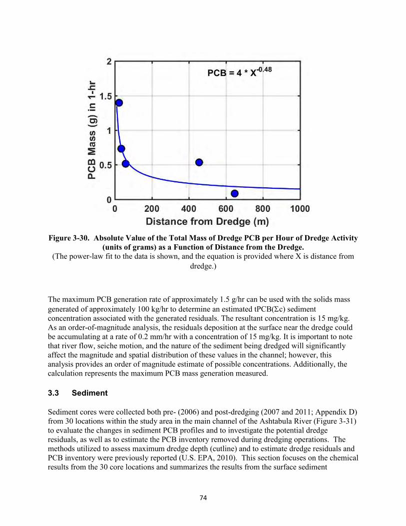
74

Figure 3-30. Absolute Value of the Total Mass of Dredge PCB per Hour of Dredge Activity (units of grams) as a Function of Distance from the Dredge.

(The power-law fit to the data is shown, and the equation is provided where X is distance from dredge.)

The maximum PCB generation rate of approximately 1.5 g/hr can be used with the solids mass generated of approximately 100 kg/hr to determine an estimated tPCB(c) sediment concentration associated with the generated residuals. The resultant concentration is 15 mg/kg. As an order-of-magnitude analysis, the residuals deposition at the surface near the dredge could be accumulating at a rate of 0.2 mm/hr with a concentration of 15 mg/kg. It is important to note that river flow, seiche motion, and the nature of the sediment being dredged will significantly affect the magnitude and spatial distribution of these values in the channel; however, this analysis provides an order of magnitude estimate of possible concentrations. Additionally, the calculation represents the maximum PCB mass generation measured. 3.3 Sediment Sediment cores were collected both pre- (2006) and post-dredging (2007 and 2011; Appendix D) from 30 locations within the study area in the main channel of the Ashtabula River (Figure 3-31) to evaluate the changes in sediment PCB profiles and to investigate the potential dredge residuals, as well as to estimate the PCB inventory removed during dredging operations. The methods utilized to assess maximum dredge depth (cutline) and to estimate dredge residuals and PCB inventory were previously reported (U.S. EPA, 2010). This section focuses on the chemical results from the 30 core locations and summarizes the results from the surface sediment

75

characterization efforts: 1) conducted herein, and 2) in conjunction with other discrete investigations concerning potential ongoing sources and post-dredging surface surveys as further outlined in Table 3.3. Surface sediments (generally 10 to 15 cm in depth) that were collected from other locations throughout the river in conjunction with ecosystem-related measurements (biological and passive samplers) are presented in Sections 3.4 and 3.5, respectively, along with the results from the co-located measurements.

Figure 3-31. Sediment Core Sample Locations in the Ashtabula River Study Area (Pre- and Post-Dredging).

Red line indicates the boundary of the GLLA project area.

3.3.1 Comparison of tPCB(c) Concentrations in Pre- and Post-Dredge Cores

Figures 3-32 through 3-39 compare tPCB(c) concentration profiles in cores collected pre-dredge (2006) and post-dredge (2007 and 2011). The color-coded dashed lines across each figure represent the sediment surface elevations at the time the cores were collected. Pre-dredge surface sediment elevations occur (in most cases) 0.15 m above the highest elevation identified in each figure, as each point represented on a figure is the midpoint of the core segment that was analyzed (i.e., the top core interval analyzed in the 2006 pre-dredge cores was 0.3 m). The tPCB(c) concentrations are based on the sum of 117 PCB congeners; congeners that comprise more than 98% of the total PCBs in all Aroclors and most environmental PCB contamination. The set of 117 PCB congeners (including co-reported co-eluting congeners) that were common

76

to all four sampling events were used to produce the tPCB(c) to be able to compare results. The method detection limit is included in the summation for congeners that were not detected. In general, the pre-dredge cores (shown in red; 2006) were collected at an elevation of 163 to 173 IGLD85 m and to a depth of approximately 5.5 to 7 m. Complications from year-to-year from leaf mats, debris, etc. caused deviations from the goal of year-to-year comparisons in some cases. Subsequent core collections targeted elevations below the project cut line to permit for year-to-year comparisons. Nonetheless, the 2007 post-dredge cores (shown in blue) were collected at an elevation of 166 to 170 IGLD85 m and to a depth of approximately 0.8 to 0.9 m. These 2007 cores revealed significant increases in PCB concentration, which is consistent with other observations here and as expected given the dredged residuals profile reported in U.S. EPA (2010). Note that in some cases, the 2007 sediment surface elevation increased as much as 0.6 m in sampling locations and as much as 3 m at T181D due to high sedimentation rates in that portion of the river as noted in Section 3.1. Leaf litter and other detritus made it difficult to obtain a deeper 2007 core sample at T181D. Increased PCB concentrations at approximately mid-depth at all transect locations and negligible or low PCB concentrations at maximum depth were observed.

In 2011, cores were collected at an elevation of 166.5 to 170 IGLD85 m. Surface sediment PCB concentrations had returned to pre-dredge levels or lower due to significant sedimentation of cleaner sediments from 2007 to 2011. The exception was at T178B where far less sedimentation was observed relative to all other sample locations.

77

Elevation = IGLD85 meters

Figure 3-32. tPCB(c) Concentrations (mg/kg) in Pre- (2006) and Post-Dredge (2007 and 2011) Cores at Transects 170 and 171 (A = West Side of River, B = East Side of River).

10-2

10-1

100

101

102

165

166

167

168

169

170

171

172

173

174

Ele

va

tio

n(m

)Station

T170A

2006 2007 2011

10-2

10-1

100

101

102

164

165

166

167

168

169

170

171

172

173

174

Ele

va

tio

n(m

)

Station

T170B

2006 2007 2011

10-2

10-1

100

101

102

165

166

167

168

169

170

171

172

173

174

Ele

va

tio

n(m

)

Station

T171A

2006 2007 2011

10-2

10-1

100

101

102

164

165

166

167

168

169

170

171

172

173

174

Ele

va

tio

n(m

)

Station

T171B

2006 2007 2011

78



10-2

10-1

100

101

102

165

166

167

168

169

170

171

172

173

174

Ele

va

tio

n(m

)Station

T172A

2006 2007 2011

10-2

10-1

100

101

102

164

165

166

167

168

169

170

171

172

173

Ele

va

tio

n(m

)

Station

T172B

2006 2007 2011

10-2

10-1

100

101

102

164

165

166

167

168

169

170

171

172

173

174

Ele

va

tio

n(m

)

Station

T173A

2006 2007 2011

10-2

10-1

100

101

102

164

165

166

167

168

169

170

171

172

173

Ele

va

tio

n(m

)

Station

T173B

2006 2007 2011

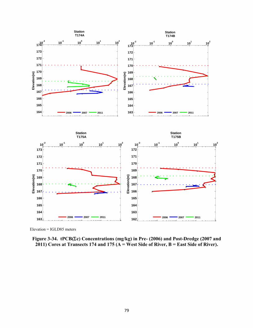
79



10-2

10-1

100

101

102

164

165

166

167

168

169

170

171

172

173

174

Ele

va

tio

n(m

)Station

T174A

2006 2007 2011

10-2

10-1

100

101

102

163

164

165

166

167

168

169

170

171

172

173

Ele

va

tio

n(m

)

Station

T174B

2006 2007 2011

10-2

10-1

100

101

102

163

164

165

166

167

168

169

170

171

172

173

Ele

va

tio

n(m

)

Station

T175A

2006 2007 2011

10-2

10-1

100

101

102

162

163

164

165

166

167

168

169

170

171

172

Ele

va

tio

n(m

)

Station

T175B

2006 2007 2011

80



10-2

10-1

100

101

102

162

163

164

165

166

167

168

169

170

171

172

Ele

va

tio

n(m

)Station

T176A

2006 2007 2011

10-2

10-1

100

101

102

164

165

166

167

168

169

170

171

172

173

Ele

va

tio

n(m

)

Station

T176B

2006 2007 2011

10-2

10-1

100

101

102

162

163

164

165

166

167

168

169

170

171

172

Ele

va

tio

n(m

)

Station

T177A

2006 2007

10-2

10-1

100

101

102

166

167

168

169

170

171

172

173

174

175

176

Ele

va

tio

n(m

)

Station

T177B

2006 2007 2011

81


Figure 3-36. tPCB(c) Concentrations (mg/kg) in Pre- (2006) and Post-Dredge (2007 and 2011) Cores at Transect 178 (A = West Side of River, B = Middle of River, C = East Side of

River).

10-2

10-1

100

101

102

162

163

164

165

166

167

168

169

170

171

172

Ele

va

tio

n(m

)Station

T178A

2006 2007 2011

10-2

10-1

100

101

102

163

164

165

166

167

168

169

170

171

172

173

Ele

va

tio

n(m

)

Station

T178B

2006 2007 2011

10-2

10-1

100

101

102

166

167

168

169

170

171

172

173

174

175

176

Ele

va

tio

n(m

)

Station

T178C

2006 2007 2011

82


Figure 3-37. tPCB(c) Concentrations (mg/kg) in Pre- (2006) and Post-Dredge (2007 and 2011) Cores at Transect 179 (A = West Side of River, B = Middle of River, C = East Side of

River).

10-2

10-1

100

101

102

162

163

164

165

166

167

168

169

170

171

172

Ele

va

tio

n(m

)Station

T179A

2006 2007

10-2

10-1

100

101

102

165

166

167

168

169

170

171

172

173

174

175

Ele

va

tio

n(m

)

Station

T179B

2006 2007 2011

10-2

10-1

100

101

102

166

167

168

169

170

171

172

173

174

175

176

Ele

va

tio

n(m

)

Station

T179C

2006 2007 2011

83


Figure 3-38. tPCB(c) Concentrations (mg/kg) in Pre- (2006) and Post-Dredge (2007 and 2011) Cores at Transect 180 (A = West Side of River, B = West Middle of River, C = East

Middle Side of River, D = East Side of River).

10-2

10-1

100

101

102

163

164

165

166

167

168

169

170

171

172

173

Ele

va

tio

n(m

)Station

T180A

2006 2007 2011

10-2

10-1

100

101

102

164

165

166

167

168

169

170

171

172

173

Ele

va

tio

n(m

)

Station

T180B

2006 2007 2011

10-2

10-1

100

101

102

166

167

168

169

170

171

172

173

174

175

176

Ele

va

tio

n(m

)

Station

T180C

2006 2007 2011

10-2

10-1

100

101

102

166

167

168

169

170

171

172

173

174

175

176

Ele

va

tio

n(m

)

Station

T180D

2006 2007 2011

84


Figure 3-39. tPCB(c) Concentrations (mg/kg) in Pre- (2006) and Post-Dredge (2007 and 2011) Cores at Transect 180 (A = West Side of River, B = West Middle of River, C = East

Middle Side of River, D = East Side of River). 3.3.2 Surface Sediment PCBs Trends

Shown in Table 3.3 are surface sediment tPCB(c) concentration data for 2006, 2007, and 2011 and the surface sediment segment interval that was analyzed based on visual observations of the cores and distinct horizons to be analyzed to target residuals in 2007 and recently deposited

10-2

10-1

100

101

102

164

165

166

167

168

169

170

171

172

173

174

Ele

va

tio

n(m

)Station

T181A

2006 2007 2011

10-2

10-1

100

101

102

163

164

165

166

167

168

169

170

171

172

173

Ele

va

tio

n(m

)

Station

T181B

2006 2007 2011

10-2

10-1

100

101

102

162

163

164

165

166

167

168

169

170

171

Ele

va

tio

n(m

)

Station

T181C

2006 2007 2011

10-2

10-1

100

101

102

161

162

163

164

165

166

167

168

169

170

171

Ele

va

tio

n(m

)

Station

T181D

2006 2007 2011

85

sediment in 2011. tPCB(c) concentrations are plotted in Figure 3-40, and surface contours of the pre- and post-dredge events are shown Figures 3-41 through 3-43, respectively. All surface contouring was conducted using a grid method/program, the EarthVision 2D Minimum Tension gridding algorithm, and a 20 ft by 20 ft grid spacing. The 2006 tPCB(c) surface sediment concentrations were variable across all sample locations and averaged 1.12 mg/kg. Seven stations (T174A, T176B, T178A, T179B, T179C, T180D, and T181B) had tPCB(c) surface concentrations greater than 1.00 mg/kg, including T176B with the highest concentration of 8.61 mg/kg. These sampling locations were in moderate to high depositional zones within the study area (U.S. EPA, 2010).

Table 3.3: tPCB(c) Concentrations (mg/kg) of Surface Sediment from Pre-Dredge (2006), Post-Dredge (2007), and Post-Dredge (2011).

Sediment Core ID

Pre-Dredge 2006 Post-Dredge 2007 Post-Dredge 2011 Segment Length

(m)

tPCB(c) (mg/kg

dry)

Segment Length

(m)

tPCB(c) (mg/kg

dry)

Segment Length

(m)

tPCB(c) (mg/kg

dry) T170A 0.3 0.581 0.06 4.29 0.2 0.188 T170B 0.3 0.734 0.09 5.71 0.09 0.211 T171A 0.3 0.641 0.03 18.9 0.2 0.190 T171B 0.18 0.224 0.06 37.7 0.2 0.275 T172A 0.3 0.652 0.09 20 0.2 0.210 T172B 0.3 0.209 0.05 4.57 0.2 0.526 T173A 0.3 0.849 0.03 4.09 0.2 0.276 T173B 0.3 0.369 0.06 4.65 0.2 0.454 T174A 0.3 1.14 0.06 3.35 0.2 0.258 T174B 0.3 0.235 0.01 8.34 0.2 0.125 T175A 0.2 0.175 0.05 12.0 0.2 0.267 T175B 0.1 0.152 0.03 7.01 0.2 0.121 T176A 0.2 0.495 0.1 3.21 0.2 0.340 T176B 0.3 8.61 0.02 6.51 0.2 0.0762 T177A 0.2 0.430 0.2 7.06 NA NA T177B 0.3 0.740 0.03 10.2 0.2 0.479 T178A 0.3 3.32 0.05 4.44 0.2 1.42 T178B 0.2 0.427 0.2 8.89 0.2 1.02 T178C 0.3 0.890 0.09 14.1 0.2 0.228 T179A 0.3 0.203 0.1 1.48 NA NA T179B 0.3 1.82 0.06 9.16 0.2 0.143 T179C 0.3 1.25 0.02 7.04 0.2 0.312 T180A 0.3 0.162 0.2 0.651 0.1 0.207 T180B 0.3 0.284 0.09 11.1 0.2 0.186 T180C 0.3 0.540 0.03 12.9 0.2 0.658

Table 3.3 (continued): tPCB(c) Concentrations (mg/kg) of Surface Sediment from Pre-Dredge (2006), Post-Dredge (2007), and Post-Dredge (2011).

86

Sediment Core ID

Pre-Dredge 2006 Post-Dredge 2007 Post-Dredge 2011 Segment Length

(m)

tPCB(c) (mg/kg

dry)

Segment Length

(m)

tPCB(c) (mg/kg

dry)

Segment Length

(m)

tPCB(c) (mg/kg

dry) T180D 0.3 3.12 0.03 7.35 0.2 0.575 T181A 0.3 0.587 0.1 1.18 0.2 0.0371 T181B 0.3 3.13 0.09 2.62 0.2 0.0859 T181C 0.3 0.821 0.05 4.93 0.2 1.17 T181D 0.3 0.744 0.09 11.2 0.2 0.561 Minimum -- 0.152 -- 0.651 -- 0.0371 Maximum -- 8.61 -- 37.7 -- 1.42 Average -- 1.12 -- 8.48 -- 0.379

NA = No data available. No sediment core collected.

Figure 3-40. Surface Sediment tPCB(c) Concentration (mg/kg dry) from Pre-Dredge (2006) and Post-Dredge (2007 and 2011).

The 2011 surface concentrations (average tPCB(c) was 0.379mg/kg) were almost three times (2.95) lower than the 2006 surface concentrations (1.12 mg/kg). The areas with the highest concentration of PCBs in 2006 (concentrations greater than 1.0 mg/kg) were less than 0.20 mg/kg in 2011.

0

2

4

6

8

10

12

14

16

18

20

22

T17

0A

T17

0B

T17

1A

T17

1B

T17

2A

T17

2B

T17

3A

T17

3B

T17

4A

T17

4B

T17

5A

T17

5B

T17

6A

T17

6B

T17

7A

T17

7B

T17

8A

T17

8B

T17

8C

T17

9A

T17

9B

T17

9C

T18

0A

T18

0B

T18

0C

T18

0D

T18

1A

T18

1B

T18

1C

T18

1D

tPC

B(

c) (

mg/

kg d

ry)

Station ID

2006 2007 2011

*T171B 2007 = 38 mg/kg dry

*

87

The percent fines in the surface sediment samples was variable across the 30 sediment cores. For example, the percent fines ranged from 14.3% to 99.8% across all locations and years (2006, 2007, and 2011), with an average of 73.1%. Examination of the cores from 2006 indicate that pre-dredge surface sediments consisted generally of stratified sand and clay, with the deeper intervals comprised mainly of clay silt and then clay before reaching the bedrock layer (Appendix D). In 2007, the sediment cores were characterized as being mainly clay mixed with silt or fine sandy clay. Although not analyzed for tPCB(C), 2009 sediment cores were comprised of mostly clay silt with traces of fine sand and organic matter (i.e., leaf matter). In 2011, fine sandy clayey silt with surface organic matter dominated the sediment type in the cores collected. Therefore, over time, there appeared to be a slight fining in surface sediments from pre-dredge (2006) to post-dredge (2007, 2009, and 2011) collections. This change in sediment characteristics would be expected as a result of the changes in the velocity profiles across the channel after dredging.

The TOC concentrations in the surface sediments were also variable ranging from 0.39% to 6.48%, with an average of 2.57%. A common means of assessing these bulk sediment properties is to represent the sediment grain size (as percent fines) vs. TOC under the premise that grain size relates to TOC. The Ashtabula River bulk sediment properties showed the expected positive slope, but the correlation was not a strong one (R2 = 0.127). The correlation between PCB concentrations and percent fines in the sediment samples was even weaker (R2 = 0.0844). Note that in all cases the data were highly variable, hence the confidence in the suggested correlations is low. No relationship was observed, and these data are presented in Appendix F.

Table 3.4 shows the average tPCB(c) concentrations in the surface segment from sediment cores collected in 2006, pre-dredging in 2007, post-dredging in 2007, and in 2011 (4 years post-dredging). Because the focus of the sediment collections was to target residuals in 2007 and recently deposited sediment in 2011, the sediment depth that the surface segment represented varied, making it challenging to interpret both the PCB concentration and PCB composition data.

The surface sediment samples collected before dredging had comparable average PCB concentrations in 2006 and 2007 (1.12 and 1.41 mg/kg, respectively). The surface sediment PCB concentrations were much higher shortly after dredging (averaged 8.37 mg/kg) compared to before dredging, which can most likely be attributed to dredged residuals with significant contributions from the highly contaminated sediments dredged from depth (generally 2-3 m) in 2007; the sediments from all depths that were dredged were mixed during the dredging operations, and some were re-deposited as surface sediment. These results and this phenomenon were previously discussed in the U.S. EPA 2010 report. The average surface sediment tPCB(c) concentrations were significantly lower in 2011 (averaged 0.358 mg/kg), indicating that sediments with lower PCB concentrations have been deposited in the study area after dredging. This sediment deposition was supported by a bathymetric survey conducted over the project area (Section 3.1), which measured an average of 0.16 m of deposition since 2007 (Table 3.1).

88

Figure 3-41. Surface Sediment tPCB(c) Concentrations from 2006 (Pre-Dredge); Created by EarthVision 2D Minimum Tension Gridding Algorithm using a 6.1-m x 6.1-m (20-ft x

20-ft) Grid Spacing.

MAX = 8.61 mg/kg

tPCB(c)

0.0

89

Figure 3-42. Surface Sediment tPCB(c) Concentrations from Cores Collected in 2007 (1 Year Post-Dredge); Created by EarthVision 2D Minimum Tension Gridding Algorithm

using a 6.1-m x 6.1-m (20-ft x 20-ft) Grid Spacing.

tPCB(c)

0.0

MAX = 37.7 mg/kg

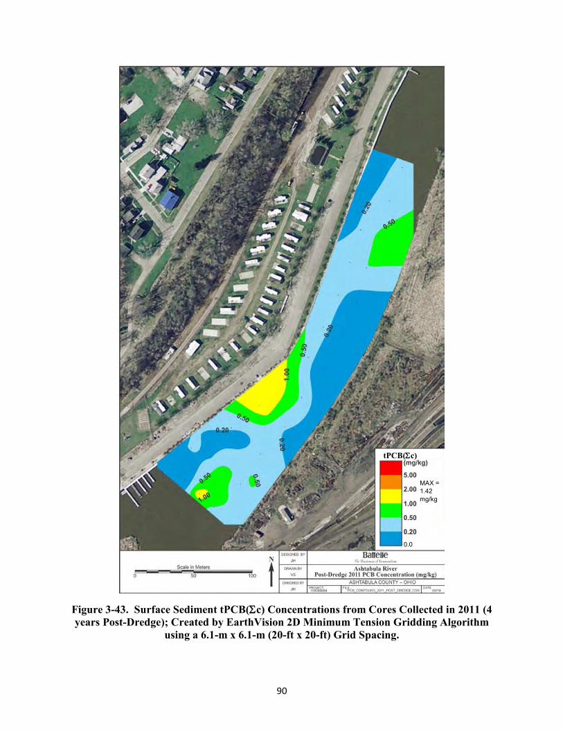
90

Figure 3-43. Surface Sediment tPCB(c) Concentrations from Cores Collected in 2011 (4 years Post-Dredge); Created by EarthVision 2D Minimum Tension Gridding Algorithm

using a 6.1-m x 6.1-m (20-ft x 20-ft) Grid Spacing.

tPCB(c)

0.0

MAX = 1.42 mg/kg

91

Table 3.4: Average tPCB(c) Concentrations (mg/kg) for 30 Surface Sediment Samples Collected in the Ashtabula River Study Area during Four Study Phases (two before

dredging and two after dredging).

Sampling Year/Event

tPCB(c) Concentration

(mg/kg, dry weight) Average Depth of

Samples (m)

No. of Samples (coring

locations) 2006 1.12 0.3 30 2007 Pre-Dredging (surface grabs) 1.41

0.1 20

2007 Post-Dredging 8.37 0.1 30 2011 0.358 0.2 33(a) (a) Includes five duplicates; the samples were from 28 locations.

The PCB composition, which was similar for the four different surface sediment sample sets, was consistently dominated by the historic Aroclor 1248 PCB source. This was the case with the 2006 samples and the 2007 samples collected both before and after dredging as described earlier (U.S. EPA, 2010). This was also the case for the samples collected in 2011 that are included with the 2006 and 2007 samples in the principal component analysis (PCA) shown in Figure 3-44. The PCA in Figure 3-44 was computed using PCB congener data; similar results were obtained using PCB homolog data. The PCA does not show any clear separation of samples by sampling event, indicating that the Aroclor 1248 source is the primary contributor to the PCB in all of these samples including the less contaminated sediments deposited in recent years. The few samples shown in Figure 3-44 that are separated from the main sample cluster in the PCA are samples with low PCB concentrations that include an unusually high relative contribution from PCB209; they also represent samples from various sampling events.

Other sampling and data analysis also indicated a contribution of Aroclor 1260 to the surface sediments in the main stem of the river before dredging. That contribution of Aroclor 1260 now has been shown to be detectable only in the confluence of Strong Brook and the Upper Turning Basin area; it no longer appears to be detectable in the sediments farther downstream (U.S. EPA, 2012). The ability to detect recent contributions from a second source was only possible using data for shallow surface sediment samples from the top few centimeters of sediment. The “surface sediment” data from the sediment cores illustrated in Table 3-5 and Figure 3-44 were collected to a depth from 0.1 to 0.3 m, on average, for the four sampling events and represent longer and differing time periods. This greater sampling depth makes it difficult to compare the data from the different sampling events to each other, and it also presents problems in distinguishing between current and recent contamination. It is therefore recommended the top 0.03 m consistently be isolated for analysis in future studies that include coring in different years, and that other core segmenting strategies (e.g., based on observations) be applied to the remaining sediment below 0.03 m depth.

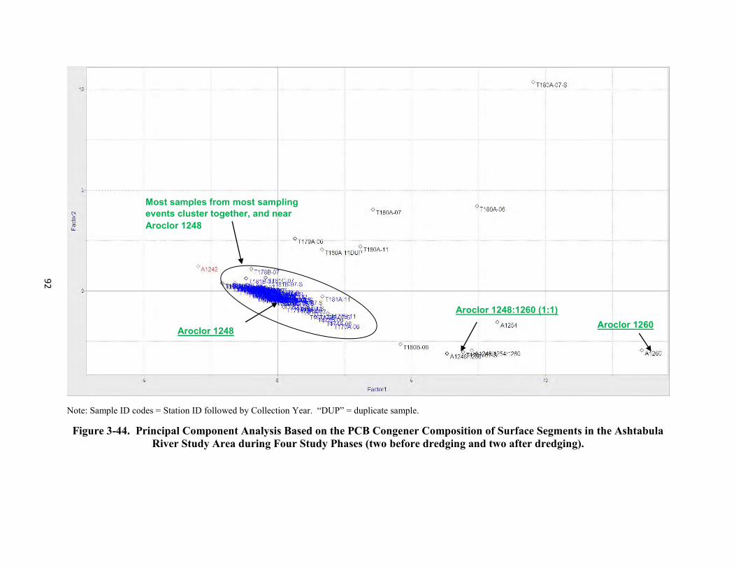
92

Note: Sample ID codes = Station ID followed by Collection Year. “DUP” = duplicate sample.

Figure 3-44. Principal Component Analysis Based on the PCB Congener Composition of Surface Segments in the Ashtabula River Study Area during Four Study Phases (two before dredging and two after dredging).

Aroclor 1248

Most samples from most sampling events cluster together, and near Aroclor 1248

Aroclor 1260 Aroclor 1248:1260 (1:1)

93

3.3.3 General Surface Sediment PCB Trends

In addition to the primary data sets collected to accomplish specific objectives specified in Section 2, further efforts were pursued throughout the project time span of this ORD study that were jointly executed by U.S. EPA ORD and U.S. EPA GLNPO. The data accumulated from four of these efforts are related and relevant to the understanding of the surface sediment conditions (as of 2011) beyond the ORD Study Area boundaries and encompass a surface sediment interpretation of the entire GLLA dredge footprint. Table 3.5 outlines the four primary investigations that were used to make the interpretations discussed in this section. The tPCB(c) concentrations in the 79 surface sediment samples from Studies 1 through 4 are presented in Table 3.6, along with TOC concentrations and the TOC-normalized tPCB(c) concentrations; this includes the samples representing the upper segment of the eight cores collected in Study 3. The tPCB(c) (and TOC and TOC-normalized tPCB(c)) concentrations of all 37 samples from the eight Study 3 sediment cores are presented in Appendix C. The tPCB(c) and TOC concentrations are presented geographically in Figures 3-45 and 3-46, respectively. Figures 3-47 and 3-48 show the concentration-extrapolated estimated tPCB(c) and TOC-normalized tPCB(c) concentrations, respectively. The tPCB(c) data for the Studies 1-3 samples are based on Aroclors, and the Study 4 data are based on PCB congeners. It should be noted that the two-dimensional concentration contours in Figures 3-47 and 3-48 are modeled concentrations. The contouring is highly dependent on the data extrapolation algorithms, the physical shape of the area being contoured, and the concentration distribution. These contoured representations should only be used to obtain an estimate of the concentrations and may not accurately represent the concentrations across the full area being depicted. The PCB and TOC concentrations at the specific station locations are the only concentrations that are known, and those are presented in Table 3.7.

94

Figure 3-45. Surface Sediment (top 0.15 m) tPCB(c) Concentrations (mg/kg, dry wt).

tPCB(c) (mg/kg)

95

Figure 3-46. Surface Sediment (top 0.15 m TOC (%) Concentrations.

96

Figure 3-47. Surface Sediment (top 0.15 m) tPCB(c) Concentration Approximation Contours (mg/kg, dry wt) Data.

tPCB(c) (mg/kg)

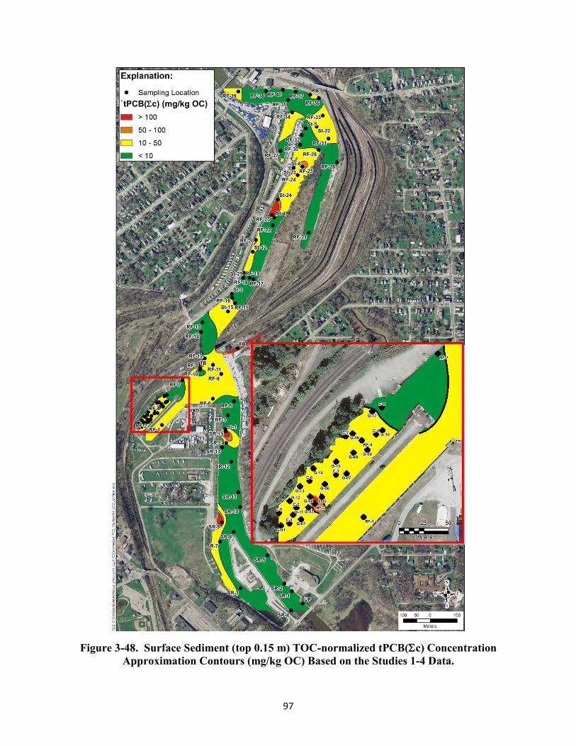
97

Figure 3-48. Surface Sediment (top 0.15 m) TOC-normalized tPCB(c) Concentration Approximation Contours (mg/kg OC) Based on the Studies 1-4 Data.

tPCB(c) (mg/kg OC)

98

Table 3.5: Sample Data used to Characterize General River Surface Sediment Trends.

Study Number and Data Sources # Sites/ Samples

PCB Aroclor

PCB Congeners

Surface sediment (top 0.15 m) samples collected in 2011 to calculate surface weighted average concentration at 54 locations throughout Ashtabula River and analyzed for PCB Aroclors, including from the area at the confluence of Strong Brook and the Ashtabula River, the Turning Basin, the mouth of Fields Brook, and upstream and downstream. These are Stations 40 RF (RF-1 through RF-40) and 14 SR (SR-1 through SR-15; no SR-6) stations, and samples with ER sample IDs. GLNPO Data. (see Appendix C of this report)

54 X

Surface sediment samples (top 0.15 m) collected in 2011 at 17 locations in the area at the confluence of Strong Brook and the Ashtabula River and analyzed for PCB Aroclors. These are Stations G-01 through G-17. GLNPO Data. (see Appendix C of this report)

17 X

Sediment core samples collected in 2011 at eight locations in the area at the confluence of Strong Brook and the Ashtabula River and segmented to represent multiple depths and times of deposition (the top segment was generally sediment deposited on top of the sand cap applied after dredging, or the top 0.15 m; the top segment depth ranged from 0.03 to 0.2 m) and analyzed for both Aroclors and PCB congeners. The tPCB(c) concentrations (as the sum of the Aroclors and/or sum of PCB congener concentrations) and the detailed PCB congener information were used. These are Stations C-1 through C-8 (37 samples total). GLNPO Data. (see Appendix C of this report)

8 (37 samples)

X X

Surface sediment samples (top 0.15 m; range 0.1 to 0.2 m) collected in 2011 at 15 SPMD (11) and macrobenthos (4) sampling stations throughout the Ashtabula River and analyzed for PCB congeners. The tPCB(c) concentrations and the detailed PCB congener data were used. (see Section 3.4 of this report)

15 X

Table 3.6: tPCB(c), TOC, and TOC-normalized tPCB(c) Concentrations in Surface Sediment Samples from Studies 1 through 4. Study 1-3 PCB data are based on Aroclors

and Study 4 on Congeners.

Station ID tPCB(c)

(mg/kg dry wt)a Total Organic Carbon (%)

TOC-normalized tPCB(c) mg/kg OCa

Study 1

RF-1 0.94 2.91 32.3 RF-2 18 4.79 376 RF-3 ND 1.83 ND RF-4 0.4 1.77 22.6 RF-5 0.086 2.38 3.61 RF-6 0.39 1.47 26.5 RF-7 0.28 3.99 7.02

Table 3.6 (continued): tPCB(c), TOC, and TOC-normalized tPCB(c) Concentrations in Surface Sediment Samples from Studies 1 through 4. Study 1-3 PCB data are based on

Aroclors and Study 4 on Congeners.

99

Station ID tPCB(c)



RF-8 1.2 2.06 58.3 RF-9 0.094 0.54 17.3 RF-10 0.076 3.14 2.42 RF-11 0.52 3.39 15.3 RF-12 0.49 2.42 20.3 RF-13 0.056 3.14 1.78 RF-14 ND 1.81 ND RF-15 0.15 2.38 6.3 RF-16 0.16 1.51 10.6 RF-17 0.091 1.76 5.17 RF-18 0.043 0.86 4.99 RF-19 0.41 2.54 16.1 RF-20 1.34 1.83 73.2 RF-21 ND 4.24 ND RF-22 ND 1.4 ND RF-23 3.1 1.35 230 RF-24 0.15 1.38 10.9 RF-25 0.82 1.24 66.1 RF-26 0.44 17.1 2.57 RF-27 0.29 3.72 7.80 RF-28 0.18 1.88 9.57 RF-29 0.17 1.66 10.2 RF-30 0.12 2.01 5.97 RF-31 0.25 1.89 13.2 RF-32 0.25 4.22 5.92 RF-33 0.36 1.82 19.8 RF-34 0.24 1.53 15.7 RF-35 ND 2.3 ND RF-36 0.52 5.75 9.04 RF-37 ND 1.91 ND RF-38 ND 1.79 ND RF-39 0.4 1.41 28.4 RF-40 0.5 26.9 1.86 SR-1 ND 0.8 ND SR-2 ND 1.71 ND SR-3 0.11 2.31 4.76 SR-4 ND 3.14 ND SR-5 ND 0.54 ND



100

Station ID tPCB(c)



SR-7 0.069 0.98 7.02 SR-8 ND 0.70 ND SR-9 2.9 1.73 168 SR-10 ND 2.85 ND SR-11 ND 1.21 ND SR-12 0.046 1.91 2.41 SR-13 ND 3.79 ND SR-14 0.432 2.45 17.6 SR-15 0.163 2.24 7.28

Study 2

G-01 0.49 2.66 18.4 G-02 1.55 3.92 39.5 G-03 1.8 11.4 15.8 G-04 1.87 7.81 23.9 G-05 1.48 13.4 11 G-06 3.7 12.5 29.6 G-07 0.69 3.23 21.4 G-08 3 6.67 45 G-09 1.63 4.63 35.1 G-10 0.94 3.68 25.5 G-11 0.34 2.56 13.3 G-12 1.44 6.55 22 G-13 1.33 4.44 30 G-14 0.76 2.85 26.7 G-15 2.46 6.48 38 G-16 1.71 5.66 30.2 G-17 0.86 4.34 19.8

Study 3

C-1 2.04 14.4 14.2 C-2 0.212 0.85 24.9 C-3 1.9 4.52 42.1 C-4 2.37 5.31 44.8 C-5 0.391 3.94 9.93 C-6 0.284 2.33 12.2 C-7 0.596 7.14 8.35 C-8 0.018 3.28 0.55

Study 4

FB* 9.75 3.04 321



101

Station ID tPCB(c)



RB* 0.387 2 19.4 TB* 2.93 2.04 144 UP* 0.009 1.55 0.56 Station 1 3.33 2.15 155 Station 3 0.014 1.17 1.19 Station 4 0.2 1.73 11.6 Station 5 0.101 1.98 5.12 Station 8 0.191 1.42 13.5 Station 12 0.294 1.78 16.5 Station 15 0.502 1.55 32.4 Station 22 0.317 1.46 21.7 Station 23 0.235 1.7 13.8 Station 24 1.17 1.77 66.2 Station 25 0.409 6.80 6.01

(a) Study 1-3 PCB data are based on Aroclor analysis, and Study 4 PCB data are based on congener analysis. Samples represent the top 0.15 m of sediment.

*FB = Field Brook *RB = River Bend *TB = Turning Basin *UP = Upstream

The TOC concentrations of the surface sediment samples ranged from less than 1% to more than 20%, but were between 1% and 5% for most samples, and averaged 3.6%. The Strong Brook confluence samples had, on average, slightly higher TOC content than the main stem river samples, but the two samples with the highest TOC concentrations were collected in the northern part of the main stem (samples RF-26 and RF-40). The TOC concentrations varied somewhat geographically, but the PCB concentrations were not notably controlled by the TOC content. If the TOC content controlled the PCB concentration, the non-normalized sediment PCB distribution (Figure 3-47) would be similar to the TOC-normalized distribution (Figure 4-48), and the high PCB concentrations (Figure 3-45) would primarily be at locations with high sediment TOC content (Figure 3-46), which is not the case.

The tPCB(c) concentrations in the Study 1-4 surface sediment samples ranged from not detected (in 15 of the 79 samples) to 18 mg/kg, dry wt, and averaged 0.98 mg/kg, dry wt. A few of the samples from the main stem of the river had tPCB(c) concentrations above 1.0 mg/kg (SR-9, St-1, RF-20, RF-23, and St-24), but most of the main stem surface sediments had tPCB(c) concentrations below 0.5 mg/kg, dry wt (Table 3.7 and Figures 3-45 and 3-46).

102

Table 3.7: Average tPCB(c) Concentrations in Surface Sediment and Sediment Trap Samples Collected from the Area at the Confluence of Strong Brook and the Ashtabula

River, Upstream of the Turning Basin, and Downstream of Fields Brook.

Location

Average tPCB(c) Concentration (mg/kg dry wt)

Studies 1-4 (top 0.15 m)

Confluence of Strong Brook and Ashtabula River(a)

1.94

(n=27)

Upstream of Turning Basin(b)

0.053

(n=14)

Downstream of Fields Brook(c)

0.365

(n=36)

The samples from the confluence of Strong Brook and the Ashtabula River are those collected within the Jack’s Marine North slip area. The outer-most samples included in the calculation were C-8 (Studies 1-4).

Upstream of Turning Basin samples are samples that include and are upstream of RF-5 (Study 1), but do not include those from slips and water bodies that are not part of the main stem of the river (SR-3, SR-7, and SR-9; Study 1) or the clear outlier sample (St-1; Study 4).

Downstream of Fields Brook samples are samples that include and are downstream of RF-14 (Study 1), but do not include those from slips and water bodies that are not part of the main stem of the river (RF-21, RF-26, and RFR-27; Study 1).

The PCB concentrations were notably higher in the surface sediments collected in the Strong Brook Confluence than in the main stem of the river, with most samples having a tPCB(c) concentration greater than 1.0 mg/kg, dry wt. The highest tPCB(c) concentrations were measured in the sample collected in Fields Brook (9.75 mg/kg, dry wt) and a sample collected in the inner part of the Strong Brook Confluence (RF-2; 18 mg/kg, dry wt). No samples were collected in Strong Brook for Studies 1-4.

Most of the main stem of the river, including locations shortly downstream of the confluence of Fields Brook and Strong Brook and the Ashtabula River had surface sediment PCB concentrations that were substantially lower than those measured near Strong Brook (Figure 3-47 and Table 3.7). The samples from upstream of the influence of Fields Brook and Strong Brook had an average tPCB(c) concentration of 53 ng/g (Table 3.7), which can be considered background PCB levels that might have been the concentrations in much of the Ashtabula River in the absence of the Fields Brook and Strong Brook sources. The samples from the main stem of the Ashtabula River below the mouth of Fields Brook had an average tPCB(∑c) concentrations of 0.365 mg/kg, or approximately seven times higher than upstream concentrations. The tPCB(∑c) concentration in the surface sediment samples from near Strong Brook averaged 1.94 mg/kg, which is about five times higher than the PCB concentrations in the

103

Ashtabula River downstream of Fields Brook and about 36 times higher than the concentrations of the surface sediments from upstream in the Ashtabula River.

The tPCB(∑c) concentrations in the main stem of the river were generally below 0.500 mg/kg, dry wt and comparable to the surface sediment concentrations measured prior to dredging in 2007 (U.S. EPA, 2010). The surface sediment PCB concentration were, as noted, higher in the Study 1-4 samples from the area at the confluence of Strong Brook and the Ashtabula River and had not returned to PCB levels that were comparable to the rest of the river following the dredging in 2007. This indicates that the sediments that have deposited in this area in recent years have higher PCB concentrations than those that have deposited in the rest of the river, suggesting there may be an active source of PCBs entering this slip area. The relatively high PCB concentration in the one sample collected in Field Brook, and the generally lower PCB concentrations in the sediments from upstream than downstream of the mouth of Fields Brook, imply that Fields Brook was a low level source of PCBs to the Ashtabula River. However, after a source study completed by U.S. EPA and Ohio EPA, a source was remediated within the Strong Brook watershed (U.S. EPA, 2012).

It should be noted that the surface sediment samples in Studies 1-4 are of the top 0.15 m of sediment and, thus, represent sediment that may have been deposited over many years and not necessarily what is currently introduced to the surface of the sediment (i.e., not necessarily currently active contamination sources). An additional 39 samples were collected in 2012 to enable more detailed study of potential sources of the PCBs. Those samples provide more reliable information on potential current sources, and that work is described in detail in U.S. EPA, 2012 (Appendix C). In summary, the results suggest that in 2012: 1) there was PCB input to the Ashtabula River upstream of the confluence of Strong Brook and Fields Brook and the Ashtabula River, 2) there was a source of Aroclor 1260 upstream in Strong Brook, 3) Fields Brook may still have been contributing some PCBs resembling Aroclor 1248, 4) the surface sediment PCB concentrations near Strong Brook and in the Ashtabula River were lower than pre-dredging levels in 2007, and 5) the type of PCB contamination in the most contaminated deeper sediments near Strong Brook appear to be different from that of the surface sediments.

Although detailed PCB compositional information is not available for the Studies 1-2 samples, the laboratories did report concentrations for separate Aroclor formulations for the Studies 1-3 samples (Table 3.6). Aroclor data can be used to obtain some general compositional information, in this case with the caveat that different laboratories can approach Aroclor identification differently and three separate laboratories were used to generate the Studies 1-3 Aroclor information. Some inconsistencies in Aroclor identifications were observed in a few Study 1 samples (e.g., elevated concentrations of Aroclor 1254 in samples RF-2, RF-23, and SR-9), which is inconsistent with other samples from close proximity and from past investigations, which have primarily identified Aroclors 1248 and 1260 in the sediment (mixtures of Aroclors 1248 and 1260 can be misidentified as Aroclor 1254 if care is not taken during the identification). The results for the Study 2 surface sediment samples identify Aroclor 1254 (along with Aroclor 1260) in all 17 of those samples from the area at the confluence of Strong Brook and the Ashtabula River, which is inconsistent with other investigations, suggesting laboratory inconsistency (those 17 samples were the only samples analyzed by a single laboratory). Nonetheless, most of the surface sediment samples collected in this area near Strong

104

Brook identified Aroclor 1260 as the most abundant Aroclor, and most of the samples from the main stem of the river (and the deeper, historically deposited Study 3 samples) had Aroclor 1248 identified as the predominant Aroclor, suggesting possible differences between historical and present PCB sources.

The combination of: 1) elevated PCB concentrations in the Strong Brook confluence compared with the main stem of the Ashtabula River, and 2) a difference in the identified Aroclors, suggest that in recent years those two general areas may have been subjected to PCB contamination contributed primarily from different sources. Results of the source identification studies summarized above are described further in Appendix C (U.S. EPA, 2012) of this report.

3.4 Biological Samplers This section summarizes the PCB and PAH results for the macrobenthos and indigenous fish tissue samples. In addition, this section includes the chemical results for co-located water and sediment samples for each matrix. Additional analytical data tables are provided in Appendix F. 3.4.1 Macrobenthos Tissue and Co-located Sediment and Water Chemical

Results

This section summarizes the results of the chemical analyses of macrobenthos tissue samples collected from the macrobenthos artificial substrate samplers (H-Ds) and the results of the physical and chemical analyses of the co-located sediment and water samples. Data are shown for the four deployment locations in the Ashtabula River designated as Upstream, Fields Brook, Turning Basin, and River Bend. These locations were sampled from 2006 through 2011. Additional results are presented for the Reference location (Conneaut Creek) that was sampled in 2009-2011. Sample locations were previously provided in Figure 2-10. A description of the procedures employed for macrobenthos sampler deployment and collection of the co-located samples is described in Section 2.5. The location of the four Ashtabula River deployment stations varied from year-to-year (Figure 2-10) because the Turning Basin and River Bend macrobenthos stations were moved from the target locations in anticipation of dredging in these areas (Table 3.8). The variation in deployment locations is important to note as sediment and water characteristics can change significantly over these spatial and temporal scales depending on hydrodynamic factors driving different contaminant and sediment transport and other considerations.

The H-D samplers were deployed for approximately 28 days to allow sufficient time for colonization by macrobenthos. Surface sediment (top 0.15 m in 2009 through 2011 collections) and water samples (approximately 0.30 m above the sediment/water interface) were typically collected at the time the H-D samplers were deployed and retrieved. Macrobenthos tissue from the H-D samplers, surface sediment, and water were analyzed for PCB congeners and PAHs. The percent lipid was measured in the macrobenthos samples; the surface sediment samples were analyzed for grain size and TOC, and water for TSS/VSS.

105

Table 3.8: Spatial Variability in Macrobenthos Samples Collection at Each Location.

Station Description Upstream (UP) 2007 through 2011 stations located 730 m upstream of 2006 location Fields Brook (FB) 2007 through 2011 station within 90 m upstream of 2006 location Turning Basin (TB) 2006 through 2011 stations varied by 200 – 215 m River Bend (RB) 2007 through 2001 stations located approximately 180 m north of the 2006

location PAH and PCB data are provided on both a mg/kg wet weight basis and on a mg/kg lipid (normalized) basis. Summary tables of results for tPCB(c), tPAH16 5F

4, tPAH344, and percent lipids are provided in Appendix F. The sediment data are presented as both TOC and percent fines normalized and are summarized in Appendix F. Graphical representation of tissue and co-located sediment and water concentrations by location and over time are given below. 3.4.1.1 Macrobenthos Tissue Data

Dates and numbers of samples are summarized by location in Table 3.9. Fields Brook samples were not collected in 2009 because the macrobenthos samplers deployed at this location were vandalized. Chemical analysis results were averaged by location and year and are presented below.

Table 3.9: Number of Macrobenthos Samples Collected at Each Location.

Year Upstream Fields Brook Turning Basin River Bend Conneaut Creek

Reference Total 2006 2 2 2 2 0 8 2007 2 2 2 2 0 8 2008 2 2 2 2 0 8 2009 2 0 2 2 2 8 2010 2 2 2 2 2 10 2011 4 2 2 2 2 12 Total 14 10 12 12 6 54

The lipid (g lipid/g tissue) content of the individual macrobenthos samples ranged widely (0.0005 to 0.04 g/g [0.05 to 4%]) over the study period. Moreover, the lipid content of duplicate macrobenthos samples varied greatly, with some field duplicates similar (e.g., 0.0063 and 0.0084 g/g) and others very different (e.g., 0.02 and 0.0052 g/g). The Upstream location produced the lowest average lipid value (~0.007 g/g) in 2009 and the highest average lipid value (~0.21 g/g) in 2008 (Figure 3-49). The macrobenthos lipid content from the Turning Basin macrobenthos samples were the most consistent over the study period; those from the Upstream location were most variable. Other than the Turning Basin, the lipid content generally increased from the 2006

4 tPAH16 = sum of the 16 priority pollutant PAHs; tPAH34 = sum of 16 priority pollutant PAHs and 18 alkylated PAHs.

106

pre-dredge values, typically falling in the 0.07 to 0.015 g /g tissue range after 2007. Attempts to relate the lipid content to station location or to sampling year did not show any statistically significant correlations. However, as a standard practice and to ensure the data were normalized with respect to bioaccumulation, the PCB and PAH data were normalized to lipid content for all graphing and statistical analyses.

The average tPCB(c) concentration (404 mg/kg lipid) for the 2006 Fields Brook samples was four times higher than for the Turning Basin (104 mg/kg lipid) (Figure 3-50) and 11 times higher than the average of the Upstream and River Bend samples (34 mg/kg lipid). Samples from the Upstream and River Bend locations were similar to each other from 2006 through 2011, with consistent decreases through 2011 at both locations. In contrast, slight increases in macrobenthos samples from the Fields Brook and Turning Basin in 2010 and 2011, respectively, were measured. However, the Turning Basin concentration decreased again in 2011. The 2009 to 2011 Upstream and River Bend lipid-normalized PCB data were more similar to the Conneaut Creek Reference (note: the Reference Area was not sampled before 2009). An abnormal influence on the 2009 Upstream PCB results from the very low lipids is not apparent in the data.

* Fields Brook data missing in 2009.

Figure 3-49. Average Lipid Content in Macrobenthos Samples over Time and by Location.

107

* Fields Brook data missing in 2009

Figure 3-50. Lipid-Normalized tPCB(c) in Macroinvertebrates by Location and Year. The lipid-normalized PCB congeners in the macrobenthos samples were also evaluated as 10 homolog groups (Figure 3-51). The Fields Brook PCB homolog composition was similar across all years, with small contributions to the total PCB concentration from the bi, di, and tri homologs and dominance by the tetra and penta homologs. Relatively small contributions from these three homologs were also detected in the macrobenthos at the other locations with two exceptions. One was the higher percent contribution of the bi, di, and tri homologs at the Turning Basin and especially the Upstream locations in 2006. The Upstream site was further notable in that the bi, di, and tri homologs were relatively moderate contributors to the total PCB concentrations across all 6 years of the study. One other post-remediation change was the lower percent contribution of the hexa, hepta, and octa homologs at the River Bend and Turning Basin locations from 2007 through 2011.

While the total PCB concentrations at the Reference were similar, homolog composition for each of the 3 years sampled was variable and different from year-to-year (Figure 3-51). The penta concentrations were higher in 2009, and the tri concentrations lower in 2011. The variability is due to the total PCB content being very low and skewing the homolog data.

Total PAH concentrations in the macrobenthos samples calculated as the sum of 16 priority pollutant PAH compounds (tPAH16) and the sum of the 34 priority pollutant (16) and alkylated

0

50

100

150

200

250

300

350

400

450

PRE-DREDGE2006

DURING-DREDGE2007

POST-DREDGE2008

POST-DREDGE2009*

POST-DREDGE2010

POST-DREDGE2011

Ave

rage

tP

CB

(c)

(mg

/kg

Lip

id)

Upstream

Fields Brook

Turning Basin

River Bend


108

(18) PAHs (tPAH34) were both plotted (Figure 3-52). Generally, the year-to-year and site-to-site lipid-normalized total PAH trends (i.e., increases and decreases) were similar between the two datasets, although the 2006 34 PAH concentrations were more distinctly separated from the consistently lower River Bend samples. The higher 34 PAH totals may reflect a somewhat different petroleum source impacting those specific locations during that time frame. Evaluation of the specific distribution of the individual PAH compounds may provide further evidence of this; however, PAH distribution was not evaluated in this report.

The 2006 Total 16 PAH (lipid-normalized) macrobenthos community concentrations were similar among the Upstream (251 µg/g lipid), Fields Brook (143 µg/g lipid), and Turning Basin (175 µg/g lipid) sites (Figure 3-52). The Total 16 PAH concentrations decreased among these locations by 2011 and were similar to concentrations at the River Bend and Reference locations (ranging from 10 µg/g lipid to 37 µg/g lipid).

An exception to the observations above was the Total 16 PAH concentration in 2009 at the Upstream location (515 µg/g lipid), which was five times higher than any other concentration observed. Investigation to determine whether the data were anomalous and should be removed from the dataset found the lipid content for the two Upstream samples in 2009 was unusually low (0.05 and 0.09% lipid) compared to the other samples which ranged from 0.21% to 4% lipid. Moreover, the 2009 Upstream macrobenthos PAH concentration was high in only one of the two replicates (0.480 mg/kg wet weight vs. 0.061 mg/kg wet weight; 961 mg/kg lipid vs. 68 mg/kg lipid). The high replicate appears to have caused the high average for this 2009 location. An audit of the lipid conversion formula did not find any issues. Analytical trends in results for surface sediment and water samples collected at the same location and time were similar. However, there were no compelling reasons to a priori exclude the 2009 Upstream data from statistical analyses so the values were retained in subsequent evaluations.

109

2006 is Pre-Dredge; 2007 is During Dredge; 2008 – 2011 are Post-Dredge.

Figure 3-51. Contribution of PCB Homologs in Percent Aroclor on Ashtabula River Macrobenthos Sample Locations (2006–2011): A) Upstream; B), Fields Brook; C) Turning

Basin; D) River Bend; E) Conneaut Creek Reference.

0%

10%

20%

30%

40%

50%

60%

70%

80%

90%

100%

2006 2007 2008 2009 2010 2011

Pe

rce

nt

of

tPC

B(

c)-

Up

stre

am

0%

10%

20%

30%

40%

50%

60%

70%

80%

90%

100%

2006 2007 2008 2009 2010 2011

Pe

rce

nt

of

tPC

B(

c)-

Fie

lds

Bro

ok

0%

10%

20%

30%

40%

50%

60%

70%

80%

90%

100%

2006 2007 2008 2009 2010 2011

Pe

rce

nt

of

tPC

B(

c)-

Turn

ing

Bas

in

0%

10%

20%

30%

40%

50%

60%

70%

80%

90%

100%

2006 2007 2008 2009 2010 2011

Pe

rce

nt

of

tPC

B(

c)-

Riv

er

Be

nd

0%

10%

20%

30%

40%

50%

60%

70%

80%

90%

100%

2006 2007 2008 2009 2010 2011

Pe

rce

nt

of

tPC

B(

c)-

Co

nn

eau

t C

ree

k R

efe

ren

ce

0%

10%

20%

30%

40%

50%

60%

70%

80%

90%

100%

2006 2007 2008 2009 2010 2011

Pe

rce

nt

of

tPC

B(

c)-

Co

nn

eau

t C

ree

k R

efe

ren

ce

Mono Di Tri Tetra Penta Hexa Hepta Octa Nona Deca

A B

C D

E

110

* Fields Brook samples lost in 2009

Figure 3-52. Lipid-Normalized tPAH16 (A) and tPAH34 (B) Concentrations in Macrobenthos Sampled from the Ashtabula River (2006–2011).

0

100

200

300

400

500

600

700

800

PRE-DREDGE 2006

DURING-DREDGE 2007

POST-DREDGE 2008

POST-DREDGE 2009*

POST-DREDGE 2010

POST-DREDGE 2011

Ave

rage

tPA

H1

6 (

mg

/kg

Lip

id)

UpstreamFields BrookTurning BasinRiver BendConneaut Creek Reference

0

100

200

300

400

500

600

700

800

PRE-DREDGE 2006

DURING-DREDGE 2007

POST-DREDGE 2008

POST-DREDGE 2009*

POST-DREDGE 2010

POST-DREDGE 2011

Ave

rage

tPA

H3

4 (

mg

/kg

Lip

id)

UpstreamFields BrookTurning BasinRiver BendConneaut Creek Reference

A B

111

3.4.1.2 Surface Sediment Data Associated with Macrobenthos Locations

Surface sediments were collected to support the evaluation of the macrobenthos data by addressing how well the chemical data from macrobenthos samples represent changes in the chemical composition of the Ashtabula River sediments. Since the comparison required collection of surface sediment at time scales representative of each macrobenthos exposure site and period, the sediment data were collected to describe the temporal trends at the individual locations. The location distribution also enabled understanding of the relatively fine spatial scale variability that represents responses to the 2006/2007 remediation project. The temporal and spatial variability was anticipated to provide aggregate means to test the representativeness of the macrobenthos data to detect and characterize the system’s response to remedy and the variability and trends. Co-located sediment samples were generally collected at deployment and then again at retrieval (Table 3.10). However, in some years (i.e., 2006 and 2011), only one or the other was collected as summarized in Table 3.10. For years in which sediment was collected at both deployment and retrieval, the sediment data were averaged for that station and year. Table 3.10: Number of Co-located Sediment Samples Collected at Macrobenthos Sample

Locations.

Year Upstream Fields Brook Turning Basin River Bend Conneaut Creek

Reference 2006 1 (R) 1 (R) 1 (R) 1 (R) 0 2007 2 (D, R) 2 (D, R) 2 (D, R) 2 (D, R) 0 2008 2 (D, R) 2 (D, R) 2 (D, R) 2 (D, R) 0 2009 2 (D, R) 2 (D, R) 4 (D, R) 2 (D, R) 2 (D, R) 2010 2 (D, R) 2 (D, R) 2 (D, R) 2 (D, R) 2 (D, R) 2011* 1 (D/R) 1 (D/R) 1 (D/R) 1 (D/R) 1 (D/R) Total 10 10 12 10 5

D = deployment; R = retrieval * In 2011, the sediment samples collected during deployment and retrieval were composited for each location and analyzed as a single composite rather than as two separate samples as was done in previous years.

3.4.1.3 Bulk Sediment Properties

A basic characteristic of sediments is the relationship of organic carbon to the sediment grain size distribution. Most often this is represented by the correlations of the percent fine grained sediment (i.e., <63 µm [silt plus clay]) fraction and percent TOC (or OC). Typically, sediments that have higher percent fines contain higher TOC content, as generally represented by a linear correspondence with positive slope. Moreover, the organic carbon content of the sediments is the sediment phase that interacts with organic contaminants (i.e., given a constant load of chemicals such as PCBs, high contaminant concentrations are expected as organic carbon content increases).

112

The relationship between the two fundamental bulk sediment properties vs. time was explored for the individual macrobenthos sample locations to understand temporal changes in the sediments. The relationship between the two bulk sediment parameters was also assessed to characterize differences among the sediment locations to bind or sorb contaminants. Note that the 2006 sediment samples were not analyzed for either grain size distribution or TOC content. The percent fines in the macrobenthos surface sediment samples were variable within sample locations. For example, the percent fines ranged from 10.8% to 98.6% with an average of 66.2%. The River Bend location generally appears to have the highest fine-grained sediments at >80 % (Figure 3-53), but not always as a slight coarsening of sediment appears in the 2008 and 2010 data relative to the other years. The Reference, Turning Basin, and Fields Brook locations generally had moderately fine sediments (60 to 80% fines). The lowest percent fines content was measured at Fields Brook in June 2007. This result appears to be an anomaly as all other percent fines content from this location was greater than 30 %. The percent fine-grained sediment at the Fields Brook and Upstream locations also appears to increase through 2010, although close examination of the data shows high variability between the deployment and recovery times within a given year at Fields Brook (Figure 3-53 and Appendix F). In contrast to the apparent fining of the sediments at these locations, the sediments from the Reference and Turning Basin may have experienced slight coarsening by 2011. The most consistent trend in grain size changes is observed at the Upstream location, where all but June 2009 macrobenthos recovery sediment tended to fall on a linearly increasing percent fines trend line. These data demonstrate that the surface sediments in the study region are dynamic and potentially influenced by longer-term and local factors. Changes in cross-sectional area will result in changes in the velocity profiles across the channel. For example, when the channel is dredged, the velocities during any given river flow will decrease proportional to the increase in cross-sectional area. As the channel fills in with sediment over time, the velocities will increase until the channel reaches a dynamic equilibrium where the long-term accumulation is in a dynamic balance with the ranges of flows and associated velocities mobilizing sediment from the channel. In addition, there appears to be an apparent change (increase) in the fine-grained sediment content of the macrobenthos sediments between the H-D samplers deployment and retrieval times. The TOC concentrations in the surface sediment samples co-collected along with the macrobenthos samples were also variable ranging from 0.32% to 3.38%, with an average of 2.05%. Only four samples within the macrobenthos surface sediment dataset had less than 1% TOC (Figure 3-54). The TOC data also appear to change within a deployment site, with TOC level often less in the recovery vs. deployment sediments. The TOC changes between deployment and recovery are substantial with TOC differences measured over the 28-day deployments ranging between 0.5% and 1.5%. These changes could reflect local site heterogeneity or changes in TOC in recent deposition due to flow or seasonal changes. The trends in the TOC data also point to an overall decrease in the organic carbon content of the sediments at the H-D deployment locations. This may be a result of the alterations in flow due to the changes in the flow cross section as a result of dredging. Only the Upstream location displayed a tendency towards increasing TOC; the TOC at all other locations generally decreased

113

2006 = Pre-Dredge; 2007 = During Dredge; 2008 – 2001 = Post-Dredge A = Upstream; B = Fields Brook; C = Turning Basin; D = River Bend; E = Conneaut Creek

Figure 3-53. Percent Fines in Surface Sediments from the Ashtabula River Macrobenthos

Sample Locations (2007-2011).

0

10

20

30

40

50

60

70

80

90

100

2006 2007 2008 2009 2010 2011

Fin

es

(%)

Date

A

0

10

20

30

40

50

60

70

80

90

100

2006 2007 2008 2009 2010 2011

Fin

es

(%)

Date

B

0

10

20

30

40

50

60

70

80

90

100

2006 2007 2008 2009 2010 2011

Fin

es

(%)

Date

C

0

10

20

30

40

50

60

70

80

90

100

2006 2007 2008 2009 2010 2011

Fin

es

(%)

Date

D

0

10

20

30

40

50

60

70

80

90

100

2006 2007 2008 2009 2010 2011

Fin

es

(%)

Date

E

114

2006 = Pre-Dredge; 2007 = During Dredge; 2008 – 2001 = Post-Dredge A = Upstream; B = Fields Brook; C = Turning Basin; D = River Bend; E = Conneaut Creek

Figure 3-54. Total Organic Carbon (%) in Surface Sediments from the Ashtabula River

Macrobenthos Sample Locations (2007-2011).

over the study period, but in a highly variable manner. TOC data, similar to grain size data, reflect a dynamic situation both in the short term (1 month) and long term (~6 years). This is likely due to limited data and high variability, seasonal changes, and flow alterations.

0.0%

0.5%

1.0%

1.5%

2.0%

2.5%

3.0%

3.5%

2006 2007 2008 2009 2010 2011

Tota

l Org

anic

Car

bo

n (

%)

Date

A

0.0%

0.5%

1.0%

1.5%

2.0%

2.5%

3.0%

3.5%

2006 2007 2008 2009 2010 2011

Tota

l Org

anic

Car

bo

n (

%)

Date

B

0.0%

0.5%

1.0%

1.5%

2.0%

2.5%

3.0%

3.5%

2006 2007 2008 2009 2010 2011

Tota

l Org

anic

Car

bo

n (

%)

Date

C

0.0%

0.5%

1.0%

1.5%

2.0%

2.5%

3.0%

3.5%

2006 2007 2008 2009 2010 2011

Tota

l Org

anic

Car

bo

n (

%)

Date

D

0.0%

0.5%

1.0%

1.5%

2.0%

2.5%

3.0%

3.5%

2006 2007 2008 2009 2010 2011

Tota

l Org

anic

Car

bo

n (

%)

Date

E

115

A common means of assessing these bulk sediment properties is to represent the sediment grain size (as percent fines) vs. TOC under the premise that grain size relates to TOC. The Ashtabula River bulk sediment properties do not have a consistent relationship among the deployment locations. Two locations (Fields Brook and Turning Basin) displayed a negative slope (note the Conneaut Creek Reference slope was also negative); two locations (Upstream and Turning Basin) showed the expected positive slope. Note that in all cases the data are highly variable, hence the confidence in the suggested correlations is low. No relationship was observed, and these data are presented in Appendix F.

3.4.1.4 Co-located Surface Sediment PCBs

As observed in the bulk sediment properties, the sediment PCB results varied systematically between the deployment and recovery samples (Table 3.11). For example, the Fields Brook deployment and retrieval samples were substantially different in all years, with the retrieval concentrations of tPCB(c) being substantially higher than deployment concentrations. There were also differences in deployment and retrieval concentrations of tPCB(c) at the Turning Basin location. However, the trend was not consistent over time. In 2007, retrieval concentrations were greater, while in 2011, deployment concentrations were lower. These trends at Fields Brook and the Turning Basin locations follow those observed for percent fines (Appendix F), with finer sediments having increased tPCB(c) concentrations and coarser sediments having lower tPCB(c) concentrations. To better integrate the sediment chemistry data for each macrobenthos sampling event, the decision was made to average the deployment and retrieval concentrations for each location and year in order to examine spatial and temporal trends. The tPCB(c) concentrations in the sediments from the macrobenthos deployment locations varied from 1 mg/kg dry to ~10 mg/kg dry (Figure 3-55). However, only the 2011 Fields Brook value was greater than 5 mg/kg dry sediment. The tPCB(c) concentrations from the Upstream and River Bend sediments were consistently the lowest of the four Ashtabula River locations, with the Upstream sediment tPCB(c) concentrations always less than the River Bend sediments and similar to the Conneaut Creek Reference. Sediment tPCB(c) concentrations at the other Ashtabula locations were moderate but variable, with the Turning Basin location having the highest concentrations in most years. Normalization of the tPCB(c) data to the sediment organic carbon content produced slightly more consistent spatial and temporal patterns (Figure 3-56). The organic carbon-normalized tPCB(c) highest-to-lowest ranking was the Turning Basin, Fields Brook, River Bend, and then the Upstream location. The TOC normalization did not change the relative ranking of the 2011 Fields Brook surface sediment data point. Additional sampling is recommended to assure that tPCB(c) concentrations at Fields Brook are not increasing over time. The spatial and temporal patterns in the grain size-normalized (percent fines) tPCB(c) concentrations in sediment were similar to the TOC-normalized results. Hence, only the organic carbon-normalized sediment results are considered hereafter.

116

The PCB congeners in the macrobenthos sediment locations were also evaluated by homolog groups (Figure 3-57). In general, the post-dredging PCB homolog distribution was similar for sediments from Fields Brook, River Bend, and the Turning Basin locations. A clear post-dredging change in the above homolog distribution occurs at the River Bend and Turning Basin locations, whereas there was no pre- to post-dredging change at the Fields Brook location. In contrast, the Upstream location experienced a slight increase in the contribution of the hexa homolog series after dredging but otherwise had a completely different homolog distribution than determined for the other Ashtabula River locations. The Upstream homolog distribution was also relatively similar to those from the Conneaut Creek Reference, and the distributions at these two sites are likely influenced by low concentrations of the individual PCB congeners.

3.4.1.5 Co-located Surface Sediment PAHs

Surface sediment tPAH16 concentrations were relatively similar and constant across all of the macrobenthos sampling locations (Figure 3-58). The highest concentration was measured at the River Bend location in 2007; the concentration at this location had decreased by 2008 and remained very consistent thereafter. The Total PAH concentrations at the Upstream and Turning Basin locations were typically two to three times higher than those at the Fields Brook location. tPAH16 concentrations at all of the Ashtabula River locations were very similar by 2011 (range from 3.32 to 4.75 mg/kg dry weight), but were all greater than the Conneaut Creek Reference concentration (0.319 mg/kg dry weight). tPAH16 concentrations at the Fields Brook location were most similar to the Conneaut Creek Reference concentrations in 2009 and 2010. The patterns and relative concentrations in the tPAH34 data were generally similar to the tPAH16 data with the exception of the 2008 and 2010 Turning Basin samples and the 2007 River Bend samples. The contribution of the alkylated PAHs was higher in these locations for these years. Normalization of the PAH data to percent fines and TOC was explored to better understand the role of the observed differences and changes in the PAH data. In contrast to the un-normalized data, the percent fines-normalized tPAH16 concentrations were relatively high at the Upstream location in 2007. Elevated tPAH16 concentrations in the 2009 Upstream location were still present in the percent fines-normalized data (Appendix F). In general, the patterns for tPAH34 and tPAH16 normalized to percent fines were very similar. The organic carbon-normalized tPAH (16 and 34) data had the same spatial and temporal patterns as the percent fines-normalized data (Figure 3-59). The most notable exception was generally decreasing concentrations at the Upstream location over the study period. The lowest Total PAHs were measured at the Conneaut Creek Reference, which were only slightly lower than sediments from the Fields Brook location. Comparatively, the organic carbon-normalized tPAH16 and tPAH34 sediment spatial and temporal patterns were generally similar (Figure 3-59). The temporal data patterns from these two locations were also similar for the 3 years for which the data could be compared.

117

Table 3.11: Comparison of tPCB(c), tPAH16, and tPAH34 in Surface Sediments Collected during Deployment and Retrieval at the Macrobenthos Sample Locations in the Ashtabula River (2007-2011).

+ = concentration increased substantially from deployment ++ = concentration increased greatly from deployment - = concentration decreased substantially from deployment 0 = No apparent change

tPCB( c) tPAH16 tPAH34 tPCB( c) tPAH16 tPAH34 tPCB( c) tPAH16 tPAH34 tPCB( c) tPAH16 tPAH34 tPCB( c) tPAH16 tPAH34

HD_DEPLOYMENT 7/24/2007 0.005 1.838 2.576 7/24/2007 0.697 1.076 1.478 7/24/2007 0.377 1.205 2.295 7/24/2007 0.185 13.200 22.718 N/A N/A N/A N/A

HD_RETRIEVAL 8/20/2007 0.019 5.187 7.046 8/20/2007 6.095 1.079 1.927 8/20/2007 1.933 11.401 16.223 8/21/2007 0.055 32.961 53.453 N/A N/A N/A N/A

HD_DEPLOYMENT 8/11/2008 0.015 5.368 6.963 8/12/2008 0.130 0.530 0.724 8/11/2008 4.397 5.411 12.447 8/11/2008 0.758 3.389 5.564 N/A N/A N/A N/A

HD_RETRIEVAL 9/8/2008 0.008 5.321 7.073 9/8/2008 1.470 4.691 6.187 9/8/2008 5.331 4.918 16.320 9/8/2008 0.427 3.274 6.634 N/A N/A N/A N/A

7/22/2009 1.449 3.880 7.217

7/22/2009 2.684 4.340 8.921

8/17/2009 2.132 5.398 9.821

8/17/2009 2.210 5.394 9.939

HD_DEPLOYMENT 7/28/2010 0.007 6.187 7.944 7/28/2010 0.007 0.019 0.034 7/28/2010 4.109 12.516 33.486 7/28/2010 0.632 2.746 5.456 7/28/2010 0.004 0.072 0.247

HD_RETRIEVAL 8/25/2010 0.009 2.235 3.198 8/25/2010 0.131 0.252 0.368 8/25/2010 1.891 3.894 7.678 8/25/2010 0.433 5.438 8.633 8/25/2010 0.004 0.055 0.260

2007 + + + 2007 ++ 0 + 2007 ++ ++ + 2007 - + ++ 2007 N/A N/A N/A

2008 - 0 0 2008 ++ ++ ++ 2008 + - ++ 2008 - 0 + 2008 N/A N/A N/A

2009 + 0 - 2009 ++ + + 2009 + + + 2009 + + + 2009 + + ++

2010 + - - 2010 ++ ++ ++ 2010 - - - 2010 - ++ ++ 2010 0 - +

3.315 5.926 8/17/2009 0.005 2.094 5.3938/17/2009 2.777 3.267 4.818 8/17/2009 0.242

4.817 7/22/2009 0.002 1.548 2.483

HD_RETRIEVAL 8/17/2009 0.012 10.322 13.003

0.788 1.678 2.468 7/22/2009 0.204 2.845HD_DEPLOYMENT 7/22/2009 0.002 10.822 15.404 7/22/2009

Collection

Date(mg/kg dry wt) (mg/kg dry wt) (mg/kg dry wt) (mg/kg dry wt) (mg/kg dry wt)

Upstream Fields Brook Turning Basin River Bend Conneaut Creek Reference

EventCollection

Date

Collection

Date

Collection

Date

Collection

Date

118

Figure 3-55. tPCB(∑c) in Sediments by Macrobenthos Sample Location and Year.

Figure 3-56. Organic Carbon-Normalized tPCB(∑c) in Sediments by Macrobenthos Sample Location and Year.

0

2

4

6

8

10

12

PRE-DREDGE 2006 DURING-DREDGE 2007

POST-DREDGE 2008

POST-DREDGE 2009

POST-DREDGE 2010

POST-DREDGE 2011

tPC

B(

c)(m

g/k

g d

ry)

Upstream

Fields Brook

Turning Basin

River Bend


0

50

100

150

200

250

300

350

PRE-DREDGE 2006

DURING-DREDGE 2007

POST-DREDGE 2008

POST-DREDGE 2009

POST-DREDGE 2010

POST-DREDGE 2011

tPC

B(

c)(m

g/k

g O

C)

Upstream

Fields Brook

Turning Basin

River Bend


119

Upstream; B), Fields Brook; C) Turning Basin; D) River Bend; E) Conneaut Creek Reference 2006 is Pre-Dredge; 2007 is During Dredge; 2008 – 2011 are Post-Dredge. Figure 3-57. Percent of tPCB(∑c) as Contribution of PCB Homologs in Surface Sediment

Collected from the Ashtabula River Macrobenthos Sample Locations (2006-2011).

A B

C D

E

120

Note: No PAHs were analyzed in 2006 samples.

Figure 3-58. tPAH16 (A) and tPAH34 (B) Concentrations (mg/kg dry wt.) in Surface Sediments from the Macrobenthos Sample Locations in the Ashtabula River (2007-2011).

121

Figure 3-59. Organic Carbon-Normalized tPAH16 (A) and tPAH34 (B) Concentrations (mg/kg OC) in Surface Sediments from the Macrobenthos Sample Locations in the Ashtabula River (2007-2011).

122

3.4.1.6 Co-Located Water Chemistry Associated with Macrobenthos Sampler (H-D) Locations

Water samples were collected during the 2006, 2007, 2008, 2009, and 2010 deployment and retrieval of the macrobenthos samplers (H-Ds) (Table 3.12). Water samples were not collected in 2011. PAH data were not measured in 2006. Several analyte concentrations varied greatly between the two collection events. For example, the 2008 Turning Basin tPCB(c) concentration was 13 ng/L at deployment and 158 ng/L at retrieval. Note that concentrations shown below (Figure 3-60) represent averages the deployment and retrieval data, to try to better represent the water column concentrations experienced by the macrobenthos during this exposure period. There was a high variability noted between the two sampling periods, and the average concentrations among the four Ashtabula River locations were also highly variable for any given collection period (Figure 3-60).

Table 3.12: Number of Co-located Water Samples Collected at Macrobenthos Sampler (H-D) Locations.

Year Upstream Fields Brook

Turning Basin

River Bend

Conneaut Creek

Reference 2006 1 (R) 1 (R) 1 (R) 1 (R) 0 2007 2 (D, R) 2 (D, R) 2 (D, R) 2 (D, R) 0 2008 2 (D, R) 2 (D, R) 2 (D, R) 2 (D, R) 0 2009 2 (D, R) 2 (D, R) 4 (D, R) 2 (D, R) 2 (D, R) 2010 3 (D, R) 2 (D, R) 2 (D, R) 1 (R) 2 (D, R) 2011 0 0 0 0 0

D = deployment; R = retrieval

3.4.1.7 Co-located tPCB(c) Water Concentrations

The 2006 pre-dredging tPCB(c) concentrations were similar at the Upstream and River Bend locations. In contrast, the 2006 concentrations were approximately two and five times higher at the Fields Brook and Turning Basin locations, respectively. tPCB(c) concentrations in the water from three of the four Ashtabula macrobenthos deployment locations generally decreased after 2006, but increased at the River Bend locations when dredging was active in 2007. Small increases were measured at the Fields Brook and Turning Basin locations in 2010 relative to 2009. For example, the average tPCB(c) concentrations in the Fields Brook water samples decreased four-fold from 2006 (109 ng/L) to 2009 (27 ng/L) and then increased slightly in 2010 (52 ng/L). Similarly, tPCB(c) concentrations in Turning Basin water samples decreased approximately nine-fold from 2006 (242 ng/L) to 2009 (28 ng/L), increasing slightly in 2010 (39 ng/L). The tPCB(c) concentrations at the River Bend location increased from 2006 (51 ng/L) to 2007 (121 ng/L), then decreased through 2010. In contrast, tPCB(c) concentrations in the water column from the Upstream and Conneaut Creek Reference were consistently low (<20 ng/L) from 2007 through 2010. This is slightly lower than the 49 ng/L measured at the Upstream

123

location in 2006. It is important to note that the water samples were unfiltered whole water samples and may have been influenced by suspended solids. Although the PCB concentrations in the waters of the Ashtabula River varied over time and space, the PCB homolog patterns were similar within each site, particularly after the remedial dredging of 2007 (Figure 3-61). The Fields Brook and Turning Basin homolog patterns were generally similar after 2007. In contrast, the Upstream area was different than the other locations through time. The PCB homolog distribution from the Upstream locations most closely resembled those from the pre-remedial dredging samples from the River Bend and Turning Basin locations. The pre-remediation Upstream location homolog series had higher contributions from hexa and hepta homologs compared to post-remediation Fields Brook, Turning Basin, and River Bend locations. The later three locations had higher concentrations of the tri and tetra homolog series. The samples from the Reference Area were too variable in their homolog distributions to make definitive observations. This was likely due to very low concentration of congeners and MDLs impacting the composition.

Figure 3-60. Average tPCB(∑c) in Water Macrobenthos Samples by Location and Year.

124

Upstream; B), Fields Brook; C) Turning Basin; D) River Bend; E) Conneaut Creek Reference 2006 is Pre-Dredge; 2007 is During Dredge; 2008 – 2011 are Post-Dredge. Note: No water samples collected at the Conneaut Creek Reference in 2006, 2007, and 2008.

Figure 3-61. Percent tPCBs as Contribution of PCB Homolog Data for Water Column Samples from the Ashtabula River Macrobenthos Stations (2007-2010).

A B

C D

E

125

3.4.1.8 Co-located Total PAH Water Concentrations

The tPAH16 concentrations obtained from the water samples between 2007 and 2010 appeared to decrease consistently except for the Upstream location (Figure 3-62). This location had variable concentrations over the 4 years sampled. The 2009 Upstream concentrations (344 ng/L) were the highest measured during the project and remained elevated in 2010 (235 ng/L). The 2009 concentrations are comparable to the 2007 results at the Upstream (322 ng/L) and Fields Brook (321 ng/L) locations. The 2008 Upstream concentration (95 ng/L) appears to be an anomaly for this location.

Figure 3-62. Average Water tPAH16 (A) and tPAH34 (B) Concentrations (ng/L) in Benthic Water Samples by Location and Year.

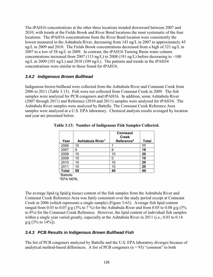
126

The tPAH16 concentrations at the other three locations trended downward between 2007 and 2010, with trends at the Fields Brook and River Bend locations the most systematic of the four locations. The tPAH16 concentrations from the River Bend location were consistently the lowest measured in the Ashtabula River, decreasing from 143 ng/L in 2007 to approximately 45 ng/L in 2009 and 2010. The Fields Brook concentrations decreased from a high of 321 ng/L in 2007 to a low of 58 ng/L in 2009. In contrast, the tPAH16 Turning Basin water column concentrations increased from 2007 (113 ng/L) to 2008 (191 ng/L) before decreasing to ~100 ng/L in 2009 (101 ng/L) and 2010 (109 ng/L). The patterns and trends in the tPAH34 concentrations were similar to those found for tPAH16.

3.4.2 Indigenous Brown Bullhead

Indigenous brown bullhead were collected from the Ashtabula River and Conneaut Creek from 2006 to 2011 (Table 3.13). Fish were not collected from Conneaut Creek in 2009. The fish samples were analyzed for PCB congeners and tPAH16. In addition, some Ashtabula River (2007 through 2011) and Reference (2010 and 2011) samples were analyzed for tPAH34. The Ashtabula River samples were analyzed by Battelle. The Conneaut Creek Reference Area samples were analyzed at a U.S. EPA laboratory. Chemical analysis results averaged by location and year are presented below.

Table 3.13: Number of Indigenous Fish Samples Collected.

Year Ashtabula River1

Conneaut Creek

Reference2 Total 2006 10 1 11 2007 9 9 18 2008 10 10 20 2009 10 0 10 2010 10 10 20 2011 10 10 20 Total 59 40 99

1Battelle 2EPA NERL

The average lipid (g lipid/g tissue) content of the fish samples from the Ashtabula River and Conneaut Creek Reference Area was fairly consistent over the study period except at Conneaut Creek in 2006 (which represents a single sample) (Figure 3-63). Average fish lipid content ranged from 0.03 to 0.07 g/g (3% to 7 %) for the Ashtabula River and from 0.05 to 0.08 g/g (5% to 8%) for the Conneaut Creek Reference. However, the lipid content of individual fish samples within a single year varied greatly, especially at the Ashtabula River in 2011 (i.e., 0.03 to 0.14 g/g [3% to 14%]). 3.4.3 PCB Results in Indigenous Brown Bullhead Fish

The list of PCB congeners analyzed by Battelle and the U.S. EPA laboratory diverges because of analytical method-based differences. A list of PCB congeners (n = 93) “common” to both

127

laboratories’ analyses was developed as a way to present and compare tPCB(c) results between the two locations. Summary tables of results for tPCB(c) and percent lipids are provided in Appendix G.

Note: n=10 for all years except 2007 (n=9), 2006 Conneaut Creek Reference (n=1), and 2009 Conneaut Creek Reference (n=0)

Figure 3-63. Average Lipid Content with Error Estimates (Standard Deviations) in Indigenous Brown Bullhead Collected from the Ashtabula River and Conneaut Creek.

The wet weight tPCB(c) concentration in brown bullhead from the Ashtabula River varied similarly whether aggregated as the full PCB congener list or the “common” PCB congener list (Figure 3-64; A). Moreover, the Conneaut Creek PCBs were significantly less than the Ashtabula River samples regardless of aggregation method.

Temporally, the by-weight tPCB(c) concentrations in the brown bullheads peaked in 2007 (4.754 mg/kg wet wt) when remedial dredging was active. This 2007 peak was followed by decreasing concentrations through 2009 (0.965 mg/kg wet wt). tPCB(c) concentrations increased in 2010 and 2011 (an average of 1.44 mg/kg wet wt), a value that is approximately 50% higher than the 2009 low. The PCB concentrations in the brown bullhead from the Conneaut Creek Reference ranged from 0.110 to 0.262 mg/kg wet wt from 2006 to 2011.

Lipid normalization changed the temporal pattern in the Ashtabula River, specifically the tPCB(c) maximum concentration shifted from 2007 to 2008 (108 mg/kg lipid), although uncertainty in the means measured as the standard deviation of the average suggest the shift was

128

not significant (Figure 3-64; B). However, the 2009 minimum was consistent with un-normalized results and was followed by a slight increase in 2010 and 2011 (39 mg/kg lipid). The Conneaut Creek Reference brown bullhead lipid-normalized concentrations were low and consistent with un-normalized PCB data, with the highest measured concentration occurring in 2006 (14.6 mg/kg lipid) and the lowest in 2011 (2.3 mg/kg lipid).

The brown bullhead PCB data from the Ashtabula River were dominated by tetra, penta, hexa, and hepta homologs in all years (Figure 3-65). The relative homolog contributions were strikingly consistent across the study period. In contrast, the Conneaut Creek Reference fish had high relative concentrations of the di homolog in 2006, but hexa homologs were more prevalent and relatively consistent in the 2007 through 2011 samples. These variations in the homolog distribution in the Conneaut Creek Reference samples appears to be due to low concentrations near the MDL that skew the composition distribution. The Ashtabula River samples also appear to have a greater contribution of hepta homolog series than measured in the Conneaut Creek Reference samples, clearly supporting different PCB source types. 3.4.4 PAH Results in Indigenous Brown Bullhead Fish

tPAH16 concentrations in the brown bullhead catfish were elevated in 2006 and 2007 (0.191 and 0.196 mg/kg wet wt, respectively), with decreased concentrations in 2008 through 2011 (ranging from 0.056 to 0.111 mg/kg wet wt) (Figure 3-66). In contrast, the Conneaut Creek tPAH16 concentrations increased notably from 2006 to 2007. The apparently elevated 2007 concentrations decreased from 0.111 to 0.047 mg/kg wet wt. between 2008 and 2011. The trends in the lipid-normalized tPAH16 concentrations in the Ashtabula River samples were similar to those in the un-normalized data. The elevated concentrations in the Ashtabula River samples in 2006 (4.9 mg/kg lipid) and 2007 (3.1 mg/kg lipid) decreased to 1.3 to 1.8 mg/kg lipid in the 2008 through 2010 period. In contrast to the un-normalized concentrations, the lipid-normalized concentrations increased in 2011 (3.0 mg/kg lipid) to concentrations similar to those measured in 2007. The lipid-normalized tPAH16 concentrations in brown bullhead catfish from the Conneaut Creek Reference (0.6 to 2.2 mg/kg lipid) were generally lower than or similar to catfish from Ashtabula River. tPAH34 concentrations were not available for catfish collected from the Ashtabula River in 2006. The highest concentrations measured were in 2007 (0.710 mg/kg wet wt.). tPAH34 concentrations were substantially lower and relatively consistent between 2008 and 2011 (ranging from 0.106 to 0.192 mg/kg wet wt). These concentrations were similar to those in catfish collected from the Conneaut Creek Reference in 2010 and 2011 (0.152 and 0.083 mg/kg wet wt, respectively). The lipid-normalized tPAH34 data trend (Figure 3-66) was similar to the un-normalized results, although slightly more variable. The highest lipid normalized tPAH34 lipid concentration was reported for 2007 (11.2 mg/kg lipid) and ranged from 3 to 4.6 mg/kg lipid from 2008 to 2011. The 2010 and 2011 Conneaut Creek Reference lipid-normalized tPAH34 concentrations (2.51 and 1.14 mg/kg lipid, respectively) were similar, possibly lower than those for the Ashtabula River.

129

Note: n=10 for all years except 2007 (n=9) and 2006 Conneaut Creek Reference (n=1) and 2009 Conneaut Creek Reference (n=0)

Figure 3-64. tPCB(c) Concentrations (mg/kg wet wt [A], and mg/kg lipid-normalized [B]) with Error Estimates (Standard Deviations) in Indigenous Brown Bullhead Collected from the Ashtabula River and Conneaut Creek.

130

2006 is Pre-Dredge; 2007 is During Dredge; 2008 – 2011 are Post-Dredge. Note: No fish were collected from the Conneaut Creek Reference in 2009. Figure 3-65. Percent of tPCB(c) as Homolog Contributions in Brown Bullhead Collected from the (A) Ashtabula River and

(B) Conneaut Creek Reference (2006-2011).

A B

131

*Total tPAH34 concentrations were not available for fish from Ashtabula River in 2006.

Figure 3-66. tPAH16 (wet wt [A] and Lipid-Normalized [B]); and tPAH34 (wet wt [C] and Lipid-Normalized [D]) Concentrations in Indigenous Brown Bullhead with Error Estimates (Standard Deviation) Collected from the Ashtabula River and Conneaut Creek

Reference (2006-2001).

132

3.5 Passive Samplers as Biological Surrogates Hydrophobic chemicals, such as PCBs, are known to accumulate in lipophilic materials. This principle is the basis for the design of most passive samplers for organic chemicals. Two common passive samplers use solid phase microextraction (SPME) and semipermeable membrane device (SPMD) materials to measure organics in water, porewater, and sediments. It is well established that when the chemical nature and partitioning coefficients of these materials are known, the hydrophobic chemical concentration measured in the passive sampler can be used to calculate the time-weighted chemical concentration in the water in which the sampler is placed. This assumes the chemical has attained equilibrium between the materials and water that is sampled. The addition of performance reference compounds (PRCs) allows for estimation of uptake even if equilibrium is not reached. The advantage in using these samplers compared to analyzing water and sediment samples directly is that the concentration of contaminants in the passive samplers represents a time-weighted average. Compared to collecting and analyzing biological samples (e.g., indigenous fish), passive samplers provide sampling at a fixed location and are easier to deploy and retrieve than collecting biological samples.

SPMDs (EST, St. Joseph, MO) were deployed at a series of water column locations in the Ashtabula River in 2006, 2008, and 2011 (Figure 2-5 and Table 2.5). These locations are primarily in the river reach that was remediated in 2006/2007. Perforated stainless steel carrier canisters that housed the water column SPMDs were attached to a buoy that suspended the SPMDs approximately 1 m above the sediment surface for 28 days (U.S. EPA, 2011b). Five SPMDs were deployed at each site and after recovery were composited at the laboratory for chemical analysis. Duplicate sediment SPMD samples were recovered for chemical analysis from Stations 3, 4, and 6 in 2006, from Stations 1, 3, 4, and 5 in 2008, and from Stations 23 and 24 in 2011 (see Table 2.5). Single samples were available from the remaining locations. Those stations with duplicates were averaged together, and the tPCB(c) concentration was used in analysis and graphing. For sediment, five SPMDs were deployed in specially designed racks at a series of locations in the Ashtabula River (Figure 2-4; U.S. EPA, 2011b). These SPMDs were also deployed for 28 days. Each SPMD was lightly rinsed using site water on recovery to remove excess sediment that adhered to the sampler. All five SPDMs from a location were transferred into a common hexane-rinsed can for shipment to the laboratory. The five SPMDs from each site were composited at the laboratory for chemical analysis. The results from each matrix, as well as from co-located water and sediment samples, were evaluated (U.S. EPA, 2006, 2007, 2011a). The south-to-north (upriver-to-down river) geospatial relationship shown in Figures 2-4 and 2-5 was retained among the locations presented in the figures. SPMD data were reported on the basis of individual SPMDs, which enabled the SPMD data to be converted to water equivalent data using published USGS spreadsheet conversion models (Alvarez, 2010a; Alvarez, 2010b): The data presentation that follows is separated into subsections that summarize the SPMD water, SPMD sediment, SPME water, and SPME sediment results. Summary tables of tPCB(c) and tPCB(H) for co-located sediments and waters are provided in Appendix H.

133

3.5.1 Water Column SPMDs

Water column SPMDs were deployed in the Ashtabula River at up to 11 stations in 2006, 2008, and 2011 (Table 3.14 and Table 2.5). One SPMD composite sample was collected per station, except at Stations 23 and 24 in 2011, where duplicate composite samples were collected at these two stations. Co-located whole (not filtered) water samples were also collected at most locations, with one field duplicate sample collected in each sampling year. The SPMD PCB data are evaluated in terms of two concentration units: 1) mass of chemical per SPMD (SPMD volumes are uniform across the individual samplers); and 2) converted to equivalent water column concentrations (pg/L). Two approaches for the conversion were used; one was PRC-corrected, and the other was uncorrected. The conversions were accomplished with published USGS spreadsheet models: Version 4.1 - Estimated Water Concentration Calculator from SPMD Data When Not Using PRCs (Alvarez, 2010b) and USGS spreadsheet Version 5.1 - Estimated Water Concentration Calculator from SPMD Data Using PRCs (Alvarez, 2010a). The conversion process for SPMD data spiked with PRCs used the following equation:

𝐶𝑤=

𝑁

(𝑉𝑠𝐾𝑠𝑤[1−𝑒𝑥𝑝(−𝑅𝑠𝑡𝑉𝑠𝐾𝑠𝑤

)])

(Equation 3-17)

where N = the amount of chemical accumulated by the sample (typically in ng); Vs = volume of the SPMD (in L or ml); Ksw = SPMD-water partition coefficient Rs = the sampling rate (L/d); and t = the exposure time (d). Regression models are used to estimate a chemical’s site specific sampling rate (Rs) and SPMD-water partition coefficient (Ksw) using the chemical’s partitioning coefficient, loss rate of the PRC from the SPMD during deployment, and the volume of the SPMD (Huckins et al., 2006). The conversion process for SPMD data without added PRCs utilizes the same equation, but experimentally-derived Rs values are used instead of a site-specific sampling rate calculated when PRCs are added (Alvarez, 2001c). Alvarez (2010c) contains additional guidance regarding the use of these equations and provides the experimentally derived R values.

Table 3.14: Number of Water Column SPMDs and Co-located Water Samples Collected.

Year Water Column SPMDs

Co-located Water Samples

2006 11 10 2008 10 12 2011 13 12

In cases where PCB data were reported as ng/SAMPLE, the data were first converted to ng/SPMD by dividing by the number of SPMDs in each composited sample (generally five

134

SPMDs aggregated into one analytical sample). An average volume from the five composite SPMDs was used as the SPMD volume for each analytical sample. Where measurements were not available for specific SPMDs, an average volume of all the SPMDs deployed in that year was used. Where available, SPMD dimensions and weights were used to estimate the SPMD volume required for the water column concentration conversion.

The available PRCs varied depending on the survey year: 2006 – PCB 38 and PCB 50

2008 – PCB 29, PCB 38, PCB 50, PCB 166

2011 – PCB 38 and PCB 186 (note: PCB 186 could not be used in the conversion calculation because final mass was greater than initial mass for most SPMD samples).

3.5.1.1 PCB Trends in Water Column SPMD Concentrations

PCB concentrations per SPMD were comparatively similar across all stations within a given year (Figure 3-67). The concentrations appeared most variable in 2006 and least variable (most similar) in 2011. Water column PCB concentrations (ng/SPMD) measured by the SPMDs decreased at five stations (15, 3, 25, 24, and 22) after the 2006/2007 dredging. Five other stations (1, 4, 23, 8, and 5) showed slight increases from 2006 to 2008. The stations that decreased were generally located in the dredged upriver reach (except for Station 22, which was located just downstream of the area dredged); those that increased were in the dredged down-river reach (except for Station 1 located in the Upstream area and Station 4 in the middle of the area dredged). Every station appeared to have lower SPMD concentrations in 2011 compared to 2008, but with variable degrees of relative decrease.

The PCB concentrations of water samples collected within each year were similar across all stations but changed dramatically after 2006. Specifically, the PCB concentrations decreased about five-fold between 2006 and 2008. In contrast, PCB concentrations in the 2008 and 2011 water samples were similar (Figure 3-68), although 2011 concentrations were slightly lower than in 2008.

An important consideration is the comparison of water sample COC concentrations with water column SPMD COC concentrations. This comparison was accomplished by converting the SPMD data to water concentration equivalent data. Figure 3-69 compares the 2006 PRC- and non-PRC-corrected SPMD concentrations to the co-located water concentrations. Major concentration differences are evident among the three approaches. Most glaring is the large difference between the measured and calculated water concentrations. Specifically, the 2006 PRC-corrected PCB concentrations determined from the water column SPMDs are up to 20 times lower than the measured water column concentration (~100 ng/L), while the uncorrected data are five to 10 times lower. However, it is important to note that the measured total PCBs in the water column include both dissolved and particulate fractions, while the SPMD data reflect only the “dissolved” or mobile PCB fraction. This artifact of the measurement likely accounts for the elevated tPCB(c) concentrations observed in the co-located water samples compared to the true ‘dissolved’ concentrations measured by the SPMDs. TSS concentrations (mg/L)

135

measured in the co-located water samples in 2006 indicate that the water column concentrations of tPCB(c) were likely elevated due to inclusion of the particulate bound PCBs present (Figure 3-69). Overall trends in concentrations between SPMD PCBs and water column PCBs were similar.

*Note: No water column SPMD was collected at Station 12 during retrieval. Average of duplicate samples at Stations 3, 4, and 6 in 2006; from Stations 1, 3, 4, and 5 in 2008; and from Stations 23 and 24 in 2011.

Figure 3-67. tPCB(c) Concentration per SPMD Suspended in the Water Column. Contrary to the above observations, the 2008 and 2011 PCB concentrations in the water samples were fairly similar to the equivalent water column concentrations calculated from the water column SPMDs (Figures 3-70 and 3-71). More specifically, the measured PCBs were approximately five times lower in both 2008 and 2011 than in 2006, and the PRC- and non-PRC-corrected SPMD concentrations were on the order of two to four times less than the measured concentrations. TSS concentrations were also two to five times lower in 2008 and 2011 compared to 2006. The relative order of concentrations among the three approaches did not change among the 3 years (measured concentrations highest, followed by uncorrected equivalent concentrations, followed by PCR-corrected equivalent concentrations as the lowest) although the relative separation between the PRC- and non-PRC-corrected SPMD data appears to decrease between 2008 and 2011. Moreover, less spatial variability is apparent among the stations in 2008 and 2011 (for both co-located water and equivalent water) relative to 2006.

136

*Note: No water samples were collected at Station 1 and Station 25 in 2006.

Figure 3-68. tPCB(c) Concentrations in Co-located Whole Water Samples. An additional comparison that the experimental design enabled was the ability to contrast temporal responses for spatially averaged annual concentrations. Notably, the PRC-corrected equivalent PCB concentrations (Figure 3-72) averaged across all sampling stations by year did not reveal a clear temporal trend from 2006 to 2011. The non-PRC-corrected PCB concentrations may have decreased slightly in 2011 relative to 2006 and 2008. In contrast, the average water sample PCB and TSS concentrations markedly decreased from 2006 to 2008; a further slight decrease in PCB concentrations appears between 2008 and 2011. However, it is important to note, as described above, that the measured total PCBs in the water column include both dissolved and particulate fractions, while the SPMD data reflect only the “dissolved” PCB fraction. The TSS data indicate that the particulates in the whole water samples used for this comparison are greatly influencing the total PCB concentrations in the water samples. Hence, future comparison of water column and passive sampler data must ensure that the particulate fraction is removed from the sample before extraction.

137

Figure 3-69. 2006 PRC- and Non-PRC-corrected Water Column SPMD tPCB(c) Concentrations Compared to Co-located Whole Water tPCB(c) and TSS Concentrations.

Note: No water column SPMDs were collected at Station 12 during retrieval.


138


Figure 3-72. Inter-annual Comparison of tPCB(c) Concentrations (Average and Standard Deviation of 11 Stations in 2006 and 2011; 10 stations in 2008) for PRC- and

Non-PRC-corrected Water Column SPMDs to Whole Water Concentrations.

139

3.5.1.2 PCB Distribution in the Water Column SPMDs and Co-located Water Samples

The spatially averaged PCB distributions in the SPMD samples were comprised mainly of tetra, tri, and penta homolog groups (Figure 3-73). Little change in the distribution of the homolog groups measured in the water SPMDs was noted over time, except for a slight decrease in the percentage of hexa and hepta homolog groups from 2006 to 2008 (and an associated increase in tetra and tri homolog groups). The 2008 and 2011 PCB homolog distributions were very similar. PCB homolog distribution in the whole water samples (Figure 3-73) was substantially different than found in the SPMD samples. The 2006 water column PCB distribution consisted mainly of heavier homologs, including hexa, penta, and octa homolog groups (Figure 3-73). Moreover, there was a shift in the distribution between 2006 and 2008 with the lighter homologs making up a larger percentage of tPCB(c)s in 2008. Specifically, the percentage of octa and nona homologs decreased in 2008, whereas the percentages of tri and tetra homologs increased. There was little change in the percentages of homolog groups between the 2008 and 2011 water samples. The comparability of the homolog distribution in the measured and SPMD samples may be biased by the inclusion of organic particulates in the whole water samples. As mentioned earlier, it is important to understand the role of the particulate fraction when comparing PCB concentrations in SPMD samples with those in whole water samples as the SPMDs measure only the dissolved fraction. Also, the SPMDs provide data as a time-weighted average concentration of a chemical within the whole exposure period, which may account for some of the differences seen in the PCB distribution of the two sampling methods.

140

Figure 3-73. Percent of tPCB(c) as Homolog Distributions for (A) Water Column SPMD Samples and (B) Co-located Water Column Samples from the Ashtabula River (2006, 2008, and 2011).

A B

141

3.5.2 Sediment SPMDs

Sediment SPMDs were deployed on the sediment surface in the Ashtabula River at 24, 22, and 11 stations in 2006, 2008, and 2011, respectively (U.S. EPA, 2006, 2007, 2011). One SPMD composite sample was collected per station (Table 3.15), except at Stations 1, 3, 4, and 5 in 2008 and Stations 23 and 24 in 2010, where duplicate composite samples were collected at these stations. Co-located sediment samples were also collected at 10 or 11 of these locations, with one field duplicate sample collected in 2008 and 2010.

The sediment SPMD data were reported as ng/SAMPLE. Consistent with the water column SPMD data, these concentrations were converted to ng/SPMD by dividing the sample concentration by the number of SPMDs in each sample (five SPMDs per sample). The PCB concentrations in the sediment SPMDs varied spatially in each of the 3 years they were deployed (Figure 3-74). The sediment SPMD PCB concentrations also appeared to be more variable in 2006 than in subsequent years. The highest sediment SPMD PCB concentrations were measured during the pre-dredge sampling of 2006 (Figure 3-74). The only exception was at Station 1, where the 2011 Total PCB concentrations were higher than in 2006 and 2008. The PCB concentrations in the co-located sediment samples were typically less than 600 ng/g dry wt and similar across stations and years (within a factor of two). Exceptions to this were at Stations 1 and 24 in 2011, where concentrations of tPCB(c)s were greater than at any other station or sampling year (Figure 3-75). The average PCB concentrations in sediment SPMDs decreased from 1,622 ng/SPMD in 2006 to 564 ng/SPMD in 2008 (~65% decrease). Comparatively, the average PCBs in the co-located sediment samples decreased by ~12% (0.433 mg/kg dry in 2006 vs. 0.381 mg/kg dry in 2008) (Figure 3-76). The PCB concentrations in both sediment SPMDs and co-located sediment samples increased from 2008 to 2011 (581 ng/SPMD and 0.621 mg/kg dry). This increase observed in 2011 may have been due to individual samples that had PCB concentrations notably greater than at other stations (i.e., sediment SPMD at Station 25 [Figure 3- 74] and co-located sediment at Stations 1 and 24 [Figure 3-75]). Some of these locations (Stations 24 and 25) were not sampled prior to 2011 and were not included in the 2008 dataset.

Table 3.15: Number of Sediment SPMDs and Co-located Sediment Samples Collected.

Year Sediment SPMDs

Co-located Sediment Samples

2006 24 10 2008 26 12 2010 13 12

142

3.5.2.1 PCB Distribution in Sediment SPMDs and Co-located Sediment Samples

PCBs in sediment SPMDs were comprised mainly of tri, tetra, and penta homolog groups, with very little presence of nona or deca homologs (Figure 3-77). Little change was in the homolog groups measured in the sediment SPMDs over time, except for a decrease in the percentage of hexa through nona homolog groups from pre-dredge 2006 to post-dredge 2008. The percentage of hexa homologs increased in post-dredge 2011, while the tetra homolog percentage decreased. PCBs in co-located sediment samples also consisted of mainly tri, tetra, and penta homolog groups, but with a larger contribution of heavier congeners (hepta through deca homolog groups) (Figure 3-77). From pre-dredge 2006 to post-dredge 2008, the percentage of tetra homologs in co-located sediments increased, while the percentage of hexa, hepta, and octa homolog groups decreased. There was little change in the percentages of homolog groups between post-dredge 2008 and post-dredge 2011 in co-located sediment. Overall, the spatial distribution of PCBs in sediment SPMDs and co-located sediments was similar over time.

*Note: No sediment SPMDs were deployed at Stations 2, 20, 16, 14, 13, 18, 11, 19, 10, 21, 9, 17, 7, 6 in 2011; none at Stations 25, 24, 23 in 2006 and 2008; and none at Station 22 in 2006.

Figure 3-74. tPCB(c) Concentration per SPMD Placed on Surface Sediments from the

Ashtabula River (2006 [n=21], 2008 [n=22], and 2011 [n=11]).

143

Figure 3-75. tPCB(c) Concentrations in Ashtabula River Surface Sediment Samples Co-located with Sediment SPMDs (2006 [n=6], 2008 [n=8], and 2011 [n=11]).

Figure 3-76. Comparison of Average tPCB(c) Concentrations in Ashtabula River Sediment SPMDs and Co-located Sediment Samples (2006 [n=7], 2008[n=8], and

2011[n=11]).

0.0

0.5

1.0

1.5

2.0

2.5

3.0

3.5

STA

TIO

N 2

STA

TIO

N 1

STA

TIO

N 2

0

STA

TIO

N 1

6

STA

TIO

N 1

5

STA

TIO

N 3

STA

TIO

N 1

4

STA

TIO

N 2

5

STA

TIO

N 1

3

STA

TIO

N 1

8

STA

TIO

N 1

2

STA

TIO

N 1

1

STA

TIO

N 1

9

STA

TIO

N 4

STA

TIO

N 1

0

STA

TIO

N 2

4

STA

TIO

N 2

1

STA

TIO

N 9

STA

TIO

N 2

3

STA

TIO

N 8

STA

TIO

N 1

7

STA

TIO

N 7

STA

TIO

N 6

STA

TIO

N 5

STA

TIO

N 2

2

tPC

B(

c) (

mg

/kg

dry

)

Upstream to Downstream

PRE-DREDGE 2006

POST-DREDGE 2008

POST-DREDGE 2011

0.0

0.5

1.0

1.5

2.0

2.5

3.0

PRE-DREDGE 2006

DURING-DREDGE 2007

POST-DREDGE 2008

POST-DREDGE 2009

POST-DREDGE 2010

POST-DREDGE 2011

Ave

rage

tPC

B(

c) (

mg

/SP

MD

or

mg

/kg

dry

)

Sediment SPMD

Co-located Sediment

144

3.5.2.2 Estimation of Porewater Concentrations from Sediment SPMDs

The bioavailability of chemicals in sediments is often estimated using their concentrations in sediment porewater. The sediment SPMD PCB data were converted to equivalent porewater concentrations (pg/L) using the same models as those applied to the water column SPMDs (Section 3.5.1). Two approaches for the conversion were employed: 1) PRC-corrected, and 2) uncorrected. The conversions were accomplished with published USGS spreadsheet models: Version 4.1 - Estimated Water Concentration Calculator from SPMD Data When Not Using PRCs (Alvarez, 2010b) and USGS spreadsheet Version 5.1 - Estimated Water Concentration Calculator from SPMD Data Using PRCs (Alvarez, 2010a). The conversion process is summarized below. In cases where PCB data were reported in the database as ng/sample, the data were first converted to ng/SPMD by dividing by the number of SPMDs in each composited sample (five SPMDs were aggregated into one analytical sample). An average volume from the five composite SPMDs was used as the SPMD volume for each analytical sample. Where measurements were not available for specific SPMDs, an average volume of all the SPMDs deployed in that year was used. Where available, SPMD dimensions and weights were utilized to estimate the SPMD volume required for the porewater concentration conversion. The available PRCs ranged from one to four, depending on the survey year:

2006 – PCB 38 and PCB 50 2008 – PCB 29, PCB 38, PCB 50, and PCB 166 2011 – PCB 38 and PCB 186

For some SPMDs in 2006, the PRCs could not be used in the conversion calculation because the final mass of the PRC was greater than the initial mass. The stations affected in 2006 were the following:

Stations 1, 10, 11, 13, 16, 18, 19, 2, 20, 3, 4 (both duplicates), 6 (both duplicates), 9

A comparison was made of the estimated porewater concentrations of PCBs to those in the overlying water column (~30 cm from the water-sediment interface). Porewater concentrations and surface waters represent different environmental compartments. It is often beneficial to compare those data to determine potential flux into or out of the sediment. Figure 3-78A compares the 2006 PRC- and non-PRC-corrected SPMD concentrations to the co-located water concentrations. Major concentration differences are evident among the three approaches. The co-located water concentrations were much higher than those estimated using the SPMDs deployed at the sediment surface for all years. Specifically, the 2006 PRC-corrected tPCB(c) concentrations calculated from SPMD data, were more than 20 times lower than the measured concentration in the co-located water samples, while the uncorrected data is five to 10 times lower. However, as described previously (Section 3.5.1.1), the measured tPCB(c) in the water column include both dissolved and particulate fractions, while the SPMD data reflect only the “dissolved” PCB fraction. TSS concentrations (mg/L) measured in the co-located water samples

145

Figure 3-77. Percent of tPCB(c) as Homolog Distributions for (A) SPMDs Placed on Surface Sediments, and (B) Co-located Sediment Samples from the Ashtabula River (2006, 2008, and 2011).

A B

146

in 2006 indicate that the water column concentration of tPCB(c) was likely elevated due to inclusion of the particulate-bound PCBs present (Figure 3-69). In contrast, the 2008 and 2011 tPCB(c) concentrations in the water samples were more similar to the equivalent porewater column concentrations calculated from the sediment SPMDs (Figures 3-78B and 3-78C). More specifically, the measured tPCB(c)s were approximately five times lower in both 2008 and 2011 than in 2006 and the PRC- and non-PRC-corrected SPMD concentrations were approximately two times less than the 2006 concentrations. The relative separation between the PRC- and non-PRC-corrected SPMD data appears to decrease from 2006 to 2011 for most stations. Overall, no evident trends were apparent in concentrations across stations for either the SPMD or measured water concentrations for any year; however, there appears to be less spatial variability among the stations in 2008 and 2011 (for both co-located water and equivalent porewater) relative to 2006.

An additional comparison enabled by the experimental design was the ability to contrast temporal responses for spatially-averaged annual concentrations. The PRC-corrected and non-corrected equivalent PCB concentrations (Figure 3-79) averaged across all sampling stations by year revealed a notable decrease in tPCB(c) concentrations from 2006 to 2008, with a slight subsequent increase in 2011.

147

Note: A = 2006; B = 2008; C = 2011

Figure 3-78. Estimated Porewater Concentrations (PRC- and Non-PRC-corrected) Compared to Co-located Water Concentrations for 2006, 2008, and 2011.

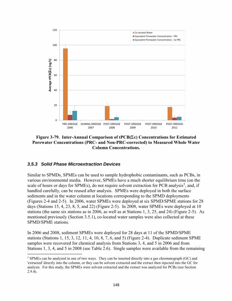
148

Figure 3-79. Inter-Annual Comparison of tPCB(c) Concentrations for Estimated Porewater Concentrations (PRC- and Non-PRC-corrected) to Measured Whole Water

Column Concentrations. 3.5.3 Solid Phase Microextraction Devices

Similar to SPMDs, SPMEs can be used to sample hydrophobic contaminants, such as PCBs, in various environmental media. However, SPMEs have a much shorter equilibrium time (on the scale of hours or days for SPMEs), do not require solvent extraction for PCB analysis 6F

5, and, if handled carefully, can be reused after analysis. SPMEs were deployed in both the surface sediments and in the water column at locations corresponding to the SPMD deployments (Figures 2-4 and 2-5). In 2006, water SPMEs were deployed at six SPMD/SPME stations for 28 days (Stations 15, 4, 23, 8, 5, and 22) (Figure 2-5). In 2008, water SPMEs were deployed at 10 stations (the same six stations as in 2006, as well as at Stations 1, 3, 25, and 24) (Figure 2-5). As mentioned previously (Section 3.5.1), co-located water samples were also collected at these SPMD/SPME stations. In 2006 and 2008, sediment SPMEs were deployed for 28 days at 11 of the SPMD/SPME stations (Stations 1, 15, 3, 12, 11, 4, 10, 8, 7, 6, and 5) (Figure 2-4). Duplicate sediment SPME samples were recovered for chemical analysis from Stations 3, 4, and 5 in 2006 and from Stations 1, 3, 4, and 5 in 2008 (see Table 2.6). Single samples were available from the remaining 5 SPMEs can be analyzed in one of two ways. They can be inserted directly into a gas chromatograph (GC) and 'extracted' directly into the column, or they can be solvent extracted and the extract then injected into the GC for analysis. For this study, the SPMEs were solvent extracted and the extract was analyzed for PCBs (see Section 2.9.4).

0

20

40

60

80

100

120

PRE-DREDGE2006

DURING-DREDGE2007

POST-DREDGE2008

POST-DREDGE2009

POST-DREDGE2010

POST-DREDGE2011

Ave

rage

tP

CB

(c)

(ng

/L)

Co-located Water

Equivalent Porewater Concentration - PRC

Equivalent Porewater Concentration - no PRC

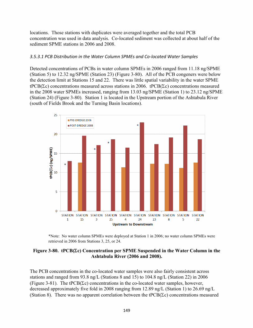
149

locations. Those stations with duplicates were averaged together and the total PCB concentration was used in data analysis. Co-located sediment was collected at about half of the sediment SPME stations in 2006 and 2008. 3.5.3.1 PCB Distribution in the Water Column SPMEs and Co-located Water Samples

Detected concentrations of PCBs in water column SPMEs in 2006 ranged from 11.18 ng/SPME (Station 5) to 12.32 ng/SPME (Station 23) (Figure 3-80). All of the PCB congeners were below the detection limit at Stations 15 and 22. There was little spatial variability in the water SPME tPCB(c) concentrations measured across stations in 2006. tPCB(c) concentrations measured in the 2008 water SPMEs increased, ranging from 13.03 ng/SPME (Station 1) to 23.12 ng/SPME (Station 24) (Figure 3-80). Station 1 is located in the Upstream portion of the Ashtabula River (south of Fields Brook and the Turning Basin locations).

*Note: No water column SPMEs were deployed at Station 1 in 2006; no water column SPMEs were retrieved in 2006 from Stations 3, 25, or 24.

Figure 3-80. tPCB(c) Concentration per SPME Suspended in the Water Column in the Ashtabula River (2006 and 2008).

The PCB concentrations in the co-located water samples were also fairly consistent across stations and ranged from 93.8 ng/L (Stations 8 and 15) to 104.8 ng/L (Station 22) in 2006 (Figure 3-81). The tPCB(c) concentrations in the co-located water samples, however, decreased approximately five fold in 2008 ranging from 12.89 ng/L (Station 1) to 26.69 ng/L (Station 8). There was no apparent correlation between the tPCB(c) concentrations measured

150

with the SPMEs and the concentrations in the co-located water samples; water concentrations decreased substantially from 2006 to 2008, while SPME concentrations exhibited a marginal increase over the same time period. As mentioned earlier, TSS concentrations (mg/L) measured in the co-located water samples in 2006 indicated that the water column concentration of tPCB(c) was likely elevated due to inclusion of the particulate-bound PCBs present (Figure 3-69).

The spatially-averaged PCB distribution in the SPME samples was comprised mainly of tetra, penta, and hexa homolog groups (Figure 3-82A). The percentage of tetra and tri homolog groups increased from 2006 to 2008, while an associated decrease occurred in the penta and hexa homolog groups.

Comparatively, tPCB(c) homolog distribution in the water samples was somewhat different than found in the SPME samples (Figures 3-82 B and 3-82A, respectively). The 2006 water column PCB distribution consisted mainly of heavier homologs, including hexa, penta, and octa homolog groups (Figure 3-82B). Moreover, there was a shift in the distribution between 2006 and 2008, with the lighter homologs making up a larger percentage of tPCB(c)s in 2008. Specifically, the percentage of octa and nona homologs decreased in 2008, whereas the percentages of tri and tetra homologs increased. Therefore, the PCB distribution in water samples in 2008 became more similar to the distribution in the SPME samples.

Figure 3-81. tPCB(c) Concentrations in Water Samples Co-located with SPMEs in the Ashtabula River (2006 and 2008).

0

20

40

60

80

100

120

STATION1

STATION 15

STATION3

STATION 25

STATION4

STATION 24

STATION 23

STATION8

STATION5

STATION 22

tPC

B(

c)(n

g/L

)


PRE-DREDGE 2006

POST-DREDGE 2008

151

3.5.3.2 PCB Distribution in the Sediment SPMEs and Co-located Sediment Samples

Detected tPCB(c) concentrations in sediment SPMEs ranged from 10.98 ng/SPME (Station 3) to 12.43 ng/SPME (Station 7) in 2006 (Figure 3-83). All of the PCB congeners were below the detection limit at Station 1 in both 2006 and 2008 (1/2 the detection limit was used to calculate the tPCB(c) concentrations for this station). tPCB(c) concentrations measured in the sediment SPMEs were greater and more variable in 2008, ranging from 13.2 ng/SPME (Station 7) to 19.72 ng/SPME (Station 12). Most PCB congeners in the sediment SPME samples were not detected. Most of the congeners detected were either tetrachlorobiphenyls, trichlorobiphenyls, or pentachlorobiphenyls, with more detections occurring in 2008 than in 2006. tPCB(c) concentrations in the co-located sediment (top 10 cm) collected from six SPME stations in 2006 ranged from 0.152 mg/kg dry wt (Station 3) to 0.563 mg/kg dry wt (Station 12) (Figure 3-84). Co-located sediment was collected at seven of the SPME stations in 2008. tPCB concentrations in the co-located sediment ranged from 0.043 mg/kg dry wt (Station 1) to 0.533 mg/kg dry wt (Station 5). There was no apparent correlation between the tPCB concentrations measured with the SPMEs and the concentrations in the co-located sediment; tPCB concentrations in surface sediments increased at some SPME stations from 2006 to 2008 and decreased at other stations.

Comparatively, tPCB(c) homolog distribution measured in the sediment samples (Figure 3-82C and 3-82D) was somewhat different than found in the SPME samples. The 2006 sediment PCB distribution consisted mainly of tetra, penta, and tri homolog groups. Moreover, a shift occurred in the distribution between 2006 and 2008, with the lighter homologs making up a majority of tPCB(c) in 2008. Specifically, the percentage of penta, hexa, and octa homologs decreased in 2008, whereas the percentages of tri and tetra homologs increased.

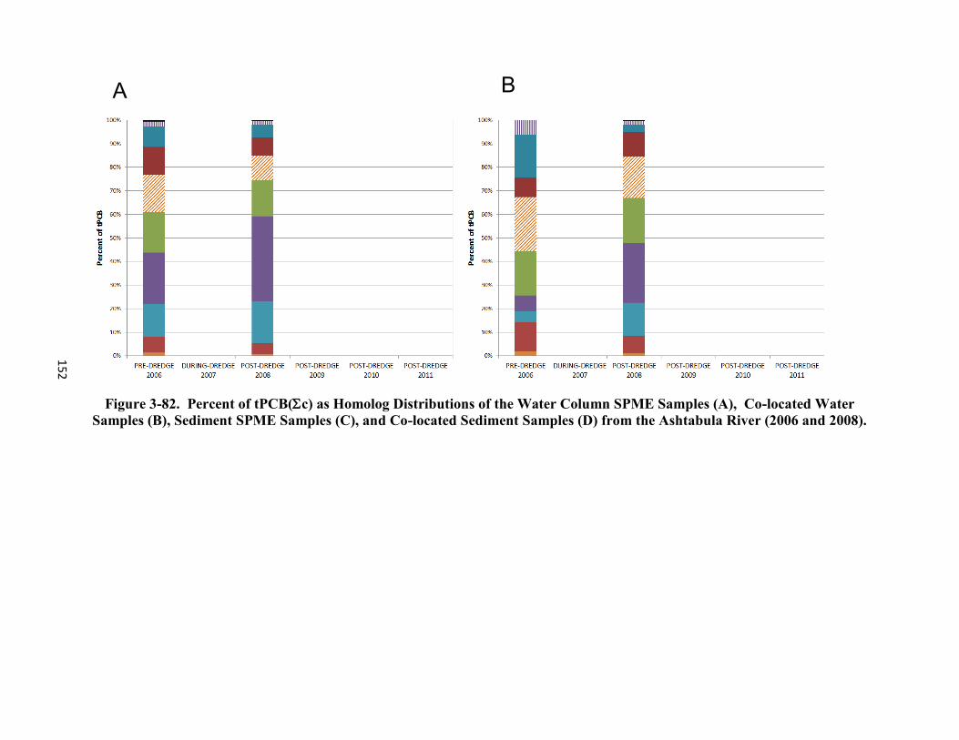
152

Figure 3-82. Percent of tPCB(c) as Homolog Distributions of the Water Column SPME Samples (A), Co-located Water Samples (B), Sediment SPME Samples (C), and Co-located Sediment Samples (D) from the Ashtabula River (2006 and 2008).

A B

153

Figure 3-82 (continued). Percent of tPCB(c) as Homolog Distributions of the Water Column SPME Samples (A), Co-located Water Samples (B), Sediment SPME Samples (C), and Co-located Sediment Samples (D) from the Ashtabula River (2006 and

2008).

C D

154

*Note: tPCB(c) Concentrations at Station 1 in 2006 and 2008 were below the detection limit, and ½ the detection

limit was reported.

Figure 3-83. tPCB(c) Concentration per SPME Placed on Surface Sediments from the Ashtabula River (2006 and 2008).

Figure 3-84. tPCB(c) Concentrations in Surface Sediment Samples Co-located with SPMEs from the Ashtabula River (2006 and 2008).

0

5

10

15

20

25

STATION1

STATION15

STATION3

STATION12

STATION11

STATION4

STATION10

STATION8

STATION7

STATION6

STATION5

tPC

B(

c)(n

g/S

PM

E)


PRE-DREDGE 2006

POST-DREDGE 2008

*

0

0.1

0.2

0.3

0.4

0.5

0.6

STATION 1

STATION 15

STATION 3

STATION 12

STATION 11

STATION 4

STATION 10

STATION 8

STATION 7

STATION 6

STATION 5

tPC

B(

c)(m

g/k

g d

ry)


PRE-DREDGE 2006

POST-DREDGE 2008

155

4.0 DISCUSSION An overall objective of this report was to evaluate selected methods to characterize pre-, during, and post-dredging physical, chemical and biological conditions within the ORD study area at the Ashtabula River. The primary means to achieve this objective was to assess each method’s ability to detect spatial or temporal change or both. Three general questions were defined to focus the assessment methods:

How effective is the method for detection of significant changes at individual locations and between reference locations and contaminated areas?

How effective is the method for detecting changes in chemical distributions or patterns in matrices?

How do the methods compare to one another? In this study, however, a direct comparison between methods was difficult because deployments were not always co-located. A qualitative discussion of overall findings among methods is included.

The methods assessed included the use of passive samplers (SPMDs and SPMEs) developed to complement or replace biota for chemical fate and transport studies associated with contaminants in aquatic systems. The biota tested included macrobenthic organisms, caged organisms such as fish and bivalves, and chemical concentrations in indigenous fish. A substantial amount of the data generated and discussed in this report relate to the macrobenthos samplers and the SPMD water and sediment samplers as well as their co-located sediment and water samples. Comparison of PCB concentrations measured by the appropriate method (i.e., the macrobenthos tissues and SPMDs) with the concentrations of their co-located sediment and water samples (when available) was performed using linear correlation. Statistical analyses were also used to assess whether change could be detected over time and space within and among co-located matrices and to compare the changes in PCB congener patterns over space and time. Limited data from the indigenous catfish study were also assessed. Data Screening Prior to statistical analyses, data generated for macrobenthos and fish tissues and sediment and water samples were screened by plotting the naïve observed data, and the averaged results were used in subsequent analysis. These plots are provided in Appendix I. 4.1 Macrobenthos Tissue Concentrations using Artificial Substrate Samplers The results from the macrobenthos sampling were evaluated with direct measures of PCB and PAH concentrations in co-located sediment and water samples using a linear correlation and an ANOVA model (Section 2.10). Table 4.1 summarizes the measurements by area, year, and sample type that are presented separately in Section 2 and it also expands on the tables by showing the actual sample numbers collected and available for statistical analysis. The locations of the macrobenthos stations are shown in Figure 2-10.

156

In addition, changes in chemical characteristics of the PCBs (i.e., congener patterns) were evaluated using PCA to evaluate the methods ability to distinguish changes pre- and post-dredging and to aid in assessing the usefulness of the methods in measuring the efficacy of environmental dredging. The specific questions that guided this assessment were:

Do the macrobenthos chemical data correlate with chemical composition in co-located sediments and water?

Do the macrobenthos chemical data correlate with changes in accumulated chemical patterns in tissue and co-located sediment and water data?

Do the macrobenthos chemical data correlate with passive sampler sampling methods (i.e., SPMDs and SPMEs)?

Table 4.1: Summary of Macrobenthos Study Samples used in ANOVA.

Year Area Macrobenthos(a) Macrobenthos

Water Samples(b)

Macrobenthos Sediment Samples(c)

2006

Upstream 2 1 0 Fields Brook 2 1 0 Turning Basin 2 1 0 River Bend 2 1 0 Reference 0 0 0

2007

Upstream 2 2 2 Fields Brook 2 2 2

Turning Basin 2 2 2 River Bend 2 2 2 Reference 0 0 0

2008


2009


2010

Upstream 2 3 2 Fields Brook 2 2 2 Turning Basin 2 2 2 River Bend 2 1 2

Table 4.1 (continued): Summary of Macrobenthos Study Samples used in ANOVA.

157

Year Area Macrobenthos(a) Macrobenthos

Water Samples(b)

Macrobenthos Sediment Samples(c)

Reference 2 2 2

2011

Upstream 4 0 1

Fields Brook 2 0 1

Turning Basin 2 0 1

River Bend 2 0 1

Reference 2 0 1

Values indicate the number of replicates included in the calculations of the average values used in the statistical analysis.

Macrobenthos data were not collected at Fields Brook in 2009 and were collected in four samples upstream in 2011.

Water samples were not collected in 2006 for tPAH16 and tPAH34 or at all in 2011.

Sediment samples (aside from PCB congeners) were not collected in 2006.

4.1.1 Macrobenthos ANOVA

To address the first question (change in time compared to reference), three ANOVA screening models, one model for the macrobenthos, one model for the SPMDs, and one model for their co-located sediments and waters, were developed (as described in Section 2.10). Graphic representations of the observed data aggregated by year and area with averages are included in Appendix C. The ANOVA compared the contamination levels by year and area sampled as follows:

Lipid-normalized tPCB(c), tPAH16, and tPAH34 in macrobenthos samples

Contaminants in sediment associated with macrobenthos samples

Contaminants in water associated with macrobenthos samples.

Overall, ANOVA model results for lipid-normalized macrobenthos samples are shown in Table 4.2 by chemical (tPCB(c), tPAH16, and tPAH34). The estimated MSE or variance, model r-square, and the p-values for the area and year fixed effects are shown. In all cases, the macrobenthos data were determined to be log-10 distributed and so the response for these models is the log-10 transformed average. Both year and area were significant for all models. A high tPAH value was noted in the Upstream macrobenthos data for 2009. Sensitivity analyses indicate that without this outlier, both factors remain significant, with r-square values 8% to 10% higher.

The effect of normalization was assessed by comparing the root MSEs in the above models with those using the un-normalized results. In general, this assessment resulted in minimal change in conclusions reached, as seen in Table 4.2.

158

Table 4.2: ANOVA Model Results for Raw and Lipid-Normalized Macrobenthos Factors.

Factor

Root Mean Square Error r-Square

p-Values

Year Area

Raw (Wet Wt) Macrobenthos Factors

tPCB(c) (mg/kg) 0.281 0.750 0.100 0.024*

tPAH16 (mg/kg) 0.240 0.672 0.246 0.033*

tPAH34 (mg/kg) 0.240 0.788 0.025* 0.028*

Lipid-Normalized Macrobenthos Factors

tPCB(c) (mg/kg) 0.236 0.865 0.015* 0.003*

tPAH16 (mg/kg) 0.160 0.867 0.006* 0.005*

tPAH34 (mg/kg) 0.172 0.906 0.001* 0.010*

* Statistically significant at the 0.05 level.

The least square means for year and area are represented in Tables 4.3 and 4.4, respectively. Note that p-values for yearly least square means are calculated after accounting for variance due to area and have been Bonferroni adjusted for five multiple comparisons in Table 4.3 and for three multiple comparisons in Table 4.4.

Table 4.3: Least Square Means and Confidence Intervals for Lipid-Normalized Macrobenthos Factor Results with Significant Pairwise Comparisons by Year.

Factor Year Least Square

Mean

95% Confidence

Interval Pairwise Significant

Differences

tPCB(c) (mg/kg lipid)

2006 118.4 (58.2, 240.9) 2008 < 2006 (p=0.038)

2007 115.1 (56.6, 234.3) 2009 < 2006 (p=0.038)

2008 26.1 (12.8, 53.1) 2011 < 2006 (p=0.038)

2009 23.5 (9.6, 57.4)

2010 40.3 (19.8, 82)

2011 26.7 (13.1, 54.4)

tPAH16 (mg/kg lipid)

2006 102.2 (63.2, 165.4) 2008 < 2006 (p=0.004)

2007 60.8 (37.6, 98.3) 2009 < 2006 (p=0.011)

2008 23.1 (14.3, 37.4) 2010 < 2006 (p=0.038)

2009 27.0 (14.7, 49.3) 2011 < 2006 (p=0.007)

2010 43.5 (26.9, 70.4)

2011 27.6 (17.1, 44.7)

Table 4.3 (continued): Least Square Means and Confidence Intervals for Lipid-Normalized Macrobenthos Factor Results with Significant Pairwise Comparisons by Year.

159

Factor Year Least Square

Mean

95% Confidence


Differences


2006 323.7 (192.6, 543.9) 2007 < 2006 (p=0.009)

2007 109.7 (65.3, 184.4) 2008 < 2006 (p<0.001)

2008 36.1 (21.5, 60.6) 2009 < 2006 (p=0.001)

2009 41.4 (21.6, 79.5) 2010 < 2006 (p=0.002)

2010 66.6 (39.6, 111.9) 2011 < 2006 (p<0.001)

2011 36.0 (21.5, 60.6)

The least square means estimates (i.e., variability of the data) and associated confidence intervals for lipid-normalized tPCB(Σc), tPAH16, and tPAH34 data by year (Figure 4-1) demonstrate graphically that concentrations of tPCB(Σc)s, tPAH16s, and tPAH34s decreased from 2006 to 2011. Moreover, the data set has less variability in the later years. The years that are statistically different from each other are summarized in Table 4.3.

Likewise, p-values for area least square means calculated after accounting for the variance due to year and a Bonferroni adjustment for a three multiple comparison indicate that Fields Brook had higher concentrations of tPCB(Σc)s in the macrobenthos comparisons and the data were more variable across the years.

Table 4.5 summarizes the mean measurement values for each of the response variables for the Upstream and Conneaut Creek Reference locations by year; these values were not included in the ANOVA models. Table 4.6 lists the overall mean measurements for the Upstream and Conneaut Creek Reference locations for each of the response variables.

Table 4.4: Least Square Means and Confidence Intervals for Lipid-Normalized Macrobenthos Factor Results with Significant Pairwise Comparisons by Area.

Factor Area Least

Square Mean

95% Confidence


Differences

tPCB(c) (mg/kg lipid)

Turning Basin 45.1 (27.2, 74.7) Turning Basin < Fields Brook (p=0.034)

River Bend < Fields Brook (p=0.002)

Fields Brook 122.5 (69.9, 214.7)

River Bend 22.6 (13.7, 37.5)


Turning Basin 52.7 (37.5, 74.2) River Bend < Turning Basin (p=0.016)

River Bend < Fields Brook (p=0.008)

Fields Brook 61.2 (41.8, 89.4)

River Bend 24.3 (17.2, 34.1)

Table 4.4 (continued): Least Square Means and Confidence Intervals for Lipid-Normalized Macrobenthos Factor Results with Significant Pairwise Comparisons by Area.

160

Factor Area Least

Square Mean

95% Confidence


Differences


Turning Basin 96.3 (66.7, 139.2) River Bend < Turning Basin (p=0.021)

Fields Brook 98.7 (65.5, 148.7)

River Bend 43.4 (30, 62.7)

The least square mean value for the Fields Brook location was significantly greater than the least square mean values for both the Turning Basin and River Bend locations for tPCB(Σc). The least square mean value for the River Bend location was significantly less than the least square mean values for both the Turning Basin and Fields Brook locations for tPAH16. For tPAH34, the least square mean value was significantly less at the River Bend location when compared to the least square mean for the Turning Basin location.

The least square means for each year for the combined Turning Basin, Fields Brook, and River Bend areas for tPCB(Σc), tPAH16, and tPAH34, respectively, are shown in Figure 4-1. The least square geometric means along with corresponding confidence intervals for each of the three locations (all years) are displayed in Figure 4-2. Note that since a log transform was necessary for the model, geometric means and confidence intervals are provided, which result in confidence bounds that are not symmetric about the geometric mean.

161

* This year was significantly different from 2006 at the 0.05 significance level.



Figure 4-1. Least Square Means for Lipid-Normalized Macrobenthos tPCB(Σc) (A); tPAH16 (B); and tPAH34 (C) (mg/kg Lipid) Measurements in Fields Brook, Turning

Basin, and River Bend Stations by Year with 95% Confidence Intervals.

0

50

100

150

200

250

2006 2007 2008* 2009* 2010 2011*

tPC

B(Σ

c) (m

g/kg

lipid

)

Year

0

50

100

150

200

2006 2007 2008* 2009* 2010* 2011*

tPA

H1

6 (

mg/

kglip

id)

Year

0

100

200

300

400

500

600

2006 2007* 2008* 2009* 2010* 2011*

tPA

H3

4 (

mg/

kg li

pid)

Year

A

B

C

162

Table 4.5: Means for Lipid-Normalized Macrobenthos Chemical Measurements by Year for Upstream and Conneaut Creek Reference.

Measurement Location 2006 2007 2008 2009 2010 2011 tPCB(Σc) (mg/kg lipid) Upstream 21.702 12.400 7.013 11.213 0.140 0.659

tPCB(Σc) (mg/kg lipid)

Conneaut Creek Reference NA NA NA 1.082 0.126 1.470

tPAH16 (mg/kg lipid) Upstream 251.128 230.472 63.181 514.668 53.341 9.877



tPAH34 (mg/kg lipid) Upstream 552.225 338.975 86.822 680.239 69.419 11.156



NA - No data were available for this year * This year was significantly different from 2006 at the 0.05 significance level

Table 4.6: Means for Lipid-Normalized Macrobenthos by Measurement for Upstream and Conneaut Creek References.

Measurement Upstream Conneaut Creek Reference

tPCB(Σc) 8.855 0.893 tPAH16 187.111 10.930 tPAH34 289.806 15.513

4.1.2 Macrobenthos PCA

PCA was used to explore differences in congener compositions measured in macrobenthos tissues across locations and years. The PCA analysis tested whether the PCBs in the study region could be related to Aroclor compositions and whether the pre- and post-dredge samples reflected substantial change after the remedial dredging. The analysis suggests the PCBs taken up by the macrobenthos deployed at the Upstream and Conneaut Creek Reference cluster together in the upper left side of the PCA graph for all years and tend to overlap with the Aroclor 1268 signature (Figure 4-3). In contrast, the 2007 through 2011 Turning Basin and River Bend macrobenthos data cluster in the upper right side of the PCA graph near Aroclors 1248 and 1254. All Fields Brook samples cluster tightly within the larger Aroclor 1248 and 1254 signature. The 2006 Turning Basin and River Bend samples are outliers and fall within the same general area as Aroclors 1260 and 1262. The cumulative variance was 47%.

163

Figure 4-2. Least Square Means for Lipid-Normalized Macrobenthos tPCB(Σc) (A), tPAH16 (B), and tPAH34 (C) (mg/kg lipid) Measurements in Turning Basin, Fields Brook,

and River Bend Stations by Area with 95% Confidence Intervals.

0

50

100

150

200

250

Turning Basin Fields Brook River Bend

tPC

B(Σ

c) (

mg/

kg li

pid

)

Location

0

50

100

150

200


tPA

H1

6 (

mg/

kg li

pid

)

Location

0

100

200

300

400

500

600


tPA

H3

4 (

mg/

kg li

pid

)

Location

A

B

C

164

Area Symbol Color




River Bend RBxx Red

Conneaut Creek Reference RFxx Green

“xx” represents year

Figure 4-3. PCA for Macrobenthos tPCB(c) (All Stations, All Years).

4.1.3 ANOVA Analysis of Surface Sediment for Macrobenthos Stations

The raw (dry wt), TOC-normalized, and percent fines-normalized sediment tPCB(c), tPAH16, and tPAH34 ANOVA screening model results are shown in Table 4.7. This table summarizes estimated MSE, model r-square, and p-values for the year and area fixed effects. Area was significant for tPCB(Σc) congeners normalized to TOC. The effect of normalization was assessed by comparing the root MSEs in the models to one another. Normalizing to TOC produced a large benefit for both tPAH16 and tPAH34 (MSE difference = 5216.7 and 9385.4,

-6 -4 -2 0 2 4 6

-15

-10

-50

Macroinvertebrate

Cumulative Variance Explained: PC1 29 %; PC2 47 %PC1

PC2

FB08FB08RB08

RB08

TB08

TB08

UP08

UP08 FB06FB06

RB06

RB06

TB06

TB06

UP06

UP06

FB07FB07RB07 RB07TB07

TB07

UP07 UP07

RF09 RF09

RB09RB09TB09TB09

UP09

UP09FB10FB10

RF10RF10

RB10RB10TB10

TB10

UP10UP10RF11RF11

FB11FB11

RB11RB11

TB11

TB11UP11UP11

UP11UP11

A1221

A1232A1016A1242A1248

A1254

A1260A1262

A1268

Aroclor 1268

Aroclor 1254

Aroclors 1232, 1016, and 1242

Aroclors 1260 and 1262

165

respectively) and a somewhat smaller benefit for tPCB(Σc) (MSE difference = 0.152). Normalizing to percent fines demonstrated an additional benefit for tPAH16 and tPAH34 (MSE difference = 186.6 and 347, respectively), but no benefit for tPCB(Σc) (MSE difference = -0.331). The effect of area was only significant for tPCB(Σc); the corresponding results are presented in Table 4.8.

Table 4.7: Screening ANOVA Model Results for Sediment Samples Associated with Macrobenthos Sample Factors.

Factor Root Mean Square Error r-Square p-Values

Year Area

Raw(Dry Weight) Macrobenthos Factors

tPCB(Σc) (mg/kg Dry) (a) 0.560 0.522 0.697 0.055

tPAH16 (mg/kg Dry) 5.410 0.415 0.547 0.351

tPAH34 (mg/kg Dry) 9.745 0.390 0.700 0.291

TOC-Normalized Factors

tPCB(Σc) (mg/kg Dry) (a) 0.408 0.655 0.528 0.027*

tPAH16 (mg/kg Dry) 0.194 0.403 0.745 0.239

tPAH34 (mg/kg Dry) 0.360 0.395 0.869 0.197

Percent Fines-Normalized Factors

tPCB(Σc) (mg/kg Dry) (a) 0.739 0.468 0.780 0.131

tPAH16 (mg/kg Dry) 0.007 0.392 0.382 0.832

tPAH34 (mg/kg Dry) 0.013 0.320 0.609 0.643

(a) tPCB(Σc) congeners normalized to both TOC and percent fines were found to be log-base10 distributed. * Statistically significant at the 0.05 level.

Further examination of the least squares means for area for tPCB(Σc) congeners normalized to TOC are presented in Table 4.8. Note that p-values for area least square means are calculated after accounting for variance due to year and after they have been Bonferroni adjusted for three multiple comparisons. Figure 4-4 presents the least square mean estimates and associated confidence intervals for these factors by area.

166

Table 4.8: Least Square tPCB(Σc) Means and Confidence Intervals for Sediment Sample Measurements Associated with Macrobenthos Samples with Significant Pairwise

Comparisons by Year.

Factor Area Least Square Mean

95% Confidence Interval

Pairwise Significant Differences

tPCB(Σc)

(mg/kg OC)

Turning Basin 0.011 (0.004, 0.028) River Run < Turning Basin (p=.033) Fields Brook 0.007 (0.003, 0.018)

River Bend 0.002 (0.001, 0.004)

Figure 4-4. Least Square Means for tPCB(Σc) Normalized to TOC (mg/kg Dry) Sediment Sample Measurements Associated with Macrobenthos Samples by Area with 95%

Confidence Intervals. 4.1.4 Surface Sediment PCA

PCA was used to explore differences in congener compositions measured in surface sediment co-located with the macrobenthos stations across locations and years. The PCA graph for macrobenthos surface sediment is similar to the macrobenthos PCA graph with the Upstream and Conneaut Creek Reference samples clustering in the upper left side of the PCA graph in the general vicinity of Aroclor 1268 (Figure 4-5). The Turning Basin, River Bend, and Fields Brook samples all cluster together in the upper right side of the PCA graph near Aroclor 1248. The 2006 Turning Basin and 2006 River Bend sediment samples again are the outliers, similar to the macrobenthos samples. The 2007 River Bend and 2010 Fields Brook samples also do not appear where expected based on the other data and cluster around Aroclor 1254. The cumulative variance was 57%.

0

0.005

0.01

0.015

0.02

0.025

0.03


tPC

B(Σ

c) (

mg/

kg O

C)

Location

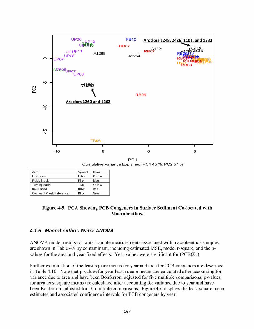
167

Area Symbol Color




River Bend RBxx Red


Figure 4-5. PCA Showing PCB Congeners in Surface Sediment Co-located with Macrobenthos.

4.1.5 Macrobenthos Water ANOVA

ANOVA model results for water sample measurements associated with macrobenthos samples are shown in Table 4.9 by contaminant, including estimated MSE, model r-square, and the p-values for the area and year fixed effects. Year values were significant for tPCB(c). Further examination of the least square means for year and area for PCB congeners are described in Table 4.10. Note that p-values for year least square means are calculated after accounting for variance due to area and have been Bonferroni adjusted for five multiple comparisons; p-values for area least square means are calculated after accounting for variance due to year and have been Bonferroni adjusted for 10 multiple comparisons. Figure 4-6 displays the least square mean estimates and associated confidence intervals for PCB congeners by year.

-10 -5 0 5

-15

-10

-50

Sediment


PC2

FB08RB08

TB08

UP08

FB08

RB08

TB08UP08 FB06

RB06

TB06

UP06

FB07

RB07

TB07UP07

FB07

RB07

TB07

UP07

FB09FB09

RF09

RF09

RB09RB09TB09

TB09TB09TB09

UP09

UP09

FB10

FB10

RF10RF10

RB10RB10TB10

TB10

UP10

UP10RF11

FB11

RB11TB11

UP11A1221

A1232A1016A1242A1248

A1254

A1260A1262

A1268

Aroclors 1260 and 1262

Aroclors 1248, 2426, 1101, and 1232

168

Table 4.9: ANOVA Model Results for Water Sample Measurements Associated with Macrobenthos Sample Factors.

Factor MSE r-Square

p-Values

Year Area

tPCB(Σc) (ng/L Liquid) 39.362 0.760 0.026* 0.162

tPAH16 (ng/L Liquid) 55.805 0.703 0.078 0.216

tPAH34 (ng/L Liquid) 78.160 0.713 0.063 0.294

* Significant at the 0.05 level of significance.

Table 4.10: Least Squares Means and Confidence Intervals for Water Sample Measurements Associated with Macrobenthos Samples Factors.

Factor Year Least Squares

Mean 95% Confidence


Differences

tPCB(c) (ng/L Liquid)

2006 132.404 (80.288, 184.52) 2009 < 2006 (p=0.028)

2007 114.906 (62.789, 167.022) 2010 < 2006 (p=0.031)

2008 55.595 (3.478, 107.711)

2009 24.827 (-20.723, 70.377)

2010 32.380 (-13.17, 77.93)


Figure 4-6. Least Squares Means for tPCB(Σc) (ng/L Liquid) Sample Measurements Associated with Macrobenthos Samples by Year with 95% Confidence Intervals.

-50.00

0.00

50.00

100.00

150.00

200.00

2006 2007 2008 2009* 2010*

tPC

B(Σ

c) (m

g/L

Liq

uid)

Year

169

Table 4.11 lists the mean tPCB(Σc) (ng/L liquid) measurements by year for the Upstream and Conneaut Creek Reference locations, which were not included in the ANOVA model.

Table 4.11: Means for tPCB(Σc) (ng/L Liquid) Sample Measurements by Year for Upstream and Conneaut Creek Reference

Location 2006 2007 2008 2009 2010 2011 Upstream 49.450 17.088 15.885 17.455 11.570 49.450 Conneaut Creek Reference NA NA NA 17.578 15.638 NA

NA: No data were available for this year.

4.1.6 PCA for Waters from Macrobenthos Stations

PCA was used to explore differences in congener compositions measured in water samples co-located with the macrobenthos tissue samplers across locations and years. The PCA graph for macrobenthos water samples is very different from the macrobenthos PCA graph and the surface sediment PCA graph (Figure 4-7). In the water PCA analysis, the 2007 Fields Brook, River Bend, and Turning Basin samples all clustered in the upper left corner of the PCA graph. The 2008, 2009, and 2010 data are in close proximity to one another, but not in the same tight cluster as before and closer to Aroclor 1254 and Aroclor 1268. The cumulative variance was 48%.

4.1.7 Comparison of Macrobenthos Tissue and Co-located Sediment and Water

PCBs

4.1.7.1 Correlation Analysis

A simple linear correlation was performed using tPCB(c) data (normalized to lipids) from all stations and all years and tPCB(c) in co-located sediment (normalized to TOC) and co-located surface water (Figure 4-8). Little correlation was observed between the tissue and sediment data. A somewhat stronger correlation was observed between tPCB(c) in macrobenthos tissue and co-located tPCB(c) in the surface water. Uptake of PCBs by the macrobenthos occurs primarily through contact with the water column, so this observation is not unexpected.

170

Area Symbol Color




River Bend RBxx Red


Figure 4-7. PCA Showing PCB Congeners in Waters with Macrobenthos Samples. 4.1.7.2 PCA Comparing Macrobenthos Tissues, Sediment, and Water

PCA showing PCB congener distribution of macrobenthos tissues, and co-located sediments and waters is presented in Figure 4-9. Interestingly, the sediment along with tissue patterns for all locations except the upstream sites in all years and the River Bend and Turning Basin in 2006 cluster near to each other, between A1248 and A1254. This would seem to indicate that the PCB patterns observed in the tissues during this time frame reflect what is observed in the sediments. The upstream sites for sediment and tissue appear to cluster around the heavier Aroclor 1260/1268, indicating that the composition of PCBs in this location is different from the downriver sites. This should be interpreted that the PCB congeners are of a similar make-up regardless of whether they are derived from water, sediment, or tissue samples.

-10 -5 0 5

-15

-10

-50

Water


PC2

FB08

RB08

TB08UP08

FB08

RB08

TB08

UP08

FB07RB07TB07

UP07

FB07

RB07TB07

UP07FB10RF10

TB10

UP10FB09

FB09

RF09

RF09

RB09RB09

TB09TB09TB09

TB09

UP09UP09FB10 RF10RB10TB10

UP10UP10A1221

A1232A1016A1242A1248

A1254

A1260A1262

A1268

Aroclors 1248, 1242, 1232, and 1016

Aroclor 1268

171

Figure 4-8. Correlation Plot between tPCBs(c) in Macrobenthos Tissues and Co-located Sediments (TOC Normalized) and Waters.

172

Code: XX##, where XX = station and ## = year

Figure 4-9. PCA Showing PCB Congeners in Macrobenthos Tissue and Co-located Surface Sediments and Waters.

4.2 SPMDs SPMDs were used to measure integrated in situ PCB concentrations from either the water column or porewater. Water concentrations were calculated from the water column SPMDs to compare with the PCBs directly measured in the water column both with and without the PRC recoveries. Sediment SPMD results were used to calculate porewater concentrations; however, direct porewater measurements were not determined during this study. Comparisons were made between the concentrations found in both types of SPMDs to the co-located water and sediment measurements using a linear correlation model. ANOVA was performed to determine significance differences over time and space of the PCBs in the water column SPMD and co-located water samples only.

-6 -4 -2 0 2 4 6

05

1015

Combined


PC2

FB08FB08RB08

RB08

TB08

TB08

UP08

UP08

FB06FB06

RB06

RB06

TB06

TB06

UP06 UP06

FB07FB07RB07RB07

TB07TB07UP07

UP07

RF09RF09

RB09RB09TB09TB09

UP09UP09

FB10FB10

RF10RF10

RB10RB10TB10

TB10

UP10UP10RF11RF11

FB11FB11

RB11RB11

TB11TB11

UP11UP11UP11UP11

FB08RB08TB08

UP08

FB08RB08

TB08

UP08

FB06

RB06

TB06

UP06

FB07RB07

TB07

UP07

FB07RB07

TB07

UP07

FB09FB09

RF09

RF09

RB09RB09TB09

TB09TB09TB09

UP09

UP09

FB10

FB10

RF10RF10

RB10RB10TB10TB10

UP10

UP10

RF11

FB11RB11

TB11

UP11

FB08 RB08TB08

UP08

FB08

RB08

TB08

UP08

FB07RB07TB07 UP07

FB07RB07TB07

UP07

FB10RF10TB10 UP10

FB09

FB09 RF09

RF09

RB09RB09TB09TB09TB09

TB09

UP09UP09FB10

RF10

RB10

TB10 UP10UP10A1221

A1232A1016A1242

A1248

A1254

A1260A1262

A1268

MacroinvertebrateSedimentWaterAroclor

Aroclor 1254

Aroclor 1260 & 1262

Aroclor 1248

173

4.2.1 Correlation between SPMDs and Co-Located Sediments and Waters

PCBs measured in the water column were made on whole water samples, not filtered samples, and SPMDs would not accumulate particle-associated chemicals. As such, no correlation was observed between the concentrations found in the water column SPMDs compared to the actual measured water concentrations either on a ng/SPMD or ng/L basis. It is interesting to note, however, that the water column concentrations in 2006 were much higher than those measured in subsequent years (post-dredging); however, this difference was not observed in the water column SPMDs (Figures 4-10 and 4-11). However, as noted in Section 3.5.1.1, these higher water column concentrations are likely a result of high particulates in the water column.

Figure 4-10. Correlation between Water Column SPMD and Co-located Whole Water Sample tPCB(C) Concentrations.

174

Figure 4-11. Correlation between Water Column SPMD Estimated Water and Co-located Whole Water Sample tPCB(C) Concentrations.

Additional evaluation of the data sets (2006 and 2008/2011) across sampling stations within a single year did not reveal any localized correlation between water column measurements and SPMD measurements (Figures 4-12 and 4-13).

Note: Chart symbols are labelled with the Station ID.

Figure 4-12. Correlation between 2006 Water Column SPMD (ng/SPMD) and Co-located Whole Water Sample tPCB(C) Concentrations by Stations.

175

Note: Chart symbols are labelled with the Station ID.

Figure 4-13. Correlation between 2008/2011 Water Column SPMD (ng/SPMD) and Co-located Whole Water Sample tPCB(C) Concentrations by Station.

Evaluation of sediment SPMD data sets compared to the co-located sediment results exhibited similar, but little, correlation (R2 = 0.0071) (Figure 4-14). This was also the case when the apparent outlier from 2011 (Water tPCB[C]) = 3331 ng/L) was removed from the correlation (R2 = 0.0095). Comparison of sediment SPMD estimated PCB concentrations vs. co-located overlying water column results revealed a somewhat better correlation (Figure 4-15).

Figure 4-14. Correlation between Sediment SPMD (ng/SPMD) and Co-located Sediment Sample tPCB(C) Concentrations.

R² = 0.0071

0

500

1000

1500

2000

2500

0 500 1000 1500 2000 2500 3000 3500

SED

SP

MD

tP

CB

(C

) (n

g/SP

MD

)

Co-located Sediment tPCB(C) (ng/g dry)

2006

2008

2011

176

Figure 4-15. Correlation between Sediment SPMD (ng/L) and Co-located Whole Water Sample tPCB(C) Concentrations.

4.2.2 Water Column SPMD ANOVA

A two-way ANOVA was performed to evaluate the effects of year and station on PCBs in the water column SPMDs. The average level is modeled to be a constant average plus an offset for additive effects for year and station, where the constant (intercept) is the estimated level for Station 3 of year 2006. For SPMD concentrations, some 2006 observations were notably higher than the rest of the data, making the range in the values wider in 2006 than the following years. However, the PCB levels are generally of the same order of magnitude, and the residuals from each of the ANOVA models are approximately normally distributed with a zero mean. Therefore, the ANOVA was performed on the natural scale. Visual inspection of quantile-quantile plots (not shown) indicated that the residuals were approximately normally distributed for each response; in all cases, the Shapiro statistic for non-normality was not significant. The year effect was significant for all responses except the equivalent water concentrations using PRC when the analysis includes Station 25 2006 values. If Station 25 2006 is excluded from the latter analysis, the effect of year is significant. The effect of station is only significant for the co-located water concentrations. Table 4.12 summarizes the model results. ANOVA indicates that the effect of year is significant (p= 0.013) and the effect of station is not statistically significant (p=0.299). Neither year nor station has significant effect on water concentrations estimated from the PRC when all the data are included. Year effect is significant for the co-located water concentrations (p<0.0001). For this response, the effect of station is also significant (p=0.0003). The 2006 observation for Station 25 has a very large residual that contributes to a high estimate of mean square error. If the analysis is repeated with this observation excluded, the effect of

R² = 0.2959

0

2

4

6

8

10

12

14

16

18

0 20 40 60 80 100 120

SED

SP

MD

Est

imat

ed

Wat

er

PC

B

Co

nce

ntr

atio

ns

(ng/

L) U

sin

g P

RC

s

Co-located Water tPCB(C) (ng/L)

2006

2008 & 2011

177

year is significant (p=0.033). All subsequent evaluations of these data excluded Station 25 results from 2006.

Table 4.12: Results of the Two Way ANOVA for Water Column SPMDs and Co-located

Water Samples.

Factor Root Mean Square Error r-Square

p-Values

Year Station

tPCB(Σc)s (ng/SPMD) 617.0 0.576 0.013* 0.299

Estimated Water Concentration (ng/L) using PRCs (Including Station 25 2006) 1.5 0.517 0.101 0.249

Estimated Water Concentration (ng/L) using PRCs (Excluding Station 25 2006) 1.1 0.621 0.033* 0.113

Estimated Water Concentration (ng/L) NOT using PRCs 4.3 0.576 0.013* 0.299

Co-located Water Concentration (ng/L) (Excluding Station 25 2006) 4.2 0.992 <0.0001* <0.0001*


SPMD tPCB(Σc) (ng/SPMD). The post-hoc pairwise analysis of SPMD (ng/g SPMD) results by year (pooling all station locations) indicates that the decrease in average PCB levels across stations from 2006 to 2011 is statistically significant (Table 4.13). However, no significant change was observed between other years.

Table 4.13: Least Squares Means and Confidence Intervals for SPMD tPCB(Σc) (ng/SPMD).

Factor Year Least Squares Mean 95% Confidence Interval


tPCB(Σc) (ng/SPMD)

2006 2140.64 (1691.4, 2589.8) 2011<2006 (p=0.0141) 2008 1844.60 (1373.5, 2315.7)

2011 1329.36 (880.2, 1778.6)

Estimated Water Concentrations using PRCs. The post-hoc pairwise analysis of estimated water concentration (ng/L) results by year (pooling all station locations) indicate that the change in average PCB levels across stations from 2008 to 2011 is statistically significant (Table 4.14). Unlike the other responses, the change in concentrations actually increased from 2008 to 2011. However, no significant change was observed between other years. The analysis indicates a significant year-to-year variability, but this variability is not indicative of a trend for this response.

Co-located Water Concentrations. The post-hoc pairwise analysis of co-located water concentration (ng/L) results by year (pooling all station locations) indicate that the decreases in average PCB levels across stations from 2006 to 2008 and from 2006 to 2011 are statistically significant (Table 4.15).

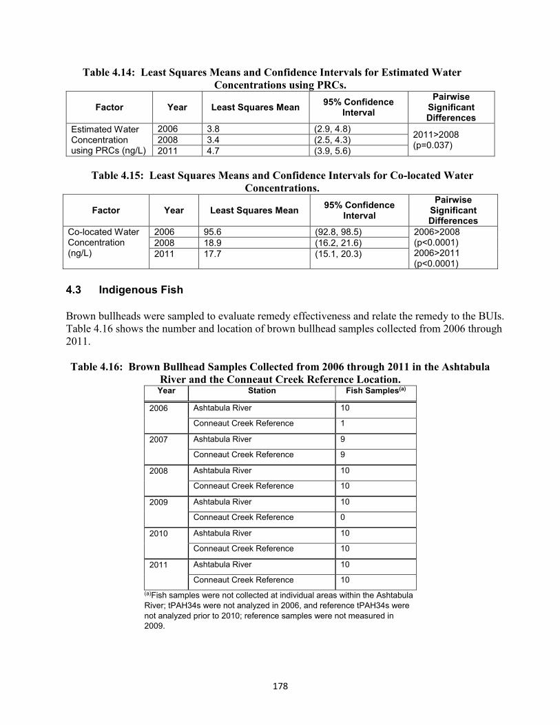
178

Table 4.14: Least Squares Means and Confidence Intervals for Estimated Water Concentrations using PRCs.



Estimated Water Concentration using PRCs (ng/L)

2006 3.8 (2.9, 4.8) 2011>2008 (p=0.037) 2008 3.4 (2.5, 4.3)

2011 4.7 (3.9, 5.6)

Table 4.15: Least Squares Means and Confidence Intervals for Co-located Water Concentrations.



Co-located Water Concentration (ng/L)

2006 95.6 (92.8, 98.5) 2006>2008 (p<0.0001) 2006>2011 (p<0.0001)

2008 18.9 (16.2, 21.6) 2011 17.7 (15.1, 20.3)

4.3 Indigenous Fish Brown bullheads were sampled to evaluate remedy effectiveness and relate the remedy to the BUIs. Table 4.16 shows the number and location of brown bullhead samples collected from 2006 through 2011. Table 4.16: Brown Bullhead Samples Collected from 2006 through 2011 in the Ashtabula

River and the Conneaut Creek Reference Location. Year Station Fish Samples(a)

2006

Ashtabula River 10

Conneaut Creek Reference 1

2007

Ashtabula River 9


2008

Ashtabula River 10


2009

Ashtabula River 10


2010

Ashtabula River 10


2011

Ashtabula River 10

Conneaut Creek Reference 10 (a)Fish samples were not collected at individual areas within the Ashtabula River; tPAH34s were not analyzed in 2006, and reference tPAH34s were not analyzed prior to 2010; reference samples were not measured in 2009.

179

4.3.1 ANOVA for Fish Tissue Chemistry

ANOVA was conducted on the fish data for tPCB(c), “Common” tPCB(Σc) (see Section 3.4.2.1 for discussion of tPCB(Σc) determination for fish samples), tPAH16, and tPAH34 (Table 4.17). There was not a significant difference among concentrations measured in fish at either the Reference location or within the Ashtabula River by area or over time (Table 4-17). The effect of lipid normalization of the contaminant tissue data was assessed by comparing the root mean square errors in the above models with those using the non-normalized results. In general, there is little change in conclusions as is seen in Table 4.17, but area was significant for the concentrations of tPCB(c) and the “Common” tPCB(c) in fish caught within the Ashtabula River. These concentrations were significantly different than those for fish collected at the Conneaut Creek Reference location. In addition, the root mean square errors were much smaller using non-normalized factors. Further examination of the least squares means of tPCB(c)s calculated using all available congeners as well as the “common” PCB list by area is provided in Table 4.18. This analysis shows that using the ‘common list’ of PCB congeners did not have an effect on the evaluation of the fish results. Note that p-values for year least squares means were calculated after accounting for variance due to year. Figures 4-16 and 4-17 display the least squares means estimates and associated confidence intervals for tPCB(c) by area using both calculation methods. In Table 4.18, the least square means for Conneaut Creek Reference for each Factor is set to 0 since the ANOVA model gives a negative value for each measurement. Additionally, the lower bound of the 95% confidence interval is also truncated at 0 since a negative concentration does not make sense in the context of the problem.

180

Table 4.17: ANOVA Model Results for Fish Factors.

Factor Root Mean

Square Error r-Square

p-Values

Year Area

Wet Weight Fish Factors

tPAH16 (mg/kg) 0.046 0.616 0.469 0.648

tPAH34 (mg/kg) 0.068 0.984 0.201 0.655

tPCB(Σc) (mg/kg) 1.077 0.805 0.461 0.056

Common tPCB(Σc) List (mg/kg) 0.888 0.793 0.475 0.063

Lipid-Normalized Fish Factors

tPAH16 (mg/kg lipid) 0.946 0.497 0.866 0.261

tPAH34 (mg/kg lipid) 1.383 0.970 0.301 0.403

tPCB(Σc) (mg/kg lipid) 22.806 0.860 0.373 0.031*

Common tPCB(Σc) List (mg/kg lipid) 18.940 0.847 0.395 0.036*


Table 4.18: Least Squares Means and Confidence Intervals for Fish Sample Measurements

with Significant Pairwise Comparisons by Area.

Factor Area Least Square

Mean 95% Confidence

Interval

tPCB(c) (mg/kg) Ashtabula River 60.935 (27.684, 94.185)

Conneaut Creek Reference 0.000* (0.000*, 36.062)

Common tPCB(c) List (mg/kg)

Ashtabula River 47.684 (20.071, 75.298)

Conneaut Creek Reference 0.000* (0.000*, 30.32)

* The value is set to zero since the model returns a negative value.

181

Figure 4-16. Least Squares Means for tPCB(c) Normalized to Lipids (mg/kg Lipid) Calculated using tPCB(c) Fish Sample Measurements by Area with 95% Confidence

Intervals.

Figure 4-17. Least Squares Means for tPCB(c) Normalized to Lipids (mg/kg Lipid) Calculated using Common Congener Fish Sample Measurements by Area with 95%

Confidence Intervals. 4.3.2 PCA for Fish

The fish collected from the Ashtabula River each year (2006 to 2011) were evaluated using PCA. Some of the years had much less variability within the samples compared to the other years (Figure 4-18). The 2006 Ashtabula River samples clustered together in the middle to lower left of the graph. The 2007 data clustered together in the bottom of the graph. The 2008, 2009, 2010, and 2011 samples are all clustered together in the upper left corner of the plot. The cumulative variance was 51%. Fish were collected throughout the river in each year and direct exposure in any given year may have been different; however, these results appear to show that fish from 2006 (pre-dredging) and 2007 (during dredging) appear to have accumulated different PCB compositions than fish collected from post-dredging conditions from 2008 through 2010.

0

20

40

60

80

100

Ashtabula River Conneaut Creek Reference

tPC

B(Σ

c) (m

g/kg

lipi

d)

0

10

20

30

40

50

60

70

80

Ashtabula River Conneaut Creek Reference

Co

mm

on

tP

CB

(Σc)

(mg/

kg

lipid

)

182

Note: Code = Fish #.Year Pink = 2006 Gray = 2007 Blue = 2008 Purple = 2009 Green = 2010 Yellow = 2011 Black = Aroclor

Figure 4-18. PCA using tPCB(c) for Brown Bullheads from the Ashtabula River from 2006 through 2011.

-5 0 5 10 15 20

-10-5

05

Fish

Cumulative Variance Explained: PC1 31.7 %; PC2 50.7 %PC1

PC2

03.06

08.0609.06 10.0611.06

12.0604.0605.06

06.06

07.06

01.07

02.07 03.07

04.07

05.07

06.0707.07 08.07

09.07

01.08

10.08

11.08

03.0804.08

05.08

06.08

07.08

08.08

09.08

01.09

10.0902.09

03.0904.09

05.09

06.09

07.09

08.09

09.09

01.10

10.10

02.1003.10

04.1005.10

06.1007.10

08.10 09.10

01.11

02.11

03.11

04.11

05.11

06.11

07.11

08.11

09.1110.11

A1221

A1232A1016

A1242

A1248A1254

A1260A1262

A1268

Aroclor 1254

Aroclors 1260

& 1262

183

5.0 CONCLUSIONS This research project was designed to develop and evaluate methods and metrics based on physical, chemical, and biological lines of evidence (LOEs) for characterizing sediment and ecosystem response to remediation, and more specifically to environmental dredging. A further objective was to develop methods and define an approach for measuring and characterizing sediment residuals formation during environmental dredging. The methods generated for evaluating dredge residuals were thoroughly discussed in “Field Study on Environmental Dredging Residuals: Ashtabula River, Volume 1. Final Report” (EPA, 2010). This report incorporates the 2010 findings with additional focus placed on the fate and transport of sediments and contaminants during dredging operations, biological response to remediation, and surface sediment chemistry as of the last comprehensive survey conducted in 2011. The conclusions below summarize observations noted during the data interpretation process and recommendations on the utility of the methods employed to obtain field measurements for evaluating remedy effectiveness. 5.1 Water Sampling during Dredging – Turbidity Measurements Environmental dredging, by design, seeks to minimize off-site migration of sediment suspended and chemicals of concern (COCs) during operations. With a goal of rapidly identifying mechanisms and minimizing their contributions to dredge residuals, field instrumentation can be used to monitor suspended sediment in dredge plumes permitting real-time or near real-time measurements during remediation activities. In contrast, collection of field samples followed by laboratory analyses results in a significant time lag from dredging implementation to measurement and documentation of residuals. This delay does not allow for field operations changes in a timely manner to minimize generation of residuals and off-site migration of COCs. Given the decreasing cost, greater availability of field monitoring instrumentation, and improved user interface and data processing, it is strongly recommended that real-time turbidity measurements be employed whenever possible to permit rapid feedback of dredge plume information to the on-site project management team during field operations. Advantages and disadvantages of using optical and acoustical backscatter methods exist for the measurement of TSS. Optical and acoustical backscatter signals are both proxies for particle concentration. Both techniques require careful calibration of backscatter against field samples of TSS, the success of which is highly dependent on field sampling protocols and spatial and temporal correlation of measurements. Optical and acoustic backscatter are also both sensitive to particle shape (theories for both assume spherical particles) as well as particle size. Optical techniques for estimating TSS can lead to overestimates of particle concentrations for smaller particle size distributions. Errors associated with optical derivations of TSS are small for well-sorted sediments. Errors are greatest when only a small amount of fine material is present because this material dominates the optical backscatter response. As such, errors in concentration estimates are smallest when the size distribution of the calibration sediment closely matches the size distribution of the measured suspended sediments.

184

Optical backscatter is also sensitive to density and composition of the particles and the ratio of optical backscattering to total scattering increases with the bulk index of refraction of particles; hence, denser particles will result in higher backscatter ratios regardless of concentration or size. Another limitation of optical turbidity sensors is that they provide measurements at only one location per sensor, although multi-sensor arrays are becoming increasingly feasible as technology and affordability improve. Importantly, optical sensors are also highly susceptible to biofouling, particularly in productive inland waters and, therefore, require a comprehensive operations and maintenance plan to provide high quality data. These reductions in data quality for optical sensors are not correctable, i.e., optical data from biofouled sensors are not useful for determination of TSS. Compared to optical turbidity sensors that rely on backscatter of optical signals, acoustic methods rely on the backscatter response of acoustic Doppler current profiler (ADCP) sensors. These ADCPs provide simultaneous measurements at multiple depths throughout the water column with a single sensor. However, it has been reported that the sensitivity of the acoustic response to a particle can increase with the radius of the particle to the fourth power. In other words, the acoustic response can increase with particle size and not necessarily particle concentration. Additionally, the acoustic detection limit of particles is dependent on the relationship between acoustic frequency and particle size. As such, the ADCP should detect, with good sensitivity, silt-sized particles greater than 20 µm in diameter. Finer particles (< 20 µm) are detected, but with less sensitivity. Additionally, acoustic response is generally well correlated with a change in particle concentration for particles between 25 and 400 µm in diameter, regardless of variable particle size distribution or composition. A primary advantage of acoustic methods is that a single acoustic current profiler can provide continuous estimates of TSS at multiple depths, as well as measurements of current velocity and direction at the same locations. These velocity and direction measurements are essential for computing estimates of suspended sediment flux. Further, ADCPs are not particularly susceptible to the effects of biofouling. A summary of the primary advantages and disadvantages between optical and acoustic methods for the derivation of TSS is provided below:

A single ADCP provides depth-resolved TSS data, whereas one optical turbidity sensor provides a TSS estimate at only one depth in the water column. However, multi-array optical turbidity sensors are becoming more feasible as technology and costs improve.

An ADCP provides data for derivation of TSS and current velocities and directions. These parameters are required to calculate suspended sediment flux and system hydrodynamics, which has been shown to affect TSS variability.

Optical turbidity sensors are sensitive to changes in particle composition. Additionally, both acoustic and optical systems are susceptible to errors induced by variable particle size distributions.

The amount of data collected per measurement is much greater for an ADCP as compared to an optical turbidity sensor. Also, with a ADCP, the conversion of

185

measured echo intensity to backscatter to calculate TSS is significantly more computationally intensive than for optical-based data.

Optical sensors are impacted by biofouling, and data corrections are not possible once fouling has impacted data quality. Conversely, acoustic systems are not susceptible to reductions in data quality from biofouling.

Acoustic current profilers are more costly than optical turbidity sensors. At the time of this report, acoustic current profilers are about four times the cost of optical turbidity sensors.

Both acoustic and optical systems are produced by a number of manufacturers, each of which has its own set of operations and maintenance protocols. These widely different protocols and their user interfaces can make it challenging to compare data or switch between sensors. Ease of use is dependent on the interference of a specific sensor and not necessarily on the type of system (acoustic vs. optical).

In addition to assessing optical and acoustic methodologies, Laser In-Situ Scattering and Transmissometry (LISST) technology was evaluated for characterizing suspended sediment. As mentioned previously, the disadvantages of using a LISST instrument to derive TSS concentrations for this project were the assumptions that all particles are in the size range measured by LISST and that the bulk density of particles was constant with depth. However, in spite of these limitations, the relationship between turbidity measures using a LISST instrument and optical turbidity sensors was at times pronounced; this observation suggests promise for the LISST instrument’s ability to directly measure TSS. Future LISST monitoring methods for TSS derivations would require multiple LISSTs to cover a wider range of particle sizes as well as concurrent and co-located collection of TSS samples to develop a site-specific correlation. Further research would be required to investigate the effects of variable bulk particle densities on estimates of particle concentration. 5.2 Water Sampling during Dredging– Resuspended Sediment Mass

Measurements A critical aspect of environmental dredging operations is managing the resuspension of contaminated sediment and limiting the generation of dredge residuals. Monitoring suspended sediment near the dredge is important for making operating decisions to maximize dredge production and minimize environmental impacts from residuals or off-site migration of resuspended sediment. This research project demonstrated that measurements of suspended sediment using turbidity sensors mounted at multiple depths (e.g., the multi-depth water sampler) or an ADCP (in unidirectional or low frequency directional flow conditions) together with concurrent water sample collection for TSS can be an effective method for real-time or near real-time monitoring of suspended sediment. These measurements conducted in real-time would permit a project manager to quickly evaluate and optimize remedial operations. Identification and mapping of the dredge plume and determination of the relative strength of the dredge plume were evaluated through calculation of TSS gradients. This approach proved robust for all sets of progressive transects when accounting for background TSS variations due to natural and seiche-effected flow. Averaged over a transect, normalized plume strength (NPS)

186

was always larger for transects that were closer to the dredge as compared to those farther upstream or downstream of the dredge. The total volume of the dredge plume was estimated by measuring TSS in progressive transects until background TSS levels were encountered and the boundary of the plume was fully identified. As the dredge operations progressed, the furthest reach of the plume migrated further into the undredged zone and the volume of water in the dredged area increased due to the continuous deepening of the channel. A more useful measurement than plume volume is the flux of sediment or contaminant crossing the project boundary as described in the next section. Co-located measurements of current velocity/direction and TSS enabled direct computation of sediment flux (g/s) at specific locations relative to dredge operations. Flux measurements collected at fixed locations over a relatively long period of time (i.e., hours) were useful for establishing an empirical relationship between total mass of sediment suspended by the dredge per hour of operation as a function of distance from the dredge. This empirical relationship can be used to estimate the generation of TSS during dredging at specific time periods as well as total TSS over the entire remediation project. Additionally, an estimate can be made of the residual solids mass generated due to resuspension. 5.3 Water Sampling during Dredging – Link to Contaminant Distributions Understanding the generation of suspended sediment during dredging operations and its impact on dredge residuals is primarily driven by concerns regarding the mobilization or redistribution of contaminants associated with the suspended sediment. Therefore, this part of the research focused on characterizing suspended sediment and contaminant flux during dredge operations. Whole water samples analyzed for TSS and PCB concentrations were used to develop a relationship to enable estimation of the PCB concentration or mass in the water column derived from TSS measurements, noting that TSS was also estimated using an empirical relationship between TSS and turbidity. Although the correlation between PCB and TSS was very good (r2 = 0.7) and between TSS and turbidity was excellent (r2 > 0.9), it is important to note that these strong correlations may be site, contaminant, and project specific. These relationships depend on site-specific conditions such as sediment type, contaminant type and concentration, water flow, dredge type, dredge operations, etc. As with most field data collection activities and programs, the quality of project data and results and the derived conclusions could be improved by establishing standard operating procedures and quality assurance protocols for collecting data. The strategy for placement and timing for conducting measurements along specific transects relative to dredge operations is described in detail in Sections 2 and 3. Our research findings lead to the following suggestions:

Collect whole water samples for analysis of PCB and TSS concentrations at several depths repeatedly during monitoring periods.

Measure particle size distribution as a function of depth during whole water sampling to investigate the relationship (if any) between PCB concentration and particle size.

Select transects in locations not affected by the remediation activities to determine spatially-resolved (horizontal and vertical) background conditions for comparison to background conditions determined from fixed platforms.

187

Collect data on transects simultaneously upstream and downstream of the dredge (i.e., using two monitoring vessels) to account for background or flow direction changes caused by seiche or tidal effects.

Collect data under various conditions to understand how environmental factors (e.g., river flows, sediment characteristics, and contaminant concentrations) and dredge operations (e.g., a change in dredge operators, dredge speed and position, production rates, and occurrence of debris) impact contaminant flux

Select and maintain transects at pre-determined distances from the dredge, such as along the critical project boundary or sensitive areas, as dictated by project objectives.

The ability to provide real-time or near-real-time information on resuspension of contaminants and the generation of dredge residuals provides significant opportunities to minimize the environmental impact of dredging and reduce project costs by optimizing dredge operations.

5.4 Contaminants in Surface Sediment The interaction of receptors with contaminants generally occurs in the surface sediment and is critical to long-term recovery of the ecosystem. Consequently, characterizing contaminants in surface sediment is a crucial LOE for assessing remedy effectiveness. Though substantial research is ongoing to establish the complex exposure relationship between contaminant concentrations in the pore water of sediments and the biota living therein, surface sediment bulk chemistry continues to be a critical measure in managing contaminated sediments. The typical sediment layer interval sampled for this study was generally within the top 0.15 m of the surface to correlate chemical concentrations in the sediment with uptake in the benthic community. However, the surface sample interval derived from core samples did vary to some degree in 2006, 2007, and 2011 to focus on residuals characterization. Though these varied intervals were necessary to characterize short-term measures of dredge residuals, they made it more difficult to use these same data for long-term evaluation of the recovery of surface sediments over time. Based on the above findings, it is recommended that using a specified depth interval to define surface sediment would aid in comparing concentration data over time and provide a uniform interval for characterizing benthic exposure. In addition, a fixed interval provides consistency to evaluate and distinguish historic vs. recent contamination. The ability to detect short-term temporal changes in the sediment surface, especially when evaluating the potential for recontamination from a continuing source or non-point contribution, was best accomplished by analyzing the top 0.02 m of the sediment surface rather than the top 0.15 m or more. It is recommended, therefore, that to evaluate recontamination or potential on-going sources, a very small surface interval (e.g., 0.02 m) consistent with projected or measured sedimentation rates be isolated for analysis. Smaller depth intervals can be combined or depth-averaged to provide data for a larger depth increment. However, it should be recognized that the depth interval will be specific to site and project conditions (e.g., depth of contamination or deposition rates). Further, it should be noted, the smaller the depth intervals, the greater the number of samples requiring collection, which will increase field and analytical chemistry costs. These costs vs. the value of the information obtained need to be considered and optimized to meet project objectives. A thorough understanding of the site conceptual site model (CSM) that identifies the critical

188

mechanisms impacting the site and complete familiarity with the selected remedy operations are required to design the appropriate depth interval and sampling strategy. 5.5 Macrobenthos As a lower part of the food web, macrobenthos are a critical linkage between contaminants found in the sediment and the resulting exposure of ecological receptors and eventually humans. This biological LOE is important as a short-term indicator of remedy effectiveness and a long-term measure of benthic impairment and recovery. Macrobenthos was collected by colonizing benthic invertebrates on artificial substrates deployed for a prescribed time period. In this research project, Hester-Dendy (H-D) artificial substrate samplers were used to collect macroinvertebrates: 1) to measure the bioaccumulation of chemical contaminants, 2) as an indicator of ecological health, and 3) as a measure of uptake within the food web. Reduced availability of the COCs results in lower macrobenthos contaminant levels and decreases the loading of the COCs to the food web. These macrobenthos samplers were evaluated at a limited number of stations pre-, during, and post-dredging for a standard period of exposure. This report evaluated the use of the H-D sampling method to measure uptake of PCBs and PAHs in macrobenthos. Ecological impacts (ecological condition, population impacts, community impacts, etc.) were not reported or discussed herein. Changes in tissue concentrations were evaluated spatially (between stations) and temporally (by deployment year) to determine if this approach detected significant changes. Due to the limited replication at each station, comparison of chemical concentrations by station could only be determined by pooling all data over all years. A significant difference was detected between the Reference Site location (Conneaut River) and the remediation project area (Ashtabula River), and a difference also was detected between the original source of the contaminants and the upstream reference location in the Ashtabula River. The experimental design used in this study exhibited limited ability to detect significant changes spatially within the project area due to lack of spatial coverage and also as a result of background COC concentration changes throughout the study area. Conversely, changes over time were significantly different following dredging. A substantial reduction in macrobenthos contaminant concentrations was observed when comparing pre-remediation values in 2006 with post remediation values in 2007 and 2011. The concentration changes detected in the tissues were not as significant as those found comparing co-located sediments and water samples in terms of spatial and temporal trends. Again, additional replication at each station would have aided in defining more detailed changes in the system. A critical finding for this portion of the research was that the LOE approach was effective in detecting changes in contaminant concentrations in macrobenthos when comparing pre-remedy conditions to post-remedy conditions. In fact, a statistically significant reduction in concentration was observed within the first year following remediation, which indicates this approach can provide a short-term LOE that the remedy is progressing as designed. 5.6 Indigenous Fish Tissue Contaminant Concentrations – Brown Bullhead Contaminants in fish and adverse impacts to fish and fish populations are often a common metric to indicate exposure to and ensuing effects from contaminated sediments. Fish consumption is a common route of contaminant exposure for humans and aquatic and terrestrial receptors. As

189

such, fish consumption advisories are often a long lasting Best Use Impairment (BUI) for AOCs. Also, increased incidences of deformities, erosion of fins/barbels, lesions, and tumors (DELTs) in specific target fish species are commonly used as endpoints to document impacts to wildlife. The goal of removing fish and wildlife consumption advisories, as well as other BUIs such as fish and wildlife degradation and loss of habitat within a reasonable time frame is a major consideration in the selection of technologies for remediation and restoration at contaminated sediment sites. At the Ashtabula River AOC, brown bullhead catfish were chosen as an indicator or metric for adverse impacts to wildlife. In addition to GLNPO and State monitoring for DELTs in brown bullheads, ORD developed methods to correlate responses to environmental dredging in: 1) the tissue concentrations of the indigenous fish, and 2) genotoxic endpoints related to exposure (e.g., the Comet assay). Brown bullheads are particularly susceptible to contaminants in sediments as a bottom dwelling species that feeds by foraging in the sediment. There are also documented incidence rates of DELTs resulting specifically from exposure to PAHs and related contaminants. ORD, therefore, monitored tissue concentrations of PCBs and PAHs and the anticipated reductions in those concentrations over the duration of the Ashtabula River AOC project. Brown bullheads were also collected from an uncontaminated Reference Site (Conneaut Creek) approximately 14 miles east of the Ashtabula River. Fish samples from the Ashtabula River were collected and analyzed for 6 consecutive years from 2006-2011 and from the Reference Site for the same years except 2009. Fish were analyzed for PCBs and PAHs and reported in both wet wt. and lipid normalized concentrations. The Comet assay was conducted on subsets of these fish throughout the project, and the DELTs were documented in Meier et al., 2015. Wet wt. and lipid normalized PCB concentrations measured ~2.3 mg/kg wet wt. and ~60 mg/kg lipid, respectively, in the Ashtabula River in 2006, prior to dredging. The wet wt. concentration doubled in 2007 during dredging, and the lipid normalized value increased over the next 2 years peaking in 2008 (the year immediately after completion of dredging) also at approximately double the pre-dredge concentration. PCBs levels dropped substantially in 2009 (2 years after the completion of dredging) to 20%-25% of their earlier maximum values. Both wet wt. and lipid normalized concentrations leveled off in 2010 and 2011 at slightly higher values than their 2009 minimum concentrations. The final measured post-dredge concentrations in 2011 were ~40% (wet. wt.) and ~35% (lipid normalized) less than the 2006 pre-dredge concentrations. As expected for an uncontaminated Reference Site, PCB concentrations were consistently low over the entire 6-year project period for the Conneaut River at 10%-15% of the final post-dredge values measured for the Ashtabula River. PAHs concentrations in fish tissue were analyzed for tPAH16 (priority pollutant PAHs) as well as ∑tPAH34 (priority pollutant plus alkylated PAHs) and reported as both wet weight and lipid-normalized values. Concentrations for both PAH groups were significantly reduced from pre-dredging levels following remediation. For brevity, only the ∑tPAH34 data are discussed below. By the end of the project period, PAH fish tissue concentrations were reduced 59%-73% from baseline values. PAH levels decreased from 0.71 mg/kg wet wt. in 2007 to 0.192 mg/kg wet wt. (73% reduction) in 2011. A 59% decrease in lipid normalized PAH concentrations from 11.2 to 4.6 mg/kg lipid was observed over the same time span. Throughout the entire 6-year

190

period, PAH concentrations in the Conneaut Creek Reference Site remained at or below the lowest levels reported for the Ashtabula River. The reductions in PCB and PAH concentrations measured in indigenous Ashtabula River brown bullheads over the life of this project were encouraging and attested to the removal of the bulk of the contaminated sediment from the AOC. The lowering of contaminant levels in indigenous fish tissue was less than the estimated 95%+ mass removal of contaminated sediment and associated COCs achieved via dredging. Due to the life expectancy and required time to introduce new cohorts of this fish species, a slower response time was expected. Over time as older fish are replaced by new cohorts, further reductions in indigenous fish tissue contaminant concentrations are anticipated. The decreases in fish tissue concentrations observed over the life of this project have contributed to the removal of three fish-related Best Use Impairments (BUIs) from the Ashtabula River AOC. 5.7 Semipermeable Membrane Device (SPMD) Passive samplers were used to measure PCB water concentrations and to estimate bioaccumulation from both the water column and sediment. SPMDs were evaluated for characterizing aqueous and surface sediment pore water concentrations. Overall, SPMD-derived concentrations did not correlate well with either whole water or sediment concentrations. SPMD-derived water concentrations based on laboratory-estimated partitioning constants and field-measured Performance Reference Compounds (PRCs) were within a factor of 2 to 5 of the measured whole water concentrations in grab samples in post-dredge years (2008 and 2011); however, the pre-dredge (2006) SPMD-calculated water concentrations were lower by a factor of more than 10 compared to the measured whole water concentrations. This was likely due to the fact that SPMDs measure a time-weighted, dissolved concentration over a long equilibration period, and, in the Ashtabula River, the primary contaminant, PCBs, was highly non-polar and partitions to suspended sediments. In addition, the passive sampler-derived concentrations were compared to whole water grab samples that may not have been representative of the time-averaged concentration in the water column during the exposure period. This discrepancy in how samples are collected (i.e., long exposure vs. instantaneous grab) often makes comparisons between passive samplers and grab samples difficult to correlate. As discussed in Section 3.5, SPMD-calculated dissolved concentrations did not vary significantly in the water column, especially in post-dredging years (2008 and 2011). Conversely, TSS concentrations decreased markedly from pre-dredge (2006) to post-dredge years (2008 and 2011). However, the post-dredge 2011 concentrations were found to be significantly greater than those measured from pre-dredge 2006, contrary to what was found for the other measurements in the water column. SPMDs were also deployed on the surface of the sediments. Again, because the SPMDs measure organic contaminants present in the dissolved phase, sediment SPMDs were targeting PCBs from the surface pore water. Traditional pore water measurements were not made, so no direct comparison was possible. However, a simple correlation was performed between the sediment SPMDs and the surrounding sediment concentrations and the co-located whole water samples to determine if any correlations were observed. As with the water SPMDs, minimal

191

correlation was observed between the sediment SPMD and the co-located sediment or water sample PCB concentrations. Further research is needed to understand the limitations of the SPMDs used in this study as well as investigating alternative passive samplers, such as polyethylene devices (PEDs), for characterizing contaminated sediment sites. 5.8 Summary

The remediation of contaminated sediments is necessary to minimize and manage: 1) the risk of exposure of the contaminants to human and wildlife receptors, and 2) impairment to ecosystem. This report describes various field sampling and measurement methods, data collection techniques, and laboratory analysis procedures applied across multiple LOEs (physical, chemical, and biological) to estimate contaminated sediment dredge residuals and evaluates these methods and metrics for their use in assessing remedy effectiveness. Generally, with few exceptions, the methodologies employed were consistent among themselves for characterization of dredging residuals and measurement of pre-, during, and post-dredging conditions. The development and demonstration of the methods and metrics described in this research report and used on the Ashtabula River provided valuable information and lessons learned. For example, methods used to measure dredge residuals (e.g., high resolution bathymetry paired with incremental sediment coring, forensics, and sediment profiling imagery) were developed and indicated that sediment and PCB mass removals were in excess of 95% of targeted goals with environmental dredging. This combined survey approach used in conjunction with real-time suspended sediment monitoring was vital in estimating the mass of sediment and PCBs inventory removed by dredging in our study area. Approaches were developed and demonstrated to estimate the mass of resuspended sediment and associated COCs contributing to the residuals after dredging. Finally, innovative biological metrics exhibited significant reductions in contaminant levels in both macroinvertebrate and fish tissue following dredging at this river. These reductions in fish tissue concentrations correlated with the reductions observed in genotoxicity. The diversity, comprehensiveness, and ease of use of the metrics and approaches developed with this research greatly enhances their potential utility for conducting weight of evidence (WOE)-based remedy effectiveness assessments (REAs) for various sediment remediation technology projects such as engineered capping, monitored natural recovery, and active treatment, as well as environmental dredging. Through examination and evaluation of the comprehensive dataset generated on this project, improvements for future use of these methodologies and techniques have been proposed and recommendations for additional research have been made. As indicated previously, the primary objective of this specific research approach was to develop and demonstrate selected biological, chemical, and physical monitoring methods and metrics that can be integrated and applied on future remediation projects for conducting WOE-based REAs. The data generated on the Ashtabula River research project along with other relevant data from this site and other remediation projects in the Great Lakes and Superfund Programs are currently being developed into a comprehensive REA approach. As the initial product of this new integrated approach, an REA is currently being prepared for the Ashtabula River project by GLNPO and ORD and will be reported separately.

192

6.0 REFERENCES Agrawal, Y.C. and H.C. Pottsmith. 1994. “Laser Diffraction Particle Sizing in STRESS,” Cont.

Shelf Res., 14, 1101-1121. Alvarez, D.A. 2010a. Estimated Water Concentration Calculator from SPMD Data Using

Multiple PRCs: Version 5.1. Microsoft Excel spreadsheet. http://www.cerc.usgs.gov/Branches.aspx?BranchId=8. Accessed March 12, 2012.

Alvarez, D.A. 2010b. Estimated Water Concentration Calculator from SPMD Data When Not

Using PRCs: Version 4.1. Microsoft Excel spreadsheet. http://www.cerc.usgs.gov/Branches.aspx?BranchId=8. Accessed March 12, 2012.

ASTM. 1993. American Society for Testing and Materials (ASTM) Procedure D2488-93.

D2488-09a Standard Practice for Description and Identification of Soils (Visual-Manual Procedure).

Battelle, GeoChem Metrix, U.S. Navy SPAWAR, and U.S. EPA (G. Durell, G. Johnson, J.

Leather, and M. Mills). 2012. A Handbook for Determining the Sources of PCB Contamination in Sediment. U.S. Navy Technical; Report TR-NAVFAC EXWC-EV-1302. U.S. Navy, NAVFAC, Port Hueneme, CA, October.

Bohren, C.J. and D.R. Huffman. 1983. Absorption and Scattering of Light by Small Particles,

John Wiley, New York, NY. Burgess, R.M., R. Lohmann, J.P. Schubauer-Berigan, M.M. Perron, L. Lefkovitz and M.G.

Cantwell. 2015. Application of Passive Sampling for Measuring Dissolved Concentrations of Organic Contaminants in the Water Column at Three Marine Superfund Sites. Environ. Tox. and Chem. 34(8)1720-1733. DOI:10.1002/etc.2995.

Downing, A., P.D. Thorne, and C.E. Vincent. 1995. “Backscattering from a Suspension in the Near-field of a Piston Transducer,” J. Acoustic. Soc. Amer., 97, 1614.

Emery, W.J. and R.E. Thomson. 1997. Data Analysis Methods in Physical Oceanography,

Elsevier Science Inc., New York, NY. Gartner, J.W. 2004. “Estimating Suspended Solids Concentrations from Backscatter Intensity

Measured by Acoustic Doppler Current Profiler in San Francisco Bay, California,” Mar. Geol., 211, 169-187.

Hayes, D.F., T.R. Crockett, T.J. Ward, and D. Averett. 2000. “Sediment Resuspension during Cutterhead Dredging Operations,” J. Waterway, Port, Coast., and Ocean Engr., 126, 153-161.

Hayes, D. and P.-Y. Wu. 2001. “Simple Approach to TSS Source Strength Estimates,”

Proceedings of the WEDA XXI Conference, Houston, TX, June 25-27.

http://www.cerc.usgs.gov/Branches.aspx?BranchId=8

http://www.cerc.usgs.gov/Branches.aspx?BranchId=8

193

Lazorchak, J., M. Griffith, M. Mills, J.P. Schubauer-Berigan, F. McCormick, R. Brenner, and C.

Zeller. 2015. Proof of Concept for the Use of Macroinvertebrates as Indicators of PCB Contamination in Lake Hartwell. Environ. Tox. and Chem. 34(6), 1277-1282. DOI:10.1002/etc.2918.

Lynch, J.F., J.D. Irish, C.R. Sherwood, and Y.C. Agrawal. 1994. “Determining Suspended

Sediment Particle Size Information from Acoustical and Optical Backscatter Measurements,” Cont. Shelf Res., 14, 1139-1165.

Meier, J.R., J.M. Lazorchak, M. Mills, P. Wernsing, and P.C. Baumann. 2015. “Monitoring Exposure of Brown Bullheads and Benthic Macroinvertebrates to Sediment Contaminants in the Ashtabula River Before, During, and After Remediation,” Environ. Tox., and Chem., 34(6), 1267-1276. DOI:10.1002/etc.2877.

Schubauer-Berigan, Joseph P., Eric A. Foote, and Victor S. Magar. 2012. “Using SPMDs to

Assess Natural Recovery of PCB-contaminated Sediments in Lake Hartwell, SC: I. A Field Test of New In-Situ Deployment Methods,” Soil and Sediment Contamination: An International Journal, 21:1, 82-100. http://dx.doi.org/10.1080/15320383.2012.636777

Sea Engineering Incorporated (SEI). 2007. Draft Data Report. Joint USEPA NRMRL/NERL

Project for Evaluation of Environmental Dredging for Remediating Contaminated Sediments in the Ashtabula River. Available through Corresponding Investigator.

Shulkin, M. and H.W. Marsh. 1962. “Sound Absorption in Sea Water,” J. Acoustic. Soc. Amer.,

34, 864-865. StataCorp LP. 1996-2016. Stata Data Analysis and Statistical Software.

http://www.stata.com/features/. STATA Version 13.0. Thorne, P.D., C.E. Vincent, P.J. Hardcastle, S. Rehman, and N. Pearson. 1991. “Measuring

Suspended Sediment Concentrations Using Acoustic Backscatter Devices,” Mar. Geol., 98, 7-16.

Twardowski, M.S., E. Boss, J.B. Macdonald, W.S. Pegau, A.H. Barnard, and J.R.V. Zaneveld. 2001. “A Model for Estimating Bulk Refractive Index from the Optical Backscattering Ratio and the Implications for Understanding Particle Composition in Case I and Case II Waters,” J. Geophys. Res., 106, 14,129-14,142.

U.S. Environmental Protection Agency (U.S. EPA). 2006. Final Quality Assurance Project Plan

(QAPP) for Joint U.S. EPA GLNPO/NRMRL/NERL Project for Evaluation of Environmental Dredging for Remediating Contaminated Sediments in the Ashtabula River; ORD Applied Research QAPP. QAPP ID # 163-Q14-0., Cincinnati, OH. July. Available through Corresponding Investigator.

http://www.stata.com/features/

194

U.S. Environmental Protection Agency (U.S. EPA). 2007. Final Quality Assurance Project Plan (QAPP) for Joint U.S. EPA GLNPO/NRMRL/NERL Project for Evaluation of Environmental Dredging for Remediating Contaminated Sediments in the Ashtabula River - Phases 2 and 3; ORD Applied Research QAPP. QAPP ID # 163-Q16-0. Cincinnati, OH. May. Available through Corresponding Investigator.

U.S. Environmental Protection Agency (U.S. EPA). 2010. Field Study on Environmental

Dredging Residuals: Ashtabula River, Volume 1. Final Report. EPA/600/R-10/126. September.

U.S. Environmental Protection Agency (U.S. EPA). 2011a. Final Quality Assurance Project Plan

(QAPP); Joint U.S. EPA ORD/GLNPO Evaluation of Remedy Effectiveness and Development of Site Delisting Lines-of-Evidence for the Ashtabula River Environmental Dredging Project. Addendum 3 to QAPP QAID# 163-Q16-0. Cincinnati, OH. July. Available through Corresponding Investigator.

U.S. Environmental Protection Agency (U.S. EPA). 2011b. Data Report on Ecosystem

Monitoring for the Ashtabula River Environmental Dredging Project. EPA/600/R-11/102. National Risk Management Research Laboratory, Office of Research and Development, U.S. EPA, Cincinnati, OH. September.

U.S. Environmental Protection Agency (U.S. EPA). 2012. Draft Report. Summary of Field Site

Assessment Activities to Support Source Identification and Tracking. EPA Contract No. EP-W-09-024, Work Assignment 2-13. Cincinnati, OH. June. Available through Corresponding Investigator.

U.S. Environmental Protection Agency (U.S. EPA). 2016a. Sustainable and Healthy

Communities Strategic Action Plan. 2016-2019. Contaminated Sites Project 3.61. https://www.epa.gov/research/sustainable-and-healthy-communities-strategic-research-action-plan-2016-2019.

U.S. Environmental Protection Agency (U.S. EPA). 2016b. EPA’s Superfund Program, Fields

Brook, Ashtabula, OH. https://cumulis.epa.gov/supercpad/cursites/csitinfo.cfm?id=0504723. Last updated December 15, 2016.

https://www.epa.gov/research/sustainable-and-healthy-communities-strategic-research-action-plan-2016-2019

https://www.epa.gov/research/sustainable-and-healthy-communities-strategic-research-action-plan-2016-2019

https://cumulis.epa.gov/supercpad/cursites/csitinfo.cfm?id=0504723

Office of Research

and Development

(8101R)

Washington, DC 20460

Offal Business Penalty for Private Use$300

PRESORTED

STANDARD POSTAGE

& FEES PAID EPA

PERMIT NO. G-35

methods and metrics for evaluating environmental dredging

Documents