methods and models in surface water hydrology · one of these is water resources engi- ... the role...

J. B O O N S T R A International Institute for Land Reclamation and Improvement

Methods and models in surface water hydrology

Introduction

In today’s society, water is controlled and regu- lated to serve a wide variety of purposes. The problem of matching society’s demand for water with its availability in nature involves various dis- ciplines. One of these is water resources engineering, which comprises the planning, design, and construction of facilities to control and utilize water. Table 1 shows the main fields of water resources engineering and the specific questions encountered within them. The role of hydrology in water resources engineering is to provide answers to these questions. It must supply data on the time and spatial distribution of water over the land areas of the earth. Hydrology is concerned with three major sources of water: water in streams, water in lakes, and water in underground storage. This article deals only with water in streams. (For groundwater hydrology, see article by de Ridder in this book). In considering the flow of water in streams, the hydrologist considers the following characteristics: - the annual flow and its long-term variability -the annual distribution of flow -the flood flow: its volume and peak discharge - the low flow: its volume and duration The first two items characterize the average long- term potential quantity of water that is available from a basin; the second two characterize the

extreme conditions that the hydrologist may need to know in design studies of water resources projects. For example, to determine the capacity of spillways, he must know the flood flows, whereas for irrigation or the generation of hydropower, he must know the low flows, and especially their durations. For the quantitative asessment of these extremes, the hydrologist has many methods and models at his disposal. Their development and use in surface water hydrology will be reviewed in this article. But first an explanation will be given of how a hydrologist arrives at his design discharge.

Probability: a base for design

The majority of hydrological phenomena are processes subject to the laws of chance. Runoff being one of these processes, periods of low flows alternate with periods of high flows, with changes in the magnitudes of these flows from year to year. From low to high, any magnitude of discharge has a certain probability of occurrence and the higher or the lower the discharge, the less likely it is to occur. In water resources projects one is often interested in estimating the probability of an exceedance. An exceedance is an event with a magnitude greater than a certain pre-set value; it does not necessarily mean a flood; it can also refer to the severity of a drought. Because one never has an

85

J. Boonstra

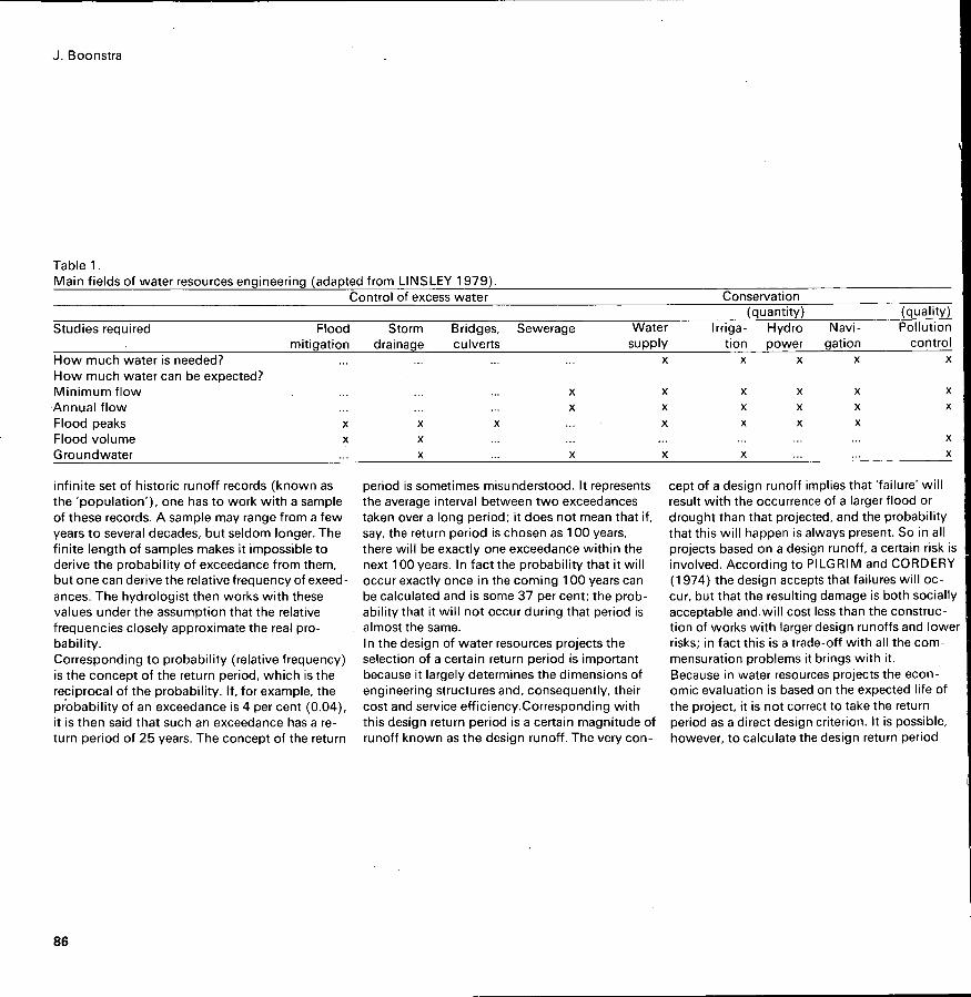
Table 1. Main fields of water resources engineering (adapted from LINSLEY 1979).

Control of excess water Conservation (quantity ) (qua I ity )

Studies required Flood Storm Bridges, Sewerage Water Irriga- Hydro Navi- Pollution mitigation drainage culverts supply tion power gation control

How much water is needed? ... ... ... ... X X X X X

How much water can be expected? Minimum flow ... ... ... X X X X X X

Annual flow ... ... ... X X X X X X

Flood peaks X X X ... X X X X

Flood volume X X ... ... Ground water ... X X X X

... ... ... ... X

... ... ... X

infinite set of historic runoff records (known as the 'population'), one has to work with a sample of these records. A sample may range from a few years to several decades, but seldom longer. The finite length of samples makes it impossible to derive the probability of exceedance from them, but one can derive the relative frequency of exeed. ances. The hydrologist then works with these values under the assumption that the relative frequencies closely approximate the real pro- babi l ity. Corresponding to probability (relative frequency) is the concept of the return period, which is the reciprocal of the probability. If, for example, the probability of an exceedance is 4 per cent (0.04), it is then said that such an exceedance has a return period of 25 years. The concept of the return

period is sometimes misunderstood. It represents the average interval between two exceedances taken over a long period; it does not mean that if, say, the return period is chosen as 1 O0 years, there will be exactly one exceedance within the next 1 O0 years. In fact the probability that it will occur exactly once in the coming 1 O0 years can be calculated and is some 37 per cent; the probability that it will not occur during that period is almost the same. In the design of water resources projects the selection of a certain return period is important because it largely determines the dimensions of engineering structures and, consequently, their cost and service efficiency.Corresponding with this design return period is a certain magnitude of runoff known as the design runoff. The very con-

cept of a design runoff implies that 'failure' will result with the occurrence of a larger flood or drought than that projected, and the probability that this will happen is always present. So in all projects based on a design runoff, a certain risk is involved. According to PILGRIM and CORDERY (1 974) the design accepts that failures will occur, but that the resulting damage is both socially acceptable and will cost less than the construction of works with larger design runoffs and lowei risks; in fact this is a trade-off with all the com- mensuration problems it brings with it. Because in water resources projects the econ- omic evaluation is based on the expected life of the project, it is not correct to take the return period as a direct design criterion. It is possible, however, to calculate the design return period

86

J. Boonstra

ent century, it received an impetus with the introduction of probabilistic methods. Then, in the early 1 930's, because rainfall records are generally longer and more numerous than streamflow records, theoretical hydrologists shifted their at- tention to deterministic (rainfall-runoff) methods, which in their turn led to the development of what are known as component models. That was roughly the state of the art in the late 1950's, when the advent of the digital computer brought a powerful tool to the hydrologist and radically changed the application of mathematical models in surface water hydrology. With its very high rate of arithmetic computation, the computer made it possible to represent time and space variables and to integrate the different processes (components) of the hydrological cycle. Within the deterministic approach, the computer created a new tier- the conceptual model- which is sometimes referred to as a deterministic simulation approach. Introduced into the statistical approach, the computer led to the development of the stochastic model. Most quantitative hydrologic methods can be classified either as deterministic or as statistical. Deterministic methods treat the hydrological processes in a physical way and make use of historical streamflow data as well as data on rainfall and other phenomena (infiltration, evapotranspiration, etc.) which affect the properties of runoff. These methods are called deterministic because,

Figure 3. Methods and models in surface water hydrology (adapted from FLEMING 1975).

once the parameters are determined, deterministic methods always produce the same output from a given input. Statistical methods utilize information from the analysis of historical streamflow data only. Because these methods deal directly with streamflow its characteristics can only be described by the theory of statistics. Among the many classifications that have been made of the available methods is that by FLEMING (1 975). As shown in Figure 3, the Fleming classification, which will be used in this article, subdivides deterministic hydrology into empirical methods and conceptual models, and statistical hydrology into probabilistic methods and stochastic models.

Empirical methods

One of the earliest flood formulas was that devised by Mulvaney in 1851. Today, almost 130

years later, his rational formula is still famous and is still widely used as a method in design. Mulvaney's was the first formula to relate peak flow to rainfall intensity and drainage area. It was followed by a broad class of other empirical methods relating peak flow to similar and other physical characteristics of a drainage basin. VEN TE CHOW (1 962) reviewed a number of these methods. As the era of simple empiricism ended, that of 'modern' hydrology started in the early 1930's, with the work of SHERMAN (1932). Sherman's paper 'Streamflow from rainfall by the unit-graph method' represented a milestone in hydrology. It led to the development of component models, in which the land phase of the hydrologic cycle is broken into components, the major ones being rainfall, infiltration, evapotranspiration, aquifer response, and streamflow routing. The essence of the unit hydrograph concept

deterministic hydrology * statistical hydrology e component

1 synthesis

I m integrated frequency risk

models models I

di rkct semi-di rect indiiect serial I Markov Monte Carlo I I I correlation models method

I I l - 7 I I I I

physical analog hybr id digital models models models models

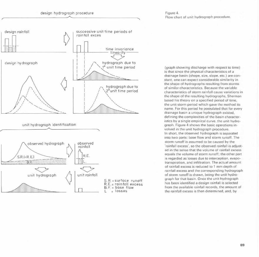
Figure 5. Flow diagram of the Stanford Watershed model (FLEMING 1975).

I

treating this amount of rainfall excess as a con- secutive number of unit storm periods with different intensities and applying the principle of superposition, the design peak discharge is found. The concept of the unit hydrograph has been the subject of many papers; for more information reference is made to LINSLEY (1 967) and DOOGE (1973), who reviewed the literature on the subject. In the 1950's and 1960's the main emphasis in the use of component models was directed towards the problem of identifying unit hydrographs. Classical methods of unit hydrograph derivation were based first on trial and error and secondly on special methods such as the iterative procedure (COLLINS 1939). Modern methods can be classified either as transform methods or as correlation methods. In transform methods computer analysis of hydrographs was attempted on a large scale: NASH (1959) fitted hydrograph shapes to standard probability distributions by multiple regression; O' DONNEL (1960) attempted a similar approach using Fourrier series. In the correlation methods the least squares approach is the basis of the derivation of unit hydrographs. Both SNYDER (1955) and BODY (1 959) expressed the necessary computations in matrix form and developed a program for the digital computer. Both the empirical methods and the unit hydrograph concept are still extensively used; they

_ _ _ _ - _ p&apot ranrp i ra t ion actual \,

I ----/

potential

temperature radiation

A

/?/- impervious

K E Y

(7) [rtotagel

function L I channel

I V I I

I u lower zone upper zone 1 evapotran-

IO- spiration storage depletion I

groundwater storage

channel time delay and routing

1-

I I I I

Solration

have in common that only design flood volumes and design peak discharges can be estimated. For low flow estimates only one method exists, it is based on the theory of groundwater depletion.

Conceptual models

Whereas the component model approach uses discrete time periods, namely only periods of high flows, the conceptual model approach is an integration of the component theories on a con- tinuous time basis, ranging from low to peak discharges. It seeks to simulate catchment behaviour by postulating a certain mathematical operation for each major component of the land

( simulated \ Freamflo-w- I

phase of the hydrological cycle and linking the components together so that the appropriate in- teractions can occur. Because the form of these models depends upon the model-builder's physical concepts of the hydrological cycle, they are also known as conceptual models. In fact, there is no limit to the number of conceptual models that can be devised. The techniques of simulation include: -direct simulation using physical models - semi-direct simulation using analog models - indirect simulation using hybrid and digital

The disadvantage of the first two techniques is that for each drainage basin an entirely new mod-

models

90

peak flow (m3/s 1 10000

5000

2000

1 O00

500

200

1 O0

1.01 1.1 2 10 100 1000 return period (years)

countless papers on the application of probabilistic methods in hydrology have been published. The simplifying assumption made in the probabilistic approach is that the occurrence of an event is assumed to follow a fixed probability distribution. A probability distribution expresses the relationship between the magnitude of an event and the probability of this magnitude being ex ceeded. In probabilistic methods the available

Figure 7. Fitting of two distributions to the annual maxima of the river Styx (PILGRIM and CORDERY 1 974).

data on streamflow are used to f i t a certain frequency distribution, which in turn, in the case of extreme events, is used to extrapolate from the recorded discharges the discharge with the design frequency. Difficulties in probabilistic methods arise from t w o major sources: - the true form of the frequency distribution is not

- sampling errors Numerous different frequency distributions have been used in hydrology, but it is not known to

known

which distribution the discharges can be best fitted. Historical records are much too short to afford any definite empirical evidence. This problem is aggravated by the fact that runoff data can often be fitted wi th satisfactory accuracy to several types of distributions (Figure 7). Goodness of fit tests generally show no significant differences in the fit of the data to the different distributions. However, the tails of the distributions can sometimes be very dissimilar, and these are the probability regions of interest to the designer. Table 2 illustrates the differences in

Table 2. Flood of various frequencies estimated from Fiaure 5 (RILGRIM and CORDERY 1974) - \ , Frequency Period ' Years EstimatLd flood (m3/s) distribution of record 1 O0 vr 1 O00 vr Log normal 1939-66 28 2,4ÓO 6,200 Log Pearson Type Ill 1939-66 28 1,500 3,000

flood discharges of various frequencies estimated from the two distributions. There is no general agreement among hydrologists as to which of the various available theoretical distributions should be used. For example, SPENCE (1973) compared the fit of the normal, 2-parameter lognormal, type I extremal, and log type I extremal distribution to annual maximum flows and found that the lognormal was the best fitting. CRUFF and RANTZ (1 965) compared six frequency distributions and found the Pearson type Ill distribution to be the best, whereas BEN- SON (1 962), in a study of 100 longterm flood records, found that no one type of frequency distributions gave consistently better results than the others. JOSEPH (1 970) studied the probability distribution of annual droughts on 37 stations in the Missouri River basin, U.S.A. Using five distributions, viz. normal, lognormal, square root normal, Weibull and gamma-2 distributions, he arrived at the conclusion that gamma-2 distribution was acceptable for 35 of the 37 stations. In contrast the minimum discharges of the Me- kong River at Vientiane, Laos, were evidently lognormally distributed (MOORE and CLABORN 1971). In short, not a single distribution is acceptable to all hydrologists. Sampling errors, the second major source of dif- ficulty in frequency analysis, relate to estimating the best values of the population parameters once the type of distribution has been selected.

92

lischarge m3/s 150

O0

5 0

O0

5 0

O 1.01 1.1 1.2 13 1.5 2

The magnitude of sampling errors is illustrated by the numerical sampling experiments reported by BENSON (1960). A population of 1000 values fitting a selected frequency distribution was ran- domly divided into samples of various length. Figure 8 reproduces some of the resulting frequency curves of the twenty 50-year samples. Even with a length of 50 years, these results show that large errors are possible and that the frequency curve of recorded floods may be quite different from the true curve of the population.

5 6 7 8 9 1 0 20 30 LO 50 1 O0 return period (years)

NASH and AMOROCHO (1 966) conclude, however, that errors due to sampling variance only coverge towards fixed proportions of the estimates for high return periods. They maintain that, if one could be certain that the assumed form of the probability distribution was correct, magnitudes corresponding to even the very high- est return periods could be estimated with quite tolerable accuracy from even relatively small samples

Figure 8. Frequency curves for 50-year periods (adapted from BENSON 1960).

Stochastic models

Many hydrological sequences exhibit a departure from randomness in that large values tend to be followed by large ones, and small values by small ones, so that runoff values of similar magnitudes tend to persist throughout the sequence. If we are interested in monthly or daily flows, we find that the flow in a particular month or on a particular day will be influenced by the flow(s) of the previous month(s) or day(s), whereas the magnitude of extremes is seldom influenced by the occurrence of previous extremes (trom year to year). Where persistence is present, probabilistic methods cannot be used in planning and design- ing water resources projects. Stochastic modelling is a relative newcomer to the science of hydrology. Some of the concepts of stochastic simulation had been used much earlier, in reservoir design, but widespread application did not begin until the 1960's. The approach in stochastic modelling is to generate long hypothetical sequences of discharges based on the statistical and probability characteristics of the historic records; this approach is also called stochastic simulation, and is comparable to deterministic simulation with conceptual models. As an example, reference is made to a study by O'DONNELL et al. (1 972) who analyzed the flood magnitude-frequency relationship for the river Vardar, Jugoslavia. Using the 42 annual max-

93

1 L O O

1200

600

LOO

0.2

return period (years1 1.25 2 5 10 20 50 100 200 LOO 1000

. 0.6 0.8 0.9 0.95 0.98 0.99 0.9950.99750.999 probability

imum floods, they fitted these events to Gumbel and Fréchet distributions. For the largest annual event in the 42 years of record (1 600 m3/s), widely different return periods of 80 years (Fréchet) and 300 years (Gumbel) were found (Figure ga). They then felt that stochastic simulation would improve the results, because in probabilistic methods only a fraction of the information con- tained in the 42 years of records is used, i.e. one item of data per year. A total of 25 sets of daily data, each set 42 years long, were generated and the annual maximum floods abstracted. Figure 9b shows the generated annual maxima (in excess of 400 m3/s) fitted to the two distributions. It was concluded that the Fréchet distribution ade- quately represents the flood magnitude-frequency relationship for the river Vardar and that the historic flood of 1600 ma/s has a return period of just over 200 years. The procedure in stochastic modelling consists of two parts:

return period (years1

- the choice of a proper model for generating

- the choice of a proper probability distribution

The models used are basically of the Markov or the Monte Carlo type. The difference between the two lies in the treat- ment of the data. The Monte Carlo method considers the data to be totally independent and is concerned with defining the probability distribution from the historic data population and, then using a selected random generating technique to produce the synthetic series of data. The Markov technique is concerned with non- pure random data, i.e. data composed of both causal and random elements. In the Markov lag- one model, for instance, which means that the flow in, say, a particular month is only influenced by the flow in the previous month, the flow is assumed to be the sum of: -the mean flow in that month - a proportion (given by the correlation coeffi-

flows

for the input.

Figure 9. Generation of daily data.

cient) of the departure of the previous flow from its mean

- a random component (residual) The first two components are the statistical part, directly derived from the data, and the third is the stochastic element which is commonly assumed to be either normally, log-normally, or gamma distributed. Markov models were the first stochastic models applied for the generation of streamflow sequences (THOMAS and FIERING 1962; YEV- JEVICH 1963); these models are short-memory models. Since then, there has been an almost ex- plosive growth in the development of models for the generation of synthetic hydrological data sequences. The assumptions implicit in the Markov type models, however, have been challenged (MAN- DELBROT and WALLIS 1968). The consideration of short-term and long-term dependence has led hydrologists and statisticians to propose various alternative models for the stochastic simu lation of hydrologic time series. To preserve very long-term cycles in the streamflow process, the fractional Gaussian noise (FGN) model was developed (MANDELBROT and van NES 1968), and to describe a wide range of behaviour in time series BOX and JENKINS (1970) developed an Autoregressive-integrating-moving average (ARIMA) model. Stochastic simulation can be applied to both

94

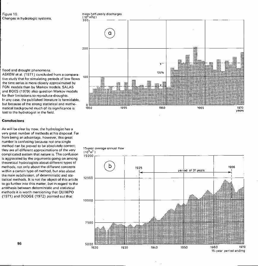
Figure 1 O. Changes in hydrologic systems.

15000

L< 1935

I period of 31 years

I 12500 I

flood and drought phenomena. ASKEW et al. (1 971 ) concluded from a comparative study that for simulating periods of low flows the time series is more closely approximated by FGN-models than by Markov models. S A U S and BOES (1 979) also question Markov models for their limitations to reproduce droughts. In any case, the published literature is formidable, but because of the strong statistical and mathe-

lost to the hydrologist in the field.

Conclusions

i matical background much of its significance is

!

1966

I I

& I 7

As will be clear by now, the hydrologist has a very great number of methods at his disposal. Far from being an advantage, however, this great number is confusing because not one single method can be proved to be absolutely correct; they are all different approximations of the very complicated system that nature is. The confusion is aggravated by the arguments going on among theoretical hydrologists about different types of methods, not only about the different concepts within a certain type of method, but also about the main subdivision, of deterministic and statistical methods. lt is not the object of this article to go further into this matter, but in regard to the antithesis between deterministic and statistical methods it is worth mentioning that QUIMPO (1 971 ) and DOOG E (1 972) pointed out that

95

mean half-yearly discharges ( l o6 m?d 300

ïg50 1955 1960 '1965 1970 years

10000

7 500

5000 1920 1930 19LO 1950 1960 1970

15-year period ending

J. Boonstra

Markov and ARlMA models respectively- both stochastic models- are in principle equivalent to certain types of conceptual models. Although the deterministic and statistical methods have certain basic differences they share two characteristics of primary importance: their dependence on historical records for the values of the parameters and the assumption of time- invariance of the hydrologic systems. The first characteristic means that the results of both these methods are affected by the correct- ness of the historical records. In many instances the records are too short to represent the true distribution of the variables in statistical terms: the historical data record is not a correct sample of the universe of natural events. The second characteristic requires that hydrologic systems must not change in time, relative to their behaviour during the recorded past. In re- ality hydrologic systems change often, either through natural or artifical causes. As an illustra- tion Figure 1 Oa shows a positïve jump of 124 per cent in the mean monthly discharges of'the river Nile, while Figure 1 Ob shows an increase in the 15-year average annual f low of the river Kafue of some 66 per cent. The above considerations have perhaps only aggravated the bewilderment that the hydrologist is facing nowadays. FELDMAN (1 979) concluded that empirical and probabilistic methods may be good for small areas where river routing and stor-

age effects are not significant, but that for larger areas and studies the simulation model is the best tool. There are two main alternatives of flow simulation: - stochastic simulation (without consideration of

- deterministic simulation, starting from simulated

Stochastic simulation can be used if sufficiently long time-series of f low observations are available. In all other cases deterministic simulation must be applied. The fact remains that different methods are available for different purposes. It is therefore of the utmost importance that unbiased criteria and standardization are made available to test all the proposed models and to identify their individual merits and advantages for specific applications. CEMBROWICZ et al. (1 978) analyzed 23 mathematical models dealing with hydrological variables, both deterministic and stochastic. Some of their findings were: - Some of the models, well-knQwn all over the

precipitation)

precipitation

world, were certainly not the best for a particular purpose.

turned out to be most satisfactory for that purpose.

structure requiring detailed input information (up to 166 parameters) which is seldom avail-

- Other models, which are not so well-known,

- Some models revealed a very sophisticated

able. Therefore, less complex models are often more suitable for practical purposes.

The last view is endorsed by the World Meteo- rological Organization (WMO) which published a report in 1975 on the intercomparison of rainfall-runoff models, stating that under certain conditions simple models are as effective as the more elaborate ones. The WMO report also indi- cated the need to develop objective criteria which can be used to compare the performance of the different, existing, models. In summary, it can be stated that the field of hydrological modelling has undergone extensive development, stimulated by the introduction of the digital computer, without which conceptual modelling techniques and stochastic generations of streamflow data would be unthinkable. The fact remains that the gap between theoretical and applied hydrology is still open.

96

Methods and models in surface water hydrology

R E F E R E N C E S

4SKEW, A. J., W. W-G. YEH, and W. A. HALL [I 971 ) . A comparative study of critical drought jimulation. Water Resour. Res. 7, 52-62. 3EN CHlE YEN (1 970). Risk in hydrologic design i f engineering projects. J. Hydraul. Div. 96, 359-966. 3ENSON, M. A. (1 960). Characteristics of frequency curves based on a theoretical 1000-year ,ecord. In: Flood frequency analysis, T. Dal- 'ymple. U.S. Geol. Survey Water Supply Pap.

3ENSON. M. A. (1962). Evolution ofmethodsfor ?valuating the occurrence of floods. U.S. Zeol. Survey Water Supply Pap. 1580-A. 30DY, D. N. (1 959). Flood estimation. Bull. 4, Nater Res. Found. Aust., Sydney. 30X, G. E. P. and G. M. JENKINS (1970). Time series analysis: forecasting and control. dolden-Day Inc., San Francisco. ZEMBROWICZ, R. G., H. H. HAHN, E. J. PLATE, 3nd G. A. SCHULTZ (1978). Aspects of present iydrological and water quality modelling. Eco- logical Modelling 5, 39-66. ZOLLINS, W. T. (1 939). Runoff distribution graphs from precipitation occurring in more than m e time unit. Civil Eng. 9, 55S561. ZRAWFORD, N. H. and R. K. LINSLEY (1966). 3igital simulation in hydrology, Stanford Watershed ModelIV. Tech. Rep. 39. Dept. of Civil

I543-A, 51-77.

Eng., Stanford Univ., California. CRUFF, R. W. and S. E. RANT2 (1965). A comparison of methods used in flood frequency studies for coastal basins in California. U. S. Geol. Survey Water Supply Pap. 1580-E. DOOGE, J. C. I. (1972). Mathematical models of hydrologic systems. In: Proc. Int. Symp. on modelling techniques in water resources systems. Ottawa, 171-1 89. DOOGE, J. C. I. (1973). Thelineartheoryof hydrologic systems. U.S. Dept. of Agric., Tech. Bull. 1468, U.S. Govt. Printing office, Washington D.C. FELDMAN, A. D. (1979). Comparison of techniques for determining flood frequency relation ships. Paper presented at the Int. Symp. on Spe- cific Aspects of Hydrological Computations for Water Projects, Leningrad, U.S.S.R. FLEMING, G. (1975). Computer simulation techniques in hydrology. Elsevier, New York. FLEMING, G. (1979). Deterministicmodelsin hydrology. FAO Irrig. Drain. Pap. 32, Rome. FULLER, W. E. (1914). Floodsflows. Trans. Am. Soc. Civil Eng. 77, 5 6 5 6 1 7. JOSEPH, E. S. (1 970). Probability distribution of annual droughts. J. lrrig. Drain. Div. 96, 461-474. LINSLEY, R. K. (1 967). The relation between rainfall and runoff. J. Hydrol. 5, 297-31 1. LINSLEY, R . K. and J. B. FRANZlNl (1 979). Water resources engineering. McGraw-Hill, New York.

MANDELBROT, B. B. and J. R. WALLIS (1 968). Noah, Joseph, and operational hydrology. Water Resour. Res. 4, 909-91 8. MANDELBROT, B. B. and J. W. van NES (1968). Fractional Brownian motions, fractional noises and applications. Rev. Soc. lnd. Appl. Math. 70, 422-437. MOORE, W. L. and B. J. CLABORN (1971). Numerical simulation of watershed hydrology. In: Proc. 1st U.S. -Japan Bilateral Semin. in Hy- drology, Honolulu, Hawaii. NASH, J.E. (1 959). Systematic determination of unit hydrograph parameters. J. Geophys. Res. 64, 11 1-1 15. NASH, J. E. and J. AMOROCHO (1966). The accuracy of the prediction of floods of high return periods. Water Resour. Res. 2, 191-1 98. O'DONNEL, T. (1960). Instantaneous unit hy- drographderivation by harmonicanalysis. Publ. 57, Int. Assoc. Sci. Hydrol.. 546-557. O'DONNEL, T., M. J. HALLand P. E. O'CONNELL (1972). Some applications of stochastic hydrological models. In: Proc. Int. Symp. on Modelling Techniques in Water Resources Systems, Ottawa, Canada. OTT, R. F. (1 971). Streamflow frequency using stochastically generated, hourly rainfall. Tech. Rep. 151. Dept. of Civil Eng., Stanford Univ., California. PILGRIM, D. H. and I. CORDERY (1974). Design flood estimation; an appraisal of philos-

97

J. Boonstra

ophies and needs. Water Res. Lab. Rep. 140, Manly Vale, Australia. QUIMPO, R. G. (1971). Kernelsof stochastic linear hydrologic systems. In: Proc. 1st U.S.- Japan BilateralSemin. in Hydrology, Honolulu, Hawaii. SALAS, J. D. and D. C. BOES (1979). Appli- cation of shifting level models for operational hydrology. Paper presented at the Int. Symp. on Specific Aspects of Hydrological Computations for Water Projects, Leningrad, U.S.S.R. SHERMAN, L. K. (1932). Streamflow from rainfall by the unit-graph method. i n g . News Record 108,501-505. SNYDER, W. M. (1955). Hydrograph analysis by the method of least squares. In: Proc. Am. Soc. Civil. Eng. 81. Separate 793. SPENCE, E. S. (1 973). Theoretical frequency distributions for the analysis of plains streamflow, Can. J . Earth Sci. 1 O, 130-1 39. THOMAS, H. A. and M. B. FIERING (1962). Mathematical synthesis of streamflow sequences for the analysis of river basins by simulation. In: Design of water resources systems, A. MAASS et al., Harvard Univ. Press, 459-493. VEN TE CHOW (1 962). Hydrologicdetermina- tion of waterway areas for the design of drainage structures in small drainage basins. Eng . Expt. St. Bull. 462, Univ. of :Ilinois. W M O (1 975). Intercomparison of conceptual models used in operational hydrological forecast-

ing. WMO Operational Hydrol. Rep. 7, Geneva. YEVJEVICH, V. (1963). Fluctuations of wet and dry years. Part I, Research data assembly and mathematical models. Hydrol. Pap. 1, Colorado State Univ., Fort Collins.

98

methods and models in surface water hydrology · one of these is water resources engi- ... the role...

Documents