methods for estimating odor emissions scott...

METHODS FOR ESTIMATING ODOR EMISSIONS

By Chester M. Morton, P.E., Scott Tudman

Malcolm Pirnie, Inc. 104 Corporate Park Drive White Plains, NY 10602

ABSTRACT The emission and control of odors from wastewater facilities is receiving increasing attention by citizens who reside in the communities surrounding these facilities, the municipal agencies responsible to build and operate them, and from the regulators whose job it is to ensure they are operated within their operating permits. Odorous compounds associated with wastewater are listed, including their odor threshold and detection concentrations, and odor description. The odor threshold values of volatile organic compounds (VOCs) are also presented. Air emission measurement techniques that are used to develop emissions rates are described. Air sample collection methods and different analytical methods used to characterize odorous air samples are discussed which include: sensory analysis and odor measurement; chemical analysis to identify compounds; portable and handheld equipment with data logging capabilities, and optical remote sensing. Liquid phase analyses that are normally conducted as part of an odor survey are reviewed. KEYWORDS Odor, Dilution-to-Threshold, D/T, hydrogen sulfide, reduced sulfur, emission estimation INTRODUCTION The emission and control of odors from wastewater facilities is receiving increasing attention by citizens who reside in the communities surrounding these facilities, municipal agencies responsible to build and operate them, and from the regulators whose job it is to ensure they are operated within their operating permits. Although selected States and communities include in their odor regulations, odor strength and hydrogen sulfide concentrations, most focus on nuisance terms, or are based on the interference of “quality of life.” Despite the lack of numerical limits, many municipalities recognize the need to control odors and to be a good neighbor. As a result, substantial resources are devoted to identifying, measuring and controlling odors, and unfortunately in some instances, litigating cases where odors have not been adequately controlled. The origin of this paper is a project Malcolm Pirnie is conducting for a large municipality that is re-evaluating its methodology of measuring and regulating odor emissions.

Odors and Toxic Air Emissions 2002

Copyright © 2002 Water Environment Federation. All Rights Reserved.

The first step in addressing odor emissions, whether it be for monitoring or control, is their measurement. The methods used to sample and analyze odors in order to estimate odor emissions from wastewater facilities are described. The emission estimates are used to conduct dispersion modeling to determine offsite impacts, and in the design of odor control systems. First, the odor recognition and detection thresholds of compounds associated with wastewater facilities are reported. The odor threshold values of volatile organic compounds (VOCs) are presented. The advantages and disadvantages of indirect and direct measurements are evaluated. The use of emission isolation flux chambers and exhaust air stream sampling to estimate emissions is discussed. Air sample collection methods including whole air sampling, and adsorption/absorption using sorbents and solutions are described. The following topics associated with analytical parameters and methods that are used to characterize air samples are discussed:

• Sensory analysis which includes the parameters: odor strength (dilution-to-

threshold), intensity, descriptors, and dose-response, also referred to as persistence.

• The current development of an international standard for olfactometry. • Chemical analysis of odor constituents by gas chromatography, conversion to

total reduced sulfur and the use of various detectors including pulsed florescence, chemiluminescence, and flame photometric detectors.

• Advantages and disadvantages of portable and held-held devices including Jerome meters, Interscans, Thermal Environmental Instruments, and Zellweger chemcassette devices.

• Monitoring devices with data logging. • Analyzing the wastewater as part of an odor survey, and the parameters analyzed.

ODOROUS COMPOUNDS The range of odors emitted by wastewater collection and treatment systems is limited only by the range of natural, man-made and manufactured materials that are discharged to the these systems, and the metabolic by-products of the microbes which consume the varied diet man supplies them. The perception of odors is accomplished through the olfactory system that includes the sensing organ in the nose, the olfactory epithelium. The olfactory epithelium includes approximately one million receptor cells. The receptor cells connect to the olfactory bulb located behind the eyes, above the nasal chamber, in the lower front part of the brain. The receptor cells react with the chemical/ physical properties and molecular characteristics of odorous substances to produce stimuli that is recognized as an odor. The trigeminal nerve is also part of the olfactory system and initiates protective reflexes. The olfactory system is complex and individual responses to odors is variable, which results in a variation in the detection levels of odorants. (McGinley et al April 2000, WEF MOP No. 22)



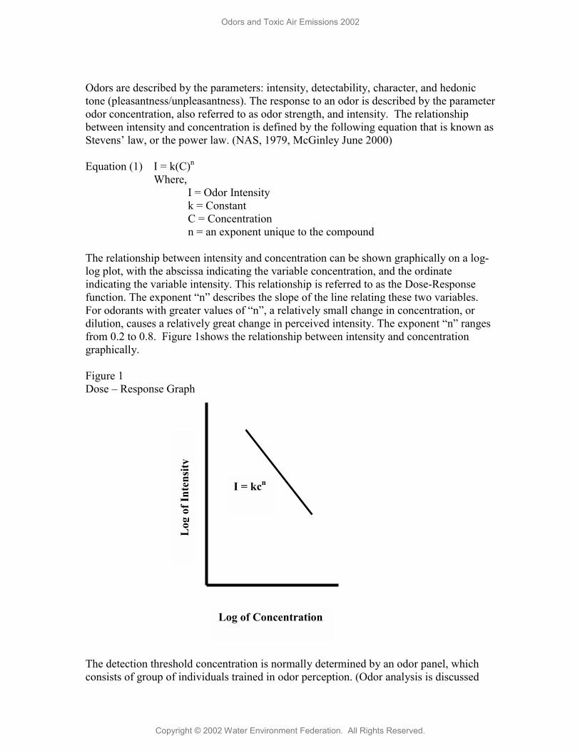
Odors are described by the parameters: intensity, detectability, character, and hedonic tone (pleasantness/unpleasantness). The response to an odor is described by the parameter odor concentration, also referred to as odor strength, and intensity. The relationship between intensity and concentration is defined by the following equation that is known as Stevens’ law, or the power law. (NAS, 1979, McGinley June 2000) Equation (1) I = k(C)n

Where, I = Odor Intensity k = Constant C = Concentration n = an exponent unique to the compound

The relationship between intensity and concentration can be shown graphically on a log-log plot, with the abscissa indicating the variable concentration, and the ordinate indicating the variable intensity. This relationship is referred to as the Dose-Response function. The exponent “n” describes the slope of the line relating these two variables. For odorants with greater values of “n”, a relatively small change in concentration, or dilution, causes a relatively great change in perceived intensity. The exponent “n” ranges from 0.2 to 0.8. Figure 1shows the relationship between intensity and concentration graphically. Figure 1 Dose – Response Graph The detection threshold concentration is normally determined by an odor panel, which consists of group of individuals trained in odor perception. (Odor analysis is discussed

Log

of I

nten

sity

Log of Concentration

I = kcn



further in the paragraphs below.) Odors are presented to the panel through the use of an olfactometer. Samples of odorous air are presented to the odor panel members at increasing concentrations by decreasing the volume of clean filtered dilution air, also referred to as “zero air”, that is added to an odorous air sample. The detection threshold concentration is defined as the concentration at which 50% of the panel members detect an odor. The recognition threshold is the concentration at which the character of an odor can be recognized. The recognition threshold is typically 2 to 10 times the detection threshold (Dravnieks 1980).

The detection threshold for a compound will vary depending on the sensitivity of the panelists, the olfactometer design that is used to present the odorous air to the panelist, and the flow rate of air that is used to present the odor sample to the panelist. There is a standard protocol for odor measurement (ASTM 679-91), but there has been variability in the design of the olfactometer used by different odor laboratories. Odor threshold concentrations reported in the literature may vary by a factor of 10 or more. This is believed to be the result of inconsistent methods between the laboratories that conducted the evaluations, variation in olfactometer design, too few odor panel members, and/or too large a change in odorant concentration when conducting the tests. (Dravnieks 1980, WEF MOP No. 22) Hydrogen sulfide has published odor thresholds varying from 1-ppb to 130-ppb (AIHA, 1989).

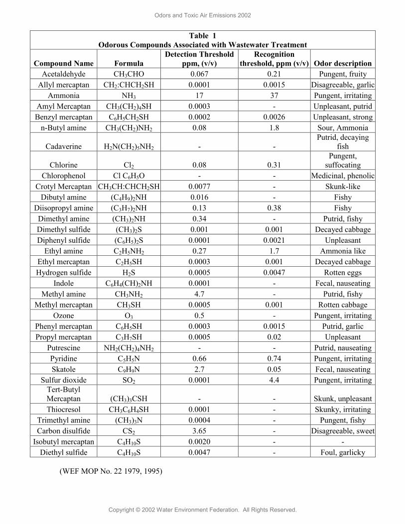
Table 1 lists the detection and recognition thresholds, and odor descriptors for odorous compounds associated with wastewater. The sulfur containing compounds have the lowest detection threshold except for trimethyl amine. Hydrogen sulfide is the most common odorous compound associated with wastewater, but it should not be assumed that an odor problem is caused exclusively by hydrogen sulfide. Table 2 lists the odor thresholds for volatile organic compounds (VOCs) associated with wastewater. In most cases the odor threshold value for these VOCs are well above their measured concentration at wastewater treatment plants. AIR EMISSION MEASUREMENT Air emission measurement techniques can be categorized into two different types of approaches, direct and indirect emission measurement techniques. Direct measurement techniques consist of isolating all or a portion of an emission source by using an enclosure or specially designed chamber. The concentration of emissions emitted from the isolated space or surface is measured by collecting samples using equipment unique to the parameter(s) of interest, or, depending on the parameter being measured, real-time measurements can be taken which enable decision-making during the emission measurement effort. The concentration measurements, along with other parameters, are then used to calculate an emission flux. The emission flux can then be related to an emission rate for the entire source. The emission rates that are generated can be used in dispersion models to predict ambient air concentrations under various meteorological conditions.



Indirect measurement approaches generally consist of measuring the ambient air concentration of the emitted species and then applying these data to an equation i.e., an air dispersion model, to determine the emission rate. The methodology used in most of the indirect approaches is similar and involves ambient air samplers located upwind and downwind of the emission source. Meteorological conditions are also required because the various dispersion models used to calculate the emission flux require wind speed and temperature values. Some methods require extensive sampler arrays. One limitation of these approaches is that the meteorological conditions during the sampling effort match the conditions on which the sampler locations were selected.

Direct measurement methods are the preferred approach because they have been proven to be relatively cost-effective in obtaining concentration data and in determining emission rates, and preclude the need to conduct modeling to develop emission rates. As a result only direct measurement approaches are described in this paper. Readers are referred to the literature for information about indirect measurement approaches (USEPA, 1990).

Emission Isolation Flux Chamber The most commonly used direct measurement device is the isolation flux chamber which isolates a known surface area for emission flux measurement. Emissions enter from the bottom of the chamber from the surface being sampled, and clean, dry sweep air is added at a metered rate. The sweep air is mixed with emitted vapors and gases by the physical design of the sweep air inlet. “The sweep air creates a slight wind velocity at the emitting surface, preventing a build-up of the emissions concentration in the boundary layer directly above the surface. The exit port is used for the measurement of the concentration of air within the chamber or for sampling and analysis. A pressure relief port in the enclosure, which prevents pressure build-up within the chamber that may otherwise occur while sampling liquid surfaces.” On water surfaces, a support or flotation device is necessary. (USEPA 1990)

This technique directly measures an instantaneous emission flux from the surface being sampled. The emission flux is calculated from the surface area isolated, the sweep air flow rate, and the emission concentration.

The emission isolation flux chamber was validated for EPA for measuring volatile emissions from landfills, however, it is applicable to emission flux measurement from all types of area sources, such as lagoons, landfills, open dumps, and waste piles. The flux chamber validated for EPA has a diameter of 16-inches, a skirt height of 7-inches and a height from the bottom of its skirt to the top its cover of 11-inches. A comprehensive description of its use, schematic diagram, and specifications is contained in the Flux Chamber User’s Guide (USEPA 1986).



(WEF MOP No. 22 1979, 1995)

Table 1 Odorous Compounds Associated with Wastewater Treatment

Compound Name Formula Detection Threshold

ppm, (v/v) Recognition

threshold, ppm (v/v) Odor descriptionAcetaldehyde CH3CHO 0.067 0.21 Pungent, fruity

Allyl mercaptan CH2:CHCH2SH 0.0001 0.0015 Disagreeable, garlicAmmonia NH3 17 37 Pungent, irritating

Amyl Mercaptan CH3(CH2)4SH 0.0003 - Unpleasant, putridBenzyl mercaptan C6H5CH2SH 0.0002 0.0026 Unpleasant, strong

n-Butyl amine CH3(CH2)NH2 0.08 1.8 Sour, Ammonia

Cadaverine H2N(CH2)5NH2 - - Putrid, decaying

fish

Chlorine Cl2 0.08 0.31 Pungent,

suffocating Chlorophenol Cl C6H5O - - Medicinal, phenolic

Crotyl Mercaptan CH3CH:CHCH2SH 0.0077 - Skunk-like Dibutyl amine (C4H9)2NH 0.016 - Fishy

Diisopropyl amine (C3H7)2NH 0.13 0.38 Fishy Dimethyl amine (CH3)2NH 0.34 - Putrid, fishy Dimethyl sulfide (CH3)2S 0.001 0.001 Decayed cabbage Diphenyl sulfide (C6H5)2S 0.0001 0.0021 Unpleasant

Ethyl amine C2H5NH2 0.27 1.7 Ammonia like Ethyl mercaptan C2H5SH 0.0003 0.001 Decayed cabbage Hydrogen sulfide H2S 0.0005 0.0047 Rotten eggs

Indole C6H4(CH)2NH 0.0001 - Fecal, nauseating Methyl amine CH3NH2 4.7 - Putrid, fishy

Methyl mercaptan CH3SH 0.0005 0.001 Rotten cabbage Ozone O3 0.5 - Pungent, irritating

Phenyl mercaptan C6H5SH 0.0003 0.0015 Putrid, garlic Propyl mercaptan C3H7SH 0.0005 0.02 Unpleasant

Putrescine NH2(CH2)4NH2 - - Putrid, nauseatingPyridine C5H5N 0.66 0.74 Pungent, irritatingSkatole C9H9N 2.7 0.05 Fecal, nauseating

Sulfur dioxide SO2 0.0001 4.4 Pungent, irritatingTert-Butyl Mercaptan (CH3)3CSH - - Skunk, unpleasantThiocresol CH3C6H4SH 0.0001 - Skunky, irritating

Trimethyl amine (CH3)3N 0.0004 - Pungent, fishy Carbon disulfide CS2 3.65 - Disagreeable, sweet

Isobutyl mercaptan C4H10S 0.0020 - - Diethyl sulfide C4H10S 0.0047 - Foul, garlicky



T

AB

LE 2

V

olat

ile O

rgan

ic C

arbo

n C

ompo

und

Odo

r T

hres

hold

s R

uth

Am

. Ind

. Hyg

. Ass

oc.

mg/

m3

ppm

pp

m

ppm

A

ccep

tabl

e V

alue

s A

ll V

alue

s (pp

m)

C

ompo

und

M

ol w

t. g/

mol

Lo

w

Hig

h Lo

w

Hig

h T

hres

hold

lim

it va

lue

(TLV

)

Ty

pe o

f th

resh

old

Geo

M

ean

Low

(p

pm)

Hig

h (p

pm)

Low

H

igh

100

TWA

de

tect

ion

160

160

* 1.

2 44

0 M

ethy

lene

chl

orid

e 84

.94

540

2,16

0 15

3 61

0

re

cogn

ition

23

0 23

0 *

Chl

orof

orm

11

9.39

25

0 10

00

50

201

10

TWA

de

tect

ion

192

133

276

0.6

1,41

3 35

0 TW

A

dete

ctio

n 39

0 --

- --

- 16

71

4 1,

1,1-

Tric

hlor

oeth

ane

133.

41

N/A

N

/A

N/A

N

/A45

0 ST

EL

reco

gniti

on

710

---

---

---

---

dete

ctio

nF 25

2 14

0 58

4 1.

6 70

6 C

arbo

n Te

trach

lorid

e 15

3.82

30

0 50

0 47

78

5

TWA

re

cogn

ition

F 25

0 25

0 *

---

---

dete

ctio

n N

/A

---

---

---

---

1,1-

Dic

hlor

oeth

ene

96.9

438

0.33

58

1975

0.

08

489

N/A

N

/A

reco

gniti

on

N/A

--

- --

- --

- --

- 50

TW

A

dete

ctio

n 82

82

*

0.5

167

Tric

hlor

oeth

ylen

e 13

1.39

1.

13

2,16

0 0.

21

395

200

STEL

re

cogn

ition

11

0 11

0 *

---

---

50

TWA

de

tect

ion

no

ne

none

2

71

Tetra

chlo

roet

hyle

ne

165.

83

32

469

4.6

68

200

STEL

re

cogn

ition

---

---

---

---

Chl

orob

enze

ne

112.

56

0.98

28

0 0

60

75

TWA

de

tect

ion

1.3

1.3

0.

087

5.9

Vin

yl C

hlor

ide

62.5

0 N

/A

N/A

N

/A

N/A

5 TW

A

N

one

none

no

ne

10

20

O-D

ichl

orob

enze

ne

147.

00

12

300

2 49

50

TW

A

dete

ctio

n 0.

7 0.

7 *

0.02

50

M

-Dic

hlor

oben

zene

14

7.00

N

/A

N/A

N

/A

N/A

N/A

N

/A

N/A

N

/A

---

---

---

---

P-D

ichl

orob

enze

ne

147.

00

90

180

15

29

75

TWA

de

tect

ion

0.12

0.

12

* <1

5

200

TWA

de

tect

ion

Non

e no

ne

49

13

59

1,1-

Dic

hlor

oeth

ane

98.9

6 44

5.5

810

108

196

250

STEL

re

cogn

ition

N

/A

---

---

---

---

10

TWA

de

tect

ion

26

6 11

1 4.

3 68

0 1,

2-D

ichl

oroe

than

e 98

.96

445.

5 81

0 10

8 19

6 N

/A

STEL

re

cogn

ition

87

41

18

5

10

TW

A

dete

ctio

n 61

34

11

9 0.

78

160

Ben

zene

78

.11

4.5

270

1.4

83

N/A

ST

EL

reco

gniti

on

97

*

100

TWA

de

tect

ion

1.6

0.16

37

0.

021

69

Tolu

ene

92.1

4 8.

02

150

2.1

39

150

STEL

re

cogn

ition

11

1.

9 69

Et

hyl b

enze

ne

106.

16

8.7

870

2.0

197

100

TWA

de

tect

ion

none

N

/A

N/A

0.

092

0.6

Odo

rs a

nd T

oxic

Air

Em

issi

ons

2002

Cop

yrig

ht ©

200

2 W

ater

Env

ironm

ent F

eder

atio

n. A

ll R

ight

s R

eser

ved.

TA

BLE

2

Vol

atile

Org

anic

Car

bon

Com

poun

d O

dor

Thr

esho

lds

Rut

h A

m. I

nd. H

yg. A

ssoc

. m

g/m

3 pp

m

ppm

pp

m

Acc

epta

ble

Val

ues

All

Val

ues (

ppm

)

Com

poun

d

M

ol w

t. g/

mol

Lo

w

Hig

h Lo

w

Hig

h T

hres

hold

lim

it va

lue

(TLV

)

Ty

pe o

f th

resh

old

Geo

M

ean

Low

(p

pm)

Hig

h (p

pm)

Low

H

igh

125

STEL

re

cogn

ition

--

- --

- --

- --

- --

- O

-Xyl

ene

106.

20

0.34

17

0 0.

08

38

---

---

dete

ctio

n 0.

62

0.62

*

0.08

1 0.

55

Met

hyl-t

ert-b

utyl

-eth

er88

.15

0.00

0

40

TWA

de

tect

ion

1160

11

60

* <4

0 11

61

Ace

toni

trile

41

.05

70

70

41

41

60

STEL

re

cogn

ition

--

- --

--

----

--

- --

- Fr

eon

11

(CC

L3F)

13

7.37

28

11

70.4

5 20

4 N

/A

N/A

N

/A

N/A

--

- --

- --

- --

- 1,

2-D

ibro

mom

etha

ne

173.

83

N/A

N

/A

N/A

N

/AN

/A

N/A

N

/A

N/A

--

- --

- --

- --

- 10

TW

A

dete

ctio

n 0.

45

0.45

*

0.09

9 76

1,

3-B

utad

iene

54

.09

0.35

2 2.

86

0.2

1.3

N/A

ST

EL

reco

gniti

on

1.1

1.1

* --

- --

- ci

s-1,

2-D

ichl

oroe

thyl

ene

96.9

4 0.

3358

19

75

0 48

9 N

/A

TWA

re

cogn

ition

1.

1 1.

1 *

---

---

Ben

zyl c

hlor

ide

126.

59

0.23

5 1.

55

0.04

0.

291

TWA

de

tect

ion

0.04

1 0.

041

* 0.

041

0.04

6 M

+p-X

ylen

e 10

6.20

0.

34

170

0 38

N

/A

STEL

de

tect

ion

0.

062

2.1

0.08

1 0.

12

10

TWA

de

tect

ion

0.00

94

0.00

1 0.

13

0.00

007

1.4

Hyd

roge

n Su

lfide

34

.08

0.00

07

0.01

4 0.

0005

0.

010

15

STEL

re

cogn

ition

0.

0045

*

* --

--

---

N/A

TW

A

dete

ctio

n N

/A

---

----

--

--

---

Thio

phen

e 84

.13

0.00

26

0.00

260.

0007

0.

00N

/A

STEL

re

cogn

ition

N

/A

---

----

--

--

---

N/A

TW

A

dete

ctio

n 0.

001

0.00

73

0.00

1 0.

0041

4.9

N-b

utyl

mer

capt

an

90.1

8 0.

0016

0.

0033

0.00

04

0.00

N/A

ST

EL

reco

gniti

on

0.00

73

---

---

---

---

N/A

TW

A

dete

ctio

n N

/A

---

---

---

---

Dim

ethy

l dis

ulfid

e 94

.19

0.00

01

0.34

650.

0000

3 0.

09N

/A

STEL

re

cogn

ition

N

/A

---

---

---

---

N/A

TW

A

dete

ctio

n N

/A

---

---

---

---

Die

thyl

dis

ulfid

e 12

2.24

0.

0195

0.

0195

0.00

383

0.00

N/A

ST

EL

reco

gniti

on

N/A

--

- --

- --

- --

- N

/A

TWA

de

tect

ion

N/A

--

- --

- --

- >1

0 M

ethy

l chl

orid

e 50

.49

21.0

0 21

.00

10.0

3 10

.03

N/A

ST

EL

reco

gniti

on

N/A

--

- --

- --

- --

- N

/A

TWA

de

tect

ion

160

* *

16

714

1,1,

1, T

richl

oroe

than

e 13

3.42

N

/A

N/A

N

/A

N/A

N/A

ST

EL

reco

gniti

on

690

* *

---

---

Not

es:

STEL

= S

hort

Term

Exp

osur

e TW

A =

Tim

e W

eigh

ted

Ave

rage

*

= Si

ngle

Acc

epta

ble

Val

ue

Odo

rs a

nd T

oxic

Air

Em

issi

ons

2002

Cop

yrig

ht ©

200

2 W

ater

Env

ironm

ent F

eder

atio

n. A

ll R

ight

s R

eser

ved.

This technique does not assess the effects of wind speed on the emission rate, and is not suited to large emission sources with a large degree of heterogeneity. It is not applicable to the measurement of particulate emission fluxes. Also, “the emission fluxes of volatile species may be enhanced or suppressed since the flux chamber alters the environmental conditions at the sampling locations” (USEPA, 1990). Vent Sampling “Vent sampling is performed when an emission source contains vents with measurable flow rates.” This sampling technique requires measuring the emission concentration and the volumetric flow rate, usually as the product of the exhaust velocity and cross-sectional area of the vent. Examples of where vent sampling would apply is a tank vent; an enclosed space containing equipment such as a headworks building; and the discharge of an air phase odor control unit such as a wet scrubber. Vent sampling is not applicable when the vent has minimal or no flow (USEPA, 1990).

Portable Wind Tunnels Wind tunnels are used to directly measure the emission rate of volatile compounds and erodible material. Measurements can be made under varying wind conditions to examine the effect of wind speed on emissions. The equipment consists of portable, open bottomed enclosures used to isolate a known surface area, a blower used to simulate wind conditions, and sampling devices.

Wind tunnels are applicable to emissions measurements from all forms of liquid and solid-area sources. They can be used on clarifiers, and on landfills.

The portable wind tunnels do not account for macro-atmospheric effects on the emission flux. Repeated measurement at a given location, whether it be a tank or landfill, may deplete the mass of volatile materials (USEPA, 1990).

Head Space Samplers Head space samplers can be used as a chamber to isolate part of the emission source surface. The quantity or concentration of vapors and/or gas emitted from the surface that build up in the chamber over a period of time is measured, rather than measuring a specific rate. The headspace sampler is the predecessor to the isolation flux chamber and no validation of this device has been reported.

The samplers can be operated in either static or dynamic modes. “In the static mode, the sampling enclosure is placed over the emitting surface for a given period of time.” Surface emissions enter the chamber and are given time to concentrate before a sample is taken.



The sensitivity of the method is improved due to the buildup of gas species within the chamber. However, the accuracy of the calculated emission rate is dependent on the duration of sampling relative to the time required to reach steady-state concentrations within the chamber. Also, instantaneous changes to the flux cannot be measured.

In the dynamic mode, the sampling enclosure is placed over the emitting surface for a given time period, and collected emissions are continuously withdrawn from the chamber. The chamber can be operated with a second port, which allows ambient air to enter the chamber and thus prevent the buildup of negative pressure.

The advantage of the dynamic mode is that the sampling duration and air sampling rate can be varied to adjust the volume of air sampled so as to achieve the required analytical sensitivities. Also, another advantage is that the method is very simple, and independent of meteorological conditions.

One disadvantage is that as the atmosphere within the enclosure is withdrawn, the emission flux may be affected. This can occur by the addition of bulk flow of the soil gas into the chamber, or by air entrainment occurring within the enclosure because of leakage at the enclosure’s bottom edge.

This technique does not assess the effects of wind speed on the emission flux. For water surfaces, removal of air from the chamber will induce a pressure change unless make-up air is able to enter the chamber. The chamber will require some sort of flotation device, though this may be affected by waves and agitation. Head Space samplers are not applicable to the measurement of particulate emissions fluxes (USEPA, 1990).

Head Space Bottle Samplers Head space analysis of bottled samples is a technique for determining the emission potential of solid materials such as sludges, soils and solid waste. The subject material is collected and is immediately placed in a sampling container (typically a 1 liter or 40 ml vial with septa) and the container is sealed. It is important to transfer the material immediately after collection into the sample container to prevent loss of volatiles. The container is allowed to sit for a certain amount of time (usually 5-30 minutes), after which the container lid is cracked open, and the probe of a field instrument is inserted to determine if vapors are present. Typical field instruments include flame ionization detectors, photoionization detectors, combustion meters, and colorimetric tubes.

Another type of headspace analysis involves analyzing the headspace gas or extracted solids of a waste core. An undisturbed core is collected using an auger. The sample is then sealed in a sample container with minimal headspace. Headspace gas is removed from the core using a syringe and analyzed using a gas chromatograph.



This technique is best suited for measuring adsorbed organics, but it can also be effective with free organics in the pore space if the material is rapidly transferred to the sample container, or if the tube or core sampler is used.

This technique identifies materials which are a potential source of air emissions but does not provide for calculation of an emission rate. Species specific data can be obtained if the proper analytical tools are used, but generally this technique only provides qualitative data (USEPA, 1990). AIR SAMPLE COLLECTION There are three general types of air sampling approaches: whole air sampling where an air sample is collected in a container; pulling the sample air through a sorbent; and bubbling an air sample through a solution which absorbs the compounds to be analyzed. The parameter that is to be analyzed determines the sampling approach. It is the authors’ experience that whole air sampling is most often used and is discussed in more detail below. Sampling through the use of a sorbent or an absorbing solution are similar because the parameters that are to be analyzed are retained on, or in, a medium. These approaches are suited to compounds that are reactive, such as nitrogen groups (ammonia or amines), and others. An air pump is used move the sample air from its source through the sorbent or absorbing solution. The sample pump air flow rate and the duration of sample effort is monitored so that a total air volume can be calculated. By dividing the mass of the compound retained, by the air volume that is passed through the medium, the concentration of the compound is calculated. In some instances passing a greater volume of air through the medium can lower the detection level for a compound. The compounds that are to be analyzed are removed from the sorbent by thermal desorption and solvent extraction. The analytical method for the compound(s) of concern typically call-out the sample medium that should be used. Whole air sampling is the collection of an air sample into a container for the purpose of analyzing the sample for contaminants. There are two basic types of containers available for air sampling: bags and canisters. Bags are available in different materials including Tedlar®, Teflon®, and Mylar and range in size from 0.5 liters to 100 liters. Canisters range from 0.1 liters to 6 liters in size. They are made of stainless steel and may be glass-lined to maintain sample integrity. The type of bag or canister used will depend on the contaminants in the air being sampled. When sampling with bags, a pump must be used to collect the sample. However, care must be taken so that the sample is not contaminated by the pump. This can be accomplished by using a hand pump and an evacuation chamber. The sample bag is placed inside the evacuation chamber, and the bag’s sample valve is connected to a tube



fitting on the evacuation chamber. A sample tube is run from the tube fitting on the evacuation chamber to the odor source that is to be sampled. The pump exhausts the air from the evacuation chamber, causing a vacuum to be present. The vacuum in the evacuation chamber causes a sample to be drawn into the sample bag. The sample bag should be purged with the sample source prior to collecting the sample to avoid excessive sample loss due to adsorption or reaction on the inner surface of the bag. Amongst the three types of bags available, Tedlar® has been shown to be the most reliable in maintaining sample integrity. Even so, samples should be analyzed within 24 to 72 hours depending on the contaminant. Bags should not be used if measuring for trace compounds. Canisters are evacuated causing a negative pressure to be present so sampling is passive. An air sample is drawn into a canister by opening a valve on the canister. Grab samples can be collected over a short period of time by opening the canister valve. Samples can be collected over extended periods of time through the use of flow controllers which allow a canister to be filled at a predetermined rate. Canisters can hold samples several days and still maintain sample integrity. AIR ANALYSIS The analyses that are to be conducted as part of an odor survey will depend on the purpose and scope of the project at hand. Analyzing for odor concentration would be required when ranking odor sources and determining offsite impacts through dispersion modeling. Speciation of the odor causing compounds is valuable when selecting and designing odor control systems. However, in some cases the odor causing compounds cannot be identified and control technologies are selected and designed by evaluating the performance of different control technologies in bench tests and their ability to reduce odor concentration (Morton et al, 1997). In addition, carbon dioxide is often analyzed as part of an odor characterization effort where odor control is expected to be required. This is because carbon dioxide which is non-odorous, is an acid gas that exerts an alkali demand in wet scrubbers. Its concentration could significantly impact operating costs and could affect the selection of an odor control technology. The following paragraphs briefly describe the analytical methods used to characterize odorous air streams in the following categories:

• Sensory analysis and odor measurement • Chemical analysis to identify specific compounds • Chemical analysis using handheld, or portable analytical equipment

The analytical method for the compound(s) of concern typically call-out the sample medium that should be used.



Sensory Analysis and Odor Measurement Odor Concentration. Odorous air is a complex mixture of volatile compounds that together cause a psychophysical response in the olfactory system. Odor sensory analysis determines the odor concentration of an air sample in addition to other odor parameters. Odor concentration is also referred to as Dilution-to-Threshold (D/T) ratio. It is a dimensionless ratio of the final volume of a diluted air sample (V) divided by the initial air sample volume (v), Z = V/v. Numerically Z is equal to odor units per cubic meter. The D/T of an air sample is also referred to as ED50, or, the effective dosage (dilution) at which 50% of an odor panel detects the sample. (Dravnieks, 1980)

There are two methods for determining the odor concentration of an air sample, the static method and dynamic method. The static method is described in ASTM D 1391, whose last revision is dated 1978, and was withdrawn for use by the ASTM E-18 Committee in 1985. In this method, a 100-ml syringe is used to dilute an air sample. The sample is then expelled toward the nostril of the of the odor panelist. While no longer in general use, this method is effective in screening level analyses when comparing the relative odor concentrations of odor sources.

The dynamic method involves the use of an olfactometer and an odor panel. The protocol for the dynamic method is described in ASTM 679-91, Determination of Odor and Taste Threshold by a Forced-Choice Ascending Concentration Series Method of Limits. (ASTM 679-91) In this method, air samples are presented to each odor panelist in sets of three. One of the three samples is a diluted odor sample and the remaining two samples are odor free air. This method of presentation is referred to as triangular forced-choice. The panelist must select which sample is different. The odor samples are presented so that the most dilute sample is presented initially, subsequent samples are presented with the dilution factor decreasing (i.e., the concentration of the odor sample increasing). Olfactometers are designed so that the odorous air and dilution air are carefully metered using rotameters or mass flow meters. The dilution air is filtered odor free air.

The odor panel is comprised of from 4 to 16 panelists. Four are used for comparative measurements. Eight are used for all practical measurements. Sixteen are used when a high degree of accuracy is required.

Standardized olfactometry methods have been developed by odor laboratories within 18 countries in Europe. The proposed standard entitled prEN 13725, “Air Quality-Determination of Odor Concentration by Dynamic Olfactometry,” was developed by a technical committee (TC264) formed by the European Committee for Standardization (CEN) in the 1990s. Most odor laboratories within the U.S. and Canada have agreed to follow these standards. Australia and New Zealand are adopting a standard identical to prEN 13275. (M. McGinley et al, 2001) If accepted by these countries, the standard would then be designated EN 13275.



The prEN 13725 standards address QA/QC for the following:

• Olfactometer design and operating procedures. Materials of construction (glass, stainless steel and Teflon components are called out) and the use of odor free air. A presentation airflow rate of 20-liters per minute will be used.

• Olfactometer certification (calibration) requirements. Accuracy and repeatability of airflow requirements are addressed.

• Ongoing assessor screening, training and selection criteria. The use of panel members whose sensitivity to a standard odorant is representative of the general population was explicitly deleted. Panelists are required to meet accuracy and repeatability criteria with the use of a standard odorant, n-butanol

• Laboratory design and operation • Assessor certification • Data processing procedures

Other parameters which are determined as part of the an odor sensory analysis are:

Odor Intensity. This parameter is based on a comparison of the intensity of an odor sample to the intensity of standard solutions of n-butanol. This parameter serves as a standard method to quantify the intensity of an odor. Typically there are eight n-butanol solutions of increasing concentration and intensity. Each succeeding concentration is twice the previous concentration. (ASTM E544-99) Odor Persistence. Odor persistence is related to its intensity. The concentration of an odor will change in relation to its intensity. The rate of change is called its persistence. Steven’s Law in Equation (1) describes the relationship of an odor’s concentration and intensity. Odor Character. The character of an odor is described by comparing it directly to other known odors or by using descriptor words. When comparing an odor to known odors, numerical scales are used to indicate the degree of similarity. When using descriptor words a multidimensional scaling or profiling is used. One list used for this purpose contains 146 different descriptors. (McGinley June 2000, WEF MOP No. 22)

Hedonic Tone. Hedonic tone describes the degree of pleasantness or unpleasantness. An arbitrary scale ranging from +10 for the most pleasant to –10 for the most unpleasant is used. A “zero” is used to rate an odor as neutral. (McGinley June 2000, WEF MOP No. 22) Chemical Analysis One of the most common analyses used to identify odorous compounds is a reduced sulfur scan. The reduced sulfur scan tests for the following twenty compounds: hydrogen sulfide methyl mercaptan



ethyl mercaptan dimethyl sulfide carbon disulfide isopropyl mercaptan butyl mercaptan 3-methylthiophene diethyl sulfide tetrahydrothiophene 2-ethylthiophene

2,5-dimethylthiophene diethyl-disulfide tert-butyl mercaptan n-propyl mercaptan ethyl methyl sulfide thiophene dimethyl disulfide isobutyl mercaptan carbonyl sulfide

The analysis is conducted by gas chromatography (GC) and followed by either chemiluminescence or flame photometric detection. Following is a discussion of each. Gas Chromatography (GC). Gas chromatography is a chromatographic technique that is used to separate organic compounds. A gas chromatograph consists of an injection port, an inert carrier gas, a separation column containing the stationary phase, and a detector. The air sample is injected into the sampling port and an inert carrier gas (typically helium, argon, or nitrogen) carries it into the heated separation column. The column separates the different sulfur species and they exit the column at specific times due to differences in their partitioning behavior between the carrier gas and the stationary phase. Upon exiting the separation column the sulfur species is quantified using chemiluminescence or flame photometric detection. Calibration is accomplished by passing known concentrations of reduced sulfur compounds through the instrument to generate a calibration curve. The results of the actual sample are compared to the calibration curves to determine the concentration. Chemiluminescence. Chemiluminescence is preferred over flame photometric detection because its detection limits are approximately an order-of-magnitude lower. However, both detectors are addressed. Chemiluminescence uses quantitative measurements of the optical emission from excited chemical species to determine their concentration. In the gas phase, the light emission is produced by the reaction of the sulfur species and a strong oxidizing reagent gas such as fluorine or ozone. The reaction occurs almost instantaneously and is typically carried out in a small chamber directly in front of a photomultiplier tube. The use of chemiluminescence detectors for sulfur analysis has gained popularity. There are three types of detectors that have achieved widespread use. They function using the following chemistries:

(1) RCH2-S-H + F2 → RCH=SHF + HF* (2) NO2 + analyte Au/glass→ NO + oxidizes analyte

NO + O3 → O2 + NO2* (3) Analyte + H2 + O2 FID→ SO + other products

SO + O3 → SO2 + O2 + light *excited state



Detection limits for sulfur compounds have been reported between 0.02 and 0.2 ppm with an accuracy of ± 30%. It has been found that unsaturated hydrocarbons interfered positively (+19%) with dimethyl sulfide and that aromatic hydrocarbons interfered positively (+10%) with dimethyl disulfide. Flame Photometric Detection. The flame photometric detector (FPD) measures the increase in light emissions of specific wavelengths that occurs when compounds are burned in a hydrogen-air or hydrogen-oxygen flame. Sulfur emissions result from chemiluminescent reactions that occur in the flame according to the following equations:

1) XS + O2 → nCO2 + SO2 2) 2SO2 + 4H2 → 4H2O + S2* 3) S2* → S2 + hv

Where hv = emitted light energy An optical filter allows only certain wavelengths of light to pass through to a photomultiplier tube. The photomultiplier tube converts the emitted light into an electrical signal. The output signal is recorded and the results are shown as peaked curves that occur at specific times. The elution times of the sulfur species are known and the concentrations are determined by summing the area under the curve and comparing it to standard curves for each species. Carbon Dioxide and Acid Gas Content Carbon dioxide is analyzed by gas chromatography and a thermal conductivity detector (ASTM 1945-96). The acid gas content of an air sample is analyzed by an Orsat device (EPA Method 3). In most cases carbon dioxide is the primary acid gas component of an air sample, therefore, analysis by an Orsat should give similar results to a carbon dioxide analysis by GC. Ammonia Analyses Ammonia can be analyzed as follows: Sampling Pump and Solid Sorbent. A sampling pump is used to pull air through carbon beads impregnated with sulfuric acid. The air flow rate of the pump and sampling time is recorded so the sample volume can be calculated. The ammonia content of the carbon tubes are analyzed by ion chromatography. A method which the authors have used in the past, but is no longer recommended in favor of the use of the carbon beads, employs the use of midget impingers containing 0.1 N sulfuric acid which is analyzed by a colorimetric method using Nessler reagent. The disfavor with the midget impinger



method is the potential to spill the sulfuric acid, which may be irritating to the skin, or corrosive to sampling pumps. (OSHA 1991) Draeger Sensor. Draeger manufacturers an ammonia measuring device, NH3 LC/HC, which uses an electro-chemical sensor. It also records the presence of other amines. It has a measurement range from a detection limit of 5 to 300-ppm. Data is stored electronically and can be downloaded to a computer. Portable and Handheld Hydrogen Sulfide and Total Reduced Sulfur Instruments Jerome Meter Operation and Description. The Jerome meter is an easy to use portable hydrogen sulfide monitor. It weighs seven pounds and its dimensions are 6”W x 13”L x 4”H. The Jerome uses gold film technology to quantify the amount of hydrogen sulfide in an air stream. When a sample is taken an internal pump pulls ambient air over a gold film sensor for a precise period of time. The sensor adsorbs the hydrogen sulfide and undergoes an increase in electrical resistance proportional to the mass of hydrogen sulfide in the sample. Once the sampling cycle is complete, the meter displays the measured concentration of detected hydrogen sulfide in ppm (parts per million). Other forms of reduced sulfur also react with the gold film in varying degrees. Compounds such as methyl mercaptan and carbon disulfide induce varying responses in the sensor. The other reduced sulfur species have a lower affinity to adsorb to the gold film than hydrogen sulfide whose effects are listed in detail in the Interference section below. Therefore, with other reduced sulfur compounds present in addition to hydrogen sulfide, the Jerome meter measures total reduced sulfur. There is a fixed amount of gold film that is available to adsorb the hydrogen sulfide. As hydrogen sulfide is adsorbed, the available adsorption sites are filled and the sensor eventually becomes saturated. Once saturation is reached the sensor must be regenerated. Regeneration is accomplished by electrically heating the gold film and passing clean, oxygenated air over it. In the regeneration process, the hydrogen sulfide and other reduced sulfur species are freed from the surface of the gold film. Once the regeneration process is complete, the sensor settles to a stable state within 30 minutes. After sensor stabilization, the unit is “zeroed” by adjusting a potentiometer on the display board. Options. There is a Jerome meter available referred to as a “Communications” version that can transfer data to a datalogger. Datalogging. The “Communications” version of the Jerome 631X is required for datalogging. The unit has a port (RS232) that can be connected directly to a computer or an external JCI datalogging unit. All aspects of operation can be controlled using this interface. Either a computer or a Jerome Communication Interface (JCI) datalogging unit coordinates the sampling frequency, regeneration, and data recording. The interface is accessed using JCI datalogging software that is installed on a computer. The auto sampling interval can be set to once every 5, 15, 30, or 60 minutes. The auto



regeneration interval can be set to 6, 24, or 72 hours. Once regeneration takes place, the unit is automatically re-zeroed. Calibration. The gold film sensor of the Jerome 631X is inherently stable and does not require frequent calibration. The application and frequency of use can affect the interval between calibrations. The recommended frequency is once every year. The sensor is calibrated by the manufacturer using National Institute of Standards and Technology (NIST) traceable permeation tubes that have a rated accuracy of +/- 2%. Permeation tubes store the hydrogen sulfide like cylinders, but in its pure form. The pure gas then permeates into an air stream to give the final concentration for calibration. Detection Limit, Accuracy and Precision. The Jerome meter’s detection limit is 1 ppb. Its precision is 5% of relative standard deviation and its accuracy is dependent on concentration as summarized in the Table below.

Summary of Jerome Meter Accuracy Concentration of H2S Accuracy

0.050 ppm ± 0.003 ppm 0.50 ppm ± 0.03 ppm 5.0 ppm ± 0.3 ppm 25 ppm ± 2 ppm

Interferences. The following table lists interferences in the measurement of hydrogen sulfide. It shows the instrument response based on 1,000 ppb of the interfering compound.

Jerome Meter Interfering Compounds Compound Response (ppb)

Ethyl mercaptan 300 – 350 Diethyl sulfide 1 – 2

Methyl ethyl sulfide 0 –2 Dimethyl disulfide 450 – 550

Tetrahydro thiophene 30 – 40 T butyl mercaptan 300 – 350

N propyl mercaptan 310 –360 Isopropyl mercaptan 300 – 350

Dimethyl sulfide 0 – 2 Secondary butyl mercaptan 250 – 300

Methyl mercaptan 300 – 350 Carbon disulfide 0 – 2 Hydrogen sulfide 1,000



Interscan Operation and Description. The Interscan is portable hydrogen sulfide monitor that weighs eight pounds with dimensions of 7.25”H x 6”W x 11.5”D. The unit uses a pump to draw air past a voltametric sensor. The sensor is an electrochemical gas detector operating under diffusion-controlled conditions. Hydrogen sulfide molecules pass through a diffusion medium where they are adsorbed onto an electrocatalytic sensing electrode. The sensing electrode has a specific potential that is associated with it and the reaction of the hydrogen sulfide on the surface generates an electric current that is directly proportional to the gas concentration. The current is converted to voltage and is then displayed as a concentration. An external voltage bias maintains a constant potential on the sensing electrode relative to a non-polarizable counterelectrode housed within the instrument. The term non-polarizable indicates that the counterelectrode can sustain a current without a change in potential. The Interscan Corporation does not have response information for other reduced sulfur species, but they did indicate that at low ppb levels, compounds such as methyl mercaptan and carbon disulfide would have a 1 to 1 correlation. This means that the concentrations of these compounds will be displayed as 100% hydrogen sulfide. Information was not available of the effects in the ppm range. Therefore, with other reduced sulfur compounds present in addition to hydrogen sulfide, it is reasonable to believe that the Interscan measures total reduced sulfur. Options. The Interscan is available in several models. The selections are:

� 1000 Series – The 1000 series is the standard model. It has several detection ranges that are available:

� 1170 – 0.1 to 10 ppm � 1176 – Dual rage 0.1 to 10 ppm and 0.1 to 100 ppm The meter is available with either an analog or a digital readout.

� 4000 Series – Similar to the 1000 series, but it is intrinsically safe. It has

several detection ranges that are available:

� 4170 – 0.1 to 10 ppm � 4176 – Dual rage 0.1 to 10 ppm and 0.1 to 100 ppm The meter is available with either an analog or a digital readout.

� LD Series – The instrument is housed in a NEMA type 4X fiberglass

reinforced polyester enclosure and has in in-line rotameter. The single detection range that is available is 0.1 to 19.99 ppm.



Datalogging. The Interscan can record data using an external datalogging unit. The datalogging unit is programmed using a computer and can record data at any given interval. Data is downloaded from the datalogger onto a computer. Calibration. The Interscan unit has a linear output, therefore calibration is accomplished using a single concentration of hydrogen sulfide. The instrument is first “zeroed” prior to calibration. The calibration gas is introduced into the instrument and a potentiometer is adjusted until the readout matches the concentration of the gas. Quarterly calibrations (every 3 months) are recommended for Interscans that are continuously in use. Detection Limit, Accuracy and Precision. Detection limits are 1% of the full scale of the instrument. The accuracy is ±2% of the full scale of the instrument and the precision is ±0.5% of full scale. Interferences. The Table below shows the approximate ppm concentration of interfering compounds required to cause a 1-ppm hydrogen sulfide reading.

Interscan Interfering Compounds Interfering Compound Concentration (ppm)

Ethyl mercaptan 3 Chlorine 111 Hydrogen 10

Hydrogen chloride 11 Hydrogen cyanide 10

Ammonia 220 Nitrogen oxide 4 Nitrous oxide >10,000

Nitrogen dioxide 651 Sulfur dioxide 4 Sulfur trioxide 1,000

1Negative interferences. Thermo Environmental Instruments (TEI) 45C Operation and Description. The Thermo Environmental Instruments Inc. (TEI) Model 45C consists of an hydrogen sulfide -to- sulfur dioxide converter coupled to a pulsed fluorescence sulfur dioxide analyzer. Altogether it weighs 63 pounds and has approximate dimensions of 21”H x 19”W x 18”D. Air is pumped into the instrument for analysis. Continuous hydrogen sulfide monitoring is begun by converting the hydrogen sulfide in the sample to sulfur dioxide according to the following reaction:

H2S + 3/2(O2) --> SO2 + H2O The converter section of the Model 45C catalytically converts each hydrogen sulfide molecule to sulfur dioxide so that the output of the sulfur dioxide analyzer is equal to the concentration of hydrogen sulfide entering the converter. Any sulfur dioxide in the inlet



air is measured, and is handled as a blank in the calculation of sulfur dioxide associated with hydrogen sulfide. The catalyst consists of barium acetate and sulfamic acid, which have been dissolved into a molecular sieve. The catalyst is heated to 325oC to accomplish the conversion. Other sources of reduced sulfur, such as methyl mercaptan and carbon disulfide are also converted to sulfur dioxide in varying amounts. The percent response to other reduced sulfur compounds is given in the Table below. The instrument detects and quantifies the sulfur dioxide using a pulsed fluorescence analyzer. An Ultra-Violet (UV) light source is pulsed on and off ten times per second. The UV light enters a chamber containing 4 mirrors that narrow the UV spectrum entering the reaction chamber where the quantification takes place. The UV light that the sulfur dioxide is exposed to possesses the energy that is needed to eject an electron from the valence band of the atom to the conduction band. The sulfur dioxide atoms that are contained in the reaction chamber absorb the UV light while the light is pulsed on, the electron is excited, when the light pulses off, the electron returns to the valence band and a photon of light is released. At the end of the reaction chamber, a photomultiplier tube captures the emitted photons and converts them to an electrical signal that is correlated to the concentration of sulfur dioxide in the chamber. Options. There are several detection ranges that are offered on the TEI 45C. The following ranges are available: Ranges

� 0.5 – 50 ppb � 0.5 – 100 ppb � 0.5 – 200 ppb � 0.5 – 500 ppb � 0.5 ppb – 1 ppm � 0.5 ppb – 2 ppm � 0.5 ppb – 5 ppm � 0.5 ppb – 10 ppm

Datalogging. The TEI 45C has an RS-232 interface that can be connected to a computer or a separate datalogging unit for datalogging purposes. Calibration. The manufacturer recommends that the instrument be calibrated quarterly (every 3 months). A multipoint calibration is suggested utilizing various concentrations of sulfur dioxide calibration gas. The instrument does remain relatively stable and should stay calibrated for a significant period of time. Detection Limits and Accuracy. The detection limits are 2 ppb for a 10 second averaging time, 1 ppb for 60 second averaging time and 0.5 ppb for 300 second averaging time. The instrument’s accuracy is the greater of ±1% or 1 ppb.



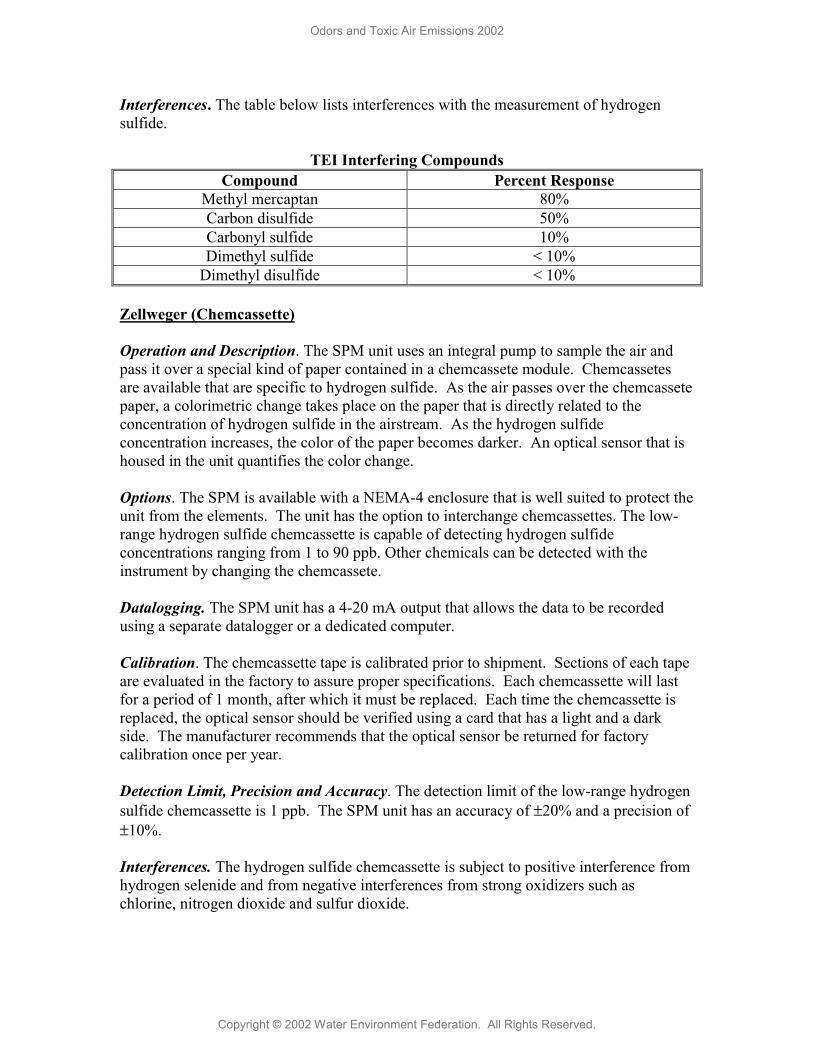
Interferences. The table below lists interferences with the measurement of hydrogen sulfide.

TEI Interfering Compounds Compound Percent Response

Methyl mercaptan 80% Carbon disulfide 50% Carbonyl sulfide 10% Dimethyl sulfide < 10%

Dimethyl disulfide < 10% Zellweger (Chemcassette) Operation and Description. The SPM unit uses an integral pump to sample the air and pass it over a special kind of paper contained in a chemcassete module. Chemcassetes are available that are specific to hydrogen sulfide. As the air passes over the chemcassete paper, a colorimetric change takes place on the paper that is directly related to the concentration of hydrogen sulfide in the airstream. As the hydrogen sulfide concentration increases, the color of the paper becomes darker. An optical sensor that is housed in the unit quantifies the color change. Options. The SPM is available with a NEMA-4 enclosure that is well suited to protect the unit from the elements. The unit has the option to interchange chemcassettes. The low-range hydrogen sulfide chemcassette is capable of detecting hydrogen sulfide concentrations ranging from 1 to 90 ppb. Other chemicals can be detected with the instrument by changing the chemcassete. Datalogging. The SPM unit has a 4-20 mA output that allows the data to be recorded using a separate datalogger or a dedicated computer. Calibration. The chemcassette tape is calibrated prior to shipment. Sections of each tape are evaluated in the factory to assure proper specifications. Each chemcassette will last for a period of 1 month, after which it must be replaced. Each time the chemcassette is replaced, the optical sensor should be verified using a card that has a light and a dark side. The manufacturer recommends that the optical sensor be returned for factory calibration once per year. Detection Limit, Precision and Accuracy. The detection limit of the low-range hydrogen sulfide chemcassette is 1 ppb. The SPM unit has an accuracy of ±20% and a precision of ±10%. Interferences. The hydrogen sulfide chemcassette is subject to positive interference from hydrogen selenide and from negative interferences from strong oxidizers such as chlorine, nitrogen dioxide and sulfur dioxide.



Draeger-Tubes Draeger-Tubes may be employed in passive sampling applications using diffusion Draeger-Tubes or in active sampling applications using a Draeger-Tube measurement system consisting of a Draeger-Tube and a Draeger gas detector pump. In the latter case, air is pumped through the tube which contains reagents that induce a colorimetric reaction with the contaminant being measured. In most cases, the contaminant concentration is a function of the length of the stain in the tube. In some instances, the contaminant concentration is a function of the intensity of the stain. In this case, the tube is compared to a reference to estimate the concentration. The Draeger-Tube measurement system can be used for short-term measurement (10 seconds to 15 minutes) or long-term measurements (up to 8 hours). Diffusion Draeger-Tubes require sampling times ranging from 1 to 8 hours. There are over 200 Draeger-Tubes available for measurement of over 350 gases and vapors. There are several different types of hydrogen sulfide Draeger-Tubes that employ three different chemistries as follows:

1) H2S + Pb2+ → PbS + 2H+ 2) H2S + HgCl2 → HgS + 2HCl 3) H2S + Hg2+ → HgS + 2H+

Interferences for reaction 2 include mercaptans and nitrogen dioxide. The standard ranges for these Draeger tubes range from 0.2 ppm to 40% volume hydrogen sulfide. Their accuracy ranges from ± 5 to 20 percent. Optical Remote Sensing Operation and Description. Another analytical technique that can be used to measure hydrogen sulfide is remote optical sensing using open-path spectroscopy. In this method, a beam of infrared (IR) or ultraviolet (UV) light is propagated along a given pathlength (up to 1 kilometer but the average is 100 meters). (Minnich, et.al) The light is either reflected by a retroreflector back to a detector or the light source and detector are at opposite ends of the pathlength. As the light passes through the contaminant plume, hydrogen sulfide absorbs light of a certain wavelength, and the quantity absorbed is measured and correlated to a concentration. Detection limits are <1 ppm over path lengths of several hundred meters. Several readings are taken along a contaminant plume to establish a concentration profile and determine the location of maximum contaminant concentration. Minimum Pathlength and Detection Limit. The minimum pathlength required can be calculated by taking a contaminant’s detection limit reported in ppm-meters (ppm-m) and dividing it by the contaminant’s average concentration in the plume. For example, the detection limit of hydrogen sulfide is 5 ppm-m; if its average concentration were 50 ppb, then a pathlength of 100 meters would be required.



Interferences. Traditional systems such as the Fourier-transform infrared (FTIR) system are subject to interference from compounds that have similar absorption characteristics to hydrogen sulfide. However, there are commercially available laser systems that can emit light beams within a narrower wavelength range and therefore avoid interferences. Currently, there is a portable laser device (11 pounds) commercially available called GasFinder made by Boreal Laser Inc. (Thornton, et.al) Examples of applications include monitoring hydrogen sulfide emissions from a refinery and detecting sources of hydrogen sulfide leaks in sulfur plants. The application of this technology is limited in odor studies because of the pathlengths required. LIQUID PHASE CHARACTERIZATION In odor surveys, where wastewater is the source of odorous emissions, the wastewater is also characterized to obtain a broader picture of the odor potential of the wastewater and to confirm measurements of hydrogen sulfide in the air phase. Wastewater characterization consists of the following tests: Dissolved Sulfide. Total, and as needed dissolved sulfide, is measured onsite using the methylene blue method. The analyses are conducted using a field test kit known as a LaMotte kit. This test method has been found to yield highly reproducible results. pH. The pH of the water is measured because of the impact pH has on the distribution of sulfide species. As the pH is lowered the equilibrium shifts so that the fraction of hydrogen sulfide increases and the fraction of hydrosulfide decreases. Hydrogen sulfide is the volatile species and is the source of many odors. Hydrosulfide is soluble in water and does not enter the gas phase. Oxidation-Reduction Potential (ORP). ORP measures the oxidative state of a water. The more reduced a water the greater the tendency that sulfur-containing compounds will be present as sulfide. ORP is measured with a probe similar to a pH probe. Temperature. The vapor pressure of volatile compounds increases with temperature. Measured temperature provides a relative indication of the volatility of compounds. CONCLUSIONS • Many of the compounds responsible for odor emissions at wastewater plants have

been identified and their odor threshold and recognition concentrations determined. • There are numerous methods used to estimate odor emissions from wastewater. The

use of the emission isolation flux chamber is the most commonly used method. This is because it has been shown to be cost-effective, and the measurements obtained using the flux chamber are independent of meteorological conditions.



• There are three general approaches to collecting air samples as part of estimating odor

emissions: whole air sampling; passing the air that is to be sampled through a sorbent; and bubbling the air that is to be sampled through a solution in a midget impinger.

• Sensory analysis and odor measurement protocols are well developed in the U.S. and

internationally. Acceptance of international sensory analysis and odor measurement protocols is pending.

• The reduced sulfur scan using a chemiluminesence detector, which measures for 20

compounds, is a commonly used tool to identify odorous reduced sulfur compounds. • There are numerous portable and handheld hydrogen sulfide and total reduced sulfur

instruments that are available. The Jerome meter is one of the more commonly used and reliable hand-held field instruments used to measure hydrogen sulfide. This device also measures for other reduced sulfur compounds when they are present. Other devices include the Interscan, the Thermo Environmental Instruments Model 45C and the Zellweger (chemcassette).

• Estimating odor emissions from wastewater includes measuring the wastewater for

the parameters: dissolved sulfide, pH, ORP and temperature. REFERENCES American Industrial Hygiene Association (AIHA). “Odor Thresholds for Chemicals with Established Occupational Health Standards”. 1989 ASTM E544-99: Standard Practice for Suprathreshold Intensity Measurement, American Society for Testing and Materials, Philadelphia, PA. 1989 ASTM D 1945–96; Standard Test Method for Analysis of Natural Gas by Gas Chromatography ASTM E679-91: Standard Practice for Determination of Odor and Taste Thresholds By a Forced-Choice Ascending Concentration Series Method of Limits, American Society for Testing and Materials, Philadelphia, PA. 1991. Dravineks, A., Jarke, F. “Odor Threshold Measurement by Dynamic Olfactometry: Significant Operational Variables”, Journal of the Air Pollution Control Association. Vol. 30, No. 12. December 1980. Keith, L. H. (ed), "Environmental Sampling and Analysis: A practical guide", Lewis Publishers, Michigan, 1991.



McGinley, Charles M., Mahin, Thomas D., Pope, Richard J. “Elements of Successful Odor/Odour Laws”, WEF Odor/VOC 2000 Specialty Conference. April 2000. McGinley, Charles M., McGinley, Michael A., McGinley, Donna L. “‘Odor Basics’, Understanding and Using Odor Testing” The 22nd Annual Hawaii Water Environment Association Conference, Honolulu, Hawaii. June 6-7, 2000. M. McGinley, C. McGinley, The New European Olfactory Standard: Implementation, Experience and Perspectives, AWMA Conference, 2001. Minnich, T.R., Scotto, R.L., Leo, M.R., “Sampling and Analysis of Airborne Pollutants: Remote Sensing of Volatile Organic Compounds (VOCs): A Methodology for Evaluating Air Quality Impacts During Remediation of Hazardous Waste Sites”, pgs. 274-255, 1993 Morton, C. M., Federici, N. J. Odor Control Pilot Plant Testing and System Design for a Fermentation Plant, WEF Control of Odors and VOC Emissions Conf., Houston, TX, 1997 National Academy of Sciences (NAS). Odors from Stationary and Mobile Sources. Washington, D.C. 1979. OSHA Analytical Methods Manual, 2nd Edition, Part 2, Inorganic Substances, “Ammonia in Workplace Atmospheres – Solid Sorbents” Method ID 188. 1991 Perry and Chilton Chemical Engineering Handbook. 5th Ed. McGraw-Hill, 1973. Ruth, J. H., Odor Thresholds and Irritation Levels of Several Chemical Substances: A Review, Am. Ind. Hyg. Assoc. J, March 1986 Thornton, E., Bowmar, N., “The Application of a Laser-Based Open-Path Spectrometer for the Measurement of Fugitive Emissions and Process Control”, A&WM Association Conference, Raleigh, North Carolina, October 28th, 1999 USEPA, Eklund, Bart, C. Schmidt. Air/Superfund National Technical Guidance Series – Vol. II – Estimation of Baseline Air Emissions at Superfund Sites. August 1990. USEPA, “Measurement of Gaseous Emission Rates From Land Surfaces Using an Emission Isolation Flux Chamber – User’s Guide,” EPA 600/8-86/008 (NTIS PB86-223161), February 1986. Water Environment Federation. (WEF) Manual of Practice No. 22. American Society of Civil Engineers. (ASCE) Manuals and Reports on Eng. Practice No. 82. Odor Control in Wastewater Treatment Plants. 1995



methods for estimating odor emissions scott...

Documents