methods of functional analysis in elasticity · 2012-12-26 · chapter methods of functional...
TRANSCRIPT
CHAPTER
METHODS OF FUNCTIONAL ANALYSIS IN ELASTICITY
The purpose of this chapter is to present some basic theorems in elasticity concerning the boundary value problems of elastostatics and elastodynamics. The techniques are primarily those of linear and nonlinear functional analysis. The first five sections are motivated by questions of existence and uniqueness, but the results turn out to bear on basic questions such as: what constitutive inequalities should one impose? Section 6.6discusses what is currently known (to the authors) concerning a longstanding problem: are minima of the energy stable? This turns out to be a very subtle yet significant point. The final section gives an application of nonlinear analysis to a control problem for a beam as a sample of how the general machinery can be used in a problem arising from nonlinear elasticity.
This chapter is not intended to be comprehensive. Some of the important topics omitted are the methods of variational inequalities (see Duvaut and Lions [1972]) and, except for a few illustrative examples, the existence theory for rods, plates, and shells. The topics omitted include both the approximate models such as the von Karmen equations and the full nonlinear models (see, for example, Ciarlet [1983], Berger [1977], Antman [1978a], [1979b], [1980c], and references therein).
6.1 ELLIPTIC OPERATORS AND LINEAR ELASTOSTATICS
This section discusses existence and uniqueness for linear elastostatics. The methods used are based on elliptic theory. Basic results in this subject are stated without proof; for these proofs, the reader should consult, for example, Agmon

316 METHODS OF FUNCTIONAL ANALYSIS IN ELASTICITY CH. 6
[1965], Friedman [1969], Morrey [1966], or Wells [1980]. These results are then applied to linear elastostatics. The methods and emphasis here differ slightly trom those in the important reference work of Fichera [I972a].
To simplify notation and the spaces involved, we shall explicitly assume the body <B is a bounded open set n in IR" with piecewise smooth boundary. The reader is forewarned that standard usage and a number of notational conflicts have resulted in us adopting various notations for the volume element throughout this chapter.
The linearized equations under consideration are as follows (see Chapter 4):
div(a· Vu)(x) = /(x), x E n, (1)
where / = -ph - div (J, h is the body force, (J is the Cauchy stress in the configuration we are linearizing about, and a = (J Q9 3 + c is the corresponding elasticity tensor; we assume a is Coo. We assume boundary conditions of displacement or traction are used and shall assume them to be homogeneous. [This is no real loss of generality, for if the boundary conditions are not homogeneous, say u equals some displacement iI on an, replace / by / + div(a· Vii) andubyu-il.]
1.1 Definitions Let V denote the Hilbert space of all displacements u: n -+ IR" that are square integrable:
II u IIi. = In IluW dv < 00.
Let HI denote the Hilbert space of all displacements u: n -+ IR" that belong to V and such that the gradient Vu (initially only a distribution) is also an V tensor. The HI-norm is defined by
IlullHI = (InlluWdv + In IIVull2 dvY/2.
Similarly, define HS for positive integers s, with the convention HO = V. (One can show that HI is a Hilbert space: basic facts about these Sobolev spaces will be given shortly without proof; we shall not require these detailed proofs, which are contained in the references cited earlier and Adams [1975]. See Box 1.1 for further information and some sample proofs.)
If p is a real number (1 < p < 00), LP denotes the space of displacements u such that
II U ilL' = (In II u W dv rIP < 00
(with II u IILoo = ess SUPxen II u(x) ID. Define WI,p to be the space of u E U such that Vu is U as well, with norm
II u IIwI,' = (II u IIf. + II Vu IIf.)IIP. Similarly, define the Sobolev spaces Ws'P for s a positive integer. I In this
IFor s not an integer, these may still be defined by means of the Fourier transform; see Box 1.1.
CH. 6 METHODS OF FUNCTIONAL ANALYSIS IN ELASTICITY 317
notation, we have the following coincidences:
Ws •Z = HS.
Let Hi denote the set of u E HZ with homogeneous boundary conditions of displacement or traction (or both) imposed; that is,
u = 0 on ad and (a.Vu).n = 0 on a. (where one of ad or a. may be empty). (One has to show that Hi is a welldefined closed subspace of HZ; this is true and relies on the so-called "trace theorems"; cf. Adams [1975], Section 5.22 and p. 330 below.)
Define the linear operator
A: Hi -> £2 by A(u) = div(a·Vu). (2)
Problem (1) can be phrased as follows: given f E £2, can we solve Au = f? Throughout this section, we shall make the following:
1.2 Assumptions (i) The elasticity tensor a is hyperelastic; that is,
(ii) The elasticity tensor a is strongly elliptic; that is, there is an f > 0 such that
aabCd(X)~i;crtbrtd > f II ~ W 1111 W for all vectors ~,11 E lRn and all x E Q.
1.3 Proposition Assumption (i) is equivalent to symmetry of A; that is,
<Au, v> = <u, Av> for u, v E Hi, where ( , ) is the £2 inner product.
Proof Assume (i). Then
(Au, v) = fa (aabcdUcld)lbVa dv.
We can integrate by parts noting that the boundary terms are zero, giving the following:
(Au, v) = - fa aabcducldValb dv.
(This requires some further justification since u and v are not smooth; this is done by an approximation argument which is omitted.) This expression is symmetric in u and v. The converse is left as an exercise. I
1.4 Definition The mapping B from HI X HI to lR defined by
(3)
(which is a continuous symmetric bilinear form) is called the Dirichlet form.

318 METHODS OF FUNCTIONAL ANALYSIS IN ELASTICITY CH. 6
The next proposition, discussed in Box 1.1, relates the Dirichlet form and strong ellipticity.
1.5 Proposition Let A be defined as above, and let (i) of 1.2 hold. Then strong ellipticity is equivalent to Garding's inequality:
{
There are constants c > 0 and d > 0 such that
B(a, a) > cllallJr, - dll a IIi, for all a E HI.
Problem 1.1 Use Garding's inequality and the inequality 2ab < Eaz + (I/E)b 2 to show that -(Au, u) > clliallJr, - dliialli, for all a E Hi, for suitable positive constants C I and d l •
There are some technical difficulties with the mixed problem that will force us to make hypotheses on ad and a~ that are stronger than one would ideally like. Specifically, for the validity of certain theorems, we shall need to assume that the closures of ad and a~ do not intersect. This means, in effect, that ad and iJ. do not touch. An example of something that is allowed by this is when <B is an annulus, with ad the outer boundary and a. the inner boundary. For the pure displacement or traction problem, we likewise require a<B to be smooth, say CI. Again this is an unpleasant assumption', for it eliminates bodies with corners.
The assumptions in the previous paragraph may well be just technical and not necessary, but to eliminate them would require nontrivial modifications of what follows. The difficulty lies with the regularity of solutions; for example, if one is solving tJ.ifJ = f with Dirichlet boundary conditions and a<B has corners, the issue of whether or not ifJ is in HZ whenf is in J.2 is delicate. If <B is a square or a cube, this is true and can be seen by using Fourier series. If the angles are not 90°, however, this assertion need not be true in Sobolev spaces, but analogous results may be true in other spaces. As far as we know, this theory has not yet been developed, except for isolated cases. (See also the remarks on p. 371.)
For both the linear and nonlinear theories, these problems do not really affect the existence question if one seeks a generalized solution with less regularity. However, if regularity is desired, or if the inverse function theorem is to be used, the above assumptions must be made, or else the spaces must be modified. The situation calls for further research to see if these difficulties are just technical or are of physical interest. Presumably the modifications in the spaces needed correspond to known asymptotic solutions near corners, cracks, etc.
For the rest of this section we shall make the assumptions of 1.2 and those on a<B above without explicit mention.
1.6 Basic Facts about Elliptic Operators
(i) Elliptic estimates. If u E H;, then for each s > 2 there is a constant K such that

CH. 6 METHODS OF FUNCTIONAL ANALYSIS IN ELASTICITY 319
More generally, jf 1 < p < 00,
II ullw',p < K(II Aullw'-"p + II u lip)·
The proof is omitted. See Box 1.1 for the proof in a simple case. (ij) The kernel of A is finite dimensional. [Proof' The elliptic estimates
show that II u IIH' < C II u IlL' on Ker A. Rellich's theorem, which states that the inclusion HS -> Hr (s > r) is compact, then implies that the unit ball in Ker A is compact. Hence it is finite dimensional. 2] We also get II u IIH' < Cli U IlL' so Hoo = n.;;o:o HS c Ker A. Since Hs c Ck if s > nl2 + k (see Box 1.1), HOO = Coo, so elements of Ker A are smooth in this case. Similarly, the spectrum of A is discrete and each eigenvalue has finite multiplicity.
(iii) The range of A is closed in L2. The outline of the proof of this for those knowing some functional analysis requires the following facts:
(1) Let T be a closed linear operator in a Banach space X with domain 5)(T) (T closed means its graph is closed). Then if T is continuous, 5)(T) is closed.
This follows from the definition.
(2) Let ~ and cy be Banach spaces, C: X ---> cy a 1 - 1 continuous linear map with closed range, and B: X -> cy a compact linear operator. Suppose C + B is 1 - 1. Then C + B has closed range.
Proof The operator (C + B)-I defined on Range(C + B) is closed since the inverse of a 1 - 1 closed operator is closed (consider the graphs). Thus, by (1), it suffices to show that (C + B)-I is continuous. Suppose that (C + B)-IYn = Xn and Yn -> O. Suppose Xn + O. By passing to a subsequence, we can suppose II Xn II > f > O. Let xn = xnlll Xn II. Then
II(C + B)(xn) II = II;nllll(C + B)xnll = ::~::: < ; IIYnll,
so (C + B)(xn) -> O. Since B is compact and II xn II = 1, we can suppose B(xn) converges. Thus C(xn) converges too. Since C has closed range, C(xn) -> Cx for some X E X. By the closed graph theorem, C has a bounded inverse on its range. Thus xn -> X, so II x II = 1. But (C + B)(xn) -> 0 and so (C + B)(x) = 0 and thus x = 0, a contradiction.
(3) Now, let X = Hi, 'Y = L2 X L2, Cu = (Au, u), and Bu = (0, -u). Let X be the Hilbert space orthogonal complement of ker (C + B) in fr, and restrict C and B to X. By construction, C + B is 1 - 1. Clearly Cis 1 - 1; moreover, using the sum norm on cy,
II Cull'Y = II Au I!£. + IluliL' > ~llull!l: by the elliptic estimate (i) with ~ = II K. This estimate shows directly that the
2 A Banach space is finite dimensional if and only if its unit ball is compact (another theorem of RelIich).

320 METHODS OF FUNCTIONAL ANALYSIS IN ELASTICITY CH. 6
range of C is closed. Finally, B is compact by Rellich's theorem. Thus, by (2), (C + B)(u) = (Au, 0) has closed range. Hence A has closed range. I
(iv) Weak solutions are strong solutions. Suppose u E L2,/ E L2, and <u, Av) = </, v) for all v E H;. Then u E H; and Au = /
Proof We sketch the proof of (iv) as follows: This is a regularity result. The statement <u, Av) = </, v) implies that Au = / in the sense of distributions, so Au E U. Thus, as in the basic elliptic estimate (i), u E H2. In fact, the most delicate part here is that u is H2 near the boundary, a relatively deep fact. That u must satisfy the boundary conditions comes about formally as follows. Integrating by parts,
<u, Av) = t u.div(a. Vv) dv
= - r Vu.a.Vv dv + f u.[a·Vv·nJ da Jg ag
= r div(a. Vu)v dv + f {u·[a· Vv·nJ - v·[a. Vu.n]} da, Jg ag
Suppose the boundary conditions are v = 0 on an. If this is to equal </, v) for all v E H:, then first take v of compact support in n to get div(a. Vu) =/ Thus, we are left with the identity
f u·[a.Vv·nJ da = O. ag
Since no condition is imposed on a.(Vv·n] on an, u must vanish on an. A similar argument holds for the traction or mixed case. I
From these facts we can deduce the following crucial result for symmetric elliptic operators;
1.7 Fredholm Alternative Theorem U = Range A EEl Ker A, an L2 orthogonal sum.
Proof By 1.6(iii), Range A is closed. Let ~ be its U orthogonal complement. We claim that ~ = Ker A. This will prove the result. First of all, if u E Ker A and/= Av E Range A, then as A is symmetric, <u,/) = <u, Av) = <Au, v) = O. Conversely, if u E ~, then <u, Av) = 0 for all v E H;. Thus by 1.6(iv) u E H: and Au = 0; that is, u E Ker A. I
Remarks From the elliptic estimates, the decomposition in 1.7 has a regularity property;
Ws,p = Range(A I H: n Ws+2,P) EEl Ker A.
For non-symmetric elliptic operators, the Fredholm alternative reads
U = Range A EEl Ker A*,
where A* is the adjoint of A.

CH. 6 METHODS OF FUNCTIONAL ANALYSIS IN ELASTICITY 321
Problem 1.2 Use the Fredholm alternative applied to AI - A and Garding's inequality to show that AI - A: H; -> V is an isomorphism, where .A. > dl> with d1 given in Problem 1.1.
From 1.7 we obtain the following main result for our boundary value problem.
1.8 Theorem Let / E V. Then there exists a u E H; such that Au = / if and only if
<J, h) = 0 for all h E Ker A.
In this case, (i) u is unique up to addition of elements in Ker A, and (ii) if/is of class W',P, u is of class W·+ 2 ,p (up to and including the boundary).
Theorem 1.8 gives complete information on when the boundary value problem
Au =J, U E Hi is solvable for u. To be useful, one must be able to compute Ker A in a specific instance. We show how this may be done for the important case of stable classical elasticity (see Section 4.3). Thus we now deal with the case Au = div(c· Vu) on <B = n c 1R3.
1.9 Definition Let Cabcd be a classical elasticity tensor on n. We say c is uniformly pointwise stable if there is an 11 > 0 such that
E = !e·c.e > 11 II eJ12 for all symmetric e (see 3.5 and 3.6 in Section 4.3).
The argument of 3.9, Section 4.3 shows that uniform pointwise stability implies strong ellipticity, but not conversely.
1.10 Lemma If c is uniformly pointwise stable and if u E Ker A, then u is an infinitesimal Euclidean motion; i.e. a rotation or translation.
Proof If u E Ker A, then div(c. Vu) = O. Thus, multiplying by u and integrating,
0= 50 u.div(c. Vu) dv = -50 Vu·c· Vu dv.
Here we integrated by parts using the boundary conditions. By c's symmetries, Vu·c·Vu = e·c·e, where e = !£.g; that is, eab = !(Ualb + Ubla)' By 1.9 we conclude that e = 0, so u is an infinitesimal rotation or translation. I
For the displacement or mixed problem, any infinitesimal rotation must vanish since it vanishes on a portion of an containing three linearly independent points. For the traction problem any infinitesimal rotation or translation lies in Ker A. Thus, we have proved the following:

322 METHODS OF FUNCTiONAL ANALYSIS IN ELASTICITY CH. 6
1.11 Theorem For classical elasticity, a&mme c is uniformly pointwise stable, and the hypotheses on the boundary conditions preceding 1.6 hold. Then
(i) For displacement or mixed boundary conditions and any fEU, the problem div(c o Vu) =f, has a unique solution u E H~.Iff E Ws,p, then u E Ws+2,p for s > 0, 1 < p < 00,
(ii) (Traction Problem) The equation
div(c o Vu) = f, fEU
with c· Vu = 0 on an has a solution u E H~ if and only if
L/(x)o(a + bx) dv = 0,
where a is any constant vector and b is any skew-symmetric matrix. If this holds, u is unique up to the addition of a term of the form a + hx, h a skew matrix. Iff E Ws'P (s > 0, 1 < p < 00), then u E Ws+2,P.
Sometimes Korn's inequalities are used in studying results like those in Theorem 1.11; however, our presentation did not require or use them. They are very relevant for questions of stability in linear elastodynamics, as we shall see in Section 6.3. We shall state these without detailed proof (see Fichera [1972a], Friedrichs [1947], Payne and Weinberger [1961], the remark below and Box 1.1 for the proofs).
1.12 Korn's Inequalities
(i) First Inequality. For u E H~ satisfying displacement boundary conditions on ad c an, we have
Ll/e W dv > cllul/~,
for a susitable constant c > ° independent of u. (ii) Second Inequality. There is a constant c > ° such that
In 1/ e W dv + L 1/ u W dv > C 1/ u 1/;, for all u E HI.
The first inequality is fairly straightforward (see Box 1.1) while the second is more subtle. For the displacement or mixed problem, uniform pointwise stability implies that we have
-<Au, u) = In eoCoe dv > 211 I 1/ e W dv > 211C 1/ u I/~,.
So it follows that Ker A = {OJ in this case, reproducing what we found above. As indicated in 2.8, Section 5.2, this inequality will guarantee dynamic stability.
Korn's inequalities are actually special cases of Gdrdings inequality for (not necessarily square) elliptic systems. The Lie derivative operator

CH. 6 METHODS OF FUNCTIONAL ANALYSIS IN ELASTICITY 323
is in fact elliptic in the sense of systems of partial differential equations (see, for example, Berger and Ebin [1969]). Gardings inequality applied to L is exactly Korn's second inequality. The first inequality comes from the general fact that for elliptic operators with constant coefficients satisfying zero boundary conditions, Gardings inequality reads B(u, u) > ell u II~l-that is, stability. (This is seen by examining the proof; see Box 1.1.)
Box 1.1 Some Useful Inequalities
This box discusses four topics: (1) Gardings inequality (see 1.5); (2) Korn's first inequality (see 1.12); (3) a sample elliptic estimate (see 1.6(i); and (4) some key Sobolev inequalities.
(1) Garding's inequality (a) Let us prove the inequality
B(u, u) > cllull~l - dll u lIZ. in case a is strongly elliptic and is constant (independent of x). We shall also assume u is c~ with compact support in IRn.
Let fi be the Fourier transform of u:
fie;) = (2n\nI2 i. e-I~'''U(X) dx (i = ,veT).
The HI-norm of u is given by
II u 1I~1 = ~ r (a au:) 2
dx + ~ r (U I )2 dx. 1.1 JR' X I JR'
Since the Fourier transform preserves the V-norm (Plancherel's theorem), and (aul/ax})" = e/ul/i, we have
II U 1I~1 = L 1 ; 0 fie;) 12 de + L 1 fie;) 12 d;.
By strong ellipticity,
i aut auk B(u,u) = a/kl-a i-a I dx
IR' X X
= f e}el a//t1 I t1 k d; > i f I; 121 fi 12 d; JRn Rn
= f i I; 0 fi 12 d;. R'
Thus, we can take c = f and d = f. The case of variable coefficients and a general domain requires a modification of this basic idea (cf. Yosida [1971] or Morrey [1966]).
324 METHODS OF FUNCTIONAL ANALYSIS IN ELASTICITY CH. 6
(b) Relevant to Garding's inequality is the Poincare inequality, one version of which states that if u = 0 on an, then
II uiIL• < Cli DUI\L'.
In this case, HJ can be normed by II Du ilL" and so if a has constant coefficients, we can choose d = 0 in Garding's inequality.
(c) Next we discuss Hadamard's theorem [1902], which states that Gdrding's inequality implies strong ellipticity. Let us again just prove a simple case. Suppose a is constant and assume 0 E n. Choose u(x) = 1;<p(I •• x), where I; and)" are constant vectors in IRn and <p; IR ---> IR is smooth with compact support. Then
B(u, u) = fa al}klc!IA}c!kAll<p'()"·x)12 dx
= (fa I <p'().,.x) 12 dx )(al}klelc!kA}Al).
By assumption, we get
(fa I <p'().,.x) 12 dx )(aliklc!lc!kAJAl)
> c(fa I I; 12 1)" 12 <p'().,.x) dX)
+ (c - d)(fa I I; 121 <p()".x) r~ dX).
It is easy to see that we can choose a sequence of <Pn's such that
(t I <Pi).,· x) 12 dX) I t I <p~().,.x) 12 dx ---> 0 as n ---> 00.
Dividing the preceding inequality by t 1 <Pn'()".x) 12 dx and
letting n ---> 00, we see that strong ellipticity holds with f = c.
(2) Korn's first inequality Let us prove that
fie 12 dx > c II u 1 IiI.
for u a c~ displacement in IRn with compact support. As in Garding's inequality, the general case can be reduced to this one. Let Ii(l;) be the Fourier transform of u as defined above. Thus
e(l;) = 1(1; ® Ii + Ii ® ;). Therefore, by Plancherel's theorem for Fourier transforms of tensor

CH. 6 METHODS OF FUNCTIONAL ANALYSIS IN ELASTICITY 325
fields,
However,
~ (etU, + eA)2 = ~ (etu; + e;ut + 2etUie,U,) t" I"
= 4 ~ (etut) + ~ (etu; + e}UI2)
I I'¢,
+ 2(~ e1u1e,u,). I'¢,
Using the inequality 2etule,u, > -(etut + e;uJ), we get
~ (elu, + eA)2 > 2 ~ etut + ~ (etu; + e;uf) t" I I'¢,
= 2 ~ etu;. I"
Thus, Lie 12 dx > 2 III.! Du 12 dx
which gives Korn's first inequality (cf. the Poincare inequality above). As pointed out in the remark preceding this box, this inequality is,
secretly, Garding's inequality for the elliptic operator u H> e. (3) A sample elliptic estimate Suppose a is constant and strongly
elliptic and u is smooth with compact support on [Rn. We will prove the inequality
lIull~. < CCIiAulli. + II u Iii.) for a constant C. We have
lIull~· = ~ i ete;uz de + ~ f. etu; de +:E f. ut de. i,J,k Rn i,i R" t R1J
It suffices to deal with the top order terms by Garding's inequality. Now by strong ellipticity,
II Au IIi. = ~ i I ai'kle,eIUk 12 d; i,j,k,l RlI
Using ere; < teet + eJ), we get
~ i ete;uz d; < t ~ f. (c + enuz d; 4hk P 4hk r
This gives the desired inequality.

326 METHODS OF FUNCTIONAL ANALYSIS IN ELASTICITY CH. 6
(4) Some key Sobolev inequalities Let us begin by being a little more precise in our definitions of Sobolev spaces. Let n be an open set in IR" with piecewise smooth boundary. Let C~(n, 1R1) denote the maps f: n ~ IRI that have c~ extensions to maps 1. which are c~ on all of IR". If n is bounded, we set
{completion of C~(n, 1R1) in the norm,
Wk,p(n, 1R1) = . Ilfllk,p = 1: II Difli£.,
05,i:S;k
where II cf> Ii£. = (In II cf>(x) W dXr lP is the U-norm on n, D'l'is the ith
derivative of J, and we take its norm in the usual way, For p = 2 we set HS(n, 1R1) = WS,2(n, 1R1). Thus H' is a Hilbert space. (One can show that HS consists of those L2 functions whose first s derivatives, in the sense of distribution theory, lie in £2. This is called the MeyerSerrin theorem. A convenient reference for the proof is Friedman [1969].)
For general n, set C;;,(n, 1R1) = the C~ functions from n to IR" that have compact support in n. The completion of this space in the 11.lIk,p norm is denoted wt,p, and the corresponding HS space is denoted H~. For n = IR" we just write HS = H~. Again HS(IR", 1R1) consists of those L2 functions whose first s derivatives are in L2.
In order to obtain useful information concerning the Sobolev spaces Wk,p, we need to establish certain fundamental relationships between these spaces. To do this, one uses the following fundamental inequality of Sobolev, as generalized by Nirenberg and Gagliardo. We give a special case (the more general case deals with Holder norms as well as Wk,p norms).
1.13 Theorem Let 1 <q< 00, 0 <r< 00, 0 <j < m, j/m < a < 1,0 < p < 00, withj, m integers > 0; assume that
1 j ( 1 m) ( 1 -=-+a --- + l-a)-p n r n q
(1)
(if 1 < r < 00 and m - j - n/r is an integer > 0, assumej/m < a < 1). Then there is a constant C such that for any smooth u: IR" ~ IRI, we have
(2)
(If j = 0, rm < n, and q = 00, assume u ~ ° at 00 or u lies in U for some finite q > 0.)
Below we shall prove some special cases of this result. (The arguments given by Nirenberg [1959] are geometric in flavor in contrast to

CH. 6 METHODS OF FUNCTIONAL ANALYSIS IN ELASTICITY 327
the usual Fourier transform proofs and therefore are more suitable for generalization to manifolds; cf. Cantor [I 975a] and Aubin [1976].)
The above theorem remains valid for u defined on a region with piecewise smooth boundary, or more generally if the boundary satisfies a certain "cone condition."
Note: If one knows an inequality of the form (2) exists, one can infer that (I) must hold as follows: replace u(x) by u(tx) for a real t > O. Then writing ut(x) = u(tx), one has
II DiutllLP = II Diullu·ti - n/
p,
II Ut Ill." = II u Ill."· t-n(l-ol/g.
Thus if (2) is to hold for U t (with the constant independent of t), we must have j - nip = a(m - nlr) - n(1 - a)/q, which is exactly the relation (1).
The following corollary is useful in a number of applications:
1.14 Corollary With the same relations as in Theorem 1.13, for any f > 0 there is a constant K< such that
II Diu IlL" < f II Dmu IlL" + K< II U IlL" for all (smooth) functions u.
Proof This follows from 1.13 and Young's inequality: xayl-a < ax + (1 - a)y, which implies that xayl-a = (fx)O(K<y)l-o < afX + (1 - a)K,y where, K, = l/fo/(l-ol. I
Let us illustrate how Fourier transform techniques can be used to directly prove the special case of 1.14 in which n = 3, I = 1, j = 0, p = 00, m = 2, r = 2, and q = 2.
1.15 Proposition There is a constant c > 0 such that for any f > 0 andfunctionf: 1R3 -> IR smooth with compact support, we have
Ilfll~ < c(f 3/z lIfIIL' + c1/zll AfIlL')'
(It follows that if f E HZ(1R 3), then f is uniformly continuous and the
above inequality holds.)
Proof Let
j(k) = (2nl)3/z L e-1k'J'f(x) dx
denote the Fourier transform. Recall that (Aj)(k) = -II k Wj(k). From

328 METHODS OF FUNCTIONAL ANALYSIS IN ELASTICITY
Schwarz' inequality, we have
(f I J(k) I dk r < (f (f2 +d~ k W)2)(f (f2 + II k W)2IJ(k) IZ dk)
= E1.11(fZ - L\)fllz·,
f
where C I = L (1 + ~~;W)Z < 00.
CH. 6
Here we have used the fact that h ~ h is an isometry in the V-norm
(Plancherel's theorem). Thus, from f(x) = (2';)3/Z JR' elk." J(k) dk,
(2n)3/zllfll= < IIJllLl < JZf II(fZ - L\)fIIL'
< CZ(f3/2 1IfIIL' + f- I/
2 11 L\fIIL')' I
Thus we have shown that H2([R3) c CO([R3) and that the inclusion is continuous. More generally one can show by similar arguments that HS(o.) c Ck(o.) provided s > nl2 + k and ws.P(o.) c Ck(o.) if s > nip + k. This is one of the celebrated Sobolev embedding theorems.
Prohlem 1.3 Prove that the last assertion is a special case of the result in Theorem 1.13.
For 0. bounded, the inclusion Ws.P(Q) ~ Ck(o.), s > nip + k is compact; that is, the unit ball in ws.P(o.) is compact in Ck(o.). This is proved in a manner similar to the classical Arzela-Ascoli theorem, one version of which states that the inclusion CI(o.) c CO(o.) is compact (see Marsden [1974a], for instance). Also, ws.p(o.) c Ws'.P'(o.) is compact if s > s' and p = p' or if s = s' and p > p'. (See Friedman [1969] for the proofs.)
We already saw one application of Rellich's theorem in our proof of the Fredholm alternative. It is often used this way in existence theorems, using compactness to extract convergent sequences.
As we shall see later, compactness comes into existence theory in another crucial way when one seeks weak solutions. This is through the fact that the unit ball in a Banach space is weakly compact-that is, compact in the weak topology. See, for example, Yosida [1971] for the proof (and for refinements, involving weak sequential compactness).
We shall give another illustration of Theorem 1.13 through a special case that is useful in the study of nonlinear wave equations. This is the following important inequality in [R3:
II u ilL" < Cli Du IlL"

CH. 6 METHODS OF FUNCTIONAL ANALYSIS IN ELASTICITY 329
1.16 Proposition Let u: 1R3 -+ IR be smooth and have compact support. Then
soC=~.
Proof 3 From
one gets
s~pl u3(x, y, z) I <3 L~ IU2 ~i I dx.
Set I = f u6 dx and write JsP
1= t: (Sf I u3" u31 dy dZ) dx
< r~[(s~p r~lu3Idz)(r~ s~plu3IdY)Jdx
< 9 L~ [(ff IU2 ~I dy dz)(ff IU2 ~~I dy dZ) ] dx·
Using Schwarz' inequality on this gives
~ ~
I <9 L~ [(Sf u4 dy dZ) (ff (~;r dy dz yl2 (ff (~~r dy dz r/] dx -~ -~
~ ~ ~
< 9 m~x (ff u4 dy dZ) (fff (~;) 2 dx dy dZ) 1/2 (fff (~~) 2 dx dy dZ) 1/2
< 36 1. I u3 ~~ I dx dy dz (1. (~;) 2) 1/2 (1. (~~) 2) 1/2
< 36~T (1. (~irr/2 (1. (~;rr/2 (1, (~~rr/2. Now using the arithmetic geometric mean inequality ra;;jb rc < (a ~ b ~ c)/3 gives
I < 36~TU~, II grad u 112)3/2/33/2.
3Following Ladyzhenskaya [1969].

330 METHODS OF FUNCTIONAL ANALYSIS IN ELASTICITY CH. 6
That is,
One can use the same technique to prove similar inequalities. There is another important corollary of Theorem 1.13 that we shall
prove~ The techniques can be used to determine to which Ws,p space a product belongs.
1.17 Corollary For s> n12, Hs(lRn) is a Banach algebra (under
pointwise multiplication). That is, there is a co'tstant K> 0 sflch that for u, v E HS(lRn
),
Ilu·vIIH• < KII~IIH.llvIIH" This is an important property of Hs not satisfied for low s. It certainly
is not true that L2 forms an algebra under multiplication.
Proof Choose a = j/s, r = 2, q = 00, p = 2s/j, m = s (0 <j < s) to obtain
II Dju IIL"I! < const.11 DSu IIr.s II u II';'-J/' < const.11 u IIH" (See 1.15.) Letj + k = s. From Holder's inequality we have
II DJu·Dkv Iii. < II Dju Iii,·!! II Dkv liz"" < const.11 u II~·II v II~··
Now DS(uv) consists of terms like Dju· DkV , so we obtain
II D'uv IlL' < const.1I u liB' II V IIH" Similarly for the lower-order terms. Summing gives the result. I
The trace theorems have already been mentioned in 1.1. Generally, they state that the restriction map from Q to a submanifold mz c Q of codimension m induces a bounded operator from W"p(n) to Ws-(l/mp),p(mz). Adams [1975] and Morrey [1966] are good references; the latter contains some useful refinements of this.
There are also some basic extension theorems that are right inverses of restriction maps. Thus, for example, the Calderon extension theorem asserts that there is an extension map T: WS,P(Q) ---> WS,P(lRn
) that is a bounded operator and "restriction to Q" oT = Identity. This is related to a classical Ck theorem due to Whitney. See, for example, Abraham and Robbin [1967J, Stein [1970J, and Marsden [1973a].
Finally, we mention that all these IRn results carry over to manifolds in a straightforward way. See, for example, Palais [1965] and Cantor [1979J.
Problem 1.4 Prove a Ws, P version of the ro-lemma given in Box 1.1, Chapter 4, by using the results of this box.

CH. 6 METHODS OF FUNCTIONAL ANALYSIS IN ELASTICITY 331
Box 1.2 Summary of Important Formulas for Section 6.1
Sobolev Spaces on n c [Rn
£2 = {u: n ---> [Rn I In II u2 11 dv < oo} <u, v) = fo U·V dv = fo ua(x)va(x) dx
HS = {u: n ---> [Rn lu, Du, ... , DSu are in L2} norm: Ilull~' = Ilulli, + ... + II Dsulli,. H; = {u E H21 u satisfies the boundary conditions (displacement,
traction or mixed)} Ws,p = {u: n ---> [Rn I u, Du, ... , DSu E LP}
Symmetric Elliptic Operator Form: Au = div(a·Vu) (Au)a = (aabCducld)lb Symmetry: aabcd = acdab, <Au, v) = <u, Av) for u, v E H; Strong ellipticity: aabcdeaec'1b'1d > f II ~ 1121111112 for some f > 0
and all ~, 11 E [Rn
Gdrding's Inequality (<:> Strong Ellipticity) B(u, u) > cllull~l - dllulli, for all u E HI, where
B(u,v)= fo Vu·a·Vvdv= foUa,baabcdvclddv
(= -<Au, v) for u, v E HD. Fredholm Alternative
(1) £2 = Range A E8 Ker A, an £2 orthogonal sum. (2) Au = fis solvable for u E H; if and only iff -L Ker A.
Classical Elasticity Uniform pointwise stability: 1- e·c·e > 1111 e W, 1-eabcabCdecd >
l1eabeab, implies strong ellipticity. In n c [R3, div(c· Vu) = f is solvable for u E H; using displacement or
mixed boundary conditions for any fand for traction boundary con-
ditions if fof(x)(a + bx) dx = 0 for a any constant vector and b any
3 X 3 skew matrix.
Korn's Inequalities
(1) Displacement (or mixed) boundary conditions:
In lie W dv > c II U 11~1, eab = 1-(Ualb + Ub/a)
(2) General:
In lie W dv + In II u W dv > c II U 1I~1

6.2 ABSTRACT SEMIGROUP THEORY
This section gives an account of those parts of semi group theory that are needed in the following section for applications to elastodynamics. Although the account is self contained and gives fairly complete proofs of most of the theorems, it is not exhaustive. For example, we have omitted details about the theory of analytic semigroups, since it will be treated only incidentally in subsequent sections. The standard references for semi group theory are Hille and Phillips [1957], Yosida [1971], Kato [1966], and Pazy [1974]. This theory also occurs in many books on functional analysis, such as Balakrishnan [1976].
We shall begin with the definition of a semigroup. The purpose is to capture, under the mildest possible assumptions, what we mean by solvability of a linear evolution equation
du ( dt = Au t > 0), u(O) = uo. (I)
Here A is a linear operator in a Banach space X. We are interested in when (1) has unique solutions and when these solutions vary continuously in X as the initial data varies in the X topology. When this holds, one says that Equation (I) is well-posed. If A is a bounded operator in X, solutions are given by
= (tA)k u(t) = etAuo = 2: -,-uo·
k=O k.
For partial differential equations, however, A will usually be unbounded, so the problem is to make sense out of etA. Instead of power series, the operator analogue of the calculus formula eX = limn_= (1 - x/ntn will turn out to be appropriate.
2.1 Definitions A (CO) semigroup on a Banach space X is a family {U(t) I t > OJ of bounded linear operators of X to X such that the following conditions hold:
(i) U(t + s) = U(t)oU(s) (t, s > 0) (semi group property); (ii) U(O) = Identity; and
(iii) U(t)x is t-continuous at t = 0 for each x EX; that is, limt! 0 U(t)x = x. (This pointwise convergence is also expressed by saying strong limt! 0 U(t) = 1.)
The infinitesimal generator A of U(t) is the (in general unbounded) linear operator given by
Ax = lim U(t)x - x (2) t! 0 t
on the domain~(A) defined to be the set of those x E X such that the limit (2) exists in X.
We now derive a number of properties of semigroups. (Eventually we will prove an existence and uniqueness theorem for semigroups given a generator A.)
332
CH. 6 METHODS OF FUNCTIONAL ANALYSIS IN ELASTICITY 333
For Propositions 2.2-2.12, assume that U(t) is a given Co semigroup with infinitesimal generator A.
2.2 Proposition There are constants M> 0, P > 0 such that II U(t) II < Metp for all t > O. In this case we write A E seX, M, p) and say A is the generator of a semigroup of type (M, P).
Proof We first show that II U(t) II is bounded on some neighborhood of zero. If not, there would be a sequence tn ! 0 such that II U(tn) I I > n. But U(tn)x ~ x as n ~ 00, so U(tn) is pointwise bounded as n ~ 00, and therefore by the Uniform Boundedness Theorem4 II U(tn) II is bounded, which is a contradiction.
Thus for some 0 > 0 there is a constant M such that II U(t) II < M for 0 < t < O. For t > 0 arbitrary, let n be the largest integer in t/o so t = no + -r, where 0 <-r < O. Then by the semi group property,
II U(t) II = II U(no)U(-r) II < II U(-r)1111 U(o)W < M·Mn < M·Mt/li < MetP.
where P = (I/o) log M. I
2.3 Proposition U(t) is strongly continuouss in t; that is, for each fixed x E X, U(t)x is continuous in X as a function of t E [0, 00).
Proof Let s > O. Since U(-r + s)x = U(s)U(-r)x, 2. 1 (iii) gives
lim U(t)x = lim U(-r + s)x tls dO
= U(s) lim U(-r)x = U(s)x, Tlo
so we have right continuity in tat t = s. For left continuity let 0 < -r < s, and write
II U(s - -r)x - U(s)x II = II U(s - r)(x - U(-r)x) II < Me PCS - T) II x - U(r)x II,
which tends to zero as -r ~ o. I
2.4 Proposition
(i) U(t)~(A) c ~(A);
(ii) U(t)Ax = AU(t)xfor x E ~(A); and (iii) (d/dt)U(t)xo = A(U(t)xo) for all Xo E ~(A) and t > O. In other
words,
dx ( x(t) = U(t)xo satisfies dt = Ax and x 0) = Xo.
4This theorem states that if {Ta} is a family of bounded linear operators on OC and if {TaX} is bounded for each x E OC, then the norms II Ta II are bounded. See, for example, Yosida [1971], p. 69.
SOne can show that strong continuity at t = 0 can be replaced by weak continuity at t = 0 and strong continuity in t E [0, (0) can be replaced by strong measurability in t. See Hille and Phillips [1957] for details.
334 METHODS OF FUNCTIONAL ANALYSIS IN ELASTICITY CH. (
Proof From [U(h)U(t)x - U(t)x]/h = U)t)[(U(h)x - x)/h] we get (i) and (ii) We get (iii) by using the fact that if x(t) E X has a continuous right derivative then x(t) is differentiable--.1from the right at t = 0 and two sided if t > 0. 6 I
From (i) and (ii) we see that if x E ~(An), then U(t)x E ~(An). This is often used to derive regularity results, because if A is associated with an elliptic operator, ~(An) may consist of smoother functions for larger n. Notice that we have now shown that the concept of semigroup given here and that given in 2.5, Chapter 5, agree.
2.5 Proposition ~(A) is dense in X.
Proof Let cp(t) be a COO function with compact support in [0, 00), let x E X and set
x¢ = r cp(t)U(t)x dt.
Noting that
U(s)x¢ = r cp(t)U(t + s)x dt = r cp(. - s)U(r)x d.
is differentiable in s, we find that x", E ~(A). On the other hand, given any E > 0 we claim that there is a cp (close to the "0 function") such that II x", - x II < f. Indeed, by continuity, choose 0 > 0 such that II U(t)x - x II < E if 0 < t < O. Let cp be COO with compact support in (0, 0), cp > 0 and r cp(t) dt = 1.
Then
II x", - x II = II r cp(t)(U(t)x - x) dt II < S: cp(t) II U(t)x - x II dt
< E S: cp(t)dt = E. I
The same argument in fact shows that n:=1 ~(An) is dense in X.
2.6 Proposition A is a closed operator; that is, its graph in X X X is closed.'
Proof Let Xn E ~(A) and assume that Xn -> Xo and AXn -> y. We must show that x E ~(A) and y = Ax. By 2.4,
U(t)xn = Xn + S: U(s)Axn ds.
6This follows from the corresponding real variables fact by considering /(u(t)) for / E ~*. See Yosida [1971], p. 235.
'We shall prove more than this in Proposition 2.12 below, but the techniques given here are more direct and also apply to certain nonlinear semi groups as well. See Chernoff and Marsden I1974].
CH. 6 METHODS OF FUNCTIONAL ANALYSIS IN ELASTICITY 335
Since U(s)Axn ~ U(s)y uniformly for s E [0, t], we have
U(t)x = x + s: U(s)y ds.
It follows that (dfdt+) U(t)x It-o exists and equals y. I
Next we show that integral curves are unique. (Compare 2.15, Chapter 5.)
2.7 Proposition Suppose e(t) is a differentiable curve in X such that e(t) E
:D(A) and e'(t) = A(e(t» (t > 0). Then e(t) = U(t)e(O).
Proof Fix to > 0 and define h(t) = U(to - t)e(t) for 0 < t < to. Then for-r small,
Ilh(t + -r) - h(t) II = II U(to - t - -r)e(t + -r) - U(to - t - -r)U(-r)e(t) II < MeP(to-t-T) II e(t + -r) - U(-r)e(t) II.
However,
1 1 1 -[e(t + -r) - U(-r)e(t)] = -[e(t + -r) - e(t)] - -[U(-r)e(t) - e(t)], -r -r -r
which converges to Ae(t) - Ae(t) = 0, as -r ~ O. Thus, h(t) is differentiable for 0< t < to with derivative zero. By continuity, h(to) = limtltoh(t) = e(to) = limt1to h(t) = U(to)e(O). (The last limit is justified by the fact that II U(t) II < MetP.) This is the result with t replaced by to. I
One also has uniqueness in the class of weak solutions as is explained in the optional Box 2.1.
Box 2.1 Adjoints and Weak Solutions (Balakrishnan [1976] and Ball [1977c])
Let the adjoint A*: :D(A*) c X* ~ X* be defined by :D(A*) = {v E X* I there exists aWE X* such that (w, x) = (v, Ax) for all x E :D(A)}, where ( , ) denotes the pairing between X and X*. Set A*v = w. If e(t) is a continuous curve in X and if, for every v E :D(A*), (e(t), v) is absolutely continuous and
~ (e(t), v) = (e(t), A*v) almost everywhere
that is, (e(t), v) = (e(O), v) + f: (e(s), A*v) ds, then e(t) is called a
weak solution of dxfdt = Ax.

336 METHODS OF FUNCTIONAL ANALYSIS IN ELASTICITY CH. 6
2.8 Proposition Let {U(t)} be a CO semigroup on a:. If c(t) is a weak solution, then c(t) = U(t)c(O). Conversely, for Xo E a: (not necessarily in the domain of A), then c(t) = U(t)xo is a weak solution.
Proof If Xo E :D(A), then U(t)xo is a solution in :D(A) and hence a weak solution. Since U(t) is continuous and :D(A) is dense, the same is true for Xo E a:; that is, we can pass to the limit in
<U(t)xm v) = <Xn, v) + 5: <U(-r)xm v) d-r
for Xn E :D(A), Xn ---> Xo E a:. Now suppose c(t) is a weak solution. Let wet) = c(t) - U(t)c(O). Then
w(O) = 0 and for v E :D(A*),
<wet), v) = 5: <w(-r), A*v) d-r = (5: w(-r) d-r, A*V)'
Thus, s: w(-r) d-r E :D(A) since A is closed (see 2.6). Here we have used
the fact that if A is closed, then A** c A, where we identify a: with a subspace of a:: * * . (If a:: is reflexive, A** = A; cf. Kato [1966], p. 168.) It
follows that z(t) = S: w(-r) d-r satisfies i = Az, and since z(O) = 0, z is
identically zero by 2.7. I
Ball [1977c] also shows that if the equation x = Ax admits unique weak solutions and A is densely defined and closed, then A is a generator.
We continue now to develop properties of a given semigroup of type (M, p). If P = 0, we say the semigroup is bounded, and if M = 1, we say it is quasicontractive. If M = 1 and P = 0, it is called contractive.
2.9 Proposition If U(t) is (a Co semigroup) of type (M, p) on a:, then: (i) T(t) = e-'PU(t) is a bounded semigroup with generator A - pI; (ii) there is an equivalent norm 111·111 on a: relative to which U(t) is quasi-contractive.
We shall leave the proof as an exercise. For (ii), use the norm III xiii =
sup,;;,o II e-'PU(t)x II·
2.10 Example Let a:: = V(IR) with the norm
IIJW = fl IJ(x) 12 dx + t SR\[-1,llIJ(x) 12 dx
and let (U(t)f)(x) = J(t + x). Then U(t) is a Co semi group and AJ = dfldx

CH. 6 METHODS OF FUNCTIONAL ANALYSIS IN ELASTICITY 337
with domain H!(IR) (absolutely continuous functions with derivatives in V). Here, II U(t) II < 2. If we form the norm III III, we get the usual V-norm and a contraction semigroup.
2.11 Proposition U(t) is norm continuous at t = 0 if and only if A is bounded.
Proof Choose f > 0 so that II U(t) - III < f if 0 < t < f and pick if> to be
a Coo function with compact support in [0, f) such that if> > 0 and fa' if>(t) dt = 1.
Let J¢>(x) = r if>(-r)U(-r)x d-r and note that
JiU(t)x) = r if>(-r)U(-r + t)x d-r = f if>(-r - t)U(-r)x d-r.
However,
II (Jill - I)(x) II = II r if>(-r)(U(-r)x - x) d-r II < f r if>(-r) II x II d-r = fll x II,
so II J¢> - I II < f and hence Jill is invertible. By construction
U(t)x = J;!(f if>(-r - t)U(-r)x d-r),
which is therefore differentiable in t for all x and also shows A E ffi(a:) (the set of all bounded linear operators on a:). The converse is done by noting that etA = ~:=o(tA)nl(n!) is norm continuous in t. I
Next we give a proposition that will turn out to be a complete characterization of generators.
2.12 Proposition Let A E sea:, M, P). Then:
(i) :D(A) is dense in a:; (ii) (A - A) is one-to-one and onto a: for each A > p and the resolvent
R;. = (A - At! is a bounded operator; and (iii) II (A - Atn II < MI(A - p)n for A > P and n = 1,2, ....
Note. Here and in what follows, A - A stands for AI - A, where I is the identity operator.
Proof Given x E a:, let
Then
A>P·
(U(s) - I)y;. = r e-J.tU(t + s)x dt - y;.
= eAS f.oo e-;'TU(-r)x d-r - y;.
= (e;'s - l)y;. - e;" I: e-;'tU(t)x dt.

338 METHODS OF FUNCTIONAL ANALYSIS IN ELASTICITY CH.
Hence YA E ~(A) and Ay.t = Ay.t - X. Thus (A - A) is surjective. (Taking A-00 shows that AYA -> x, which also shows ~(A) is dense, reproducing 2.5.) Thl formula
u = r e-1tU(t)(A - A)u dt, U E ~(A),
which follows from -(dldt)e-1tU(t)u = e-AtU(t)(A - A)u, shows that (A - A) i! one-to-one.
Thus we have proved the Laplace transform relation
R1x = (A - A)-IX = {O e-.ttU(t)x dt, (A> P),
from which it follows that
II(A - A)-III < fO e-).tMePt dt = AMp"
The estimate (iii) follows from the formulas
(n - I)! (A - Atnx = r e-1ttn- 1 U(t)x dt,
J~ e-pttn-I dt = (n - I)!. o J.ln
(3)
(4)
Equation (4) is proved by integration by parts and (3) follows from the relation
(~r-I (A - A)-I = (-I)n-I(n - I)! (A - Atn. I
Problem 2.1 Show that the resolvent identity Rl - Rp = (J.l - A)R1Rp holds and that J.lR1 -> Identity strongly as A -> 00.
The following Hille- Yosida theorem asserts the converse of 2.12. It is, in effect, an existence and uniqueness theorem. Uniqueness was already proved in 2.7.
2.13 Theorem Let A be a linear operator in X with domain ~(A). Assume there are positive constants M and P such that:
(i) ~(A) is dense; (ii) (A - A) is one-to-one and onto X for A > P and (A - A)-I E <B(X);
and (iii) II (A - A) II-n < MI(A - p)n (A > p, n = 1,2, ... ).
Then A E seX, M, p); that is, there exists a Co semigroup of type (M, P) whose generator is A. We shall often write etAfor the semigroup generated by A.
Proof If (A - PI) generates the semigroup U, then A generates the semigroup etPU (see 2.9). Thus it suffices to prove the theorem for P = O.
Rewrite (iii) as II (I - ~A)-n II < M (~ > 0, n = 1, ... ) by taking ~ = Ill. Thus, if x E ~(A), then (I - ~A)-IX - X = ~(I - ~A)-IAx, so (I - ~A)-I - I

CH. 6 METHODS OF FUNCTIONAL ANALYSIS IN ELASTICITY 339
-> 0 strongly on :D(A) as 0: ~ O. Since (I - o:A)-1 - I E <B(OC), convergence also holds on OC.
Let U,,(t) = (1 - (t/n)At", a uniformly bounded sequence of operators. We shall show it converges on a dense set. Write
it d
U,,(t)x - Um(t)x = Um(t - s)U,,(s)x I~;;~ = s-lim -d Um(t - s)U,,(s)x ds dO • S
i t ( t ) ( t )-m-l( )-"-1 = s-lim ..£ - - S A2 1 - - SAl - ..£A x ds. dO • n m m n
Thus, if x E :D(A2), we get,
IIU,,(t)x - Um(t)xll<M21IA2xllt(! + ~)t2. Thus U,,(t)x converges for x E :D(A2). But
:D(A2) = :D«(I - A)2) = Range(I - A)-2 = (l - A)-I:D(A).
Now (1 - A)-I: OC --> :D(A) is bounded and surjective. Since :D(A) c OC is dense, (1 - A)-I(:D(A» c :D(A) is dense; that is, :D(A2) c OC is dense.
Let U(t)x = s-lim,,_oo U,,(t)x. Clearly, II U(t) II < M, U(O)x = x, and U(t + s) = U(t)oU(s). Since U,,(t)x -> U(t)x uniformly on compact t-intervals for x E
:D(A2) and this is dense, U(t)x is t-continuous. Thus we have a Co semigroup. Let A' be the generator of U(t). We need to show that A' = A. For x E :D(A),
d (t )-1 dt U,,(t)x = A 1 - nA U,,(t)x.
Thus
U,,(t)x = x + s: (I - ~ Ar 1
U,,(s)Ax ds,
and so
U(t)x = x + s: U(s)Ax ds.
Therefore x E :D(A') and A' ::J A. But (I - A')-1 E <B(OC) by the previous proposition and (1 - A)-1 E <B(OC) by assumption, so they must agree. I
We shall give some concrete examples of how to check these hypotheses below and in the next section. In this regard, note that if M = 1, we -have a quasi-contractive semigroup and verification of (iii) for n = 1 is sufficient. Also, as the proof shows, it suffices to verify (ii) and (iii) for some sufficiently large 1. Finally, we note that if (ii) and (iii) hold for Ill> p, then U(t) is a group-that is, is defined for all t E IR, not just t > O.
For applications, there are two special verisions of the Hille-Yosida theorem that are frequently used. These involve the notion of the closure of an operator. Namely, A is called closable if the closure of the graph of A in OC x OC is the graph of an operator; this operator is called the closure of A and is denoted A. In practice, this often enlarges the domain of A. (For example, the Laplacian

340 METHODS OF FUNCTIONAL ANALYSIS IN ELASTICITY CH. 6
V2 in ~ = L2 may originally be defined on smooth functions satisfying desired boundary conditions; its closure will extend the domain to Hi.)
2.14 First Corollary A linear operator A has a closure A that is the generator of a quasi-contractive semigroup on ~ if and only if (i) ~(A) is dense and (ii) for 1 sufficiently large, (1 - A) has dense range and 11(1 - A)x II > (1 - ft) II x II.
Proof Necessity follows Proposition 2.12. For sufficiency, we use the following:
2.15 Lemma (a) Let B be a closable linear operator with a densely defined bounded inverse B-1. Then (B-1) is injective, and (B)-I = (B-1).
(b) Suppose that A is a densely defined linear operator such that (1 - A)-I exists, is densely defined, with 11(1 - A)-I II < Kl1for large 1. Then A is closable. (Hence, by part (a), (1 - A) is invertible, with (1 - A)-I = (1 - A) I.)
Proof (a) Since B-1 is bounded, B-1 is a bounded, everywhere-defined operator. Suppose that B-Iy = O. We will show that y = O. Let Yn E Range of Band Yn -> y. Then Yn = BXn for Xn E ~(B), and Ilxnll < IIB-IIIIIYnll- O. Since B is closable, we must have Y = O. Thus fFT is injective and (a) follows.
(b) We shall first show that 1R;. ---> I as 1----> 00, where R;. = (1 - A)-I by definition. By assumption, II R;.II < KIA. Now pick any x E ~(A). Then x = R;.(A - A)x, so x = AR;.x - R;.Ax, and II R;.Ax II «KIA) II Ax 11---> 0 as A----> 00.
Thus 1R;. -> I strongly on ~(A). But ~(A) is dense and liAR;. II < K for all large A, so AR;. --> Ion the whole of~.
To prove that A is closable, we suppose Xn E ~(A), Xn ---> 0, and AXn ----> y. We claim that y = O. Indeed, choose a sequence An ---> 00 with AnXn -> O. Then (An - A)xn + Y ----> O. Since II AnR;'n II < K, we have AnR;.J(An - A)xn + y] --> O. Thus, AnXn + AnR;'nY ---> O. But AnXn ---> 0 and AnR;'nY ---+ y, so Y = o. I
The rest of 2.14 now follows. Indeed, A satisfies the conditions of part (b) of the lemma, and hence A satisfies the hypothesis of the Hille-Y osida theorem with M = 1). I
Now we give a result in Hilbert space. We will sometimes refer to this result as the Lumer-Phillips Theorem. 8 For applications we shall give in the next section, it will be one of the most useful results of this section.
2.16 Second Corollary Let A be a linear operator in a Hilbert space X. Then A has a closure A that is the generator of a quasi-contractive semigroup on X (that is, A E S(X, 1, ft)) if and onZy if:
(i) ~(A) is dense in X;
8See Lumer and Phillips [1961J for the case of Banach spaces. It proceeds in a similar way. using a duality map in place of the inner product.

CH. 6 METHODS OF FUNCTIONAL ANALYSIS IN ELASTICITY 341
(ii) <Ax, x) < p<x, x) for all x E !D(A) (If P is zero, we call A dissipative); and
(iii) (2 - A) has dense range for sufficiently large 2.
If in (iii) (2 - A) is onto, then A is closed and A E g(X, 1, P).
Proof First suppose (i), (ii), and (iii) hold. Then «2 - A)x, x) > (2 - P)· IlxW, and so by Schwarz's inequality, 11(2 - A)xll > (2 - P)l\xll. Thus A E
g(X, 1, P) by 2.15. Conversely, assume A E g(X, 1, ft). We need only show that
<Ax, x) < P<x, x) for all x E !D(A).
By 2.9 we can assume that P = 0 and U(t) is contractive. Now <x, U(t)x) < \I xliii U(t)x \I < II x Wand therefore <x, U(t)x - x) < O. Dividing by t and letting t ! 0 gives <x, Ax) < 0 as desired. I
2.17 Further Results Some additional useful results that we just quote are as follows:
1. Bounded Perturbations If A E g(X, M, P) and B E <B(X), then A + B Eg (X, M, P + II BII M) (Kato [1966], p. 495).
2. Trotter-Kato Theorem If An E g(X, M, P) (n = 1,2,3, ... ) A E g(X, M, P) and for 2 sufficiently large, (2 - An)-1 ---> (2 - A)-1 strongly, then etAn ---> etA strongly, uniform on bounded t-intervals (Kato [1966], p. 502).
Problem 2.2 Show that if !D(An) and !D(A) all have a common core 'Y c X-that is, An, A are the closures of their restrictions to 'Y, and An ---> A strongly on 'Y-then (2 - AntI ---> (2 - A)-1 strongly, from the resolvent identity (see Problem 2.1).
3. Lax Equivalence Theorem If A E g(X, M, P), and K. E <B(X) is a family of bounded operators defined for f > 0, with Ko = I, we say {K.} is:
(i) stable if II K~/n II is bounded on bounded t-intervals (n = 1,2, ... ); (ii) resolvent consistent if for 2 sufficiently large
(2 - A)-1 = s-lim (2 - .l(K. - 1»)-1 (strong limit); dO f
(iii) consistent if (d/df+ )K.(x)I.=o = Ax, x E a core of A.
The Lax equivalence theorem states that etA = s-limn~~ K'/;n uniformly on bounded I-intervals if and only if {K,} is stable and resolvent consistent (see Chorin, Hughes, McCracken, and Marsden [1978] for a proof and applications). Assuming stability, consistency implies resolvent consistency.
4. Trotter Product Formula If A, B are generators of quasi-contractive semi groups and C = A + B is a generator, then
etC = s-lim (etA/netB/n)n.
(This is a special case of 3.)

342 METHODS OF FUNCTIONAL ANALYSIS IN ELASTICITY CH. 6
5. Inhomogeneous Equations Let A E g(~, M, p) and consider the following initial value problem: Let J(t) (0 < t < T) be a continuous ~-valued function. Find x(t) (0 < t < T) with x(O) a given member of 5)(A), such that
x'(t) = Ax(t) + J(t). (I)
If we solve (I) formally by the variation of constants formula, we get
x(t) = etAx(O) + f~ e(t-.)AJ(1:) d1: (0 < t < T).
However, x(t) need not lie in ~(A); but it will ifJis a Cl function from [0, T] to ~. Then (I) is satisfied in the classical sense (Kato [1966], p. 486). For uniqueness, suppose yet) is another solution of (I), with yeO) = x(O). Let z(t) = x(t) - yet). Then z'(t) = Az(t) and z(O) = 0, so z(t) = 0 by uniqueness. Thus x(t) = yet).
6. Trend to Equilibrium Let A E g(~, 1, ft) and suppose there is a 0 > 0 such that the spectrum of eA lies inside the unit disk a positive distance 0 from the unit circle. Then for any x E ~,
etAx --> 0 as t --> +00. Indeed, if 0 < 0' < 0, we can, by way of the spectral theorem, find a new norm in which
A E g(~, 1, -0'),
from which the result follows. (See Marsden and McCracken, [1976], §2A, Slemrod [1976], and Dafermos [1968].) Abstract conditions under which spectrum eA = e"pectrum A are unfortunately rather complex (see Carr [1981] and Roh [1982]).
7. Analytic Semigroups. Ifll (' - A)-l II < MIl' I for' complex and belonging to a sector I arg' I < nl2 + (j) «(j) > 0), then A generates a bounded semigroup Vet) that can be extended to complex t's as an analytic function of t (t =1= 0). For real t > 0, X E ~ one has V(t)x E 5)(A) and
II dn~~)x II < (const.)·11 x II·rn•
Consult one of the standard references for details.
2.18 Comments on Operators in Hilbert Space and Semigroups The results here are classical ones due to Stone and von Neumann, which may be found in several of the aforementioned references. A densely defined operator in Hilbert space is called symmetric if A c A*; that is, <Ax, y) = <x, Ay) for all x,y E
5)(A) (see Box 2.1 for the definition of A*; replace ~* by ~ in Hilbert space), self-adjoint if A = A* (i.e., A is symmetric and A and A* have the the same domain), and essentially selj:adjoint if A is self-adjoint.
For the first two results following, ~ is assumed to be a complex Hilbert space.
1. Let A be closed and symmetric. Then A is self-adjoint if and only if A + )J
is surjective when 1m A. =1= O.
CH.6 METHODS OF FUNCTIONAL ANALYSIS IN ELASTICITY 343
Problem 2.3 (a) Show that a symmetric operator is closable. (b) By consulting a book on functional analysis, prove 1.
2. (Stone's Theorem) A is self-adjoint if and only if iA generates a oneparameter unitary group.
Proof From the symmetry of A and II (A + A)X W > 0, we get II(A + A)X II > 11m A III x II, and so for 2 real, 11(2 - iA)x II > 12 III x II. Thus 2 results from 1 and the Hille-Y osida theorem. I
3. (Real version of Stone's Theorem) Let A be a skew-adjoint operator on a real Hilbert space (i.e., A = -A*). Then A generates a one-parameter group of isometries and conversely. (This follows by an argument similar to 2.)
4. Let A be closed, symmetric, and A < 0; that is, <Ax, x) < 0 for all x E
!D(A). Then A is self-adjoint if and only if (2 - A) is onto (A > 0).
Problem 2.4 Use this and the Fredholm alternative to show that the symmetric elliptic operator A in Section 6.1 is self-adjoint. See Problem 1.2.
5. If A dissipative «Ax, x) < 0) and self-adjoint, then A generates a contraction semigroup. (This follows from 4 and the Lumer-Phillips theorem.)
2.19 Example (Heat Equation) Let 0 c [Rn be an open region with smooth boundary, X = V(O), Au = ilu, and !D(A) = C;;'(O), where CoCO) are the C~ functions with compact support in O. Then A generates a contraction semi group in X. (A will turn out to be the Laplacian on !D(A) = H;(O), the H2 functions with 0 boundary conditions.)
Proof Obviously A is symmetric. It follows that it is closable (Problem 2.3). Moreover, for u E !D(A),
<Au, u) = In ilu·u dx = - fa Vu·Vu dx < 0,
so A is dissipative. By the second corollary of the Hille- Y osida theorem, it suffices to show that for 2 > 0, (A - A) has dense range; that is, A is selfadjoint. Suppose v E L 2(O) is such that
«A - A)u, v) = 0 for all u E !D(A).
Then
«2 - il)u, v) = 0 for all u E C;;'CO).
By the regularity of weak solutions of elliptic equations, v is in fact C~ and v = 0 on ao. (See 1.6(iv).) Thus, setting u = v and integrating by parts,
2 In 1v l2 dx + folVvl2dx = 0,
and so v = o. I

344 METHODS OF FUNCTIONAL ANALYSIS IN ELASTICITY CH. €
The semi group produced here is actually analytic.
Problem 2.5 Show directly, using the elliptic theory in Section 6.1 (see, especially, Problem 1.2) that L\ on H; generates a semigroup. Conclude that this is A.
Problem 2.6 Generalize 2.19 to the equation du/dt = Au, where A is the operator discussed in Section 6.1.
The above example concerns the parabolic equation au/at = Au. The hyperbolic equation aZujatZ = Au is directly relevant to linear elastodynamics and will be considered in the next section.
Box 2.2 Summary of Important Formulas for Section 6.2
Semigroup in a Banach Space U(t): OC -> OC is defined for t > 0, U(t + s) = U(t)oU(s), U(O) = I,
and U(t) is strongly continuous in tat t = 0+ (and hence for all t > 0).
Infinitesimal Generator
Ax = lim U(t)x - x t~O+ t
on the domain !D(A) for which the limit exists (!D(A) is always dense). We write U(t) = etA.
Class (M, p) A E S(OC, M, P) means A is a generator of a U(t) satisfying" U(t) "
< Metfl• (Bounded if p = 0; quasi-contractive if M = 1, and con
tractive if both.)
Evolution Equation If Xo E !D(A), then x(t) = U(t)xo E !D(A), x(O) = Xo and dxJdt =
Ax. Solutions are unique if a semigroup exists.
Hille- Yosida Theorem Necessary and sufficient conditions on an operator A to satisfy A E S(OC, M, ft) are:
(i) !D(A) is dense; (ii) (A. - A)-l E ffi(OC) exists for .A. > p; and
(iii) II (A. - At"11 < MI(A. - ft)" (n = 1,2, ... ).
Useful Special Case (Lumer-Phillips Theorem) On Hilbert space X, A E S(X, 1, P) if and only if !D(A) is dense, <Ax, x) < p<x, x) for all x E !D(A), and (A. - A) has dense range. (If (A. - A) is onto, there is no need to take the closure.)

6.3 LINEAR ELASTODYNAMICS
In this section we discuss various aspects of the initial value problem in linear elastodynamics using the theory of semigroups developed in the previous section. We begin with the main result for hyperelasticity: strong ellipticity is necessary and sufficient for the equations to generate a quasi-contractive semigroup in ~ = HI X V. 9 Following this, we discuss stability and show that definiteness of the energy implies dynamical stability (the linear energy criterion). It is also shown, using a result of Weiss [1967], that if Cauchy elasticity generates stable dynamics, then it is necessarily hyperelastic. Box 3.1 describes some general abstract results for Hamiltonian systems, linear hyperelasticity being a special case. Box 3.2 shows how semigroup techniques can be used in a problem of panel flutter, and in Box 3.3 various linear dissipative mechanisms are considered, again using semigroup techniques. Finally, Box 3.4 considers symmetric hyperbolic systems and how they may be used in linear elasticity.
Table 6.3.1 shows the interrelationships between some of the topics considered in this section.
Table 6.3.1
A. Linear Hyperelasticity
Strong ellipticity
(Gcirding)
Stability (classical elasticity) it (Korn)
Elasticity tensor positive-definite
The equations of motion generate a quasi-contractive semigroup in HI x L2 (relative to some Hilbert space structure).
it Generates a contractive semigroup on
HI x £2 (relative to some Hilbert space norm).
B. Cauchy Elasticity
Generation of a contractive semigroup on a Hilbert space of the form 11 x £2,11 c £2
==> Hyperelasticity
C. Logarithmic Convexity
Strong ellipticity "strictly" fails No semigroup on any space of the form 11 X £2,11 c V.
Consider then the equations of linearized elasticity on a region n that is (for simplicity) a bounded open set in lRn with piecewise smooth boundary or else
9The fact that the equations generate a semigroup in ~ embodies the idea that we have a continuous linear dynamical system in ~. In particular, the solutions depend continuously in ~ as the initial conditions are varied in the same space ~. This is to be compared with other types of continuous data dependence where the solution and initial data vary in different spaces. For the latter, strong ellipticity is not required. See Knops and Payne [1971] for an extensive discussion of this point.
345

346 METHODS OF FUNCTIONAL ANALYSIS IN ELASTICITY CH. 6
n = [Rn. These equations are
pu = div(a·Vu) on n,} that is, pita = (aabedueld)lb on n.
(1)
We have dropped the inhomogeneous terms/= -pa + ph + div(a), for they cause no added difficulty in questions of existence and uniqueness; see item 5 in 2.17.
The boundary conditions are assumed to be either
displacement: u = 0 on an,} traction: a·Vu·n = 0 on an,
or mixed: u = 0 on ad and a·Vu = 0 on aT (2)
again taken to be homogeneous without loss of generality. We assume the elasticity tensor aabed(x) is CI in x and p(x) > J > 0 is Co.
We recall that the material in question is hyperelastic when a"bed = aedab. This is equivalent to symmetry of the operator Au = (lIp) div(a·Vu) in £2 as in 1.3, where we put on L 2 a modified inner product corresponding to the 1/ p factor in
A, namely, <u, v) = In p(x)ua(x)va(x) dv(x).
Rewrite the equations of motion as if = Au or
where A' = e ~). (3)
The domain of A is taken to be Hi(n), defined in 1.1. The main existence theorem for linear elastodynamics is as follows:
3.1 Theorem Let a be hyperelastic and let the symmetric operator A: 5)(A) =
Hi -> L2 be defined by Au = [div(a. Vu)]lp. Let X = HI X £2 and let A' be defined by (3) with 5)(A') = 5)(A) X HI. The following assertions are equivalent:
(i) There is a Hilbert space norm on HI such that A' generates a quasi-contractive group on X.
(ii) a is strongly elliptic.
Proof First, assume a is strongly elliptic. For v E 5)(A) and u E Hl(n), the Dirichlet from is given by B(u, v) = -<u, Av), where the L2 inner product is weighted with p, as above. By Garding's inequality,
B(u, II) + d II u Iii, = III u III~'
is equivalent to the HI-norm. We use norm (III U",~, + II Ii IIi,)1/2 on X = HI X
£2. If ~" . }H' and ~" .} denote the corresponding inner products on HI and X, respectively, then
~A'(u, Ii), (u, Ii)} = ~u, Ii}Hl + <Au, Ii)L'
= B(u, Ii) + d<u, ")L' + <Au, ")L' = d<u, ")L'
< ! dO' u "i. + II Ii "i.) <! d(", U",~, + II" IIi.)·

CH. 6 METHODS OF FUNCTIONAL ANALYSIS IN ELASTICITY 347
The same estimate holds for -A' since iI can be replaced by -il. By Problem 1.2 of Section 6.1, AU - Au = fis solvable for u if A> d l • The solution of
(A - A')(u, iI) = (f,j) is readily checked to be
u = (A 2 - A)-Ij + AI. iI = -f + AU,
so (A - A') is onto for I A I sufficiently large. Thus by the second corollary of the Hille-Yosida theorem (2.16), A' is the generator of a quasi-contractive semigroup.
Next we prove the converse. If A' generates a quasi-contractive semigroup, then 2.16 gives the estimate
{u, iI~Hl + <Au, iI)L' < P[{u, U~Hl + <ii, iI)L'}
for all u E !D(A) and ii E HI. Letting ii = rxu (rx > 0) and using the equivalence of the II·IIHI and 1I1·IIIHl norms,
1 -<Au, U)L' > "i"[rx{u, U~Hl - P{u, U~Hl - Prx2<u, U)L'}
> ! [rxllull~l - l' Ilull~l - Prx2 I1 ulli.}
for a constant l' > O. Choosing rx > 1'2, we get
-<Au, U)L' > cllull~l - dllulli., where c = (rx - 1'2)/rx1', d = prx. Thus Garding's inequality holds and so by 1.5, we have strong ellipticity. I
Remarks
(1) This argument also gives a sharp regularity result. Recall from 1.6(i) that if u E H2(O), u satisfies non-mixed boundary conditions, and 0 has a smooth boundary, then for s > 2,
lIullH· < C(IIAuIlH ·-. + IluIIL .).
This shows that X>(Am) c H2m (which, by the Sobolev embedding theorem, lies in Ck if k < 2m - n/2). From the abstract theory of semi groups in Section 6.2, we know that if (u(O), ii(O» E X>«A')m), then (u(t), ii(t» E !D(A')m) as well. For instance (u(O), ii(O» E X>«A')3) means that
u(O) E X>(A2) and ii(O) E X>(A).
Note that this automatically means u(O) and ii(O) must satisfy extra boundary conditions; in general, these extra conditions for (u, ii) to belong to X>(A')m) are called the compatibility conditions.
In particular, if u(O) and ii(O) are CO" in x and belong to the domain of every power of A, then the solutions are Coo in (x, t) in the classical sense.
(2) If we have

348 METHODS OF FUNCTIONAL ANALYSIS IN ELASTICITY CH.
and f(X) vanishes at some points, then one can still, under technical condition sufficient to guarantee A is self-adjoint (see, e.g., Reed and Simon [l975), an( references therein), get a quasi-contractive semigroup on 'Y xV, where 'Y is thl completion of HI(n) in the energy norm. One can show along the lines of 3.1 that if A' generates a quasi-contractive semigroup on 'Y X L2, then we must hav(
aabcd(x)'a'cllblld > o. If aabCd'a'cllblld < 0 somewhere in n, we say strong ellipticity strictly fails. III 3.7 it is shown that in this case no semi group is possible on any space 11 X V.
Next we mention the abstract version of 3.1 (see also Box 3.1).
3.2 Theorem (Weiss [1967] and Goldstein [1969]) Let X be a real Hilbert space and A a self-adjoint operator on X satisfying (Ax, x) > c(x, x) for a constant c > O. Let AI/2 be the positive square root of A and let Xl be the domain of AI/2with the graph norm. Then the operator
A'- ( 0 1) -A 0
generates a one-parameter group on Xl X X with domain :D(A) X Xl' The semigroup etA' solves the abstract wave equation (alx)j(atl) = -Ax.
Proof Our condition on A means that the graph norm of AI/2 is equivalent to the norm III x III = <AI/2x , AI/2x). Thus on XI X X we can take the Hilbert space norm
II (x, y) W = (AI/2x, AI/2x) + <y, y).
We will show that A' is skew-adjoint on Xl X X, so the result follows from the real form of Stone's theorem (2.18(3». Let us first check skew symmetry. Let Xl' Xl E :D(A) and YI' Y2 E Xl' Then
<A'(xl' x 2), (YI' Y2» = «X2' -Ax!), (Yl> Y2»
= <AI/2X2 , Al/2yl ) + < -AXI' Yl)
= <Ax2, Yl) - <Ax!, Y2>
since X2 E :D(A). Similarly, for Xl> X2 E X, and YI' Yz E :D(A),
«Xl> x 2), A'(YI, Y2» = (XI' AY2> - (X2' AYI),
so A' is skew-symmetric. To show A' is skew-adjoint, let (YI' Y2) E :D(A'+), where A'+ denotes the
skew-adjoint of A'. This means there is (ZI' Z2) E XI X X such that
(A'(XI' x 2), (YI' Y2» = -«XI' Xl), (ZI' zz»
for all (XI' X2) E :D(A) X XI' This assertion is equivalent to
(AI/2X2' AI/ZyI ) = -(X2' Z2) for all Xz E :D(AI/2) and
CH. 6 METHODS OF FUNCTIONAL ANALYSIS IN ELASTICITY 349
The first statement implies AI/2YI E ~(AI/2) or YI E ~(A) and the second implies Y2 E ~(AI/2). Hence ~(A'+) = ~(A') so A' is skew-adjoint. I
Remarks
(1) The group generated by A' can be written explicitly in terms of that generated by C = A 112 as
etA' = cosh(tC)(Identity) + sin~tC) A',
where for example cosh tC = (etC + e-tC)j2. Division by C is in terms of the operational calculus.
(2) The condition c > ° in the hypothesis can be relaxed to c = ° if the spaces are modified as follows. Let A be self-adjoint and non-negative with trivial kernel and let JCA be the completion of JC with respect to the norm Ilxll~ =<Ax,x). Let OC =JCA x JC and let A'(X,y) =(y, -Ax). Then the closure of A' is a generator in oc. The argument follows the lines above (see Weiss [1967]).
(3) The wave equation Utt = V2u does not generate a semigroup in Wl.P X
U if p *" 2 and n > 1. See Littman [1973].
Problem 3.1 Show that A' cannot be a generator on JC X JC unless A is
a bounded operator. (Hint: (~ ~) is bounded on JC X JC; so if A' is a
generator, so is Ao = (~ ~). Now compute etA,.)
The next abstract theorem will show that stable dynamics implies hyperelasticity. Here, we say A' is dynamically stable if it generates a contractive semigroup on OC (relative to some norm on HI).
3.3 Theorem (Weiss [1967]) Let A be a linear operator in a Hilbert space JC with domain ~(A). Let 'Y be a Hilbert space, with ~(A) c 'Y c JC. Assume that
(0 I) A'-,- A 0' ~(A') = ~(A) X 'Y
generates a contractive semigroup on OC = 'Y X JC. Then A is a self-adjOint operator, and in particular is symmetric.
Proof By the Lumer-Phillips theorem 2.16, withP = 0, we have
<Cu, u), A'(u, u»oc < 0, that is, <u, u)'Y + <u, Au)x < 0.
Since this holds for all u E ~(A), U E 'Y, we can replace u by -u. The left-hand side changes sign, so we must have <u, u)'Y + <u, Au)x = 0. Thus, <u, Au)x = -<u, u)'Y' and so A is symmetric and non-positive. It is also self-adjoint since (l - A) is surjective for l > ° (see 2.18(4». I

350 METHODS OF FUNCTIONAL ANALYSIS IN ELASTICITY CH. 6
This result shows that linear Cauchy elasticity cannot give a stable dynamical system in 'Y X L2 unless it is hyperelastic. This is, presumably, an undesirable situation for Cauchy elasticity. It is a semigroup analogue of the work theorems that are used to cast doubt on Cauchy elasticity (cf. Gurtin [1972b], p. 82).
The proof of the above theorem has another interesting corollary. It shows that, under the hypothesis given, the 'Y-norm is necessarily the energy norm, II u II~ = -<u, AU)3C, and that our semigroups are forced to be groups of isometries.
Remarks
(1) Weiss [1967] also shows that one is forced into working on Hilbert space as opposed to general Banach spaces (cf. Remark 3 following 3.2).
(2) Related to the contractive assumption is an abstract result of Nagy (Riesz and Nagy [1955], p. 396), namely, that a bounded one-parameter group on Hilbert space is actually unitary in an equivalent Hilbert norm.
Next we discuss the energy criterion for linear elastodynamics.
3.4 Definition We say that a is stable provided that there is a c > 0 such that
B(u, u) > c II U 11~1 for all u E HI(D).
That is, the elastic potential energy is positive-definite relative to the HI-norm. We recall from 1.5 that stability implies strong ellipticity.
3.5 Theorem A' is dynamically stable (in the sense that A' generates a contractive group on HI X V relative to some inner product on HI) if and only if a is stable. lO
Proof In the proof of sufficiency in 3.1 we can take p = 0 by stability, so we get a contractive group.
Conversely, if we get a contractive group relative to some equivalent inner product { , }Hl on HI, we saw in the proof of Weiss' theorem 3.3 that we must have B(u, u) = {u, U}Hl, which implies stability. I
3.6 Corollary For the displacement problem in classical elasticity, uniform pointwise stability of the elasticity tensor, that is, there is a 0 > 0 such that
eocoe>ol!eUZ for all symmetric eab , implies stability.
lOIn 2.7, Chapter 5 we defined a semigroup to be stable when it is bounded. Note that there, stable means contractive relative to some Hilbert space structure. There is a slight technical difference.

CH. 6 METHODS OF FUNCTIONAL ANALYSIS IN ELASTICITY 351
Proof This follows by virtue of Korn's first inequality
fn"eW dx > cllull~, (c> 0),
where eab = t(Ua,b + ub,a) and u = 0 on an. (See 1.12.) I
For the traction problem, Korn's first inequality cannot hold since e is invariant under the Euclidean group. Instead we have Korn's second inequality (see 1.12),
fo.lleW dx + fnlluW dx > cllullt-,.
As it stands, this_shows that positive-definiteness of the elasticity tensor implies Garding's inequality. However, we already know Garding's inequality is true from strong ellipticity alone. Thus Korn's second inequality is not required for existence. However, there is a deeper reason for Korn's second inequality. Namely, if we view the traction problem as a Hamiltonian system (as in Chapter 5) and move into center of mass and constant angular momentum "coordinates,"!! then in the appropriate quotient space of H! x L2, we get a new Hamiltonian system and in this quotient space, Korn's second inequality can be interpreted as saying that positive-definiteness of the elasticity tensor implies stability and hence dynamical stability.
Prohlem 3.2 (On the level of a masters thesis.) Carry out the details of the remarks just given.
Finally, we sketch an argument due to Wilkes [1980] based on logarithmic convexity (see Knops and Payne [1971J) to show that dynamics is not possible when strong ellipticity fails, even when H! is replaced by some other space CY in 3.1.
3.7 Theorem If the strong ellipticity condition strictly fails then A' cannot generate a semigroup on CY X V, where :D(A) c: CY c: V andCY is a Banach space.
Proof Suppose A' generates a semigroup U(t) of type (M, p). Since strong ellipticity strictly fails, the argument used to prove Hadamard's theorem (Box 2.2) shows that
inf - <u, Au) = -00.
II.IIL'~!
(Roughly speaking, one can rescale u(x) keeping its L2-norm constant, but blowing up its H!-norm.) We can thus choose u(O), riCO) such that
2<ri(0), u(O» > p, II u(O) Iii. = 1 and
Kri(O), ri(O» - Ku(O), Au(O» = c < o.
!! In Hamiltonian systems language this is a special case of the general procedure of "reduction." See Abraham and Marsden [1978] and Marsden and Weinstein [1974].

352 METHODS OF FUNCTIONAL ANALYSIS IN ELASTICITY CH. (
Here < , ) is the V inner product. (For example, we can let li(O) = /lu(O) when /l > Pl2 and u(O) has unit V-norm.) Let (u(t), li(t» = U(t)(u(O), ';(0» and F«( = t(u(t), u(t». Then clearly
P = (li, u) and F = (u, Au) + (,;, li).
Note that c is the initial energy, and the energy is constant in time. By Schwarz's inequality,
p2 _ 2(';, U)2 < 211 '112 - 2 + F" F - (u, u) - U L' - C •
Thus, FE - £2 > -2cF > O. Hence, (d 2Jdt 2)(log F) > 0, and so
(P(O) ) F(t) > F(O) exp F(O) t , that is, II u Iii:. > II u(O) ilz, e~t,
where r = 2(li(0), u(O»/(u(O), u(O». Because Vet) is a semigroup of type (M, P), the 'Y topology is stronger than the V topology and r > p, such an inequality is impossible. I
Box 3.1 Hamiltonian One-Parameter Groups
In Section 5.2 we studied some properties of linear Hamiltonian systems. Now we re-examine a few oftliese topics in the light of semigroup theory. The main result is an abstract existence theorem that applies to hyperelasticity under the assumption of stability.
Let ~ be a Banach space and (f) a (weak) symplectic form (see Definition 2.1 in Chapter 5). We recall that a linear operator A on X is called Hamiltonian when it is (f)-skew; that is, (f)(Ax, y) = -(f)(x, Ay) for all x, y E :D(A). Let A+ denote the (f)-adjoint of A; that is,
:D(A+) = {w E X I there is a z E ~ such that (f)(z, x) = (f)(w, Ax)
for all x E :D(A)}
and A+w = z. We call A (f)-skew-adjoint when A = -A+. This is a stronger condition than (f)-skew symmetry.
In 2.6, Chapter 5, we saw that if A is Hamiltonian and generates a semigroup Vet), then each U(t) is a canonical transformation. The next result shows that A is necessarily (f)-skew-adjoint. The result, whose proof is based on an idea of E. Nelson, is due to Chernoff and Marsden [1974] (see also Marsden [1968b]).
3.8 Proposition Let Vet) be a one-parameter group of canonical transformations on X with generator A. Then A is (f)-skew-adjoint.

CH. 6 METHODS OF FUNCTIONAL ANALYSIS IN ELASTICITY 353
Proof Let A+ be the co-adjoint of A. Since co(U(t)x, U(t)y) = co(x, y), we have
co(Ax, y) + co(x, Ay) = 0 for x, y E ~(A),
so A+ ::J -A. Now letf E :D(A+) and A+f = g. For x E :D(A), write
U(t)x = x + t AU(s)x ds,
so
co(U(t)x,f) = co(x,f) + S: co(AU(s)x,f) ds.
Thus
w(x, U( -t)f) = co(x, f) + t co(x, U( -s)A+f) ds.
Since ~(A) is dense,
U( -t)f = f + S: U( -s)A+ f ds.
It follows thatf E :D(A) and -Af = A+f· I
Problem 3.3 Deduce that the generator of a one-parameter unitary group on complex Hilbert space is i times a self-adjoint operator (one-half of Stone's theorem).
In 3.8, co-skew-adjointness is not sufficient for A to be a generator. (This is seen from the ill-posed problem ~ = - V2 l/J, for example.) However, it does become sufficient if we add a positivity requirement.
3.9 Theorem (Chernoff and Marsden [1974]) Let X be a Banach space and co a weak symplectic form on X.
Let A be an co-skew-adjoint operator in X and set
[x, y] = co(Ax, y),
the energy inner product. Assume the following stability condition:
[x, x] > ell xll& for a constant c > O.
Let X be the completion of~(A) with respect to [ , ], let
~(.A) = {x E :D(A) I Ax E X} and set Ax = Ax for x E :D(A).
Then A generates a one-parameter group of canonical transformations in X (relative to 00, the restriction of 00 to X) and these are, moreover, isometries relative to the energy inner product on X.
Proof Because the energy inner product satisfies [x, x] > c II x 11&, we can identify X with a subspace of X. Relative to [ , ] we note that A is

354 METHODS OF FUNCTIONAL ANALYSIS IN ELASTICITY CH. 6
skew-symmetric: for x, y E :DCA),
[x, Ay] = co(Ax, Ay) = -co(Ay, Ax) = -[y, Ax] = -[Ax, y].
We next shall show that A is skew-adjoint. To do this, it is enough to show A: :D(.A) -> X is onto. This will follow if we can show that A: :D(A) ----> X is onto; see 2.18.
Let W E X. By the Riesz representation theorem, there is an x E X such that
co(W, y) = [x, y] for all Y E X. In particular,
co(w, y) = co(Ay, x) = -co(x, Ay) for all y E :D(A).
Therefore, x E :D(A+) = :D(A) and Ax = w. Thus A is onto. It remains to show that cD is invariant under U(t) = etA. By 2.6,
Chapter 5, we need only verify that A is cD-skew. Indeed for x, y E :D(A),
cD(Ax, y) = co(Ax, y) = -co(x, Ay) = -cD(x, Ay). I
3.10 Example (Abstract Wave Equation) (See Examples 2.9, Chapter 5 and Theorem 3.2 above.) Let X be a real Hilbert space and B a self-adjoint operator satisfying B > c > O. Then
A = (~B ~) is Hamiltonian on X = :D(BI/2) X X with :D(A) = :D(B) X :D(BI/2), co«Xl> YI), (x2, 12» = <Y2' XI) - <X2' YI), and energy H(x, y) = t Ily W + t<Bx, x). Theorem 3.9.then reproduces Theorem 3.2, which we proved above concerning the abstract wave equation x = - Bx. It follows from 2.6, Chapter 5 that the corresponding one-parameter group consists of canonical transformations that preserve energy. The dynamics is thus stable.
Prohlem 3.4 Show that if a is stable in the sense of 3.4, then Theorem 3.9 applies to A' and reproduces one direction of the result obtained in 3.5.
Prohlem 3.5 (Converse of 3.9.) Suppose A is Hamiltonian on X and generates a one-parameter group U(t). Suppose, relative to some complex Hilbert space structure < , ) on X, that U(t) is contractive and co(x, y) = -Im<x, y). Show that co(Ax, y) =
Re(x, y) and hence that A is stable (cf. 3.3).

CH.6 METHODS OF FUNCTIONAL ANALYSIS IN ELASTICITY 355
Box 3.2 A Semigroup Arising in Panel Flutter
Consider small vibrations of a panel, as shown in Figure 6.3.1. Neglecting nonlinear and two-dimensional effects, the equations for the panel deflection vex, t) are
v + rt.,{/'" + v"" - rv" + pv' + FP OiJ = 0, (PF)
where' = a/at and' = a/ax. Here rt., is a viscoelastic structural damping constant, p is an aerodynamic pressure, r is an in-plane tensile load, and,.jp 0 is aerodynamic damping. We assume rt., > 0, 0> 0, and p > O. If the edges of the plate are simply supported, we impose the boundary conditions v = 0, v" + rt.,iJ" = 0 at x = 0, 1.
~(t,X)
~ -------------f----- r •• ---------x •
p /
r7= x=o x=i
Figure 6.3.1
The equations (PF) are derived in Dowell [1975]. Nonlinear versions of (PF) are discussed in Chapter 7. Let Hi = {u E H2([0, 1]) I u = 0 at x = 0, I} and X = Hi X L2. Define the operator A on X by
A ( ;) = (-rt.,iJ'''~ _ V",,) with ~(A) = {(v, iJ) E Hi X LZI v + rt.,iJ E H4, v" + rt.,iJ" = 0 at x = 0, 1, and iJ E Hli}. On X define the inner product
<Cv, iJ), (w, w» = <v", W")L2 + <iJ, W)L2,
where < , )L2 denotes the LZ inner product. Let B: X --> OC be defined by
B(; ) = (rv" _ pv,O _ ,.jji OiJ)
and observe that equations (PF) may be written
(PF),

356 METHODS OF FUNCTIONAL ANALYSIS IN ELASTICITY CH. E
3.11 Proposition The equations (PF), generate a contraction semigroup on a:.
Proof Since B is a bounded operator, it suffices to show that A is a generator. (See 2.17(1).) To do this, observe that
( A (V) , (V)) = ( v , V) = <il' v") , _ <rxv"" + v"" v) , •• ."""" • ,L , L V V -rxv - v v
- <." v") - <N'" + v" ''') - V, L' wV ,V L'
= -rx<v", V")L' < O.
Thus A is dissipative. Next we show that (A - A) is onto for A> O. We do this in two steps.
First of all, the range of A - A is closed; let x. = (vm v.) EO l)(A) and suppose Y. = (A - A)(vm v.) -> Y EO a:. From the above dissipative estimate, and Schwarz's inequality, we get
II Ax. - Ax. Ilx > A II x.ll, from which it follows that x. converges to say x in a:. Since Y. -> y, Ax. converges as well. Thus rxv. + v. converges in H4, so x EO l)(A) and Ax = y.
Secondly, the range of A - A is dense. Suppose that there is a y EO a: such that «A - A)x, y) = 0 for all x EO l)(A). Thus if x = (v, v), y = (w, w), then
<AV" - v", W")L' = 0 and <AV + rxv"" + v"", w)L' = O.
Set v = 0; the first equation gives w" = 0, so w = O. The second equation with v = 0 shows w satisfies w"" = 0 in the weak sense, so is smooth. Setting v = 0 and v = w then shows w = 0 since A > 0 and rx > O.
The result now follows from 2.16. I
Problem 3.6
(a) Show that the operator
is Hamiltonian on a: and generates a group. Show that the energy is
H(v, v) = i II V Iii, - ~ II villi, + i II v" IIi,.
(b) Prove the inequality II villi, < II v" Ili,/n2 using Fourier series. (A Wirtinger inequality.)

CH. 6 METHODS OF FUNCTIONAL ANALYSIS IN ELASTICITY 357
(c) Show that fo is stable if 0 < r < n2• (Buckling occurs
for r > n2.)
We have shown that etA is a contractive semigroup. Actually, the origin is globally attracting in the sense that in a suitable equivalent norm
(E> 0).
This is, roughly speaking, because the spectrum of A (computed by separation of variables) is discrete and consists of eigenvalues
j4n 4a.( / 4). A} = - -2- 1 ± -V 1 - a.2n4j4 (j = 1,2, ... )
with Re A} < max {-a.n4/2, -1/a.}. (See 2.17(vi).) For additional information, see Chapter 7, Parks [1966], Holmes
and Marsden [l978a], and Walker [1980].
Box 3.3 Linear Elastodynamics with Dissipative Mechanisms
We give three examples of how semigroup theorems can be applied to modifications of the equations of linear elastodynamics. These are: (1) viscoelasticity with dissipation of rate type; (2) thermal dissipation; and (3) viscoelasticity of memory (or Boltzmann) type. References for these topics, where related topics may be found, are Weiss [1967], Dafermos [1976], and Navarro [1978].
1. Dissipation of Rate Type The form of the abstract equations is ii = Au + Bu, and the relevant abstract theorem is as follows.
3.12 Proposition Suppose A and B generate (quasi)-contractive
semigroups on Hilbert space Je andX>(B) c X>(A). Suppose A' = e ~) generates a (quasi)-contractive semigroup on 'Y X Je with domain
X>(A) X 'Y, where X>(A) c 'Y. Let C = e ~) with X>(C) = X>(A) X
X>(B). Then C, the closure of C, generates a (quasi)-contractive semigroup on'Y X Je.
The proof will use the following result.
358 METHODS OF FUNCTIONAL ANALYSIS IN ELASTICITY CH. 6
3.13 Lemma Let A and B generate (quasi)-contractive semigroups on a Banach space X and let 5)(B) c 5)(A). Then there is a 0 > 0 such that cA + B generates a quasi-contractive semigroup i/O < c < o.
This result is due to Trotter [1959]. The interested reader should look up the original article for the proof, or else deduce it from 2.17(4).
Proof of3.12 From 2.16, there is a P > 0 such that
«u, u), A'(u, u»'Yx:JC < P II (u, u) II~x:JC
and a I' > 0 be such that (Bu, u):JC < I'll u II~. Setting B' = (~ ~), we
get
«u, u), (A' + B')(u, u»yx:JC
< P(I! u II~ + II u II~) + I'll u II~ < p II (u, u) lI~x:JC'
where p = P + 1'. By 2.16 it is sufficient to show that A - C = A - A' - B' has dense range for A sufficiently large. Suppose (v, v) is orthogonal to the range of A-C. Then
(AU - U, v)'Y + (AU - Au - Bu, v):JC = 0
for u E 5)(A) and u E 5)(A).
Setting U = AU, we get
(A 2U - Au - ABu, v) = 0, that is, (AU - 1 Au - Bu, v) = O.
If A > 0- 1, where 0 is given in the lemma, we conclude that A - AlA - B
is onto, so v = O. From the original orthogonality condition, we get v = O. I
If A is symmetric, then ii = Au is Hamiltonian. Furthermore, if B < 0, then the energy is decreasing:
-t it «u, u) - (u, Au» = (u, Bu) < O.
This is the usual situation for rate-type dissipation.
3.14 Example If aabed is strongly elliptic, then
piia = (aabedUeld)lb + Ualblb, that is,
pii = div(a. Vu) + TiPu
with, say, displacement boundary conditions, generates a quasi-contractice semigroup on JC = HI xV. If the elastic energy is positive-

CH. 6 METHODS OF FUNCTIONAL ANALYSIS IN ELASTICITY 359
definite-that is, stability holds-then the semi group is contractive. One can establish trend to equilibrium results either by spectral methods (see 2.17(vi)) or by Liapunov techniques (see Dafermos [1976] and Potier-Ferry [1978a], Ch. 11).
Prohlem 3.6 Show that 3.12 applies to the panel flutter equations (PF) in the preceding box, with A' Hamiltonian. For what parameter values is the energy decreasing?
2. Dissipation of Thermal Type Now the equations take the form
ii = Au + BB, () = CB + Du. (TE)
We make these assumptions:
(i) A' = C ~) generates a quasi-contractive semigroup on
'Y x X. (ii) C is a non-positive self-adjoint operator on a Hilbert space
X/I' (iii) B is an operator from X/I to X, is densely defined; D = - B*,
and is densely defined. (iv) ~(A) c ~(D) c 'Y. (v) ~(C) c ~(B).
(vi) B(l - C)-l D, a non-positive symmetric operator, has selfadjoint closure (i.e., is essentially self-adjoint). (In Example 3.16 below B(1 - C)-I D is bounded.)
Let G = (~ ~ ~) with domain ~(A) x ~(D) X D(C) c 'Y X
o D C
OC X OC. ~~, so that :, ( :) ~ G( :) represents the thermoelastic
system (TE).
3.15 Proposition Under assumptions (i)-(vi), G generates a quasicontractive semigroup on X. If A' generates a contractive semigroup, so does G.
Proof In the inner product on 'Y X X X X/I, we have
«u, u, B), G(u, u, B» = «u, u, B), (u + Au + BB, cB + Du»
= <u, u)'!I + <u, Au + BB)3C + <B, CB + DU)3Ce

360 METHODS OF FUNCTIONAL ANALYSIS IN ELASTICITY CH. E
< P II(u, u)lltx3C + <u, BO) + <0, Du) + <e, CO)
= P II (u, u) Iltx3C + <0, CO)
< P II (u, u) Iltx3C < P II (u, u, 0)11&, so (G - p) is dissipative. By 2.16, it remains to show that for)" sufficiently large, ().. - G) has dense range. Let (v, V, g) be orthogonal to the range:
<)..u - u, v) + <Au - Au - Be, v) + <),,0 - CO - Du, g) = O.
For u E :D(A), let u =)..u and 0 = )..().. - ct l Du. Then
<)..2U - Au - )..B().. - C)-IDu, v) = O.
Using 3.13 and the same argument as in the preceding proposition, we see that if ).. is sufficiently large, )..2 - A - )..B().. - C)-I D has dense range. Thus v = O. Taking u and 0 = 0, one sees that v = 0 and taking u = 0 = U, one gets 0 = o. I
3.16 Example If a is strongly elliptic, then the system
{
pi = div(a o Vu) + mVe,
cO = kV20 + ; Voil (u, e = 0 on an),
generates a quasi-contractive semigroup on HI X L2 X L2 (with the £2 spaces appropriately weighted), where c, k > 0, m > 0. 12
3. Viscoelasticity of Memory (or Boltzmann) Type The equations now have the form
i1 = Au + Bw, w =Cw. (BE)
We make these assumptions:
(i) A' = (~ ~) generates a quasi-contractive semigroup on
'Y X X. (ii) C generates a contractive semigroup on X.
(iii) There is an injection i: X ----> at (corresponding to constant histories) such that Coi = O.
(iv) B is a densely defined operator of X to X such that ioB is symemtric and non-negative, :D(B) c :DC C), :D(B) is a core for C, and B is one-to-one.
12In Theorem 3.1 we saw that "well-posed ness" of the elastic part implies a is strongly elliptic. The Clausius-Duhem inequality implies k ~ O. Well-posedness of the heat part then implies c > 0, and then of the whole implies m;;::: O.

CH.6 METHODS OF FUNCTIONAL ANALYSIS IN ELASTICITY 361
(v) Let m(wI' wz) = (i·Bwl> wz):iC for WI, W z E !J(B). Suppose that on ~ = cy X JC X X, II (u, u, W) Iii = II (u, u) II~x:JC + m(iu - w, iu - w) - m(iu, iu)
is an inner product equivalent to the original one. Let
(0 I 0)
G= A ° B,
° ° C which is the operator on ~ corresponding to the equations (BE), with domain !J(A) X CY X !J(B).
(vi) (iBw, Cw) > ° for all W E !J(B).
3.17 Proposition Under assumptions (i)-(vi), G generates a quasicontractive semigroup on ~. Moreover, exp(tG) is contractive if A' generates a contractive semigroup.
Proof Using the ~ inner product of (v),
«u, u, w), (u, Au + Bw, Cw»
= <u, u) + (u, Au) + (u, Bw) + (iB(iu - w), iu - Cw)
- <iBiu, iu) = <u, u) + (u, Au) + (iB(iu - w), - Cw)
= (u, u) + (u, Au) - (iB(iu - w), C(iu - w» < <u, u) + (u, , Au) < P II U, ull~x:JC < P II (u, u, w) Iii
for a constant p. It remains to show that (A - G) has dense range for A sufficiently
large. If (v, V, h) is orthogonal to the range in the original inner product,
(Au - U, v)'Y + (Au - Au - Bw, V):JC + <Aw - Cw, h):iC = 0,
for all U E !J(A), u E cy and w E !J(B). Taking u = AU and w = 0, and using the fact that (A - A) is surjective, we get v = 0. Choosing u, U = 0, and using the fact that !J(B) is a core for C, we find that h = 0, and finally choosing u = 0 and w = 0 gives v = O. I
3.18 Example (See Coleman and Mizel [1966] and Navarro [1978].) Suppose that the body occupies a bounded region n c [Rn with smooth boundary an, and diat the reference configuration is a natural state in which stress is zero and base temperature eo is a strictly positive constant. Let x E n be the position of a material point, u(x, t) the displacement, and e(x, t) the temperature difference from eo.
We assume that the Cauchy stress a and specific entropy difference
362 METHODS OF FUNCTIONAL ANALYSIS IN ELASTICITY CH. I
11 are given by functionals depending upon both displacement and temperature difference history in the following form:
a(x, t) = g(x, 0)- Vu(x, t) - O(x, t)l(x, 0)
+ fo= {g'(x, s)- Vu(x, t - s) - l'(x, s)O(x, t - s)} ds
P(x)l1(X, t) = lex, 0). Vu(x, t) + p(x)c(x, O)O(x, t)/Oo
+ r {['(x, s)· Vu(x, t - s) + p(x)c'(x, s)O(x, t - s)/Oo} ds,
where p(x) is the mass density in the natural state and aa/as is denoted by a'. The material functions g(x, s), lex, s), and c(x, s) (s > 0) are the relaxation tensors of fourth, second, and zero order, respectively (g is assumed to have the symmetry gabcd = gcdab). We call g(x, 0), lex, 0), and c(x, 0) the instantaneous elastic modulus, instantaneous stress-temperature tensor, and instantaneous specific heat, respectively. We also assume Fourier's law for the heat flux vector q(x, t);
q(x, t) = -K(X). VO(x, t), that is, qa = -kabO/b,
where K(X) is the thermal conductivity in the reference configuration. The local equation for balance of momentum is then
p(x)v(x, t) = diva(x, t), where v = U,
while the linearized energy balance equation becomes
Oop(x)fJ(x, t) + div q(x, t) = O.
Substitution of G, 11, and q into these equations then yields the system of coupled equations for the linear theory of thermoeleastic materials with memory (with no body forces or heat supply):
vex, t) = P~x) div(g(x, 0). Vu(x, t» - O(x, t)l(x, 0)
+ r {g'(x, s)· Vu(x, t - s) - I'(x, s)O(x, t - s)} ds)
e(x, t) = Oo(div[K(x). VO(x, t)}/Oo - I(x, 0). Vv(x, t) (TEM)
+ r {I'(x, s)· Vu(x, t - s)
+ (p(x)Oo)c'(x, s)6(x, t - s)} ds)/(p(x)c(x, 0»
The boundary conditions are assumed to be
u(x, t) = 0, O(x, t) = 0 on an x [0, 00),
while the prescribed initial histories for the displacement and temperature difference are given by
u(x, -s) = WO(x, -s), O(x, -s) = IXO(X, -s) (0 < s < 00, X En.)
We shall now state the main hypothesis on the material properties.

CH. 6 METHODS OF FUNCTIONAL ANALYSIS IN ELASTICITY 363
First, we assume that K(X), and g(x, s), /(x, s), and c(x, s) for fixed s > 0, are Lebesgue measurable and essentially bounded on O.
In addition, we also postulate the foHowing conditions:
(i) 0 < Po < ess. inf Plx). xEO
(ii) 0 < Co < ess. inf c(x, 0). xEO
(iii) 9 is stable:
In Vy(x)·g(x, 00)' Vy(x)dV > g In 1 Vy 12 dV,
where g is a positive constant and g(x, 00) = lims~~g(x, s) is called the equilibrium elastic modulus.
(iv) K is positive-definite:
In V P(X)'K(X)' V P(x) dV > k fo 1 V P 12,
where k is a positive constant. (v) g" is stable:
In Vy(x).g"(x, s). Vy(x) dV > gz(s) In 1 Vy 12 dV,
where 0 < s < 00 and g2(S) > O.
(vi) -In c"(x, S)P2(X) dV > c2(s) In I P(x) 12 dV,
where 0 < s < 00 and cis) > 0. (vii) For all s > 0,
111'(s)11 = ess. sup III'(x, s)1I E £1(0,00) ."tEn
111"(s) II < (~:) 1/2 fc2(S)Jl/2[gz(S)Jl/2.
Let w(x, t, s) and ~(x, t, s) denote the displacement and temperature difference histories; that is, w(x, t, s) = u(x, t - s) and ~(x, t, s) = e(x, t - s)(O < s < 00). Denote by X the Hilbert space obtained as the completion of the space
(u, v, e, w,~) E C;;'(O; [R3) X C;;'(O; [R3) X C;;,(O)
X C~([O, 00); HJ(O; [R3»
X C~([O, 00); HJ(O»
under the norm induced by the inner product
«u, v, e, w, ~), (ii, V, e, Hi, fi»
= L {Vu.g(oo).VU + pV·v +p~:O)ee} dV
- ff {rvu - Vw(s)J·g'(s)·[Vii - VHi(s)] + fi(s)l'(s).[Vu o
- Vw(s)1 + ~(s)l'(s).[Vu - Vw(s)1 - C~c'(S)~(S)fi(S)} ds dV.

364 METHODS OF FUNCTIONAL ANALYSIS IN ELASTICITY CH. 6
Define the operator
u v
v ~ diV{9(0). Vu - 0/(0) + i= [g'(S)' VW(S) -1'(S)~(S)] dS}
G 0 ~{-I'(O)'VU-I(O).Vv + div(x·VO) _ pC'(O) pC(O) 00 00 -r [/"(s)· VW(S) + (p!Oo)c"(s)~(s)l dS}
w -w'(s)
-~'(s)
with domain ~(G) given by those (u, v, 0, W, ~) such that the right-hand side of the above equation lies in OC. Thus, we obtain the abstract evolutionary equation
u(t) u(t)
vet) vet)
it O(t) = G O(t) ,
wet)
~(t)
wet)
~(t)
u(O) v(O)
0(0)
w(O)
~(O)
(TEM)'
The existence and uniqueness result for equation (TEM) is as follows:
The operator G is the infinitesimal generator of a CO contractive semigroup on OC.
In fact, 3.17 shows that G generates a contractive semi group. A slightly more careful analysis shows G = G; that is, G is already closed. (See Navarro [1978].)
Box 3.4 Symmetric Hyperbolic Systems
Here we study the symmetric hyperbolic systems of Friedrichs [1954], [1958]. This type of system occurs in many problems of mathematical physics-for example, Maxwell's equations, as is shown in Courant and Hilbert [1962]. As we shall see below, this includes the equations of linear elasticity. As Friedrichs has shown, many nonlinear equations are also covered by systems of this type. For elasticity, see Section 6.5 below, John [1977], Hughes and Marsden [1978], and, for general rela-

CH. 6 METHODS OF FUNCTIONAL ANALYSIS IN ELASTICITY 365
tivity, see Fischer and Marsden [1972b]. For time-dependent and nonlinear cases, see Section 6.5 below, Dunford and Schwartz [1963], and Kato [1 975a]. We consider the linear equations in all of space (.0 = [Rn) for simplicity. For general n, see Rauch and Massey [1974].
Let U(x, t) E [RN for x E [Rm, t > 0 and consider the following evolution equation
au m au Qo(X) dt = j~ aix ) dX' + b(x)U + I(x), (SH)
where ao, a, and bare N X N matrix functions. We assume ao and a, are symmetric and ao is uniformly positive-definite; that is, ao{x) > E
for some E> O. (This is a matrix inequality; it means (ao(x);,;) > Ell; W for all ; E [RN.) To simplify what follows we shall take Q o = Identity. The general case is dealt with in the same way by weighting the V-norm by ao. We can also assume I = 0 by the remarks 2.l7{v) on inhomogeneous equations.
We make the following technical assumptions. The functions a, and b are to be of class CI, uniformly bounded and with uniformly bounded first derivatives.
3.19 Theorem Let the assumptions just stated hold and let Amin:
CO' -> V([Rm, [RN) (CO' denotes the C~ functions U: [Rm ----> [RN with compact support) be defined by
m au AminU = 2: aix)-a . + b(x)U(x).
j~l Xl
Let A be a closure of Amin . Then A generates a quasi-contractive oneparameter group in V([Rm, [RN).
Proof Define Bmin on CO' by
a BminU = - 2: aX,(alx)U) + b(x)U.
Integration by parts shows that Bmin is a restriction of the adjoint of Amin on CO',' Am~ ~ Bmin . Let Amax = B!in' (In distribution language, Amax
is just Amin defined on all U for which Amin U lies in V with derivatives in the sense of distributions.)
We shall need the following:
3.20 Lemma Amax is the closure of Amin ·
Prool We shall sketch out the main steps. The method is often called that of the "Friedrichs Mollifier."

366 METHODS OF FUNCTIONAL ANALYSIS IN ELASTICITY CH.
Let U E ~(Amax)' We have to show there is Un E Co such that Un -> U and Amin Un -> Amax U E L2. Let p: IRm -> IR be C~ with support in the unit ball, p > 0 and f p dx = 1. Set
pix) = ;n P ( ; ) for € > O.
Let U, = p,*U (componentwise convolution). We assert that U, ---> U as € ---> 0 (in V). Indeed, II U, II < II UII, so it is not enough to check this for U E Co. Then it is a standard (and easy) argument; one actually obtains uniform convergence.
Now each U, is C~. Let L denote the differential operator
a L = 1: alx) ax. + hex).
J
Then one computes that
L(U,) = f {-~ a~j[aiY)p.(x - y)] + h(y)p.(x - y)} U(y) dy
+ f {1: a~j([aiY) - aix)]p.(x - y»
- [hey) - h(x)]p.(x - y)} U(y) dy.
The first term is just p,*(Amax U) and thus we have proved that L(p.* U) - p,*AmaxU ~ 0 as € ~ O. It follows that Co n P is a core of AmaX' That is, Amax restricted to Co n P n ~(A)max has closure Amax.
Let W E Co(lRm), W with support in a ball of radius 2, and W = 1 on a ball of radius 1, and let wn(x) = w(x/n). Then wnU, E Co and
L(wnU,) = wnLU, + 1: alx) ~~j U ..
As n ---> 00, this converges to L(U,), which proves the lemma. T
Now we shall complete the proof of 3.19. Let A = Amax. For U E Co,
<AU, U) = L ~ (a, ;~, uj + <hU, U)dx
= i {1: t a:,(aju, U) - t(~:)U, U) + (hU, U)} dx
(by symmetry of a,)
= i -!(~i~U, uj + <bU, U)dx.
Thus,
<AU, U) < PI t <U, U)dx, where PI = sup(tl;:~1 + Ihl)'

CH. 6 METHODS OF FUNCTIONAL ANALYSIS IN ELASTICITY 367
By the lemma, this same inequality holds for all U E ~(A). Thus, «,1. - A)U, U) > (,1. - PIKu, U) from which it follows that II (,1. - A)UII > (,1. - PI) II UII· Thus (,1. - A) has closed range if,1. > PI' and is one-to-one. To show the range is the whole space we must show that (,1. - A)*co = 0 implies co = O. «,1. - A)*co = 0 means co is orthogonal to the range.) But B = closure of Bmin (defined in the proof of the lemma) equals A*. Thus (,1. - B)co = O. As above, we have II (,1. - B)co II > (,1. - P2) II co II so (,1. - B)co = 0 implies co = 0 for,1. > P2' For P = SUP(PI, P2) and ,1. > P, we have
II (,1. - A)-I II < 1/(,1. - p).
Since conditions on A are unaffected by replacing A with -A, we see that
II(A + ,1.t l ll < 1/(1,1.1- p) (1,1.1> Pl. Hence A generates a quasi-contractive group. I
Provided the coefficients are smooth enough, one can also show that A generates a semigroup on HS as well as on HO = LZ. (This follows by using Gronwall's inequality to show that the HS norm remains bounded under the flow on LZ.)
3.21 Example (The Wave Equation) Consider the system:
auo = U.+I at '
Here
aUI aU·+I Tt=axr-'
au· aU·+I Tt = ax· '
aU·+I aUI au· ~ = axl + .,. + ax·'
000
001
o 0 0
(W)
and so on
o ... 0

368 METHODS OF FUNCTIONAL ANALYSIS IN ELASTICITY CH. 6
so our system is symmetric. By Theorem 3.19, it generates a group. Let u, U E HI X L2 and consider the initial data
UO = u, UI - au un _ au - ax p ••• , - axn'
un+1 = U.
Then the equations for U reduce exactly to the wave equation for u, so azu/atZ = Au generates a group on HI X L2, reproducing the result we found by second-order methods in 3.2.
3.22 Example (Linear Hyperelasticity) We will use symmetric hyperbolic methods to reproduce the implication (ii) ~ (i) in Theorem 3.1 for n = IRn. Consider, then, the system pi = div(a.Vu), where a is symmetric (hyperelastic) and strongly elliptic.
This is easiest to carry out in the case of stable classical elasticity, so we consider it first. Thus, we begin by dealing with
P azua _ (C.bcdU ) _ CabcdU + cab cd U atZ - cld Ib - cldlb Ib cld·
Following John [1977], let U be defined by U ab = U.lb and U aO = ua•
The system under consideration is thus (in Euclidean coordinates)
jp 1t U/O = C1kim a:k
U im + C/kfm,kUfm,
a a C1kfm a- U im = C1kfm -a UfO' t Xm
This has the form (SH) and ao is positive-definite if c is uniformly pointwise stable. Thus Theorem 3.19 applies.
In the general strongly elliptic case, one can replace a1kfm by
1ll1kfm = a1kfm + y(OlkOfm - OlmOfk)
for a suitable constant "1, so Ill/kfm becomes positive-definite: Illlkfm(ik(jm > f 1 ~ 12 for all 3 X 3 matrices ~ (not necessarily symmetric). This may be proved by the arguments in 3.10, Chapter 4. *
Prohlem 3.7 Carry out the details of this, and for isotropic classical elasticity, show that one can choosey = d, where Cz is the wave velocity defined in Problem 3.4, Chapter 4.
A calculation shows that the added term, miraculously, does not affect the equations of motionY Therefore, the preceding reduction applies and we get a symmetric hyperbolic system.
13 As was pointed out by J. Ball, this is because it is the elasticity tensor of a null Lagrangian -that is, a Lagrangian whose Euler-Lagrange operator vanishes identically. Apparently this trick of adding on I' was already known to Hadamard (cf. Hill [1957]). See Ball [1977al for a general discussion of the role of null-Lagrangians in elasticity. They will appear again in our discussion of the energy criterion in Section 6.6.
*As pointed out by S. Spector, this trick does not universally work. See also Arch. Rat. Mech. An. 98 (1987):1-30.

CH. 6 METHODS OF FUNCTIONAL ANALYSIS IN ELASTICITY 369
Box 3.5 Summary of Important Formulas for Section 6.3
Linear Elastodynamics
{
Pii = div(a. Vu)
(LE) u = 0 on ad' a·Vu·n = 0 on a.
Initial Value Problem (Hyperelasticity)
pita = (aabCduc1d)lb
ua = 0 on ad'
The equations (LE) are well posed (give a quasi-contractive semigroup in HI X V) if and only if a is strongly elliptic.
Cauchy Elasticity If (LE) generates a contraction semigroup in HI X V, then a is
hyperelastic.
Energy Criterion If a is hyperelastic and stable:
fo Vu' a· Vu dv = fa Ualbaabcducld dv
> c fa ualbUalb dv (c = const. > 0),
then a is strongly eIIiptic and (LE) generates stable dynamics (a contractive semigroup in a suitable norm) in HI X V. Korn's Lemma (Classical Elasticity)
If c is uniformly pointwise stable, then c is stable.
Hamiltonian Existence Theorem If (a:, co) is a Banach space with symplectic form co and A is co-skew
adjoint and if the energy H(x) = ro(Ax, x) satisfies the stability condition H(x) > c II x W, then in the completion of :D(A) in the energy norm, A generates a one-parameter group.
Panel Flutter Equations The equations
ii + (1.,i/'" + v"" + r" + pv' + ~p Oi; = 0,
v = v" + (1.,i;" = ° at x = 0, 1. generate a semigroup in a: = H5 xV.
Dissipative Mechanisms
(1) Rate type:
it = Au + Bit
(2) Thermal type:
it = Au + Bf)
0= Cf) + Dit,
or pii = div(a. Vu) + V21i
or pii = div(a. Vu) + mVf)
cO = kV2f) + m V.1i p

370 METHODS OF FUNCTIONAL ANALYSIS IN ELASTICITY
(3) Memory: u = Au + Bw
(In models, w(x, t, s) = u(x, t - s) is the retarded value of u.)
w =Cw
Symmetric Hyperbolic Systems for U(x, t) E IRN, X E IRm
CH. 6
au au ao Tt = a, axi + bU + f, (SH)
where ao, ai' bare N X N matrices with ao, ai symmetric and ao uniformly positive-definite. (SH) generates a quasi-contractive group in V(lRm
, IRN).
For linear elasticity use the vector U given by Uti = ui , i' Uto = til to write (LE) in the form (SH).
6.4 NONLINEAR ELASTOSTATICS
This section begins by giving the perturbation theory for nonlinear eIastostatics in cases where solutions of the linear problem correspond faithfully to those of the nonlinear problem-that is, when there is no bifurcation. Bifurcation problems are studied in Chapter 7. In particular, we show that if the linearized problem has unique solutions, then so does the nonlinear one, nearby. This is done using the linear theory of Section 6.1 and the implicit function theorem (see Section 4.1). These results are due essentially to Stoppelli [1954]. This procedure fails in the important case of the pure traction problem because of its rotational invariance; this case is treated in Section 7.3. We also give an example from Ball, Knops, and Marsden [1978] showing that care must be taken with the function spaces.
Following this, we briefly describe some aspects of the global problem for three-dimensional elasticity following Ball [1977a, b] and state some of the open problems.
For the perturbation theorem (4.2 below), we make the following assumptions;
4.1 Assumptions
(i) The material is hyperelastic; P = aW/aF and P is a smooth function of x and F (Cl will do).
(ii) The boundary of <B is smooth (Cl will do). Here we use <B c 1R3 to simplify the function spaces involved, but this is not an essential assumption.
(iii) ad; the portion of a<B on which the displacement is prescribed is a

CH. 6 METHODS OF FUNCTIONAL ANALYSIS IN ELASTICITY 371
connected component of a(B (or a union of components), and a. the portion of a(B on which the traction is prescribed is a (union of) component(s) of a(B. Assume ad "* 0.
(iv) q,o: (B _[R3 is a given regular deformation (C3 will do) and the elasticity tensor at q,o is strongly elliptic.
(v) The equations of the linearized theory have unique solutions; that is,
DIV[A. VU] = 0
U = 0 on ad and <A. VU, N) = 0 on a. implies U = 0 (A is the elasticity tensor evaluated at q,o).
There are several remarks to be made on these assumptions.
(a) Condition (ii) is unpleasant but is necessitated by the function spaces we use. Bodies with corners are excluded by these methods. 14 The example given below in 4.4 shows that in function spaces such as Wl,p (suitable for regions with corners), the results predicted by a formal application of the inverse function theorem simply are not true. It is possible that the source of the difficulties is stress concentrations in corners and that this may be a real problem. (See also p. 318.)
(b) Similar remarks hold for (iii). We do not allow genuine mixed problems where ad and a. have common boundaries.
(c) These assumptions imply existence and uniqueness for the linearized problem by the basic existence theorem for linear elasticity, 1.8. Indeed, assumption (v) states exactly that Ker A = [OJ.
Next define the Banach space X to be all Ws,p maps q,: (B _[R3 and let e c X be the regular q,'s. If s > 3/p + 1, then e is open in X because Ws,p c CI. Let 'Y consist of all triples (B, 'fI, 1:), where B is a Ws-2,P vector function B: (B --> [R3, 'fI is a Ws-l/P,P map of ad to [R3, and 1: is a Ws-I-I/P,P map of a. to [R3.
Define F: e c X --> 'Y by
F(q,) = (-DIV P(F), q,1 ad, p.NI a.).
4.2 Theorem (Stoppelli [I954])IS Make the assumptions (i)-(v) above and that s > 3/p + 1 (1 < p < 00) (e.g., for p = 2, s > t). Then there are neighborhoods'lL of q,o in X and V of(PRefB = -DIV peE), q,o 1 ad, P.NI a.) such that F: 'lL --> V is one-to-one and onto.
Proof By the co-lemma for composition (see Box 1.1, Chapter 3 and Box 1.1, this chapter), F is a CI mapping. By Theorem 1.8, and elliptic regularity,
14The situations in Figure 4.2, page 13 are examples where the results do not apply unless the corners are "smoothed out" a bit or meet at 90°. There is a clear call for better techniques here. See Kellogg and Osborn [1976] and references therein for related work.
I SRelated references are Van Buren [1968], John [1972], and Wang and Truesdell [1973]. The work of John [1972] is especially interesting since he is able to prove uniqueness under a hypothesis of small stress.

372 METHODS OF FUNCTIONAL ANALYSIS IN ELASTICITY CH. 6
the derivative of F at rpo is a linear isomorphism. Therefore the result follows by the implicit function theorem (Box 1.1, Chapter 4). I
The assumption s > 31p + 1 (or nip + 1 in n dimensions) is crucial for Fto be smooth. Indeed, Example 4.4 below shows that the conclusion is not true without this assumption.
Rephrased, 4.2 states that if the linearized problem is strongly elliptic, hyperelastic,16 and has unique solutions, then for slight perturbations of the load or boundary conditions from their values at the given displacement, the nonlinear problem
DIV P + PRefB = 0, rp = rpd on ad, P·N = 1: on aT has a unique solution rp near rpo. Moreover, rp is a smooth function of B, rpd and 1: (in the topologies above).
4.3 Corollary Assume (i), (ii), (iii) with ad *- 0 in 4.1, take 1>0 = Identity and assume that 1>0 is a natural state; that is P = O. Assume that the elasticity tensor C is uniformly pointwise stable. Then conditions (iv) and (v) are satisfied and so Theorem 4.2 applies.
The proof of 4.2 shows that the existence of a unique solution remains valid if the constitutive function P(F) is also perturbed. This is important philosophically since in any given situation P(F) is only known approximately and the "real" material will have various imperfections. This apparently obvious remark takes on deeper significance in the context of bifurcation theory in Chapter 7.
It is clear that in most situations, the neighborhoods 'U. and 'D in Theorem 4.2 really are small. Indeed, a bar in a natural state has unique solutions if the boundary is given a small prescribed displacement. If, however, the prescribed displacements are large, buckling and non-uniqueness can occur. (The fact that Theorem 4.2 cannot handle the traction or mixed problems makes examples of this a bit artificial.) One example, due to Fritz John, is shown in Figure 6.4.1(a) and another for a nonhomogeneous material pointed out by John Ball is shown in Figure 6.4.1(b).
Problem 4.1 Let 1>0 = Identity be a stress-free (natural) configuration for a strongly elliptic hyperelastic material, satisfying material frame indifference. Consider the problem DIV P = 0 with P·N = 0 on aa.t We have the solution rp = rpo. We wish to show that all solutions near rpo are obtained by translating and rotating rpo. The case B *- 0 and P·N *- 0 is the most interesting and is the one discussed in Section 7.3.
(a) Let etr = {rp E e IP.N = 0 on affi}. Show that etr c e is a smooth submanifold of ws.P, s < nip + 1. (Hint: Show
161f the problem is not hyperelastic, one must also assume the adjoint A* has trivial kernel.
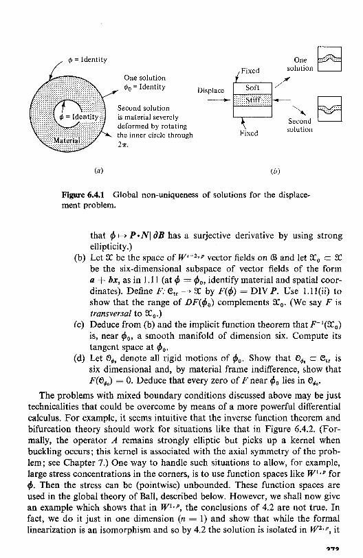
<I> = Identity
(a)
One solution <1>0 = Identity
Second solution is material severely deformed by rotating the inner circle through 2 ?T.
Displace -Fixed
One W solution L..:J
,-L----, / Soft /'
Fixed
(b)
~ Second solution
Figure 6.4.1 Global non-uniqueness of solutions for the displacement problem.
that ifJ ~ p.NI aB has a surjective derivative by using strong ellipticity.)
(b) Let X be the space of Ws-2,p vector fields on CB and let Xo c X be the six-dimensional subspace of vector fields of the form a + hx, as in 1.11 (at ifJ = ifJo, identify material and spatial coordinates). Define F: Gtr ~ X by F(ifJ) = DIV P. Use 1.11(ii) to show that the range of DF(ifJo) complements Xo. (We say F is transversal to Xo.)
(c) Deduce from (b) and the implicit function theorem that F-I(XO)
is, near ifJo, a smooth manifold of dimension six. Compute its tangent space at ifJo.
(d) Let 0"" denote all rigid motions of ifJo. Show that 0"" c Gtr is six dimensional and, by material frame indifference, show that F(0",,) = O. Deduce that every zero of F near ifJo lies in 0"".
The problems with mixed boundary conditions discussed above may be just technicalities that could be overcome by means of a more powerful differential calculus. For example, it seems intuitive that the inverse function theorem and bifurcation theory should work for situations like that in Figure 6.4.2. (Formally, the operator A remains strongly elliptic but picks up a kernel when buckling occurs; this kernel is associated with the axial symmetry of the problem; see Chapter 7.) One way to handle such situations to allow, for example, large stress concentrations in the corners, is to use function spaces like WI,p for ifJ. Then the stress can be (pointwise) unbounded. These function spaces are used in the global theory of Ball, described below. However, we shall now give an example which shows that in WI,P, the conclusions of 4.2 are not true. In fact, we do it just in one dimension (n = 1) and show that while the formal linearization is an isomorphism and so by 4.2 the solution is isolated in W2,P, it

w
/' /'
; i i ,. , • P- Po p+ Ux
Figure 6.4.2
is not isolated in WI,p. The difficulty is precisely that the nonlinear map is not CI. (See Morrey [1966] and Martini [1979] for related results.)
4.4 Example (Ball, Knops, and Marsden [1978]). We consider the displacement problem in one dimension, writing u for the nonlinear displacement: u = if> - Identity. On [0, I] we consider a stored energy function W(ux), suppose there are no external forces, and assume the boundary conditions u(O) = u(l) = O. Assume W is smooth and let p_ < 0 < p+ be such that
W'(p_) = W'(O) = W'(p+) and W"(O) > O.
(See Figure 6.4.2.) In W2,p (with the boundary conditions u(O) = 0, u(I) = 0), the trivial solu
tion Uo = O'is isolated because the map u ~ W(ux)x from W2,p to LP is smooth and its derivative at Uo is the linear isomorphism v ~ W"(O)v xx' Therefore, by the inverse function theorem, zeros of W(ux)x are isolated in W2,P, as above.
Note that the second variation of the energy V(u) = f W(ux) dx is positive
definite (relative to the HI = WI,2 topology) at Uo because if v is in W1.2 and vanishes at x = 0, I, then
::2 V(uo + EV)IE=O = W"(O) II v; dx > c II v Ilrvlo •.
Now we show that Uo is not isolated in WI,p. Given E > 0, let
for O<X<E,
for
for
.,. .. "

Slope = p+ Slope = p -!"--'-.30. __________ x
o €
Figure 6.4.3
(See Figure 6.4.3.) Since W'(uex) is constant, each u. is an extremal. Also
f I u.x - UOX Ip dx = f Ip+ Ip + flp_lplp+ Ip,
which tends to zero as f --? O. Thus Uo is not isolated in W1.p.
Remarks If W(p_) = W(p+) = W(O) and if W(p) > W(O) for allp, the same argument shows that there are absolute minima of V arbitrarily close to Uo in WI,P.
Phenomena like this seem to have first been noticed by Weierstrass. See Bolza [1904], footnote 1, p. 40. The "pathology" could possibly be eliminated by making good constitutive assumptions on W.
Now we turn to a discussion of global existence of solutions for the elastotatics problem. Thus, we wish to remove the restriction of locality in Theorem 4.2 and prove the existence of solutions for arbitrary loads. This is, then, a global nonlinear elliptic boundary value problem for a system. There have been at least four (overlapping) general methods used for dealing with such problems:
1. Convexity methods and monotone operators 2. Continuity methods 3. Topological methods and degree theory 4. Calculus of variations and minimizers
Method 1 considers an abstract operator F: 'Y --? X, where X is a Hilbert space and 'Y c X is a compactly embedded Banach space. We seek to solve F(u) = 1 assuming:
(i) F is CI ; F(O) = O. (ii) DF(u) is symmetric, so F(u) = 1 is the Euler-Lagrange operator of
J: 'Y --? IR,
J(u) = f <F(tu), u) dt - <I, u) (see Box 7.2, Chapter 1).
(iii) <DF(u)·h, h) > ell h II~ for all h E 'Y.
375
376 METHODS OF FUNCTIONAL ANALYSIS IN ELASTICITY CH. 6
Condition (iii) implies that J is strictly convex; if u -=1= v and 0 < t < 1, then J(tu + (I - t)v) < tJ(u) + (I - t)J(v), that J is bounded below and that F is strictly monotone:
<F(u) - F(v), u - v) > 0 if u -=1= v.
From this it is easy to see that solutions of F(u) = fare unique. Also, by selecting a minimizing sequence, one shows that it converges to a unique (generalized) solution of F(u) = f This idea is developed by Langenbach (1961] and is applied to elasticity by, for example, Beju [1971]. However, the convexity assumption (iii) is unsatisfactory for three good reasons: (1) it implies uniqueness of solutions and so precludes buckling; (2) convexity is incompatible with material frame indifference (Coleman and Noll [1959]); and (3) even in ranges where solutions may be unique, convexity need not hold, as is seen from the stretching experiment discussed in Ball [1977a].
Thus, while method 1 is mathematically very powerful and is appropriate for a number of important situations, it is not appropriate in its present form for three-dimensional nonlinear elasticity.
Gurtin and Spector [1979] (see also Gurtin [198Ia]) have looked for regions in the space of deformations where a convexity argument might be useful, and thereby have attempted to find sets of deformations in which uniqueness does hold.
Method 2 is based on the following "principle": to solve F(u) == j; we look at the range of F. Using the implicit function theorem as in 4.2, one can sometimes show that the range of F is open. Some additional estimates could be used to show the range is closed. By connectedness, this would imply that Range(F) = X, so F(u) = fwould be solvable. The following proposition illustrates the idea, although what is important is the method of proof. As far as we know, this technique has not yet been successfully applied in elasticity. 17
4.5 Proposition Suppose X, ~ are Banach spaces and F: ~ ----> X is a CI map and that at each point x E ~, DF(x) is an isomorphism of~ onto X. Assume that F is proper; that is, if C c X is compact, then F-I(C) c ~ is compact. Then F: ~ ----> X is onto.
Proof We can suppose without loss of generality that F(O) = O. Let x E X and consider the curve aft) = tx. By the inverse function theorem, there is a unique CI curve pCt) defined for 0 < t < f such that F(pCt)) = aCt). As in ordinary differential equations, extend p uniquely to its maximum domain of existence; say 0 < t < T < l. Let tn ----> T; then F(p(tn)) = a(tn) ----> aCT), so by the properness of F, p(tn) has a convergent subsequence, converging, say, to Yo. But as F is a local diffeomorphism in a neighborhood of Yo, the curve pCt) can
17For another proof and references, see Wu and Desoer [1972].

CH. 6 METHODS OF FUNCTIONAL ANALYSIS IN ELASTICITY 377
be defined up to and including T and beyond T if T < 1. Thus p is defined for o < t < 1 and F(p(I» = x. I
Problem 4.2 (a) Show that Fis proper if one has the estimate II DF(x)-l" > m > 0 for a constant m > O. (b) Show that Fin 4.5 is, in fact, one-toone by using the above proof and the fact that ~ is simply connected.
This proposition may be regarded as a primitive version of method 3, as well as an illustration of method 2. However, in method 3 the most common device used is not so much the use of curves in the domains and ranges of F, but rather to join the map F to another one Fo that can be understood; for example, Fo can be a linear map and the curve could be a straight line: F(t) = tF + (1 - t)Fo. The idea is to now invoke topological tools of degree theory to show that questions of solvability of F(u) = f can be continued back to those for solvability of Fo(u) = f The details are not appropriate for us to go into at this point; however, the method is powerful in a number of contexts. It allows multiple solutions (indeed it is very useful in bifurcation theory) and does not require any convexity assumptions. For general background and some applications, see Choquet-Bruhat, DeWitte, and Morette [1977]. For applications to rod and shell theory in elasticity, see Antman [1976a, b]. A global uniqueness theorem in the same spirit is given by Meisters and Olech [1963].
Now we turn to method 4, which we shall discuss a bit more extensively, following parts of Ball [l977a, b]. Let (B = n be a region in 1R3 with piecewise Cl boundary, and t/>: n -> 1R3 a typical deformation. Let W(F) be a given smooth stored energy function, 'OB a potential for the body forces, and '0, a potential for the tractions. As usual, the displacement will be prescribed t/> = t/>d on ad c an and the traction will be prescribed on a.: P·N = t. The energy functional whose critical points we seek is (see Section 5.1)
I(t/» = f. W(F) dV + f. 'OB dV + r '0, dA. n Q Ja,
In fact, we seek to minimize I(t/» over all t/> satisfying t/> = t/>d on ad' For dead loads we can take 'OB = -Beet> and '0, = -teet>, which are linear functions of t/>. The essential part of I(t/» is the stored energy function, so we shall assume that
I(t/» = L W(F) dVfor simplicity.
The method for minimizing I(t/» proceeds ~ccording to the following outline. On a suitable function space e of t/>'s:
(1) Show I is bounded below; then m = infl"'Ee 1(",) exists as a real number. Let t/>n be such that I(t/>n) -> m as n -> 00; that is, select a minimizing sequence (this is possible as m > - 00).
(2) Find a subsequence of t/>n that converges weakly; that is, t/>n ----> t/> (this notion is explained in Box 4.1).
(3) Show that I is weakly sequentially lower semicontinuous; that is, t/>n -~ t/> implies that I(t/» < lim infn~~ I(t/>n).

378 METHODS OF FUNCTIONAL ANALYSIS IN ELASTICITY CH. 6
If each of these steps can be effected, then rp is the minimizer of I. [Proof' Clearly I(rp) > m by definition of m. Also, if I(rpn) -> m, then lim infn~~ I(rpn) = m, so by 3, I(rp) < m. Thus I(rp) = m.]
In one dimension, this method can only work if W is convex. Indeed for this case, a theorem of Tonelli states that if I(rp) is weakly sequentially semicontinuous, then W is convex, and conversely. This is actually not difficult and is proved in Box 4.1. The related "relaxation theorem" is discussed in this box as well.
In elasticity, even in one dimension, two of the properties of minimizers rp that have to be carefully considered are smoothness and invertibility of rp. These are not simple; in one dimension, however, the situation is fairly well understood (mostly due to Antman [1976a, b]) and is discussed in Box 4.1.
In three dimensions, convexity of W is not necessary for this method to work. Indeed, it can be made to work under hypotheses that are reasonable for elasticity. The analog of Tonelli's result is due to Morrey [1952]; assume throughout that I W(F) I < C I + C2 1 Flp for constants C I and C2 , so I(rp) is defined for rp E WI,p(n).
4.6 Proposition If I(rp) = In W(F) dV is weakly sequentially lower semi
continuous on WI,p(n), then W is quasi-convex; that is, for all (constant) 3 x 3 matrices F with det F > 0 and all 1fI: n -> IR 3 that are C~ with compact support in n,
In W(F + VIfI(X» dV(X) > W(F) x volume(n). (QC)
This also implies strong ellipticity.
The proof is actually similar to Tonelli's theorem proved in Box 4.1, and reduces to it in one dimension, so is omitted. The inequality (QC) says essentially that if rph is a homogeneous deformation, I(rph) is a minimum among deformations rp with the same boundary conditions. Morrey also shows that (QC) and growth conditions imply sequential weak lower semicontinuity. However, this does not apply to elasticity because of the condition det F > 0 that we must be aware of.
To understand which stored energy functions give sequentially weakly lower semicontinuous (s.w.l.s) ['s, first consider the question of which ones give sequential weak continuity (s.w.c.). We state the following without proof:
4.6' Proposition (Ericksen, Edelen, Reshetnyak, Ball) Let W: Mmx n (the m X n matrices) ~ IR be continuous, I W(F) I < CI + C21 Flp (1 < p < 00), and let L(~) = W(Vrp); L: Wl.p -> Ll. Thefollowing are equivalent:
(1) Lis s.w.c. (2) L is a null Lagrangian; that is, L(rp + 1fI) = L(rp) for alllfl smooth with

CH. 6 METHODS OF FUNCTIONAL ANALYSIS IN ELASTICITY 379
compact support in n and all CI maps if>: n --> 1R3. (If W is smooth, this means the Euler-Lagrange equations for Ware identically satisfied for any if>.)
(3) W(F) = Constant + linear combination of r X r minors ofF for 1 < r < min(m, n).
For example, in three dimensions the null Lagrangians are W(F) = C + A·F + B·(adj F) + D(det F), where (adj F) is the matrix of cofactors of F and C, A, B, and D are constant. Some feeling for what is involved in 4.6 can be gained by working the following problem. (See Ball [1977a] for the complete proof.)
Problem 4.3 (Ball) Prove that det F is s.w.c. for 2 X 2 matrix functions by using the identity
det V'/' = ,/,1,/,2 _ ,/,1,/,2 = (,/,1'/'2) _ (,/,1'/'2) .,., "",1'11,2 '1',2'#',1 'II .,.,,2 .1 'I' '1',1 ,2 0
(This sort of trick is used in "compensated compactness"; cf. Tarter [1979].)
A good hypothesis on constitutive functions must be invariant under various transformations of coordinates. The following is one that is invariant under adding on null Lagrangians and the inversion transformation of fields if> ~ if>-I.
4.7 Definition W is called (strictly) polyconvex if there is a (strictly) convex function g: Mtx3 X M3 x3 X (0,00) --> IR such that W(F) = g(F, adj F, det F) for all FE Mt X3
•
One has the following chain of implications
Strict Convexity ==> Strict Polyconvexity ==> Quasi-Convexity ~
~ I -? Strong Ellipticity s.w .. s.
As remarked before, convexity is not a useful assumption. However, polyconvexity is valid for many specific materials, such as the Mooney-Rivlin and Ogden materials.
The following is a sample of one of Ball's results.
4.8 Theorem (Ball [I977b]) Suppose:
(HI) W is polyconvex. (H2) g(F, H, 0) < C + K(I FIP + I Hlq + 0') for constants K> 0, p > 2,
q > p/(p - 1), and r > 1. (H3) if (Fm Hn, On) --> (F, H, 0), then g(Fn' Hn> On) --> 00.
Let a = {if> E wI·p(n) I adj(Vif» E U, det Vif> E L',I(if» < 00, and if> = if>d on ad} and suppose a =1= 0. Then there exists a if> E a that minimizes I in a.
Sketch of Proof Take a minimizing sequence if>n. By (H2), we see that V if>n is bounded in Y, adj(Vif>n) is bounded in Lq, and det(Vif>n) is bounded in C. By

380 METHODS OF FUNCTIONAL ANALYSIS IN ELASTICITY CH. ~
the Poincare inequality and weak compactness of the unit ball we get a sub· sequence ¢I' such that
¢I' ~ ¢o in WI,P, adj V¢I' ~ H in U, and det V¢I' ~<5 in L'
By 4.6', adj and det are weakly continuous, so H= adj(V¢o) and <5 = det(V¢o)
Since g is convex, ¢ ~ /(¢) = fo g(F, adj F, det F) dV is s.w.l.s. so ¢o is thf
required minimizer. I
This sort of argument works well for the incompressible case, too, by weak continuity of det.
Open Problems
(a) Are minimizers weak solutions of the Euler-Lagrange equations?
(b) Are minimizers CI? (Ball [1980] has shown that strong ellipticity is necessary for regularity; however it may be sufficient if W(F)/IF 13 ---> 00 as IFI---> 00. Without such a condition, Ball [1982] has shown by means of a very important example involving cavitation that minimizers need not be smooth.)
(c) Are minimizers 1-1 deformations? (Using a result of Meisters and Olech [1963], Ball [1981] shows that this is true in the incompressible case.)
Box 4.1 Some Facts About Weak Convergence l8
In this box we shall state a few basic properties and examples of weak convergence; prove Tonelli's theorem and discuss the related relaxation theorem of L.e. Young; and discuss the proof of existence and regularity for one-dimensional problems.
These results only hint at the extensive literature on uses of the weak topology. Besides the work of Ball already cited, the articles of Tartar [1979] and DiPerna [1982] are indicative of current research in this area.
Ifa: is a Banach space and Xn is a sequence in OC, we write Xn ~ x and say Xn converges weakly to x if for all I E a:* (i.e., I: a: --> [R is continuous and linear), I(xn) --> lex) in [R. If a: = U([O, 1]), (1 < p < 00),
then Un ~ U means that
fol Unv dx --> f uV dx
for all v E U'[O, 1], where (lIp) + (lIp') = 1. This is because (U)* =
I 8We thank J. Ball for help with this box.

CH. 6 METHODS OF FUNCTIONAL ANALYSIS IN ELASTICITY 381
LP' (Riesz representation theorem). For X = L~ and we choose v E Lt, we speak of weak* convergence. Clearly ordinary convergence implies weak convergence.
Problem 4.4 Let ° < A < 1, a, b > 0, and Un = a on [0, Aln], Un = b on [Aln, lin], and repeat on every subinterval [i/n, (i + 1)ln] (i = 0, 1, ... , n - 1). Prove that Un ~ U = Aa + (I - A)b weak* in L~ [and hence in U[O, 1] (1 < p < 00)], but Un -h u.
In a reflexive separable Banach space X (such as WS,P(Q), 1 < p < 00) the unit ball is weakly sequentially compact; that is, if Un E X and II Un II = 1, then there is a subsequence Un. ~ U E X. The unit ball (or in fact any closed convex set) is weakly closed, so II U II < 1. (This result may be found in Yosida [1971], p. 125.)
Problem 4.5 In L2[0,2n] show that (l/--/"1t) sin nx = unCx) satisfies Un ~ 0, yet II Un II = 1. (Hint: Use the Riemann-Lebesgue lemma from Fourier series.)
Suppose W: [R+ --> [R is a given smooth function and for ifJ: [0, 1] -->
[R, ifJ' > 0 almost everywhere, define
I(ifJ) = f W(ifJ'(X» dX.
Assume I W(F) I < CI + C2 1 FIP so I maps {ifJ E WI,p I ifJ' > 0 a.e.} to [R.
4.9 Proposition (Tonelli) I is weakly sequentially lower semicontinuous (w.s.l.s.) if and only if W is convex.
Proof First of all, assume W is convex and let ifJn ~ ifJ in WI,p. By Mazur's theorem (see Yosida [1971]) there is a sequence of finite convex combinations, say IJIn = L, A~ifJ" L, A~ = 1 (0 < A, < 1) such that IJIn --> ifJ (strongly) in WI,p. By going to a further subsequence we can suppose IJI: --> IJI' a.e. By Fatou's lemma,
f W(ifJ'(X» dX < li~~nf f W(IJI~(X» dX.
By convexity of W, the right-hand side does not exceed
li~~nf ~ A~ f W(ifJ~(X» dX < li~~nf f W(ifJ~(X» dX.
Thus I is w.s.l.s. Conversely, assume I is w.s.l.s. Let ifJn(O) = ° and let ifJ:(X) = un(X),
given by Problem 4.4. By that problem, ifJn ~ ifJ(X) = (Aa + (I - A)b)X and W(ifJ~) ~ AW(a) + (1 - A) Web). Thus by w.s.l.s. I(ifJ) < lim infn~~

382 METHODS OF FUNCTIONAL ANALYSIS IN ELASTICITY CH. 6
I(¢n) becomes W(Aa + (1 - A)b) < AW(a) + (1 - A)W(b); that is, W is convex. I
Problem 4.6 Use this argument to prove that I is W.S.c. if and only if ¢(X) = aX + b for constants a and b. (This is the special case of Proposition 4.6 when n = 1 = m.)
In one dimension there is evidence that non-convex W's may be useful for describing phase transitions (Ericksen [1975]).19 However, in static experiments the non-convexity of W may not be observable. Indeed, the relaxation theorem of L.C. Young states that the minimum
of f W(¢'(X»dX is the same as that of f W*(¢'(X)dX, where W* is
the convex lower envelope of W (Figure 6.4.4). A convenient reference for this is Ekeland and Temam [1974]. In three dimensions the situation is far from settled.
w
--~----------~----------~¢/
Figure 6.4.4
Remaining in one dimension, consider the following hypotheses on W(X,F): .
(HI) W: [0, I] X (0,00) -> IR is CI. (H2) W(X, F) -> +00 as F -> 0+. (H3) W(X, F)/F -> 00 as F -> +00 uniformly in X. (H4) W(X, F) is convex in F.
19Phase transitions contemplated here may be seen if the polyethelene used in beer can packaging is stretched with your hands. It turns white, changing phase. Gentle heat will restore the original phase.
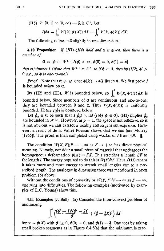
CH. 6 METHODS OF FUNCTIONAL ANALYSIS IN ELASTICITY 383
(H5) V: [0, 1] x [0, 00) --+ [R is CI. Let
J(¢) = f W(X, ¢'(X» dX + f VeX, ¢(X) dX.
The following refines 4.8 slightly in one dimension.
4.10 Proposition If (Hl)-(H4) hold and ~ is given, then there is a member of
a = {¢ E WLI I J(¢) < 00, ¢(O) = 0, ¢(1) = ~}
that minimizes 1. (Note that WI.I c Co, so if¢ E a, then by (H2), ¢' > ° a.e., so ¢ is one-lo-one.)
Proof Note that a =1= 0 since ¢(X) = ~X lies in a. We first prove J is bounded below on a.
By (H2) and (H3), W is bounded below, so f W(X, ¢'(X) dX is
bounded below. Since members of a are continuous and one-to-one, they are bounded between ° and ~. Thus VeX, ¢(X» is uniformly bounded. Hence J(¢) is bounded below.
Let ¢n E a be such that J(¢n) '\. inf {I(¢) I ¢ E a}. (H3) implies ¢n are bounded in WI.I. However, asp = 1, the space is not reflexive, so it is not obvious we can extract a weakly convergent subsequence. However, a result of de la Vallee Poussin shows that we can (see Morrey [1966]). The proof is then completed using w.s.l.s. of J from 4.9. I
The condition W(X, F)fF -> +00 as F -> +00 has direct physical meaning. Namely, consider a small piece of material that undergoes the homogeneous deformation ¢(X) = FX. This stretches a length IfF to the length I. The energy required to do this is W(F)I/F. Thus, (H3) means it takes more and more energy to stretch small lengths out to a prescribed length. The analogue in dimension three was mentioned in open problem (b) above.
Without the conditions of convexity or W(X, F)/F -> 00 as F -> 00, one runs into difficulties. The following examples (motivated by examples of L.C. Young) show this.
4.11 Examples (J. Ball) (a) Consider the (non-convex) problem of minimizing
II (¢' - 1)~\¢' - 2)2 + (¢ _ !X)2) dX
for x = ¢(X) with ¢' > 0, ¢(o) = 0, and ¢(l) =!. One sees by taking small broken segments as in Figure 6.4.5(a) that the minimum is zero.

384 METHODS OF FUNCTIONAL ANALYSIS IN ELASTICITY CH. 6
x x
Slope = 2
x
(a) (b)
Figure 6.4.5
However, the minimum can never be attained. Roughly, it is a line with infinitely many zig-zags. If W does not depend explicitly on X, then examples like this are not possible (cf. Aubert and Tahraoui [1979]).
(b) An example violating W(X, F)/F ~ 00 is
il (~, + cP' + cP) dX, cP(O) = 0, cP(1) = lX.
Direct calculation shows that the solution does not exist for lX > 2. See Figure 6.4.5(b). (This problem can be dealt with by making the transformation cP ~ cP-l-that is, by interchanging the roles of x and x.)
In one dimension there is more known about regularity than in three dimensions. In fact, we have the following (Antman [1976b]):
4.12 Proposition Suppose (HI), (H2), and (H5) hold and cP minimizes I in <t. Then the Euler-Lagrange equations
d~ Wp(X, cP'(X» = ViX, cP(X»
hold a.e. on [0, 1]. If, moreover, W is strictly convex in F and (H3) holds, then cP is 9 1 and cP' is bounded away from zero.
Proof The usual derivation of the Euler-Lagrange equations is not valid, so some care is needed; indeed, on <t, I is not differentiable. Let
nn = fX E [0, 1] 11/n < cP'(X) < n}.
Thus nn c nn+1 and .u([O, 1]\ Unn) = 0. Let v E L~, let Xn be the characteristic function of nn, and define If/(t, X) by
If/'(t, X) = cP'(X) + txiX)v(X), '1'(0) = 0.

CH. 6 METHODS OF FUNCTIONAL ANALYSIS IN ELASTICITY 385
We will show that (d/dt)/(If/(t, .» It=o exists. Since if> is a minimum, this is then zero. We have
+[[(If/(t, .» - [(If/(O, . »] =
..lll {W(X, if>'(X) + tx,,(X)v(X» - W(X, if>'(X»} dX t 0
+ + f {v(x, IX fif>'(X) + tx,,(X)V(X)]dX) - vex, if>(X)}dX
From the mean value theorem and the definition of 0" We see that the integrands are bounded, so we can pass to the limit t -> 0 by the dominated convergence theorem to get
o = it [(If/(t, .» It=o = in Wp(X, if>'(X»v(X) dX
+ t. V~(X, if>(X»(f x,,(X)v(X) dX) dX.
Integration by parts gives
o = t. Wp(X, if>'(X»)v(X) dX - t U: ViX, if>(X» dX) veX) dX.
Since v and n are arbitrary, we get
Wp(X, if>'(X» = r ViX, if>(X» dX a.e.
But this implies, by continuity of the integrand,
d~ Wp(X, if>'(X» = ViX, if>(X».
The second part follows by implicitly solving
Wp(X, if>'(X» = f v~Cf, if>(X» dX
for if>'. I
Box 4.2 Summary of Important Formulas for Section 6.4
Local Existence Theory for Elastostatics If about a given configuration if>o the linearized problem has unique
solutions (see Section 6.1, so the problem is not pure traction and no

386 METHODS OF FUNCTIONAL ANALYSIS IN ELASTICITY CH. 6
bifurcation occurs), and the boundaries of <B are smooth and no mixed boundary conditions with contiguous parts occur, then a small change in any of the data (boundary conditions, forces, or constitutive functions) produces a corresponding unique configuration if> in W',P, s > 3/p + 1 depending smoothly on the data.
Non-Applicability of the Inverse Function Theorem in Wl,P In W1,p solutions to the elastostatics equations need not be isolated,
even though the formal linearization of the equations is an isomorphism.
Convexity The assumptions of convexity and monotonicity are not appropriate
for the operators in three-dimensional elasticity.
Topological Methods Degree theory, Morse theory, and so on may be useful in three
dimensional elasticity, but so far have not been successfully applied because of technical difficulties. Minimizers
Global solutions in W1,p for elastostatics can be found by using weak convergence and minimizers. Under the assumption of polyconvexity and growth conditions on the stored energy function, minimizers exist. Their regularity is not known, except in one dimension.
6.S NONLINEAR ELASTODYNAMICS
This section surveys some results that are relevant to elastodynamics. The only part of this theory that is well understood is that dealing with semilinear equations-that is, equations that are linear plus lower-order nonlinear terms. This theory, due to Jorgens [1961] and Segal [1962], will be presented and applied to an example-the equations of a vibrating panel. The theory for quasi-linear equations-equations whose leading terms are nonlinear but depend linearly on the highest derivative-is appropriate for three-dimensional nonlinear elasticity. This will be briefly sketched, but much less is known. The primary difficulty is the problem of shock waves. The recent literature will be briefly discussed concerning this problem.
Elastostatics is imbedded in elastodynamics; each solution of the elastostatic equations is a fixed point for the equations of elastodynamics. Eventually, the dynamical context provides important additional information and intuition. For example, we may wish to know if the fixed points are stable, unstable, or are saddle points. We may also wish to find periodic orbits and examine their stability. For ordinary differential equations this leads to the large subject of dynamical systems (cf. Abraham and Marsden [1978] for more information and

CH. 6 METHODS OF FUNCTIONAL ANALYSIS IN ELASTICITY 387
references). For partial differential equations a good deal is known for semilinear equations and we shall give some examples in Section 6.6 and in Chapter 7. However, for the quasi-linear equations of three-dimensional elasticity, much less is known about qualitative dynamics.
Let us begin by recalling some general terminology (see Definition 3.3, Chapter 5).
A continuous local semiflow on a Banach space 'Y is a continuous map F: '!l c 'Y X IR+ ---+ 'Y, where '!l is open, such that: (i) 'Y X {OJ c '!l and F(x, 0) = x; and (ii) if (x, t) E '!l, then (x, t + s) E '!l if and only if (F(x, t), s) E '!l and in this case F(x, t + s) = F(F(x,t), s).
Suppose 'Y is continuously included in another Banach space X and G maps 'Y (or an open subset :D of 'Y) to X. We say G generates the semi flow jf for t > 0 and for each x E 'Y, F(x, t) is t-differentiable and
d dt F(x, t) = G(F(x, t»). (1)
As usual, if F(x, t) is defined for all t E IR, we call F a flow.
There is a slight philosophical difference with the linear case. For the latter, we started with F t : X -> X and constructed the generator by looking at where F t is t-differentiable at t = 0+. The domain of the generator is a Banach space 'Y with the graph norm, and Ft maps it to itself. This is compatible with the above definition. In the nonlinear case, it is better to start right off with Ft
defined on the smaller space 'Y. Then Ft mayor may not extend to all ofX. As we shall see, it does in the semilinear case. In this case we can use the phrase "G is the generator of F,."
Often we are given G and want to construct F(x, t) such that (1) holds. If an F exists, satisfying 5.1, we say the equations dxJdt = G(x) are well-posed. If solutioqs exist for all time t > 0 (or all t for flows), we say the equations generate global solutions.
A crucial part of well-posed ness is the continuous dependence of the solution F(x, t) on the initial data x-that is, continuity of the map x ~ F(x, t) from (an open subset of) 'Y to 'Y for each t > O. The satisfactory answer to such problems can depend on the choice of'Y made.
Sometimes it is necessary to study the case in which G depends explicitly on time. Then the flow is replaced by evolution operators Ft. s: 'Y -> 'Y satisfying F.,. = Identity and Ft,soFs.r = Ft.r • This is just as in Definition 6.5, Chapter 1. We replace (1) by
d dt Ft,.(x) = G(Ft..(x), t) (1 ')
with initial condition Fs..(x) = x (so "s" is the starting time). We begin now with a discussion of the semi linear case. The main method is
based on the Duhamel, or variation of constants, formula; namely, the fact

388 METHODS OF FUNCTIONAL ANALYSIS IN ELASTICITY
that the solution of
du f dt = Au + , u(O) = Uo
is u(t) = etAuo -+- s: e(t-slA!(s) ds.
CH. (
(See 2.l7(5) in Section 6.2.) If B depends on t and u, we conclude that the solution u(t) of
~~ = Au + B(t, u), u(O) = Uo (2)
satisfies the implicit equation
u(t) = etAuo + s: e(t-slAB(s, u(s» ds. (3)
The point now is that if B is a Lipschitz operator on the Banach space ~ (on which etA defines a semigroup), then the Picard iteration technique from ordinary differential equations applies to (3). If B is actually a C I map of ~ to ~, then we will show that solutions of (3) are in fact in :D(A) if U o E :D(A) and satisfy (2) in the strict sense.
The part of the analysis of (3) that is the same as that in ordinary differential equations is outlined in the following problem.
Prohlem 5.1 (Existence) Let A generate a Co semigroup on ~ of type (M, p) and let ~ = {u E C([O, toJ, ~) III u(t) - Uo II < R}, where to > ° and R > ° are constants and C([O, to], ~) is the set of continuous maps of [0, toJ to ~. Suppose B(t, u) is continuous and II B(t, u) II < Cp(t) if II U - Uo II < Rand ° < t < to. Define
T: ~ ---4 C([O, to], ~); (Tu)(t) = etAuo + J: e(t-slAB(s, u(s» ds.
(i) Show that if
II etAuo - Uo II + MePtoC fO Ip(s) Ids < R (0 < t < to),
then T maps ~ to ~. (ii) If B satisfies II B(t, uI) - B(t, u2) II < Kp(t) II UI - U2 II for UI and
U2 in the ball II U - Uo II <R and ° < t < to, where K is a (Lipschitz) constant (depending on R), then T satisfies
II TU I - Tu2 11 < f1" II UI - u2 11,
where the distance function on ~ c C([O, t 0]' ~) is
Ilu I - u2 11 = sup !lUI(t) - U2(t) II O:;E;t~to
and f1" is defined by
ito f1" = KMept• 0 Ip(s) Ids.

CH. 6 METHODS OF FUNCTIONAL ANALYSIS IN ELASTICITY 389
(iii) Deduce that jf IX < 1, then T has a unique fixed point by the contraction mapping principle (see Lemma l.3 of Section 4.1).
(iv) Show that instead of continuity of B, it is sufficient for B(t, u) to be V in t and Lipschitz in u.
Problem 5.2 (Uniqueness and Continuous Dependence on Initial Data)
(i) Prove Gronwall's inequality: if p is integrable on [a, b] and v is non-negative, bounded, and measurable on [a, b] and there is a constant C > 0 such that for all t E [a, b],
vet) < C + f Ip(s) 1 v(s) ds,
then vet) < C exp (f Ip(s) I) ds.
(See any book on ordinary differential equations; the solution is on p. 124 of Carroll [1969].)
(ii) In the setting of Problem 5.1, show that solutions of (3) satisfy
II u(t) II < MefJt• II U o II exp (CMe fJt• f: Ip(s) 1 dS)
and II u(t) - v(t) II < MefJt'li Uo - Vo II exp ( KMefJt• Dp(s)lds).
(iii) Use (ii) to show that solutions of (3) are Lipschitz functions of the initial data.
(iv) Use (ii) to give another proof of local uniqueness of solutions. (v) Prove that any two solutions of (3) are globally unique on their
common domain of definition if B is locally Lipschitz. (Hint: Show that the set of t where the two solutions coincide is both open and closed.)
Now we shall state the main theorem for semi linear equations in a version due to Segal [1962]. (Further important information is contained in subsequent corollaries.) To simplify the exposition, we shall assume B is independent of s. (The reader should do the general case.)
5.1 Theorem Let X be a Banach space and Ut a linear semigroup on X with generator A having domain ~(A). Suppose B: X -> X is a C k map (k > 1). Let G(u) = Au + B(u) on ~(A). Then (3) defines a unique local semiflow u(t) = F,(uo) on X (t > 0); Ft is a local flow if A generates a group. If Uo E ~(A), then Ft(uo) E ~(A) and (1) holds. Moreover,for each fixed t, Ft is a C k mapping of an open set in X to X.
Proof Problems 5.1 and 5.2 show that (3) defines a local flow and that Ft is locally Lipschitz. We next show that Ft(x) is differentiable in x. To do so one can appeal to a general theorem on ordinary differential equations in Hale [1969] (Theorem 3.2, p. 7). We can also show that F t is Cl by a direct calculation

390 METHODS OF FUNCTIONAL ANALYSIS IN ELASTICITY CH. 6
as follows. For x E ~, let 8lx) E (B(~) (the bounded linear operators from ~ to ~) satisfy the linearized equations:
8t(x) = U, + I: Ut_sDB(F.(x»·8.(x) ds.
8,(x) is defined as long as F;(x) is defined. It is easy to check that t ~ 8lx) is continuous in the strong operator topology and that (for fixed t), x ~ 8,(x) is norm continuous. We claim that DF,(x) = 8lx), which w;ll thus prove Ft is CI. Let
Then
AlX,h)=11 I: Ut_s{B(F.(x + h» - B(Fs(x» - DB(F.(x».8.(x)'h} ds ll
< Mexp(Plt I){DI B(F.(x+h»-B(F.(x»-DB(F.(x»·[Fix+h) - F.(x) lid
+ I:IIDB(Fix».[Fix + h) - Fix) - 8ix).h]llds}.
Thus, given E > 0, there is a J > ° such that II h II < J implies
A,(x, h) < (const.)· {II h II E + s: A.(x, h) ds}.
Hence (by Gronwall's inequality), A,(x, h) < CCt) II h II E. Hence, by definition of the derivative, DF,(x) = O,(x). Thus F, is C I. An induction argument can be used to show F, is C k
•
Now we prove that F, maps 1>(A) to 1>(A) and
d dt F,(uo) = G(F,(uo»
is continuous in t. Let Uo E 1>(A). Then, setting u(t) = F;(uo), (3) gives
1 1 1 (' h[u(t + h) - u(t)J = h(Ut+huO - U,u o) + h Jo (U,+h-s - U,_s)B(u(s»ds
1 (,+h + h Jo U,+h_sB(U(s» ds
1 1 f'+h = h [Uiu(t» - u(t)] + h, U,+h_sB(U(s» ds. (4)
The second term approaches B(u(t» as h ---> O. Indeed,
ill ft+h II 1 f'+h h t Ut+h-sB(u(s» ds - B(u(t» < h t II Ut+h_.B(U(s» - B(u(t» lids
1 f'+h < h t II U,+h_sB(U(s» - Ut+h_sB(u(t» II ds
1 f'+h + h t II U'+h_.B(U(t» - B(u(t» lids

CH. 6 METHODS OF FUNCTIONAL ANALYSIS IN ELASTICITY 391
I It+h < h . C(t) • . t II B(u(s» - B(u(t» II ds
I It+h + h t II Ut+h_sB(u(t» - B(u(t» lids
and each term ----> 0 as h ----> O. It follows that Ft(uo) is right differentiable at t = 0 and has derivative G(uo).
To establish the formula at t =1= 0 we first prove that u(t) E ~(A). But
1 1 h (Ft+hu O - Ftuo) = h (FtFhuO - F,uo)
has a limit as h ----> 0 since F, is of class CI. Hence, from (4),
! [Uiu(t» - u(t)]
has a limit as h ----> O. Thus, u(t) E ~(A). It follows that
d dt Fluo) = G(Ft(uo» = DFt(uo)·G(uo)·
Since the right derivative is continuous, the ordinary (two-sided) derivative exists as well. I
Next we give a criterion for global existence.
5.2 Proposition Let the hypotheses of 5.1 hold. Suppose u(t) is a solution of (3) defined for 0 < t < T and that II B(u(t» II is an integrable function of t on [0, T]. Then u(t) can be continued to a solution for 0 < t < T + f for f > o.
Proof For 0 < t, s < T, we have from (3),
II u(t) - u(s) II < II etAuo - esAuo II + II f e(t-<)AB(u(r» II d-r
< IIetAuo - eSAuol1 +MePT f" B(u(-r»lI d-r
Thus u(t) is a Cauchy sequence as t ----> T, so converges, to, say uT. The local existence theory applied in a neighborhood of UT shows the time of existence is uniformly bounded away from zero as t ----> T; so the result follows. I
Here is an example of how this works.
5.3 Corollary Suppose B satisfies II B(u) II < C + KII u II for constants C and K. Then the semijlow Ft is global-that is, is defined for all t > o.
Proof Fix T> 0 and let u(t) solve (3) for 0 < t < T. Then
II u(t) II < MePTlluo II + s: MePT(C + Kllu(-r)II)d-r.

392 METHODS OF FUNCTIONAL ANALYSIS IN ELASTICITY CH. 6
From Grownwall's inequality (Problem 5.2),
II u(t) II < [MePT II UO II + CT] exp(KMePT)
so II u(t) II and hence II B(u(t» II are bounded for ° < t < T. Thus u can be extended beyond T by 5.2. Hence u is defined for all t > 0. I
Prohlem 5.3 Prove a global existence theorem if
II B(t, u) II < p(t)[C + KII u II], where pet) is V on every finite interval.
Another way of obtaining global existence is through energy estimates. That is, if the equations are Hamiltonian (or are related to a Hamiltonian system), there may be a conserved (or decreasing) energy function that can be used to obtain the needed estimate in 5.2. We give an example in the following:
5.4 Corollary Suppose the conditions of Theorem 5.1 hold. Suppose, moreover, that there is a Cl function H: X -- IR such that:
(i) there is a monotone increasing function if>: [a, 00) -- [0, 00), where [a, 00) -=> Range H, satisfying II x II < if>(H(x»;
Oi) there is a constant K > ° such that ifu(t) satisfies (3), then
(iii)
ft H(u(t» < KH(u(t».
Then Ft(uo) is defined for all t > ° and Uo E X; that is, the semiflow is global.
If, in addition, H is bounded on bounded sets and
ft H(u(t» < ° if II u(t) II > E,
then any solution of (3) remains uniformly bounded in X for all time; that is, given Uo E ~(A), there is a constant C = C(uo) such that II u(t) II < C for all t > 0.
Proof By (ii), H(u(t» < H(uo) exp(Kt) so by (i), II u(t) II < if>(H(uo) exp(Kt». Thus, global existence follows by 5.2. Let HB = sup [H(u) III u II < B}, so, by (iii), H(u(t» < max [H(uo), HB}. Hence, by (i), we can take C = if>(max[H(uo), HB}). I
Next we have a criterion for asymptotic stability of a fixed point Xo; that is, FtCxo) = Xo and Flx) -- Xo as t -- +00 for all x E X. (See Theorem 4.1 of Chapter 7 for the use of spectral methods to obtain a related result.)
5.5 Proposition Let (i) and (U) of 5.4 hold, and suppose G(xo) = 0; that is, Xo is a fixed point, and:
(iii') There is a continuous monotone function f: [0, 00) -- [0, 00), locally Lipschitz on (0, 00) such that
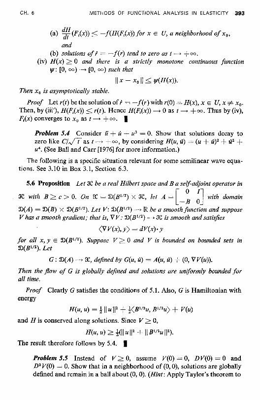
CH. 6 METHODS OF FUNCTIONAL ANALYSIS IN ELASTICITY 393
(a) ~~ (F,(x)) < -f(H(F,(x)) for x E U, a neighborhood of x o,
and (b) solutions ofr = -fer) tend to zero as t ---> +00.
(iv) H(x) > ° and there is a strictly monotone continuous function lfI: [0, (0) ---> [0, (0) such that
II x - Xo II < lfI(H(x)).
Then Xo is asymptotically stable.
Proof Let ret) be the solution of r = - f(r) with reO) = H(x), x E U, X *" Xo.
Then, by (iii'), H(F,(x)) < ret). Hence H(F,(x)) ---> ° as t ---> +00. Thus by (iv), F,(x) converges to Xo as t ---> +00. I
Problem 5.4 Consider ii + u + u3 = 0. Show that solutions decay to zero like C/~t as t ---> +00, by considering H(u, u) = (u + U)2 + u2 + u4
• (See Ball and Carr [1976] for more information.)
The following is a specific situation relevant for some semi linear wave equations. See 3.10 in Box 3.1, Section 6.3.
5.6 Proposition Let JC be a real Hilbert space and B a self-adjoint operator in
JC with B > c > 0. On X = ~(Bl/2) X JC, let A = [ _ ~ ~J with domain
~(A) = ~(B) X ~(Bl/2). Let V: ~(Bl/2) ---> IR be a smooth function and suppose V has a smooth gradient; that is, V V: ~(Bl/2) ---> JC is smooth and satisfies
<VV(x),y) = dV(x)· y
for all x, y E ~(Bl/2). Suppose V > ° and V is bounded on bounded sets in ~(Bl/2). Let
G: ~(A) ---> X, defined by G(u, u) = A(u, u) + (0, VV(u)).
Then the flow of G is globally defined and solutions are uniformly bounded for all time.
Proof Clearly G satisfies the conditions of 5.1. Also, G is Hamiltonian with energy
H(u, u) = t II u W + t(Bl/2U, Bl/2U) + V(u)
and H is conserved along solutions. Since V > 0,
H(u, u) > t(lIuW + II Bl/2U In The result therefore follows by 5.4. I
Problem 5.5 Instead of V >0, assume V(O) = 0, D V(O) = ° and D2 V(O) = 0. Show that in a neighborhood of (0, 0), solutions are globally defined and remain in a ball about (0,0). (Hint: Apply Taylor's theorem to

394 METHODS OF FUNCTIONAL ANALYSIS IN ELASTICITY CH. €
H to show that in a neighborhood of (0,0), cI11 (u, u) W < H(u, u) < Cz " (u, u) W for constants C I and Cz.)
Problem 5.6 (Regularity) Let 5.1 hold and suppose that B: ~(Ak-l)----> ~(Ak-l) is C1-I, 1= 1, ... ,k - 1, where ~(Ak-l) has the graph norm. Prove that F, maps ~(Ak-I) to itself and is Ck-I.
Problem 5.7 (Singular Case) Let A generate a Co semi group on OC and let :D(A) have the graph norm. Suppose B: ~(A) ----> OC is CI and the tangent of B, TB: (u, v) 1---)0 (u, DB(u)·v) extent to a CI map of~(A) X OC to ~(A) X OC. Then G = A + B generates a unique local CI flow. (Hint: Apply 5.1 to the operator TG(u, v) = (0, v) + TB(u, v); the first component of this flow gives the flow of G; cf. Segal [1962].)
We will now give two applications of this theory. The first is to semilinear non-linear wave equations and the second is to a problem of panel flutter. The first is perhaps not directly relevant to elasticity, but it is a topic of current interest and illustrates the methods well. (See Reed [1976] for similar results from a different point of view. For a recent spectacular application of the semilinear theory, see Eardley and Moncrief [1982].)
5.7 Example (Semilinear Wave Equation) We consider the following equation for rp(x, t) E IR, where x E IRn and t E IR:
~:t = VZif> - m2rp - grpp,} (5)
if>(x, 0) and ~(x, 0) given
where p > 2 is an integer and g E IR is a constant. (One can also consider this problem on complete Riemannian manifolds, but we stick to IRn for simplicity.) To obtain the results, essential use is made of the Sobolev spaces HS(IRn
) and the Sobolev inequalities. To obtain global solutions, these inequalities must be applied with care. The relevant facts we need were given in Box 1.1, Section 6.1.
The results for Equation (5) are summarized as follows:
(i) For n = I, 2, m > 0, g > 0, p an odd integer, and s > I, Equation (5) has unique global solutions in HS+I(IRn
, IR) X HS(IRn, IR) for any initial
data in this space. (ii) For n = 3, m > 0, g > 0, and p = 3, the conclusion (i) remains valid.
(iii) For n = 1, 2, m > 0, any g, and any p, there are unique global solutions as in (i) if the initial data is small enough in HI X V norm. The same holdsfor n = 3 ifp < 4.
(iv) For any n, m, g, p, there are unique solutions local in time in HS+ I(IRn, IR) X HS(IR
n, IR) if s + I > n12.
Note: From hyperbolicity arguments (Courant and Hilbert [1962]) it follows that if we start with COO data with compact support, the solution will be COO with compact support as well.

CH. 6 METHODS OF FUNCTIONAL ANALYSIS IN ELASTICITY 395
To establish (i) and (ii), we use Proposition 5.6 (with a slight modification if m = 0), and to prove (iii) we use Problem 5.5, and to prove (iv) we use Theorem 5.1. We shall give the details for case (ii).
First, suppose m > O. Then as was discussed in Section 6.3 the KleinGordon operator
A=[~~m2 ~J is skew-adjoint on HI X P with the energy norm, which is equivalent to the usual Sobolev norm. We set
V:HI ----->IR,
Here is the key fact:
V(¢) = K r ¢4 dx. 4 J~3
Lemma 1 V is a well-defined smooth map with defivative
DV(¢)'1jI =g r ¢3Ij1dx. J~3
Proof From the Sobolev-Nirenberg-Gagliardo inequality (see Box 1.1), there is a positive constant C such that for ¢ E P(1R 3
),
II ¢J Ib < C II V ¢ 11~211 ¢J Ill,a for 2 <p< 6 and a = 3·(± - lip). In particular, we have the estimate
//¢Jlb < C//¢//Hl for 2 <p< 6. The main case, p = 6, was proved in Proposition 1.16. Taking p = 4 we see that V is well defined. Consider
From the Schwartz inequality,
Hence '0 is a continuous multilinear map; so is C=. Hence V is as well, and so the lemma follows. I
Lemma 2 Set Y: HI -----> P; Y(¢J) = (_g¢3). Then Y is a C= map and the conditions of Proposition 5.6 hold, with A as above, JC = P, and V V = Y.
Proof Since £6 CHI, Y is well defined. Consider ID: H I X H I X HI -----> L2, ID(¢JI' ¢2' ¢3) = IIl=I ¢i' Then by HOlder's inequality,
Thus ID and hence Y is smooth. A straightforward calculation shows that V V = Y. I

396 METHODS OF FUNCTIONAL ANALYSIS IN ELASTICITY CH. 6
That solutions which start in HS+ I X HS for s > 2 stay in that space follows by regularity (Problem 5.6). We ask the reader to supply the details.
The case m = ° may be dealt with as follows. Using the usual norm on HI X V, conservation of energy and v> ° implies that II ViP IlL' + II ~ ilL' is bounded, say, by M. But this implies that II ViP ilL' + II iP ilL' + II ~ ilL' < M + tMil iPo ilL" so the (HI X U)-norm is bounded on finite t-intervals. Thus we again get our result.
The result (iv) is perhaps the easiest of all. Indeed, for s > n/2, HS(fRn, fR) is a
ring: II/gliH' < CII/IIH'IIgIIH" so multiplication is smooth. (See 1.17 in Box 6.1.1.) Therefore, we can apply Theorem 5.1 directly because any polynomial Y on H' will be smooth.
5.8 Example (Panel Flutter) The linear problem was considered in Box 3.2. (See Figure 6.3.1.) Here we consider the nonlinear problem. The equations are
(X/i/'II + Villi - {r + IC f (V'(t, e»2 de + u f (v'(t, e)i/(t, e» de} v"
+ pv' + ",Jfi ov + v = o. (6)
(See Dowell [1975] and Holmes [l977a].) As in Box 3.l, . = a/at, I = a/ax, and we have included viscoelastic structural damping terms (x, u as well as aerodynamic damping ",Jfi 0; IC represents nonlinear (membrane) stiffness, p the dynamic pressure, and r an in-plane tensile load. We have boundary conditions at x = 0, 1 that might typically be simply supported (v = (v + (XV)" = 0) or clamped (v = v' = 0). To be specific, let us choose the simply supported condition.
To proceed with the methods above, we first write (6) in the form (2), choosing as our basic space OC = H;([O, 1]) X V([O, 1]), where Hi denotes H2 functions in [0, 1] that vanish at 0, 1. Set II (v, v) IIoc = (II v W + II v" W)I/2, where II· II denotes the usual V-norm. This is equivalent to the usual norm because of the boundary conditions. In fact, the two Poincare-type inequalities II v' W > 11:2 11 v Wand II v" II > 11:4 11 v W may be checked using Fourier series. Define
A = where (0 I) {CV = -V'II' + rv" - pv', CD' Dv = _(XV"" - ",Jp ov.
(7)
The domain ~(A) of A consists of all pairs (v, v) E OC such that v E Hi, v + (Xv E H4, and v" + (Xv" = ° at x = 0, 1. Define the nonlinear operator B(v, v) = (0, [IC II v' 112 + u<v', V')]V"), where <.) denotes the V inner product; so (6) can be rewritten as
~: = Ax + B(x) = G(x), where x = (v, v) and x(t) E ~(A). (8)
By Proposition 3.11 in Box 3.2, Section 6.2, A generates a semigroup on OC. In one dimension HI forms a ring; so as in the previous example, B: OC -> OC is

CH. 6 METHODS OF FUNCTIONAL ANALYSIS IN ELASTICITY 397
a Coo mapping bounded on bounded sets. Thus, by Theorem 5.1, Equations (6) generate a local semiflow on oc. We claim that this semiflow is global. To see this, we temporarily omit the dissipative terms in (6), namely, we consider
v"" - {r + 1C ( (v'(t, e))2 de} v" + ii = o. As in Problem 3.6, Section 6.3, this is Hamiltonian with
H(v, v) = !llvW + !llv"JIl + ~ Ilv'W + ~ IIv'W·
For the full equation (6) we find by a simple calculation that
~~ = -p(v', v) - -/ pollvW - o:llV"JIl - ull(v, v)JI2.
< -p<v', v) < p Ilv' IllIv II <tp(11 v' JI2 + Ilv W)·
For II v' II large enough,
H(v, v) > Gil (v, v) Iii. [Note that r can be < 0; write
£11 v' 112 + !£ II v' II' = !£ II v' JI2 {II v' 112 + 2r} 2 4 4 1C
to see this.] Thus, for II v' II large, hypotheses (i) and (ii) of 5.4 are satisfied, and so we have global solutions. We shall return to this example again in Chapter 7.
Problem 5.8 (Parks [1966], Holmes and Marsden [1978aD Let H(v, v) = !{-/Ji 0 II v JI2 + 0: II v" JIl + 2(v, v) + (uI2) II v' W} and let XCv, v) = H(v, v) + vH(v, v), where v = (-/po + 0:1C4)/2. If p2 < (-/ po + 0:1C 4)2 X
(r + p2), show that dXldt < 0 along non-zero solutions. Use 5.5 to show that in these circumstances solutions tend to (0,0) as t -> +00.
While the above theory does apply to a number of special situations in elasticity involving rod and plate approximations, it does not apply to the "full" theory of nonlinear elasticity, even in one dimension. Here the equations have the form
u = A(t, u)u + J(t, u) (0 < t < T, u(O) = uo), (9)
the point being that the linear operator A depends on u. For example, onedimensional elasticity has this form:
Such equations in which the highest derivatives occur linearly, but possibly multiplied by functions of lower derivatives, are called quasi-linear. The remainder of this section discusses the theory for these equations. This theory began
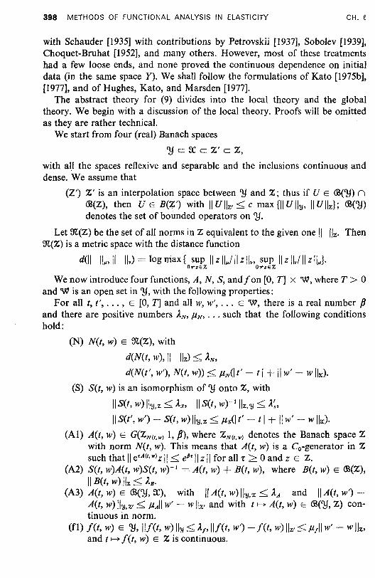
398 METHODS OF FUNCTIONAL ANALYSIS IN ELASTICITY CH. E
with Schauder [1935J with contributions by Petrovskii [1937J, Sobolev [1939], Choquet-Bruhat [1952J, and many others. However, most of these treatments had a few loose ends, and none proved the continuous dependence on initial data (in the same space Y). We shall follow the formulations of Kato [1975bJ, [1977], and of Hughes, Kato, and Marsden [1977].
The abstract theory for (9) divides into the local theory and the global theory. We begin with a discussion of the local theory. Proofs will be omitted as they are rather technical.
We start from four (real) Banach spaces
'Y c X c Z' c z, with all the spaces reflexive and separable and the inclusions continuous and dense. We assume that
(Z') Z' is an interpolation space between 'Y and Z; thus if V E <B('Y) n <B(Z), then V E B(Z') with II Vllz' < c max {II VII')!, II VllzJ; <B('Y) denotes the set of bounded operators on 'Y.
Let m:(Z) be the set of all norms in Z equivalent to the given one II liz. Then m:(Z) is a metric space with the distance function
d(1I II", II IIv) = log max { sup liz 11,,/ II z II .. sup II z IIvI II z II,,}· O,ozEZ O,ozEZ
We now introduce four functions, A, N, S, andJon [0, T] x 'W, where T > ° and'W is an open set in 'Y, with the following properties:
For all t, t', ... , E [0, TJ and all w, w', ... E 'W, there is a real number p and there are positive numbers AN, J.lN, ... such that the following conditions hold:
(N) N(t, w) E m:(Z), with
d(N(t, w), II liz) < AN,
d(N(t', w'), N(t, w» < J.lN(1 t' - t I + II w' - w Ib)' (S) Set, w) is an isomorphism of'Y onto Z, with
IIS(t, w)II')!,z < As, IIS(t, w)-lllz,,)! < A:,
II Set', w') - Set, w) 1I')!,z < J.lsCl t' - t I + II w' - w IbJ (AI) A(t, w) E G(ZN(t,W) I, P), where ZN(t,w) denotes the Banach space Z
with norm N(t, w). This means that A(t, w) is a Co-generator in Z such that II eTA(t,w) z II < efi< II z II for all 't" > ° and z E Z.
(A2) Set, w)A(t, w)S(t, W)-l = A(t, w) + B(t, w), where B(t, w) E <B(Z), II B(t, w) liz < AB •
(A3) A(t, w) E <B('Y, X), with II A(t, w) 1I')!,oc < AA and II A(t, w') -A(t, w) 1I')!,z' < J.lAIl w' - w liz' and with t 1---+ A(t, w) E <B('Y, Z) continuous in norm.
(fl) J(t, w) E 'Y, IIJ(t, w) II')! < A" IIJ(t, w') - J(t, w) liz' < J.l,1I w' - w liz, and t 1---+ J(t, w) E Z is continuous.

CH. 6 METHODS OF FUNCTIONAL ANALYSIS IN ELASTICITY 399
Remarks (i) If N(t, w) = const. = 1/ liz, condition (N) is redundant. If Set, w) = const. = S, condition (S) is trivial. If both are assumed, and X = Z' = Z, we have the case of Kato [1975b].
(ii) In most applications we can choose Z' = Z and/or Z' = X. (iii) The paper of Hughes, Kato, and Marsden [1977] had an additional
condition (A4) that was then shown to be redundant in Kato [1977]. (iv) The possibility of dropping (S) and related refinements are discussed in
Graff [1981] and Altman [1982].
5.9 Theorem Let conditions (Z/), (N), (8), (AI) to (A3), and (fl) be satified. Then there are positive constants p' and T' < T such that if Uo E 'Y with II UO - Yo 11')1 < p', then (9) has a unique solution u on [0, T'] with
u E CO([O, T']; 'W) n C 1([0, T']; X).
Here p' depends only on AN, As, A~, and R = dist (Yo, 1/\'W), while T'may depend on all the constants p, AN, PN, ... and R. When Uo varies in 1/ subject to II uo - Yo 11')/ < p', the map Uo ~ u(t) is Lipschitz continuous in the Z'-norm, uniformly in t E [0, T'].
To establish well-posed ness, we have to strengthen some of the assumptions. We assume the following conditions:
(B) II B(t, w') - B(t, w) liz < PB II w' - w 11')1' (f2) Ilf(t, w') - f(t, w) II 1/ < pi II w' - w 11')1'
5.10 Theorem Let conditions (Z'), (N), (8), (AI) to (A3), (B), (fl), and (f2) be satisfied, where Set, w) is assumed to be independent of w. Then there is a positive constant T" < T'such that when Uo varies in 1/ subject to II Uo - Yo 11')1 < p', the map uo ~ u(t) given by Theorem 5.9 is continuous in the 1/-norm, uniformly in t E [0, T"].
As in Kato [1975b], one can prove a similar continuity theorem when not only the initial value uo but also the functions N, A, andJare varied; that is, the solution is "stable" when the equations themselves are varied. Variation of S is discussed in Graff [1981]. In summary, Theorem 5.10 guarantees the existence of (locally defined) evolution operators Ft .• : 1/ -> 1/ that are continuous in all variables.
The idea behind the proofs of the Theorems 5.9 and 5.10 is to fix a curve vet), in 1/ satisfing v(O) = uo and let u(t) be the solution of the "frozen coefficient problem"
u = A(t, v)u + J(t, v), u(O) = uo,
which is guaranteed by linear theory (Kato [1970], [1973]). This defines a map <II: v ~ u and we look for a fixed point of <II. In a suitable function space and for T' sufficiently small, <II is in fact a contraction, so has a unique fixed point.
However, it is not so simple to prove that u depends continuously on uo and detailed estimates from the linear theory are needed. The proof more or less

400 METHODS OF FUNCTIONAL ANALYSIS IN ELASTICITY CH. 6
has to be delicate since the dependence on Uo is not locally Lipschitz in general. For details of these proofs, we refer to Kato [1975b], [1977] and Hughes, Kato, and Marsden [1977]. The continuous dependence of the solution on Uo leads us to investigate if it is smooth in any sense. This is important in Hamiltonian systems, as we saw in Proposition 3.4, Chapter 5. This is explored in Box 5.1 below.
Next we give some specific systems to which 5.10 applies. These will be nonlinear versions of first-order symmetric hyperbolic systems and second-order hyperbolic systems. Each of these applies to nonlinear elasticity; to verify the hypotheses (details of which are omitted) one uses the linear theory presented in Theorems 3.1 (for the second-order version) and 3.19 of Section 6.3. We shall treat these equations in all of IRm as the machinery needed for boundary value problems is yet more complex (see Kato [1977] and Box 5.2 below).
5.11 Example (Quasi-linear Symmetric Hyperbolic Systems) Consider the equation
au {!-, au ao(t, x, u)-a = k.J ait , x, u)-a . + aCt, x, u). t j~ I Xl
(10)
for x E IRm, t E IR, u(t, x) E IRN, and ai' a real N X N matrices. We assume:
(i) s> 1m + 1 and ao, a are of class Cs+I in the variables t, x, u (possibly locally defined in u);
(ii) there are constant matrices aj, a OO such that
ai - aj, a - a OO E C([O, T], HO(lRm) n L 00([0, T], Hs(lRm»
ao - aD E Lip([O, T], H S-I(lRm», locally uniformly in u;
(iii) ai' (j = 0, ... , m) are symmetric;
(j = 0, 1, ... , m),
(iv) ao(t IX, u) > cJ for some c > 0 for all x and locally in t, u.
Under these conditions, the hypotheses of Theorem 5.10 hold with
x = HS-l(lRm),
S = (1 - Ll)s/z,
Thus (10) generates a unique continuous evolution system F t •s on 'Y.
5.12 Example (Second-order Quasi-linear Hyperbolic Systems) Consider the equation
aZu m dZu aoo(t, s, u, VU)-a Z = I: aJt, x, u, VU)-a i a j t l.j~l X X
m azu + 2 ~ aolt, x, u, Vu) at axi + aCt, x, u, Vu). (1 I)

CH.6 METHODS OF FUNCTIONAL ANALYSIS IN ELASTICITY 401
Here
We assume:
(i) S> (mI2) + 1 and a"p, a are of class cs+1 in all variables (possibly locally defined in u);
(ii) there are constant matrices a';p, aOO such that
a"p - a';p, a - aOO E Lip([O, T]; Hs-I(IRm» c Loo([O, T]; Hs(IRm»,
locally uniformly in u;
(iii) a"p is symmetric; (iv) aoo(t, x, u) > cI for some c > 0; (v) strong ellipticity. There is an € > 0 such that
I'~I alit, x, u)c!/ei > € C~ WJ2) (a matrix inequality) for all l; = (e l , ••. ,em) E IRm, x E IRm, and locally in t, u.
Under these conditions, Theorem 5.10 holds with
X = Hs(IRm) X Hs-I(IRm),
Z = Z' = HI(lRm) X HO(IRm),
'Y = HS+I(IRm) X Hs(lRm),
S = (1 - A)s/2 X (1 - A)s!2,
A(t) = ( _. [ 0 a' ] -f [ a J). aOO 1: ali axl axi aOO 2 1: aO} ax}
Thus (11) generates a unique continuous evolution system on 'Y.
From either 5.11 or 5.12 we conclude that the equations of nonlinear elastodynamics generate a unique continuous local evolution system on the space of if>, ~, which are sufficiently smooth; if> is at least C2 and ~ is C I.
There are several difficulties with theorems of this type: (A). The existence is only local in time. (B). The function spaces are too restrictive to allow shocks and other discontinuities.
With regard to (A), some global results for (11) have been proved by Klainermann [1978] (and simplified by Shatah [1982]) in four or higher dimensions for small initial data. However, these global Properties are not true in three dimensions (John [1979]). Much work has been done on (B), but the success is very limited. In fact, the problem in one dimension is not settled. Simple dissipative mechanisms sometimes relieve the situation, as is discussed below.
A few selected topics of current interest related to difficulties (A) and (B) are as follows:

402 METHODS OF FUNCTIONAL ANALYSIS IN ELASTICITY CH. ~
1. Lax [1964] proved the non-existence of global smooth solutions to
assuming that a" never vanishes. Equation (12) is studied by writing it as a system of conservation laws:
where w = U x and v = ut •
2. The assumption aU =F 0 is unrealistic for nonlinear elasticity. Indeed it is reasonable that a stress-strain function a(ux ) should satisfy a(p) -> + 00 as p -> +00 and a(p) -> -00 as p -> 0+. Strong ellipticity is the assertion that a'(p) > ~ > O. This does not imply that aU never vanishes. This hypothesis was overcome by MacCamy and Mizel [1967] under realistic conditions on a for the displacement problem on [0, 1] (representing longitudinal displacements of a bar). These results have been improved by Klainermann and Majda [1980] who show that singularities develop in finite time for arbitrarily small initial data under rather general hypotheses. The results are still, however, one dimensional.
3. A general existence theorem for weak solutions of (12) was proved by Glimm [1965] and Dafermos [1973]. The crucial difficulty is in selecting out the "correct" solution by imposing an entropy condition. This problem has been recast into the framework of nonlinear contractive semigroups by several authors, such as Quinn [1971] and Crandall [1972].
Glimm constructed solutions in the class of functions of bounded variation by exploiting the classical solution to the Riemann problem for shocks. The proof that the scheme converges involves probabilistic considerations. DiPerna [1982], using ideas of Tartar [1979], obtains solutions in L= as limits of solutions of a viscoelastic problem as the viscosity tends to zero. DiPerna's results involve acceptable hypotheses on the stress a and impose correct entropy conditions on the solutions. (The solutions are not known to be of bounded variation).
4. Much has been done on equations of the form (12) with a dissipative mechanism added on. For example, viscoelastic-type dissipation is considered in MacCamy [1977], Matsumura and Nishida [1980] and Potier-Ferry [1980] and thermoeleastic dissipation is considered in Coleman and Gurtin [1965J and Slemrod [1981]. It is proved that smooth initial data with small norm has a global solution. Dafermos [1982], using the ideas in Andrews [1980], shows smooth, global existence for arbitrarily large initial data for thermoviscoelasticity.
5. The viscoelastic equations UtI = a(uxL + Uxxt without the assumption of strong ellipticity are shown to have unique global weak solutions in Andrews [1980]. This is of interest since, as we mentioned in the previous section, a a without the restriction a' > 0 may be relevant to phase transitions.

CH. 6 METHODS OF FUNCTIONAL ANALYSIS IN ELASTICITY 403
Box 5.1 Differentiability of Evolution Operators
This box gives an abstract theorem which shows that in some sense the evolution operators Ft .• for a system of the type (1)' are differentiable. This is of interest for quasi-linear systems and applies, in particular, to the situation of 5.10. For semilinear systems, Ft•s is smooth in the usual sense, as we already proved in Theorem 5.1. However, the example U t + uUx = 0 shows that F t : HS --> Hs is not even locally Lipschitz, although F t : HS --> Hs-l is differentiable (see Kato [I 975aJ), so the situation is more subtle for quasi-linear hyperbolic systems. Despite this, there is a notion of differentiability that is adequate for Proposition 3.4, Chapter 5, for example. For quasi-linear parabolic systems, the evolution operator will be smooth in the usual sense. For more details, see Marsden and McCracken [1976], Dorroh and Graff [1979], and Graff [1981].
First, we give the notion of differentiability appropriate for the generator. Let a: and cy be Banach spaces with cy c a: continuously and densely included. Let 'll c cy be open and f: 'll --> a: be a given mapping. We say f is generator-differentiable if for each x E 'll there is a bounded linear operator Df(x): cy --> a: such that
Ilf(x + h) - f(x) - Df(x)·h Ilx --> 0 II h Ilx
as II h II'Y --> O. If/is generator-differentiable and x ~ Df(x) E CB(CY, a:) is norm continuous, we call f Cl generator-differentiable. Notice that this is stronger than Cl in the Frechet sense. Iffis generator-differentiable and
Ilf(x + h) - f(x) - Df(x)·h II xiii h Ilx is uniformly bounded for x and x + h in some cy neighborhood of each point, we say thatfis locally uniformly generator-differentiable.
Most concrete examples can be checked using the following proposition:
5.13 Proposition Suppose f: 'll c cy --> a: is of class C2, and locally in the cy topology
II D2f(x)(h, h) Ilx x ~ II h II'Y II h Ilx
is bounded. Then f is locally uniformly C 1 generator-differentiable.
This follows easily from the identity
f(x + h) - f(x) - Df(x)·h =:, fa' fa' D2f(x + sth)(h, h) ds dt.

404 METHODS OF FUNCTIONAL ANALYSIS IN ELASTICITY CH. 6
Next, we turn to the appropriate notion for the evolution operators. A map g: 'U c 'Y ---> X is called flow-differentiable if it is generator
differentiable and Dg(x), for each x E '\1, extends to a bounded operator X to X. Flow-differentiable maps obey a chain rule. For example, if gl: 'Y ---> 'Y, g2: 'Y ---> 'Y and each is flow-differentiable (as maps of 'Y to X) and are continuous from Y to 'Y, then g2 o g1 is flow-differentiable with, of course,
The proof of this fact is routine. In particular, one can apply the chain rule to Ft.soFs.r = Ft.s if each Ft .• is flow-differentiable. Differentiating this in sat s = r gives the backwards equation:
a as Ft..(x) = -DFt . .(x)·G(x).
Differentiation in r at r = s gives
DFtjx)·G(x) = G(Ftjx)),
the flow invariance of the generator.
Problem 5.9 Use the method of Proposition 2.7, Section 6.2 to show that integral curves are unique if (l)' has an evolution operator that is flow-differentiable.
For the following theorem we assume these hypotheses: Y c X is continuously and densely included and F t •s is a continuous evolution system on an open subset:D c 'Y and is generated by a map G(t)::D --->
X. Also, we assume:
(HI) G(t): :D c Y ---> X is locally uniformly CI generator-differentiable. Its derivative is denoted DxG(t, x) and is assumed strongly continuous in t.
(H2) For x E :D, s > 0, let T x •s be the lifetime of x beyond s: that is, T x.s = sup [t > s I Ft.s(x) is defined}. Assume there is a strongly continuous linear evolution system [Ux.S(r, a) I ° <a < r < T x •s} in X whose X-infinitesimal generator is an extension of [DxG(t,Ft.sx) E B(Y,X)IO<t<Tx.s}; that is, if y E 'Y, then
a~+ Ux.s(r, a)·y L. = DxG(r, F •. .(x))·y.
(Sufficient conditions for (H2) are given in Kato [1973].)

CH. 6 METHODS OF FUNCTIONAL ANALYSIS IN ELASTICITY 405
5.14 Theorem Under the hypotheses above, Ft.s is flow-differentiable at x and, in fact,
DFt./x) = ux.s(t, s).
Proof Define rp,(x, y) = rpU, x, y) by
G(t, x) - G(t, y) = DxG(t, y)·(x - y) + II x - y Ilxrpt(x, y)
(or zero if x = y) and notice that by local uniformity, II rp(t, x, y) Ilx is uniformly bounded if x and yare <y-close. By joint continutity of Ft.sCx), for 0 < t < Tx.s> II rp(t, Ftjy), Ft./x)) Ilx is bounded for 0 < s < T if II x - y 11'1:1 is sufficiently small.
By construction, we have the equation
d dt Ftjx) = G[Ft.lx)] (0 < s < t < Tx,s> x E ~).
Let wet, s) = Ftjy) - Ft.sCx)
so that aw(t, s) ( ( « at = G t, Ft.s y)) - G t,Ft.s x))
= DxG(t, Ft./x))w(t, s) + II w(t, s) Ilxrp(t, F"sY, F,.sx).
Since DxG(t, F"sx)·w(t, s) is continuous in t, s with values in a:, and writing U = ux.s, we have the backwards differential equation:
a ( ) ( ) _ ) aw(a, s) ) aa U t, a w a, s - U(t, a aa - U(t, a)DxG(a, F"jx)).w(a, s
= U(t, 0')·11 w(a, s) Ilxrp(a, F"jy), F"jx)).
Hence, integrating from a = s to a = t,
w(t, s) = U(t, s)(y - x) + s: U(t, a) II w(a, s) Ilxrp(a, F"jy), F"jx)) dO'.
Let II U(-/:, a) Ilx,x < M, and II rpCa, F"jy), F"jx)) Ilx < M 2 , (0 < s < a < l' < T). Thus, by Gronwall's inequality,
IIw(t,s)llx < MleM,M2Tlly - xlix = M 3 11y - xlix. In other words,
IIF,.ly) - F,.sCx) - Vet, s)(y - x) Ilx Ily - xlix .
< MI M 3 s: II rp(a, F",s(Y), F"jx)) Ilx dO'.
From the Lebesgue bounded convergence theorem, we conclude that Ft •s
is flow-differentiable at x and DFt.sCx) = U(t, s); (rp(t, F, . .(y), Ft.sex)) is strongly measurable in s since rp(x, y) is continuous for x "* y.) I

406 METHODS OF FUNCTIONAL ANALYSIS IN ELASTICITY
Box 5.2 Remarks on Continuity in the Initial Data for the Initial Boundary Value Prohlem for Quasi-linear Systems
CH. (
As stated, Example 5.12 applies only to an elastic body filling all of space. For the initial boundary value problem, Kato [1977] has shown local existence and uniqueness, but the continuous dependence on the initial data is not yet known. The method is to replace CY by the domain of a power of A, such as A3. The major complication that needs to be dealt with is the compatability conditions and the possibility that the domains of powers of A will be time dependent, even though that of A is not. All of this is caused by the degree of smoothness required in the methods and the dependence of A on u.
We shall now sketch a method that may be used in proving the continuous dependence in certain cases. 20 Write the equations this way:
U + ~(u) = 0, Uo = ifJ, where ~(u) = A(u)·u and we have dropped the termf(u) for simplicity. Suppose that the boundary conditions are written
B(u) = 0, u E :D(~).
If we seek solutions in the domain of[A(uW, then the compatability conditions for the initial data are obtained by differentiating B(u) = 0 twice:
(i) B(ifJ) = 0; (ii) B'(ifJ)'~(ifJ) = 0;
(iii) B"(ifJ)·(IJ(ifJ), IJ(ifJ)) + B'(ifJ)·IJ('(ifJ)·IJ(ifJ) = O.
The difficulty is that even if B(ifJ) = 0 are linear boundary conditions, this is a nonlinear space of functions in which we seek the solution. Let C denote the space of functions satisfying the compatability conditions. It seems natural to try to show C is a smooth manifold. We assume B itself is linear for simplicity and assume our function spaces are Hilbert spaces, so closed subspaces will split.
5.15 Proposition Let ifJ E C and assume: (a) B is surjective; (b) the linear boundary value problem
~'(ifJ)' '" = p,
has a solution", for any p; and
E·", = 0,
20M. Ortiz has pointed out to us that this result may also be provable using product formula methods. C. Dafermos has noted that for the second order hyperbolic case, which includes elasticity, classical energy and elliptic estimates may give the result.

CH. 6 METHODS OF FUNCTIONAL ANALYSIS IN ELASTICITY 407
(c) the linear boundary value problem
S!!"(¢)(S!!(¢), IJI) + (S!!'(¢»21J1 = p
B'S!!'(¢)'IJI = 0
has a solution IJI for any p.
B'IJI = 0,
Then C is a smooth manifold in the neighborhood of ¢. Proof Let C 1 = Ker B, the "first" boundary conditions. Map
¢ E C 1 ~ B(¢).S!!(¢) = B·S!!(¢).
This has derivative at ¢ given by IJI ~ B·S!!'(¢)·IJI. Since B is surjective and S!!'(¢): Ker B --> (range space) is surjective by (b), this map has a surjective derivative, so C2 = {¢ E C 1 lB· S!!(¢) = O} is a submanifold of C 1 with tangent space T",C2 = {IJI: BIJI = 0 and B'S!!'(¢)'IJI = OJ, by the implicit function theorem.
Finally, map
C2 --> (range space), -¢ ~ B.S!!'(¢)·S!!(¢),
which has the derivative IJI ~ B· [S!!"(¢)(S!!(¢), IJI) + (S!!'(¢»2 ·IJIJ. Thus, by assumption (c), this is surjective on T",C2 • Thus,
C3 = {¢ E C2 IB.S!!'(¢)·S!!(¢) = O} = C
is a submanifold by the implicit function theorem. I
We want to solve
du + S!!(u) = 0 dt
for u(t) E C with a given initial condition ¢ E C. To do so, we can use the local diffeomorphism
ct>: C ---> (linear space) = 1',
with ct>( ¢) = ¢ mapping a neighborhood of ¢ in C to a ball about ¢ in a linear space obtained from the proof above. (So ct> is only defined implicitly.) Let v = ct>(u). Thus
q'l}. = ct>'(u)du = ct>'(ct>-l(V»'( -S!!(ct>-l(V») dt dt '
so v satisfies the modified equation
dv -cli + S!!(v) = 0,
where ~(v) = ct>'(ct>-l(V»' S!!(ct>-l(V». (In geometry notation, ~ = ct>*S!!.) If the modified problem is well-posed, then clearly the original one is as well. We can choose Y = {IJII BIJI = 0, B· S!!'(¢)'IJI = 0 and

408 METHODS OF FUNCTIONAL ANALYSIS IN ELASTICITY CH. 6
B· [W"(¢)(W(¢), '1') + (W'(¢))21j1] = OJ and let <I> be the projection of C onto Y; see Figure 6.5.1.
All functions u
'- y'C
'Y = Functions satisfying the linearized compatibility
conditions at </>.
Figure 6.5.1
Now let W have the form W(u) = A(u)· u. Since <I> is a linear projection, the equation
§'rev) = <I>·A(<I>-I(V))·<I>-I(V)
is still quasi-linear. It seems reasonable to ask that the abstract quasilinear Theorem 5.11 applies to the new system W. If it does, then continuous dependence for the initial boundary value problem follows.
Box 5.3 Remarks on Incompressible Elasticity
In Example 4.6 Section 5.4 we remarked that the configuration space for incompressible elasticity is evoh the deformations ¢ with J = 1. (This requires careful interpretation if ¢ is not CI.) The equations of motion are modified by replacing the first Piola-Kirchhofl" stress P / =
PRer(aWjaPA ) by PRer(aWjaPA ) + Jp(F-l)aA, wherep is a scalar func
tion to be determined by the condition of incompressibility. A fact discovered by Ebin and Marsden [1970] is that this extra term Ppresur.(¢'~) = Jp(F-I) in material coordinates is a C~ function of (¢, ~) in the HS X HS (and hence Hs+1 X HS) topology. (In fact, there is one order of smoothing in the H s+ 1 X H s topology; see also Cantor [1975b].) This remark enables one to deduce that in all of space the equations of incompressible elasticity are well-posed as a consequence of that for the compressible equations. (One can use, for example, Marsden

CH. 6 METHODS OF FUNCTIONAL ANALYSIS IN ELASTICITY 409
[1981] for this, or the abstract Theorem 5.10.) Again the boundary value problem requires further technical requirements.
The smoothness (as a function of if» of the pressure term Ppressure in the stress seems not to have been exploited fully. For example, it may help with studies of weak (Hopf) solutions in fluid mechanics. In particular, it may help to prove additional regularity or uniqueness of these solutions. In general (as has been emphasized by J. Ball) it is a good idea in fluid mechanics not to forget that material coordinates could be very useful and natural in studies of existence and uniqueness.
We conclude with a few remarks on the incompressible limit, based on Rubin and Ungar [1957], Ebin [1977], and Klainerman and Majda [1918}. If the "incompressible pressure" p is replaced by a constitutive law Pk(p), where (dPkldp) = k, so 11k is the compressibility, then a potential Vk is added to our Hamiltonian which has the property:
Vk(if» = 0 if if> E eVO\ and Vk(if» --> 00 as k --> +00
if if> 1:- evol '
In such a case, it is intuitively clear from conservation of energy that this ought to force compressible solutions with initial data in eval to converge to the incompressible solutions as k --> 00.
Such convergence in the linear case can be proved by the TrotttrKato theorem (see Section 6.2). Kato [1977] has proved analogues of this for non-linear equations that, following Theorem 5.10, are applicable to nonlinear e1astodynamics. These approximation theorems may now be used in the proofs given by Ebin [1977]. Although all the details have not been checked, it seems fairly clear that this method will enable one to prove the convergence of solutions in the incompressible limit, at least for a short time. (See Klainerman and Kohn [1982].)
We also mention that the smoothness of the operator Ppressure and the convergence of the constraining forces as k --> 00 should enable one to give a simple proof of convergence of solutions of the stationary problem merely by employing the implicit function theorem. Rostamian [1978} gives some related results.
Problem 5.10 Formulate the notion of the "rigid limit" by considering SO(3) c e and letting the rigidity --> 00.
Problem 5.11 A compressible fluid may be regarded as a special case of elasticity, with stored energy function W(F) = h(det F), where h is a strictly convex function.
(a) Show that the first Piola-Kirchhoff stress is P = h'(det F) adj F (or (J = h'(det F)/) and the elasticity tensor is

410 METHODS OF FUNCTIONAL ANALYSIS IN ELASTICITY CH.6
A = h"(det F) adj F ® adj F + h'(det F) • a(a:~ F).
(b) Show explicitly in two dimensions using suitable coordinates, that A is not strongly elliptic.
(c) Despite (b), show that the equations are locally wellposed by using Ebin (1977] or a direct argument to check the abstract hypotheses of 5.9 and 5.10.
Box 5.4 Summary of Important Formulas for Section 6.5
Semiflow on 11 Autonomous: F,: 11 -> 11; Fo = Identity, F,+s = F,oFs Time-dependent: F,.s: 11 ---> 11; Fs •s = Identity, F,.s = F,.roFr.s
Generator
it F,(x) = G(F,(x» (autonomous)
it F, . .<x) = G(F,..(x), t) (time-dependent)
Variation oj Constants Formula
If du/dt = Au + J(t), then u(t) = e'Auo + t eC'-S)AJ(s) ds.
Semilinear Equations If A is a linear generator on X and B: X ----> X is Coo, then G(x) =
Ax + B(x) generates a smooth local semi flow on X. Ifan a priori bound for II B(x) II can be found, the semiflow is global.
Panel Flutter The equations
a:i;"" + v"" - {r + "Ii v' iii, + a<v', V')L'}V" + pv' + .-.Iii ov + v = ° on [0, 1]
with boundary conditions
v = (v + !Xv)" = 0 at x = 0, I
generate a unique smooth global semi flow on Hi X L2.
Quasilinear Equations Hyperbolic (symmetric first-order or strongly elliptic second-order)
systems define local flows on spaces of sufficiently smooth functions.

CH. 6 METHODS OF FUNCTIONAL ANALYSIS IN ELASTICITY 411
The evolution operators are differentiable in the technical sense of "flow differentiability. "
Little is known about global solutions for quasi-linear equations, although some results that necessarily involve entropy conditions are known in one dimension.
6.6 THE ENERGY CRITERION
The energy criterion states that minima of the potential energy are dynamically stable. A major problem in elasticity (that is not yet settled) is to find conditions appropriate to nonlinear elasticity under which this criterion can be proved as a theorem. The purpose of this section is to discuss some of what is known about the problem for nonlinear elasticity. The linearized case has been discussed in Theorem 3.5. There are both positive and negative results concerning the criterion for nonlinear elasticity; examples discussed below show that the criterion is probably false as a sweeping general criterion; but there are theorems to indicate that these counterexamples can be eliminated with reasonable hypotheses.
The energy criterion has been extensively discussed in the literature. It seems to have first been explicitly recognized as a genuine difficulty by Koiter [1945], [1965b], [1976a], although it has been very successfully used in engineering for much longer. Relevant mathematical theory is closely related to bifurcation theory and goes back at least to Poincare [1885]. A detailed account of the history and basic results available up until 1973 are contained in Knops and Wilkes [1973], which should be consulted by any readers who have a serious interest in pursuing this subject. Some of the other more recent references that are important are (chronologically): Ericksen [1966a, b], Coleman [1973], Naghdi and Trapp [1973], Knops, Levine, and Payne [1974], Gurtin [1975], Payne and Sattinger [1975], Mejlbro [1976], Ball, Knops, and Marsden [1978], Knops and Payne [1978], Ball and Marsden [1980], and Ball [1982]. There are many references that deal with stability in the context of bifurcation theory such as Ziegler [1968] and Thompson and Hunt [1973]; these aspects will be discussed in Chapter 7.
The difficulties with the energy criterion for conservative infinite-dimensional quasi-linear systems may be genuine ones. Some possible alternatives are:
0) Use some kind of averaging technique to mask the higher frequency motions, thereby making semilinear techniques applicable (see 6.10 below). As far as we know this possibility has not been explored.
(ii) Employ a dissipative mechanism in addition to a conservative minimum of the potential. It is possible that a suitable mechanism will move the

412 METHODS OF FUNCTIONAL ANALYSIS IN ELASTICITY CH. I
spectrum into the left half-plane so that Liapunov's theorem (4.1 0
Chapter 7) becomes applicable. In Potier-Ferry [1980] this is estah lished for viscoelasticity of Kelvin-Voigt type, as in Propositior 3.12, Section 6.3, generalizing the work of Dafermos [1969], [1976] For a dissipative mechanism of thermal type, see Slemrod [1981]. Fo] both thermal and viscous dissipation, see Dafermos [1982].
The contents of this section are as follows.
1. First we give (in 6.3) sufficient conditions for validity of the energy cri· terion. This involves the notion of a potential well.
2. The applicability of this theorem to elasticity is then criticized and exam· pIes are presented to show that it is at best difficult to satisfy the hypotheses.
3. A positive result is proved showing that potential wells can be obtained in Wl,P (spaces in which the existence of dynamics is questionable).
4. Semilinear equations are discussed and the validity of the energy criterion is proved under acceptable hypotheses in this case.
5. Some discussion of the role of dissipative mechanisms is given.
Let us begin with sufficient conditions for the validity of the energy criterion. This version goes back at least to Lagrange and Dirichlet and is satisfactory for finite degree of freedom systems and for some infinite degree of freedom systems (the semi linear ones), as we shall see.
The general context is that of Hamiltonian systems with energy of the form kinetic-plus-potential. To be a bit more concrete than the context of Section 5.3, let us adopt the following set-up:
(a) X and cy are Banach spaces. (b) K: cy --> IR, called a kinetic energy function, is a given continuous
function that satisfies K(y) > 0, with K(y) = ° only if y = 0. (c) V: X --> IR is a given continuous potential energy function. Let H:
X x cy --> IR be defined by H(x, y) = K(y) + Vex).
We are contemplating the dynamical system associated with Hamilton's equations, so let us write x for y, although it need not be a time derivative. We consider the following two assumptions.
6.1 Assumptions Let Xo E X be fixed. For each 11 > 0 and b> 0, let the K-neighborhood about (xo, 0) of radius (11, b) be defined by
S'1'~ = {(x, x) E X X cy III x - XO II < 11 and K(x) < b}.
Assume:
(Sl) There is an 110 > 0, bo > 0, and 'C > 0 and a continuous local semiflow F, defined on S'10'~O for 0 < t < 'C such that (i) (xo, 0) is a fixed point for F,-that is, F,(xo, 0) = (xo, D)-and (ii) H(x(t), x(t» < H(x(O) X(O» for all (x(O), x(O» E S'10'~O' where (x(t), x(t» =
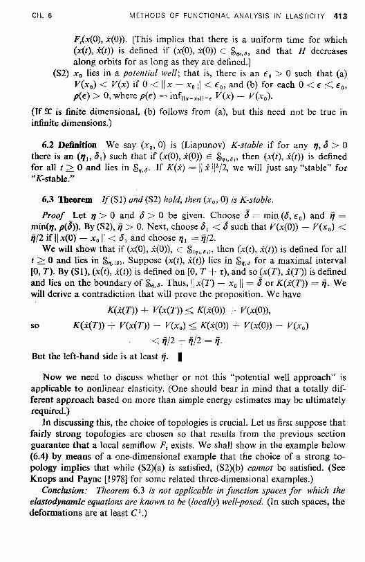
CH. 6 METHODS OF FUNCTIONAL ANALYSIS IN ELASTICITY 413
F,(x(O), x(O». [This implies that there is a uniform time for which (x(!), x(t») is defined if (x(O), x(O» E S~o.Jo and that H decreases along orbits for as long as they are defined.]
(S2) Xo lies in a potential well; that is, there is an f 0 > 0 such that (a) V(xo) < Vex) if 0 < II x - XO II < fo, and (b) for each 0 < f < fo,
peE) > 0, where p(f) = infllx-xoll~€ Vex) - V(xo).
(If ~ is finite dimensional, (b) follows from (a), but this need not be true in infinite dimensions.)
6.2 Definition We say (xo, 0) is (Liapunov) K-stable if for any 17, ~ > 0 there is an (111, ~I) such that if (x(O), x(O» E S~l.Jl' then (x(t), x(t» is defined for all t > 0 and lies in S~.J. If K(x) = \I x W12, we will just say "stable" for "K-stable. "
6.3 Theorem 1f(SI) and (S2) hold, then (xo, 0) is K-stable.
Proof Let 11 > 0 and ~ > 0 be given. Choose J = min (£5, fo) and fi = min(l1, p(J)). By (S2), fi > O. Next, choose £5 1 < J such that V(x(O) - V(x o) < fil2 if 1\ x(O) - XO II < £5 1 and choose 111 = fi12.
We will show that if (x(O), x(O», E S(~l.Jl» then (x(t), x(t» is defined for all t > 0 and lies in S~.(J). Suppose (x(t), x(t» lies in S~.J for a maximal interval [0, T). By (S1), (x(t), x(t») is defined on [0, T + -r), and so (x(T), x(T)) is defined and lies on the boundary of S~.J. Thus, II x(T) - XO II = J or K(x(T) = fi. We will derive a contradiction that will prove the proposition. We have
K(x(T» + V(x(T) < K(x(O» + V(x(O»,
so K(x(T) + V(x(T» - V(xo) < K(x(O») + V(x(O) - V(xo)
< fil2 + fil2 = fi· But the left-hand side is at least fi· I
Now we need to discuss whether or not this "potential well approach" is applicable to nonlinear elasticity. (One should bear in mind that a totally different approach based on more than simple energy estimates may be ultimately required.)
In discussing this, the choice of topologies is crucial. Let us first suppose that fairly strong topologies are chosen so that results from the previous section guarantee that a local semiflow F, exists. We shall show in the example below (6.4) by means of a one-dimensional example that the choice of a strong topology implies that while (S2)(a) is satisfied, (S2)(b) cannot be satisfied. (See Knops and Payne [1978] for some related three-dimensional examples.)
Conclusion: Theorem 6.3 is not applicable in function spaces for which the elastodynamic equations are known to be (locally) well-posed. (In such spaces, the deformations are at least C 1 .)
414 METHODS OF FUNCTIONAL ANALYSIS IN ELASTICITY CH. 6
6.4 Example (Ball, Knops, and Marsden [1978]) Let ill = [0, 1] and consider displacements ¢: [0, 1] -> IR with ¢(o) = ° and ¢(1) = 2 > ° prescribed.
The potential is V(¢) = f W(¢x) dX. Suppose that W is C2, W'(l) = 0, and
W"(l) > O. Then ¢o(X) = 2X is an extremal for V. Let a: be a Banach space continuously included in W I ,=.
1. Under these conditions, (S2)(a) holds; that is, there is an £ > ° such that if 0 < II ¢ - ¢o Ilx < £, then V(¢) > V(¢o). That is, ¢o is a strict local minimum for V.
Proof This follows from the fact that l is a local minimum of Wand that the topology on a: is as strong as that of W I ,=. I
2. We necessarily have failure of (S2)(b) in a:; that is,
inf V(¢) = V(¢o)' II¢-¢ollx~'
Proof By Taylor's theorem,
V(¢) - V(¢o) = f (W(¢x) - W(2» dX
= f f (1 - s)W"(s¢x + (1 - s)2) ds dX.
Thus, as s¢x is uniformly bounded (a: c W I ,=) and W" is continuous, there is C > 0 such that
V(¢) - V(¢o) < C f (¢x - 2)2 dX.
However, the topology on a: is strictly stronger than the Wl,2 topology, and so
inf 51 (¢x - 2)2 dX = 0, II¢-¢ollx~' 0
which proves our claims. I
3. In Wl,p one cannot necessarily conclude that ,po is a local minimum even though the second variation of Vat ¢o is positive-definite.
Proof The example W(¢x) = t(¢i - ¢i) shows that in any WI.P neighborhood of ¢o, V(¢) can be unbounded below. I
There is a Morse lemma available which enables one to verify S2(a) and to bring V into a normal form. See Tromba [1976], Golubitsky and Marsden [1983] and Buchner, Marsden and Schecter [1983]. The hypotheses of this theorem are verified in item 1 above but fail in item 3.
A more important example of the failure of the energy criterion has been constructed by Ball [1982]. He shows that a sphere undergoing a radial tension will eventually rupture due to cavitation. This is done within the framework of

CH. 6 METHODS OF FUNCTIONAL ANALYSIS IN ELASTICITY 415
minimizers in Wl,p discussed in Section 6.4. The "rupture" solution corresponds to a change in topology from CB, a sphere, to cp(CB), a hollow sphere; clearly cP cannot be continuous at the origin, but one can find such a cP in Wl,p for a suitable p < 3. Formally, the energy criterion would say that the trivial unruptured radial solution is stable, but in fact it is unstable to rupturing, a phenomenon not "detected" by the criterion.
Since the hypothesis (S2)(b) fails if the topology is too strong, it is natural to ask if it is true in weaker topologies, especially WI,p. In fact, we shall prove that with reasonable h}potheses in WI,P, (S2)(b) follows from (S2)(a). However, as there is no existence theorem for elastodynamics in Wl,p, (SI) is unknown (and presumably is a difficult issue).
The heart of the argument already occurs in one dimension, so we consider it first.
Let W: [R + -> [R be a strictly convex C 1 function satisfying the growth condition
Co + 0(;01 s Ip < W(s)
for constants Co > 0, 0(;0 > 0, p > 1. Fix A> ° and let Wl'P denote those cP E WI,P([O, 1]) such that cp(O) = 0, and cp(l) = A. Define V: Wl'P --> [0,00] by
V(cp) = fa' W(CPx) dX
and let
II cp III.p = (II CPx Ip dXYIP
Let CPo (X) = AX, so CPo E Wp and V(CPo) = W(A).
6.5 Proposition (Ball and Marsden [1980]) V has a potential well at CPo; that is, (a) V(cp) > V(cpo)for cP *- CPo, cp E WI'P, and (b) for f > 0,
inf V(cp) > V(CPo)' 114>-4>011".=<
4> EWX'
Proof (a) Integration by parts and the boundary conditions give
° = fa' W'(A)(CPx - (CPoh) dX
and so
Sal [W(CPx) - W(A)] dX
= fa' {W(cpx) - W(A) - W'(A)(CPx - A)} dX > ° since W lies strictly above its tangent line. This proves (a).
(b) We prove (b) by contradiction. By (a),
inf V(cp) > V(CPo)· 114>-</>0111 •• =<
416 METHODS OF FUNCTIONAL ANALYSIS IN ELASTICITY CH. (
Suppose equality held. Then there would be a squence ifJ~ EO Wl'P satisfying
II ifJ~ - ifJo II1.p = E (1) and
(2)
From (1) we can extract a weakly convergent subsequence of the ifJ~ (See Box 4.1, Section 6.4). Thus we may suppose that ifJ~ -' ~ in W!'p. I
6.6 Lemma ~ = ifJo.
Proof By weak lower sequential continuity of V (Tonelli's theorem; see Box 4.1),
By (2) we get
so by part (a), ~ = ifJo' I
6.7 Lemma lfv~ --> v in LP,
( W(v) dX < 00 and (W(vn) dX ---> ( W(v) dX,
then there is a subsequence V~k -~ v a.e.
Proof Fix some 0 EO (0, 1) and let
f~ = (JW(vn) + (1 - O)W(v) - W(Ovn + (1 - O)v).
Then fiX) > 0 by convexity of W. Notice that
f W(Ovn + (1 - O)v) dX < 00
fromliX) > ° and the finiteness of fa' W(vn) dX and ( W(v) dX. Now
o < lim f In(X) dX
= 05.1
W(v) dX + (1 - 0) it W(v) dX - lim rt W(vn + (l - O)v) dX o 0 - Jo
= f W(v) dX - lim f W(Ovn + (1 - O)v) dX.
By weak lower sequential continuity of ( W(v) dX, Vn -' v implies
lim f W(Ovn + (1 - O)v) dX > f W(Ov + (1 - O)v) dX
= f W(v)dX.

CH. 6 METHODS OF FUNCTIONAL ANALYSIS IN ELASTICITY 417
Thus 0 <lim f.1/.(X)dX < o and so lim (1/.(X)dX =0. There is a subsequence -- 0 Jo
such that In/X) ~ 0 a.e. Since W is strictly convex, this implies vn• ~ va.e. I
From Lemmas 6.6 and 6.7 we can pass to a subsequence and obtain CPnX --4
CPox = l a.e. By the growth condition, W(s) - Co - oc Is IP > 0, and so by Fatou's lemma
f lim [We CPnX) - Co -- oc I CPnX Ip] dX < lim f [We CPnX) - Co - oc I q,nX Ip] dX,
that is,
f [W(l) -- Co -~ oc I lip] dX < W(l) - Co + lim focI CPnX Ip dX
by CPnx ~ l a.e. and (2). Thus
-oc I A /p < lim (I -OCo / CPnX Ip dX = -oc lim (11 CPnX Ip dX, -Jo Jo
and so lim f I CPnx Ip dX < f I q,ox Ip dX
< lim f I CPnx IP dX
(again using Fatou's Jemma). Thus II CPnx lip ~ II q,ox lip' But in U, convergence of the norms and weak con
vergence implies strong convergence (see Riesz and Nagy [1955], p. 78), so CPn --> CPo strongly in Wi'p. This contradicts our assumption (1) that II q,n - ifJo III.p = f > O. (We do not know if the infimum in (b) of the theorem is actually attained.) I
Now we discuss the three-dimensional case. Following the results of Section 6.4 we assume that W is strictly polyconvex; that is,
W(F) = g(F, adj F, det F), (3)
where g: M!X3 X M3 X 3 X (0,00) --> [R
is strictly convex; M3 x3 denotes the space of 3 X 3 m3.trices and F denotes the
deformation gradient, F = Dq,. Assume g satisfies the growth conditions
g(F, H,~) > Co + kOF Ip + IHlq+ ~r),
where k > 0 and, say, Co > O. Assume that p, q, r satisfy
p>2, q>~I' p-r> 1.
(4)
(5)
Let n c [R3 be a bounded open domain with, say, piecewise Cl boundary, and let displacement (and/or traction boundary conditions) be fixed on an. Denote by X the space of WI.P maps ifJ: n --> [R3 subject to the given boundary conditions and satisfying
F E £P, adj FEU and det FEU

418 METHODS OF FUNCTIONAL ANALYSIS IN ELASTICITY CH. 6
with the metric induced from U x V x Lr. (Note that a: ~ WJ'p if q < p/2, lip + I/q < I/r). Let dx(¢, IJI) denote the distance between ¢ and IJI in a:.
6.8 Theorem (Ball and Marsden [1980]) Suppose conditions (3), (4), and (5) above hold and that ¢o E a: is a strict local minimizer; that is, for some € > 0,
In W(D¢) dX > In W(D¢o) dX.
ifO < dx(¢, ¢o) < €. Then there is a potential well at ¢o; that is,
dX(!~~h In W(D¢) dX > t W(D¢o) dX. !6EX
The one-dimensional proof readily generalizes to this case, so we can omit it.
Remarks
1. There is a similar two-dimensional theorem for W(F) = g(F, det F). 2. Examples of stored energy functions W appropriate for natural rubber
satisfying (3)-(5) and having a unique natural state F = I (up to rotations) are the Ogden materials:
W(F) = A~ + A~ + A3 + (A2A'3)P + (A 3AI)P + (A IA2)P + h(A IA2A3),
where IX > 3, ft > t, h" > 0, IX + 2ft + h'(l) = 0, and where AI, A2, A3 are the principal stretches (eigenvalues of (FT F)I/2). ,
3. Homogeneous deformations provide basic examples of strict local minimizers.
4. The method shows that minimizing sequences actually converge strongly. 5. An obvious question concerns when (S2)(a) holds in three dimensions
that is, with V(¢) = f n W(D¢) dX, if V'(¢o) = ° and V"(¢o) > ° under conditions of polyconvexity-is ¢o a strict local minimum of V in WI ,P? (Example 6.4 shows that some condition like polyconvexity is needed.) Also, Ball's exampk on cavitation shows that the answer is generally "no" without additional growth conditions on W. However, Weierstrass' classical work in the calculus of variations (see BoIza [1904]) indicates that this problem is tractable. (Weierstrass made the big leap from C I to CO for the validity of (S2)(a) in one-dimensional variational problems.)
In practice the energy criterion has great success, according to Koiter [1976a]. However, this is consistent with the possibility that the energy criterion may fail for nonlinear elastodynamics. Indeed, "in practice" one usually does not observe the very high frequency motions. Masking these high frequencies may amount to an averaging process in which the quasi-linear equations of elastodynamics are replaced by finite-dimensional or semilinear approximations. For the latter, the energy criterion is valid under reasonable conditions. Indeed, for semilinear equations there usually are function spaces in which (SI) holds by using the semilinear existence theorem 5.1 and in which (S2) can be checked by

CH. 6 METHODS OF FUNCTIONAL ANALYSIS IN ELASTICITY 419
just using differential calculus. The method was already applied to nonlinear wave equations in the previous section.zt We isolate the calculus lemma as follows.
6.9 Proposition Let X be a Banach space and V: X -> IR be C2 in a neighborhood of Xo E X. Suppose that (i) DV(xo) = 0, and (ii) there is a c> Osuch that D2 V(xo)· (v, v) > cll v W. Then Xo lies in a potential well for V.
Proof By Taylor's theorem and (i),
Vex) - V(xo) = 501
(1 - S)D2V(SX + (l - s)xo)(x - Xo, x -- x o) ds
= -!-D2V(xo)(x - x o, x - x o)
+ f (l - s)[D2 V(sx + (\ - s)xo) - D2 V(xo)](x - Xo, x - Xo) ds
= -!-D2V(XO)(x - Xo, x - x o) + R(x, x o).
By continuity of D2 V, there is a ~ > ° such that II x - Xo II < ~ implies I R(x, x o) I < (cf4) II x - XO W. Since the first term is > c II x - Xo W/2, we get
Vex) - V(xo) > ~ II x - Xo W if II x - Xo II < ~.
This inequality gives (S2). I
Note that condition (ii) states that <v, w) = D2V(xo)·(v, w) is an inner product on X whose topology is the same as the X-topology.
The following theorem shows how the semilinear theory works. We take Xo = ° for simplicity.
6.10 Theorem Let X be a Hilbert space and let A be a positive-definite (A > c> 0) self-adjoint operator and let Xl be the domain of ,.jA with the graph norm. Let V: Xl -> IR be given by Vex) = -!-<,JAx,,J Ax) + Vex), where V is C2 and YeO) = 0, DV(O) = 0, and D2V(0) > 0; that is, D2V(0)(V, v) > 0. Suppose that VV(x) exists and is a Cl map of Xl to X (cf. 5.6). Then the hypotheses (S \) and (S2) hold for the H ami/tonian equations
(6)
with H(x, x) = -!-II x W + -!- II fix W + Vex) and so (0, 0) is dynamically stable.
Proof This follows directly from 3.2, 5.\, 5.6, and 6.9, with Vex) = <-lAX, ,J Ax) + Vex). I
Problem 6.1 Use this theorem to re-derive the results of Example 5.7(iii).
21 These methods appear in a number of references, such as Marsden [1973b] and Payne and Sattinger [1975].

420 METHODS OF FUNCTIONAL ANALYSIS IN ELASTICITY CH. (
6.11 Example (R. Knops) Consider the following equations:
u" = (P(ux»)x - U xxxx,
where P(ux ) = W'(uJ, W(O) = W'(O) = 0, W"(O) > 0, and W is smooth. We work in one dimension on an interval, say [0, 1], with boundary conditions, sa) u = 0 and Uxx = 0, at the ends. We claim that Theorem 6.10 applies to thi~ example with X = £2[0, 1],
A(u) =- U xxxx, ,.)Au = Uxx
XI = :D(,v'A) = H't = {u E H 2 /u = 0 at x = 0, I} and
:D(A) = H: = {u E H4/ u = U xx = 0 at x = 0, I}.
We have P(u) = f W(uJ dx. Then since H2 c CI in one dimension, Y is smooth, with
and (8b)
From (8a) -VY(u) = (W'(uJL, so (6) and (7) coincide and -VY is a smooth function from H't to U. Finally, it is clear from (8a) that DY(O) = 0 and as W"(O) > 0, (8b) gives D2Y(0)(v, v) > O. Thus, the trivial solution (0,0) is (dynamically) stable in H't X U.
P,·oblem 6.2 Modify (7) to u" = P(uJx + Uxxxx where boundary conditions u(O) = 0, u(l) = A, u"xCO) = 0, uxx(I) = 0 are imposed and we insist u'(x) > O.
Box 6.1 Summary 0/ Important Formulas/or Section 6.6
Energy Criterion "Minima of the potential energy are stable." This assertion "works,"
but a satisfactory theorem justifying it for nonlinear elasticity is not known.
Potential Well Conditions
(a) Vex) > V(xo); x oF x o, x near Xo' (b) ( inf Vex»~ > V(xo).
"x-xo"~'
Stability Theorem Well-posed dynamics and a potential well implies stability.
Applicability
1. The potential well condition (b) cannot hold for nonlinear elas-

CH. 6 METHODS OF FUNCTIONAL ANALYSIS IN ELASTICITY 421
ticity in topologies as strong as C I, but in W I,p (b) follows from (a) and the assumption of polyconvexity. Dynamics however is not known to exist in WI,p.
2. The stability theorem does apply to situations in which the basic equations are semilinear (rather than the quasi-linear equations of nonlinear elasticity).
6.7 A CONTROL PROBLEM FOR A BEAM EQUATION22
This section discusses the abstract problem of controlling a semilinear evolution equation and applies the formalism to the case of a vibrating beam. The beam equation in question is
Wit + Wxxxx + p(t)wxx = 0 (0 < x < 1)
with boundary conditions W = Wxx = 0 at x = 0, 1; see Figure 6.7.1. Here W
represents the transverse deflection of a beam with hinged ends, and pet) is an axial force. The control question is this; given initial conditions w(x, 0), w(x, 0), can we find pet) that controls the solution to a prescribed w, w after a prescribed time T?
x=o x x = I
Figure 6.7.1
The beam equation is just one illustration of many in control theory, but it has a number of peculiarities that point out the caution needed when setting up a general theory for the control of partial, rather than ordinary, differential equations. In particular, we shall see that it is easy to prove controllability of any finite number of modes at once, but it is very delicate to prove controllability of all the modes simultaneously. The full theory needed to prove the latter is omitted here, but the points where the "naive" method breaks down will be discussed. For the more sophisticated theory needed to deal with all the modes
22This section was done in collaboration with J. M. Ball and M. Slemrod and is based on Ball, Marsden, and Slemrod [1982].

422 METHODS OF FUNCTIONAL ANALYSIS IN ELASTICITY CH. 6
of the beam equation, see Ball, Marsden, and Slemrod [1982]. The paper of Ball and Slemrod [1979] considers some related stabilization problems. For background in control theory, see, for example, Brockett [1982] and Russell [1979]. References related to the work in this section are Sussman [1977], Jurdjevic and Quinn [1978] and Hermes (1979]. For control in the Hamiltonian context, see for example, Van der Schaft [1981].
We begin by treating the situation for abstract semilinear equations. Thus, we consider an evolution equation of the form
u(t) = mu(t) + p(t)58(u(t», (1)
where m generates a CO semigroup on a Banach space X, pet) is a real valued function of t that is locally £I and 58: X -> X is C k (k > 1). Let U o be given initial data for u and let T> ° be given. For p = 0, the solution of (1) after time T is just eT\l(uo, which we call the free solution.
7.1 Definition Jfthere exists a neighborhood '0 of e\l(Tuo in X with the property that for any v E V, there exists a p such that the solution of (1) with initial data U o reaches v after time T, we say (1) is locally controllable about the free solution e\l(Tuo .
One way to tackle this problem of local controllability is to use the implicit function theorem. Write (1) in integrated form:
u(t) = e\l(tuo + s: e(I-S)\l(p(s)58(u(s» ds. (2)
Let p belong to a specified Banach space Z eLl ([0, T], [R). The techniques used to prove Theorem 5.1 show that for short time, (2) has a unique solution u(t, p, uo) that is C k in p and uo. By Corollary 5.3, if 115B(x) II < C + KII x II (for example,58 linear will be of interest to us), then solutions are globally defined, so we do not need to worry about taking short time intervals.
Let L: Z -> X denote the derivative of u(T, p, u 0) with respect to p at p = 0. This may be found by implicitly differentiating (2). One gets
Lp = s: e(T-S)\l(p(s)58(es\l(uo) ds. (3)
The implicit function theorem then gives:
7.2 Theorem If L: Z --> X is a surjective linear map, then (1) is locally controllable around the free solution.
If ~( generates a group and 58 is linear, then surjectivity of L is clearly equiva-~ rT
lent to surjectivity of Lp = Jo
pes) e·· s\l(58e'\l(uo ds.
7.3 Example If X = [Rn and 58 is linear, we can expand
S2 e- sW58es\l( = 58 + scm, 58] + T [m, [m, 58]] +

CH. 6 METHODS OF FUNCTIONAL ANALYSIS IN ELASTICITY 423
to recover a standard controllability criterion: if
dim span{5Buo, [m, 5B]uo, [m, [m, 5B]]uo, ... } = n,
then (1) is locally controllable. These ideas lead naturally to differential geometric aspects of control theory using Lie brackets of vector fields and the Frobenius theorem. See, for example, Sussman [1977] and Brockett [1982].
Next, suppose we wish only to control a finite-dimensional piece of u or a finite number of modes of u. To do so, we should "observe" only a finitedimensional projection of u. This idea leads to the following:
7.4 Definition We say that (1) is locally controllable about the free solution eT'lluo for finite-dimensional observations if for any surjective continuous linear map G: OC --> IRn there exists a neighborhood 'U of G(e'llTuo) in [Rn with the property that for any v E 'U there exists apE Z such that
G(u(T, p, uo)) = v.
As above, we have:
7.5 Theorem Suppose L, defined by (3), has dense range in OC. Then (1) is locally controllable about the free solution for finite-dimensional observations.
Proof The map p ~ G(u(T, p, uo)) has derivative GoL: Z --> [Rn at p = o. Since L has dense range, GoL is surjective, so the implicit function theorem applies. I
As above, if m generates a group, it is enough to show that L has dense range to get the conclusion of 7.5. For the beam equation we shall see that L does have dense range but in the space OC corresponding to the energy norm and with Z = L2, is not surjective. To see this, we shall need some more detailed computations concerning hyperbolic systems in general.
Let A be a positive self-adjoint operator on a real Hilbert space X with inner product < , )3C' Let A have spectrum consisting of eigenvalues A; (0 < AI < A2 < A3 < ... ) with corresponding orthonormalized eigenfunctions ifJn. Let B: ~(AI/2) -> X be bounded. We consider the equation
IV + Aw + pBw = O. (4)
This in the form (1) with
u = (;)
and m = (0 I) -A 0'
Here OC = ~(Al/2) X X and, by 3.2, 2{ generates a Co group of isometries on OC. The inner product on OC is given by the "energy inner product":
«YI' Zl), (h, Z2)OC = <Al/2y1 , Al/2 Y2)3C + <ZI> Z2)3C'

424 METHODS OF FUNCTIONAL ANALYSIS IN ELASTICITY CH. 6
Write
~
where :E A!(b! + c!) < 00. m=l
e~(su _ m=1 ( t [am exp(iAmS) + am exp( -iAmS)]ifJm )
o - mY;1 iAm[am exp(iAmS) - am exp( -iAmS)]ifJm .
In particular, this gives an explicit formula for the free solution. Applying 58, we get
58e&suo = (~ 0 ). m"i;l [am exp(iAms) + am exp( -iAmS)]BifJm
To simplify matters, let us assume that B is diagonal; that is, <BifJm, ifJn)X = dmomn. Then a little computation gives
[n~ 2i~n [an exp(2iAnS) - an exp( -2iAnS) - (an - an)}ifJn] e- s&58es&uo = (5)
~ - ~ [an exp(2iAnS) + an exp( -2iAnS) + (an + an)}ifJn
This formula can now be inserted into (3) to give Lp in terms of the basis ifJn' Since ~t generates a group, surjectivity of L comes down to solvability of
A fT Lp = J
o p(s)e- s&58(es&uo) ds = h (6)
for pes) given h E ~. Also, (4) is locally controllable for finite-dimensional observers if L has dense range.
Let us now turn to our vibrating beam with hinged ends and an axial load pet) as a control:
Wit + Wxxxx + p(t)wxx = 0 (0 < x < I),
w = w xx = 0 at x = 0, 1. (7)
Here, Aw = W xxxx' Bw = W xx, An = n2n 2, ifJn = (l/.v'"2) sin(nnx), dn = -n2n 2
,
and ~ = Hi x £2 (see Box 3.2).
7.6 Theorem If T > lin, ~ = Hi x £2, Z is £2 or more generally is dense in V and the Fourier coefficients of the initial data Uo satisfy an ,* 0 (n = 1,2, 3, ... ) (i.e., Uo is active in all modes), then (7) is locally controllable about the free solution eT&uo for finite-dimensional observations.

CH. 6 METHODS OF FUNCTIONAL ANALYSIS IN ELASTICITY 425
Proof We have to show that L defined by (5) and (6) has dense range. To do this we show that any h E ~ orthogonal to the range of L must vanish.
If h E ~ is orthogonal to the range of L, then
s: p(sXe-S~~es~uo, h) ds = ° for all P E V. This implies that
<e-s~~es~uo, h) = 0, s E [0, T].
h = (L rt.mtPm ) L -- AmPmtPm
Write
(8)
(9)
so h E ~ means L n41l4(rt.;' + P;,) < 00. Using (5) and (9), (7) simplifies to
(10) + i[aneZin''''s + ti.e- Zln'"'' + (an + tin)]Pn} = o.
However, this represents some of the terms of a convergent Fourier series on [0, l/ll], so all the coefficients must vanish. Since an =F 0, this implies rt.n and Pn = 0. I
Prohlem 7.1 Redo the above computations for general hyperbolic equations using complex notation by writing z = ,JAw + iw. Show that (4) becomes
ii = ,JAz + pBA-1/2 Re z so m. = -i,J A, ~ = -iBoA-1/2oRe
and (5) becomes
Use this to give a cleaner looking expression for (10).
One can now ask if L is surjective. For Z = LZ, we can see that it is not, as follows. To solve i p = h we loose no generality by seeking p's on [0, llll] in the form
pes) = Po + L {Pn' exp(2in21l2s) + fin' exp( - 2in21l2s)} (II)
and suppressing the remaining coefficients. Inserting (5) and (11) into (6), we can determine the Fourier coefficients of h. As in (9), the condition for h to be in ~ is ::E A;'(rt.;' + P;,) < 00. But the condition for h to be in the range of L with an V function P is that {andnPn'} E [2. This is, however, a stronger condition than h E ~. Thus, we conclude that L and hence L has range that is not equal to ~.
In fact, one can show that not only is L not surjective, but that (7) is not locally controllable in the energy norm. To overcome this difficulty one can contemplate more sophisticated inverse function theorems and indeed these may be necessary in general. However, for a certain class of equations another trick

426 METHODS OF FUNCTIONAL ANALYSIS IN ELASTICITY CH. €
works. Namely, instead of the X-norm, make up a new space related to the range of L and the graph norm. Miraculously, the solution u(t, p, uo) stays in this space and is stilI a smooth function of p in the new topology. Consequently, in this stronger norm the implicit function theorem can, in effect still be used. For the beam example, this trick (combined with a certain averaging method) actually works. In the end one finds a new space that differs from the space of the finite energy solution in that a more severe condition on the asymptotic decay rate of the modal amplitudes is required. In this space, control is possible. See Ball, Marsden, and Slemrod [1982] for details.
Problem 7.2 Show that the problem
Utt - Uxx + pu = 0 (0 < x < 1),
U = 0 at x = 0, 1,
is controllable for finite-dimensional observers provided the initial data is active in all modes.
Box 7.1 Summary of Important Formulasfor Section 6-7
Local controllability of Ii = ~u + p'i3u about the free solution eTWuo means that we can hit a whole neighborhood of eTWuo by starting at Uo and varying the control p in a neighborhood of o.
If we ask only for Gu to hit a neighborhood of G(eTWuo), where G is any surjective linear map to [Rn, we says the equation is locally controllable for finite-dimensional observations. Criteria
1. If Lp = r e(T-slWp(s)'i3eswuo ds is surjective, then the equation is
locally controllable. 2. If L has dense range, then the equation is controllable for finite
dimensional observations. 3. If the equation is on [Rn, )8 is linear, and
dim span['i3uo, [~, 'i3juo, [~, [~, 'i3]]uo, ... } = n,
then the equation is locally controllable.
The Beam Equation Equation (7) is controllable for finite-dimensional observations pro
vided the initial data are active in all modes. It is never controllable to a full neighborhood of the free solution in the energy norm; however, it is controllable to a dense subset.