methods of statistical and numerical analysis stefano...
TRANSCRIPT

Ph. D. in Materials Engineering Statistical methods
Methods of statistical and numerical analysis(integrated course). Part I
Stefano Siboni
Main topics of the course:
(1) General aspects of experimental measurements
(2) Random variables(mean, variance, probability distributions,error propagation)
(3) Functions of random variables(indirect measurements, error propagation)
(4) Sample estimates of mean and variance(unbiased estimates of mean and varianceconfidence intervals)
(5) Hypothesis testing(tests of hypothesis testing, ANOVA, correlations)
(6) Pairs of random variables(linear correlation coefficient)
(7) Data modeling(notions of regression analysis, linear regressionby chi-square method and least-squares method, PCA)
Stefano Siboni 0

Ph. D. in Materials Engineering Statistical methods
1. EXPERIMENTAL ERRORS
Measurement error:− difference between the value experimentally measured of a
quantity and the “true” value of the same quantity− never certain, it can only be estimated
Systematic errors:− reproducible errors due to incorrect measurement techniques
or to the use of facilities not correctly working or calibrated− if recognized, they can be removed or corrected
• Random errors:− describe the dispersion of results of repeated experimental
measurements− not related to well-defined and recognized sources− not reproducible
Absolute error:− estimate of the measurement error of a quantity
(of which it has the same physical units)
• Relative error:− ratio between the absolute error and the estimated true value
of a quantity− pure number, typically expressed as a percentage− it quantifies the precision of a measurement
Stefano Siboni 1

Ph. D. in Materials Engineering Statistical methods
Accuracy of a measurement:determines how close the result of an experimental measure-ment can be considered to the “true” value of the measuredquantity
accuracy ⇐⇒ unimportance of systematic errors
Precision of a measurement:expresses how exactly the result of a measurement is deter-mined, no matter the “true” value of the measured quantity is.Synonym of reproducibility
precision ⇐⇒ reproducibility⇐⇒ unimportance of random errors⇐⇒ unimportance of the relative error
Postulate of the statistical population:In the presence of random errors, the result of a measurement isregarded as the outcome of a random variable, which describesa statistical population
Statistical population:infinite and hypothetical set of points (values) of which theexperimental results are assumed to be a random sample
Stefano Siboni 2

Ph. D. in Materials Engineering Statistical methods
Precision vs. accuracy
Stefano Siboni 3

Ph. D. in Materials Engineering Statistical methods
2. RANDOM VARIABLES
2.1 General definitions and properties
Random variable (RV) - elementary definition:a variable x susceptible to assume at random some real valuesaccording to a suitable probability distribution
Discrete RV:RV assuming only a finite number or a countable infinity ofreal values
Continuous RV:RV taking an uncountable infinity of real values, typically anyreal value of an interval
Probability distribution of a RV:a real nonnegative function p(x) defined on the set of definitionof the RV x:
− in the discrete case (probability mass distribution)p(xi) provides the probability that x = xi;
− in the continuous case (probability density distribu-tion) the integral over the interval [x1, x2] ⊆ R∫ x2
x1
p(x) dx
defines the probability of the event x ∈ [x1, x2]
In both cases the probability distribution satisfies a conditionof normalization
Stefano Siboni 4

Ph. D. in Materials Engineering Statistical methods
Cumulative probability distribution of a RVin the continuous case is given by the integral
P (X) =∫ X
−∞p(x) dx
and represents the probability that x ≤ X, for a given real X.The discrete case is analogous (replace sum/series to integral)
Mean of a RV (probability distribution):
µ = E(x) =∫ +∞
−∞p(x) x dx
specifies the mean value of the RV or probability distribution
Variance of a RV (probability distribution):
σ2 = E[(x − E(x))2] =∫ +∞
−∞p(x) (x − µ)2 dx
specifies how “concentrated” the probability distribution of aRV is around its mean
Skewness of a RV (probability distribution):
E[(x − E(x))3]σ3
=1σ3
∫ +∞
−∞p(x) (x − µ)3 dx
measures the degree of symmetry of p(x) with respect to themean
Stefano Siboni 5

Ph. D. in Materials Engineering Statistical methods
Standard deviation of a RV (prob. distribution):
σ =√
σ2 = E[(x−E(x))2]1/2 =∫ +∞
−∞p(x) (x− µ)2 dx
1/2
has a meaning analogous to that of the variance, but it is ho-mogeneous to x and µ — same physical units!
Tchebyshev theorem:The probability that a continuous RV takes values in the inter-val centred on the mean µ and of half-width kσ, with k > 0, isnot smaller than 1 − (1/k2):
p[µ − kσ ≤ x ≤ µ + kσ] =∫ µ+kσ
µ−kσ
p(x) dx ≥ 1 − 1k2
Proof
σ2 =∫ +∞
−∞p(x)(x − µ)2dx ≥
≥∫ µ−kσ
−∞p(x)(x − µ)2dx +
∫ +∞
µ+kσ
p(x)(x − µ)2dx ≥
≥∫ µ−kσ
−∞p(x)k2σ2dx +
∫ +∞
µ+kσ
p(x)k2σ2dx =
= k2σ2
[1 −∫ µ+kσ
µ−kσ
p(x) dx
]
=⇒ 1k2
≥ 1 −∫ µ+kσ
µ−kσ
p(x) dx
Stefano Siboni 6

Ph. D. in Materials Engineering Statistical methods
2.2 Examples of discrete RVs
Bernoulli variableThis RV can assume only a finite number of real values xi,i = 1, . . . , n, with probabilities wi = p(xi). The condition ofnormalization
∑ni=1 wi = 1 holds. Moreover:
µ =n∑
i=1
wixi σ2 =n∑
i=1
wi(xi − µ)2
Binomial variableThe probability (mass) distribution is
p(x) =n!
x!(n − x)!px(1 − p)n−x x = 0, 1, . . . , n
for given n ∈ N and p ∈ (0, 1). Mean and variance are:
µ = np σ2 = np(1 − p)
This RV arises in a natural way by considering n independentidentically distributed Bernoulli RVs (x1, x2, . . . , xn), with val-ues 1, 0 and probabilities p and 1 − p respectively: the sumx =∑n
i=1 xi is a binomial variable.
Poisson variableIt has probability (mass) distribution
p(x) = e−m mx
x!x = 0, 1, 2, . . .
with m a positive constant. Mean and variance take the samevalue:
µ = m σ2 = m
Stefano Siboni 7

Ph. D. in Materials Engineering Statistical methods
2.3 Examples of continuous RVs
Uniform variableAll the values of the RV x within the interval [a, b] are equallylikely, the others are impossible. The probability (density) dis-tribution is:
p(x) =1
b − a
1 if x ∈ [a, b]
0 otherwisex ∈ R
Mean and variance follow immediately:
µ =a + b
2σ2 =
(b − a)2
12
The graph of the uniform distribution is the characteristic func-tion of the interval [a, b]
Stefano Siboni 8

Ph. D. in Materials Engineering Statistical methods
Normal (or Gaussian) variableThe probability distribution writes:
p(x) =1√2π σ
e−(x−µ)2/2σ2x ∈ R
where µ ∈ R and σ > 0 are given constants. The parameter µcoincides with the mean, while σ2 is the variance.
The graph of the distribution is illustrated in the followingfigure
A normal RV (or distribution) of mean µ and standard devia-tion σ is sometimes denoted with N (µ, σ)
The RV z = (x− µ)/σ still follows a normal probability distri-bution, but with zero mean and unit variance:
p(z) =1√2π
e−z2/2 z ∈ R
Such a RV is known as standard normal — N (0, 1) —
Stefano Siboni 9

Ph. D. in Materials Engineering Statistical methods
Chi-square variable with n degrees of freedom (X 2)
It is conventionally denoted with X 2 and its probability distri-bution takes the form:
pn(X 2) =1
Γ(n/2) 2n/2e−X2/2(X 2)
n2 −1 X 2 ≥ 0
where Γ is the Euler Gamma function:
Γ(a) =∫ +∞
0
e−xxa−1 dx a > 0
in turn related to the factorial function:
a! = Γ(a + 1) =∫ +∞
0
e−xxa dx a > −1
From the characteristic recurrence relation of the function Γ
Γ(a + 1) = a Γ(a) ∀a > 0
and from the particular values
Γ(1) = 1 Γ(1/2) =√
π
one can easily deduce that
Γ(n + 1) = n! n = 0, 1, 2, . . .
Γ(n+1) = n(n−1)(n−2) . . . (3/2)(1/2)√
π n = 1/2, 3/2, . . .
The sum of the squares of n independent standard normal vari-ables z1, z2, . . . , zn is a X 2 variable with n degrees of freedom
X 2 =n∑
i=1
z2i p(zi) =
1√2π
e−z2i /2 , i = 1, . . . , n
Stefano Siboni 10

Ph. D. in Materials Engineering Statistical methods
Stefano Siboni 11

Ph. D. in Materials Engineering Statistical methods
Student’s variable with n degrees of freedom (t)
A Student’s RV with n degrees of freedom is denoted with t(Student’s t). Its probability distribution holds
pn(t) =Γ(n + 1
2
)√
πn Γ(n
2
) 1(1 +
t2
n
)n+12
t ∈ R
The probability distribution has zero mean and is symmetricwith respect to the mean.
For large n the probability distribution is approximated by astandard normal, to which it tends in the limit n → +∞.
Student’s t with n degrees of freedom is the probability distri-bution of the ratio
t =√
nz√X 2
where:
z denotes a standard normal RV;
X 2 is a chi-square RV with n degrees of freedom;
the RVs z and X 2 are stochastically independent
p(z,X 2) = p(z) pn(X 2)
Stefano Siboni 12

Ph. D. in Materials Engineering Statistical methods
Stefano Siboni 13

Ph. D. in Materials Engineering Statistical methods
Fisher variable with (n1, n2) degrees of freedom (F )
A Fisher RV with (n1, n2) d.o.f. is denoted with F and followsthe probability distribution
p(n1,n2)(F ) =Γ(n1 + n2
2
)Γ(n1
2
)Γ(n2
2
)(n1
n2
)n12 F
n12 −1(
1 +n1
n2F)n1+n2
2
with F ≥ 0.
The variable can be written in the form
F =n2
n1
X 21
X 22
where:
X 21 is a chi-square RV with n1 d.o.f.;
X 22 denotes a chi-square RV with n2 d.o.f.;
the variables X 21 and X 2
2 are stochastically independent
p(X 21 ,X 2
2 ) = pn1(X 21 ) pn2 (X 2
2 )
We get, in particular, that ∀ (n1, n2) ∈ N2 the reciprocal of a
Fisher F with (n1, n2) d.o.f. is distributed as a Fisher F with(n2, n1) d.o.f.:
1F(n1,n2)
= F(n2,n1)
Stefano Siboni 14

Ph. D. in Materials Engineering Statistical methods
Stefano Siboni 15

Ph. D. in Materials Engineering Statistical methods
2.4 Remark. Relevance of normal variables
Random errors affecting many kinds of experimental measure-ments can be assumed to follow a normal probability distribu-tion with appropriate mean and variance.
Such a large diffusion of normal RVs can be partially justifiedby the following, well-known result:
Central limit theorem (Lindeberg-Levy-Turing)Let (xn)n∈N = x1, x2, . . . be a sequence of independent, identi-cally distributed RVs with finite variance σ2 and mean µ.For any fixed n ∈ N let us consider the RV
zn =1
σ√
n
n∑i=1
(xi − µ) xi ∈ R
whose probability distribution will be denoted with pn(zn).We have then
pn(z) −−−−−−−−→n→+∞
N (0, 1)(z) ∀z ∈ R
being N (0, 1)(z) the standard normal probability distribution
N (0, 1)(z) =1√2π
e−z2/2 z ∈ Z
Note:We say that the sequence of RVs (zn)n∈N converges in dis-tribution to the standard normal z.
The condition that variables are identically distributed can beweakened (=⇒ more general results).
Stefano Siboni 16

Ph. D. in Materials Engineering Statistical methods
A sum of n continuous, independent and identically distributedRVs follows a distribution which is approximately normalfor n large enough
Tipically this happens as n is of the order of some tens,but it may be enough much less(it depends on the common probability distribution of the RVs)
Example: RVs with uniform distribution in [0, 1]By summing 1, 2, 3, 4 independent RVs of the same kind weobtain RVs with the probability distributions below:
Stefano Siboni 17
Ph. D. in Materials Engineering Statistical methods
2.5 Probability distributions in more dimensions
They are the so-called joint probability distributions of twoor more RVs (discrete or continuous).
The n-dimensional (or joint) probability distribution
p(x1, x2, . . . , xn)
of the RVs x1, x2, . . . , xn:
(•) in the discrete case describes the probability that then variables take simultaneously the values indicated in thearguments (composed event);
(•) in the continuous case determines, by means of the n-dimensional integral∫
Ω
p(x1, x2, . . . , xn) dx1dx2 . . . dxn ,
the probability that the vector of RVs (x1, . . . , xn) takes anyvalue in the domain of integration Ω ⊆ R
n.
In both cases the distribution satisfies a condition of normal-ization, that for continuous variables takes the form∫
Rn
p(x1, x2, . . . , xn) dx1dx2 . . . dxn = 1
while a similar expression holds for discrete variables
Stefano Siboni 18

Ph. D. in Materials Engineering Statistical methods
2.5.1 (Stochastically) independent RVs:the n RVs x1, x2, . . . , xn are called independent if their jointprobability distribution can be written as a product of n dis-tributions, one per each variable
p(x1, x2, . . . , xn) = p1(x1) p2(x2) . . . pn(xn)
The realization of a given value of one variable of the set doesnot affect the joint probability distribution of the residual vari-ables (conditional probability)
Example:
p(x1, x2) =1
2πσ1σ2e− (x1−µ1)2
2σ21
− (x2−µ2)2
2σ22 =
=1√
2π σ1
e− (x1−µ1)2
2σ21 · 1√
2π σ2
e− (x2−µ2)2
2σ22
describes a pair of independent Gaussian variables, x1 e x2
2.5.2 (Stochastically) dependent RVs:are not independent RVs. Their joint probability distributioncannot be factorized as in the case of independent variables.
Example:the RVs x, y with the joint probability distribution
p(x, y) =32π
e−x2−xy−y2
are stochastically dependent
Stefano Siboni 19

Ph. D. in Materials Engineering Statistical methods
2.5.3 Mean, covariance, correlation of a set of RVs
For a given set (x1, . . . , xn) of RVs, we define the followingquantities
(•) Mean of xi:
µi = E(xi) =∫
Rn
xi p(x1, . . . , xn) dx1 . . . dxn ∈ R
(•) Covariance of xi and xj , i = j:
cov(xi, xj) = E[(xi − µi)(xj − µj)] =
=∫
Rn
(xi − µi)(xj − µj) p(x1, . . . , xn) dx1 . . . dxn ∈ R
(•) Variance of xi:
var(xi) = E[(xi − µi)2] =
=∫
Rn
(xi − µi)2 p(x1, . . . , xn) dx1 . . . dxn > 0
(•) Covariance matrix of the set:is the n × n, real and symmetric matrix C of entries
Cij =
cov(xi, xj) if i = j
var(xi) if i = ji, j = 1, 2, . . . , n
Stefano Siboni 20

Ph. D. in Materials Engineering Statistical methods
(•) Correlation of xi and xj, i = j:
corr(xi, xj) =cov(xi, xj)√
var(xi)√
var(xj)∈ [−1, +1]
The correlation of a variable with itself is defined but not mean-ingful, since corr(xi, xi) = 1 ∀ i = 1, . . . , n
(•) Correlation matrix of the set:is the n × n, real symmetric matrix V , given by
Vij = corr(xi, xj) i, j = 1, 2, . . . , n
with the diagonal entries equal to 1
Uncorrelated RVs:RVs with null correlation
xi and xj uncorrelated ⇐⇒ corr(xi, xj) = 0
(x1, . . . , xn) uncorrelated ⇐⇒ V diagonal
⇐⇒ C diagonal
TheoremThe stochastic independence is a sufficient but not neces-sary condition to the uncorrelation of two or more RVs.For instance, if x1 and x2 are independent we get
cov(x1, x2) =
=∫
R2(x1 − µ1)(x2 − µ2)p1(x1) p2(x2) dx1dx2 =
=∫
R
(x1 − µ1) p1(x1) dx1
∫R
(x2 − µ2) p2(x2) dx2 = 0
Stefano Siboni 21

Ph. D. in Materials Engineering Statistical methods
2.5.4 Multivariate normal (or Gaussian) RVs
A vector xT = (x1, . . . , xn) of RVs constitutes a set of mul-tivariate normal RVs if the joint probability distribution is ofthe form
p(x1, . . . , xn) =(detA)1/2
(2π)n/2e−
12 (x−µ)T A(x−µ)
where A is a n × n real symmetric positive definite matrix(structure matrix), detA > 0 its determinant and µ ∈ R
n anarbitrary column vector (the superscript T denotes the trans-pose of a matrix or column vector).
Mean of x:
E(x) =∫
Rn
x(detA)1/2
(2π)n/2e−
12 (x−µ)T A(x−µ) dx1 . . . dxn = µ
Covariance matrix of x:coincides with the inverse of the structure matrix
C = A−1
TheoremFor multivariate normal RVs, stochastic independence is equiv-alent to uncorrelation
(x1, . . . , xn) uncorrelated ⇐⇒ C diagonal ⇐⇒
⇐⇒ A diagonal ⇐⇒ (x1, . . . , xn) independent
Stefano Siboni 22

Ph. D. in Materials Engineering Statistical methods
Example: Let us consider the vector of the mean values andthe structure matrix
µ =(
00
)∈ R
2 A =(
2 11 1
)
the latter being real, symmetric and positive definite(both its eigenvalues are positive)
det(A − λI) = det(
2 − λ 11 1 − λ
)= λ2 − 3λ + 1 = 0
=⇒ λ = λ± =3 ±
√5
2> 0
The probability distribution of the bivariate RV (x, y) takesthe form
p(x, y) =√
1(2π)2/2
e− 1
2 (x y)
(2 1
1 1
)(x
y
)=
e−12 (2x2+2xy+y2)
2π
and has the graph shown in the following figure
Stefano Siboni 23

Ph. D. in Materials Engineering Statistical methods
Warning: If two RVs x and y are normal, the pair (x, y) maynot be a bivariate normal RV!
1st counterexample:If x is standard normal and y = −x, then y is standard normal
py(y) = px(x)∣∣∣∣dx
dy
∣∣∣∣∣∣∣∣∣x=−y
=1√2π
e−12 (−y)2
∣∣−1∣∣ =
1√2π
e−12 y2
but (x, y) is not a bivariate normal, due to the joint distribution
p(x, y) =1√2π
e−12 x2
δ(x + y) ,
where δ(x + y) denotes a Dirac delta
2nd counterexample:For a standard normal x, the RV
y =−x if |x| ≤ 1x if |x| > 1
is a standard normal as in the previous counterexample, but(x, y) is not a bivariate normal, because the joint probabilitydistribution has not the correct form
p(x, y) =
1√2π
e−12 x2
δ(y + x) if |x| ≤ 11√2π
e−12 x2
δ(y − x) if |x| > 1
Stefano Siboni 24

Ph. D. in Materials Engineering Statistical methods
3. INDIRECT MEASUREMENTSFUNCTIONS OF RANDOM VARIABLES
3.1 Generalities
(•) Direct measurement:obtained by a comparison with a specimen or the use of acalibrated instrument
(•) Indirect measurement:performed by a calculation, from a relationship among quanti-ties which are in turn measured directly on indirectly
In the presence of random errors, the result of an indirect mea-surement must be regarded as a RV which is a function ofother RVs
x = f(x1, x2, . . . , xn)
The joint probability distribution of the RVs (x1, . . . , xn) beingknown, we want to determine that of x
joint distributionof (x1, x2, . . . , xn) =⇒
distribution ofx = f(x1, x2, . . . , xn)
Stefano Siboni 25

Ph. D. in Materials Engineering Statistical methods
The probability distribution of the function
x = f(x1, x2, . . . , xn)
of the RVs x1, x2, . . . , xn can be calculated in an explicitway only in very particular cases, if the joint probabilitydistribution of p(x1, x2, . . . , xn) is given
It often happens that the joint probability distribution of x1,x2, . . ., xn is not known, but that (estimates of) means,variances and covariances are available
It may even happen that we only have an estimate of the truevalues x1, . . . , xn and of the errors ∆x1, . . . , ∆xn
⇓
It may be impossible to reckon explicitly the probabilitydistribution of x.
In that case, we must confine ourselves to more limited goals:
(•) calculate mean and variance of the random function x;
(•) estimate only the true value and the error of x;
(•) obtain a numerical approximation of the probabilitydistribution of x by a Monte-Carlo method
Stefano Siboni 26

Ph. D. in Materials Engineering Statistical methods
3.2 Linear combination of RVs
For given RVs (x1, x2, . . . , xn) = x, let us consider the RVdefined by the linear combination
z =n∑
i=1
aixi = aT x
where ai are real constants and aT = (a1, . . . , an).We have therefore that:
(•) the mean of z is the linear combination, with the samecoefficients ai, of the means of the RVs
E(z) = E
[ n∑i=1
aixi
]=
n∑i=1
E(aixi) =n∑
i=1
aiE(xi)
(•) the variance of z is given by the expression
E[(z − E(z))2] = E
[ n∑i,j=1
ai[xi − E(xi)] aj [xj − E(xj)]]
=
=n∑
i,j=1
aiajE[[xi − E(xi)][xj − E(xj)]
]=
=n∑
i,j=1
aiajCij = aT Ca
where C denotes the covariance matrix of the variables x.For uncorrelated variables (and better if independent)
E[(z − E(z))2] =n∑
i=1
a2i var(xi)
Stefano Siboni 27

Ph. D. in Materials Engineering Statistical methods
3.3 Linear combination of multivariate normal RVs
Let (x1, x2, . . . , xn) = x be a set of multivariate normal RVswith a joint probability distribution specified by the structurematrix A and by the mean value µ ∈ R
n.Then:
(•) given an arbitrary real nonsingular n×n matrix R, the setof RVs defined by (y1, . . . , yn) = y = Rx still constitutes a setof multivariate normal RVs, with joint probability distribution
p(y) =[det[(R−1)T A R−1]]1/2
(2π)n/2e−
12 (y−Rµ)T (R−1)T AR−1(y−Rµ)
and therefore mean Rµ and structure matrix (R−1)T AR−1;
(•) as a particular case of the previous result, if the normalvariables x are stochastically independent and standard and ifmoreover the matrix R is orthogonal (RT = R−1), the RVsy = Rx are in turn normal, independent and standard;
(•) for an arbitrary nonzero vector aT = (a1, . . . , an) ∈ Rn, the
linear combination
z = aT x =n∑
i=1
aixi
is a normal RV with mean and variance
E(z) = aT µ E[(z − E(z))2] = aT Ca = aT A−1a ;
Stefano Siboni 28

Ph. D. in Materials Engineering Statistical methods
(•) if B is a m × n matrix with m ≤ n and of maximum rank(i.e., the m rows of B are linearly independent), then the mRVs y = (y1, . . . , ym) defined by the linear transformation
y = Bx
are not only normal, but form also a set of m multivariatenormal RVs with a mean value vector
E(Bx) = B E(x) = Bµ ,
a (positive definite) covariance matrix
E[(Bx − Bµ)(Bx − Bµ)T
]= E[B(x − µ)(x − µ)T BT
]=
= B E[(x − µ)(x − µ)T ]BT = BA−1BT
and a (positive definite) structure matrix
(BA−1BT
)−1 ;
(•) any subset of (x1, . . . , xn) is still a set of multivariate normalRVs. The result follows from (iv) by choosing an appropriatematrix B. As an illustration, the subset (x1, x3) would bedefined by the linear transformation y = Bx with
B =(
1 0 0 0 . . . 00 0 1 0 . . . 0
)
which is a 2 × n matrix of rank 2.
Stefano Siboni 29

Ph. D. in Materials Engineering Statistical methods
3.4 Quadratic forms of standard variables
3.4.1 Craig theorem(independent quadratic forms of independent standardvariables)Let x be a vector of n independent standard variables. Thereal symmetric matrices A and B, let us consider the quadraticforms
Q1 = xT Ax Q2 = xT Bx
The RVs Q1 and Q2 are then stochastically independent if andonly if AB = 0.
3.4.2 Characterization theorem of chi-square RVs(quadratic forms of independent standard variableswhich follow a chi-square distribution)Let xT Ax be a positive semidefinite quadratic form of the in-dependent standard variables (x1, x2, . . . , xn) = x.The RV xT Ax is then a X 2 variable if and only if the matrixA is idempotent
A2 = A
In such a case the number of d.o.f. of xT Ax coincides with therank p of the matrix A.
Stefano Siboni 30

Ph. D. in Materials Engineering Statistical methods
Example: let x1 and x2 be two independent standard normalRVs. Let us consider the RVs
Q1 = 2x1x2 = (x1 x2) A
(x1
x2
)
Q2 = x21 − 4x1x2 + x2
2 = (x1 x2) B
(x1
x2
)
with
A =(
0 11 0
)and B =
(1 −2−2 1
)
We have that:
AB =(
0 11 0
)(1 −2−2 1
)=(−2 11 −2
)= 0
and therefore the RVs Q1 and Q2 are stochastically depen-dent by Craig’s theorem.
On the other hand, there holds
A2 =(
0 11 0
)(0 11 0
)=(
1 00 1
)= A
and analogously
B2 =(
1 −2−2 1
)(1 −2−2 1
)=(
5 −4−4 5
)= B
so that neither Q1 nor Q2 are X 2 RVs
Stefano Siboni 31

Ph. D. in Materials Engineering Statistical methods
3.4.3 Fisher-Cochran theoremLet (x1, x2, . . . , xn) = x be a set of independent standard RVs.Let Q1, Q2, . . . , Qk be positive semidefinite quadratic forms ofthe variables (x1, x2, . . . , xn)
Qr = xT Arx =n∑
i,h=1
(Ar)ihxixh r = 1, 2, . . . , k
with matrices A1, A2, . . . , Ak, of rank n1, n2, . . . , nk respec-tively. Moreover, let
n∑i=1
x2i =
k∑j=1
Qj
Q1, Q2, . . . , Qk are then mutually independent X 2 RVs if andonly if
k∑j=1
nj = n
and in that case Qr has nr d.o.f., ∀ r = 1, . . . k
Stefano Siboni 32

Ph. D. in Materials Engineering Statistical methods
3.4.4 Two-variable cases
(i) LetQ1 = xT A1x Q2 = xT A2x
be two positive semidefinite quadratic forms of the independentstandard variables (x1, x2, . . . , xn) = x. Let the RVs Q1 andQ2 satisfy the condition
Q1 + Q2 =n∑
i=1
x2i
If Q1 is a X 2 RV with p < n d.o.f., Q2 is then a X 2 RV withn−p < n d.o.f. and the two RVs are stochastically independent
ProofIt follows from Craig’s theorem and the characterization theo-rem of X 2 variables, by noting that A1 + A2 = I
(ii) Let Q, Q1 and Q2 be three positive semidefinite quadraticforms of the independent standard variables (x1, x2, . . . , xn) =x. Let the RVs Q, Q1 and Q2 obey the condition
Q1 + Q2 = Q
If Q and Q1 are X 2 RVs, with n and p < n d.o.f. respectively,then Q2 is a X 2 RV with n − p < n d.o.f. and stochasticallyindependent on Q1
ProofThis theorem can be easily reduced to the previous one (as wewill discuss in the following)
Stefano Siboni 33

Ph. D. in Materials Engineering Statistical methods
3.5 Error propagation in indirect measurements
3.5.1 Gauss law
If:
− variances and covariances of the RVs x1, . . . , xn are knownand sufficiently small,
− the means µ1, . . . , µn of the same RVs are given,
− the function f is sufficiently smooth (e.g. C2),
then the mean and the variance of x = f(x1, x2, . . . , xn) canbe estimated by using the Taylor approximation:
x = f(µ1, . . . , µn) +n∑
i=1
∂f
∂xi(µ1, . . . , µn)(xi − µi)
and hold therefore
E(x) = f(µ1, . . . , µn)
E[(x − E(x))2] =n∑
i,j=1
∂f
∂xi(µ1, . . . , µn)
∂f
∂xj(µ1, . . . , µn)Cij
being C the covariance matrix
For uncorrelated (or independent) RVs the following relation-ship holds
E[(x − E(x))2] =n∑
i=1
[ ∂f
∂xi(µ1, . . . , µn)
]2var(xi)
which expresses the so-called Gauss law of propagation ofrandom errors
Stefano Siboni 34

Ph. D. in Materials Engineering Statistical methods
Example: An application of Gauss law
Let x and y be two independent RVs such that:
x has mean µx = 0.5 and variance σ2x = 0.1
y has mean µy = 0.2 and variance σ2y = 0.5
Let us consider the RV
z = f(x, y) = x sin y + x2y
The first partial derivatives of the function f(x, y) are
∂f
∂x(x, y) = sin y + 2xy
∂f
∂y(x, y) = x cos y + x2
and in the mean values (x, y) = (µx, µy) = (0.5, 0.2) they hold
∂f
∂x(0.5, 0.2) = sin 0.2 + 2 · 0.5 · 0.2 = 0.398669331
∂f
∂y(0.5, 0.2) = 0.5 · cos 0.2 + 0.52 = 0.740033289
Thus, the RV z = f(x, y) has mean
µz = f(0.5, 0.2) = 0.5 · sin 0.2 + 0.52 · 0.2 = 0.1493346654
and variance
σ2z = 0.3986693312 · 0.1 + 0.7400332892 · 0.5 = 0.2897183579
Stefano Siboni 35

Ph. D. in Materials Engineering Statistical methods
3.5.2 Logarithmic differential
If no statistical information about the quantities x1, x2, . . . , xn
is available, but only the estimated true values x1, . . . , xn anderrors ∆x1, . . . , ∆xn are known
⇓
we can calculate the true value of x = f(x1, x2, . . . , xn) as
x = f(x1, . . . , xn)
and the error ∆x by the differential estimate
∆x =n∑
i=1
∣∣∣ ∂f
∂xi(x1, . . . , xn)
∣∣∣∆xi
Such a relationship is often deduced by reckoning the differen-tial of the natural logarithm of f
∆x
x=
n∑i=1
∣∣∣∂ ln f
∂xi(x1, . . . , xn)
∣∣∣∆xi (1)
particularly useful when f is a product of factors. This ap-proach is then known as logarithmic differential method
In the design of an experiment the logarithmic differential me-thod is often used by following the so-called principle ofequivalent effects.
This means that the experiment is designed, and the errors ∆xi
eventually reduced, in such a way that all the terms in the sum(1) have the same order of magnitude
Stefano Siboni 36

Ph. D. in Materials Engineering Statistical methods
Example: An application of the logarithmic differential
The Reynolds number of a fluid dynamic system is defined bythe relationship
R =ρv
η
where: η = (1.05± 0.02) · 10−3 kg m−1s−1 (coefficient of dynamic
viscosity of the liquid)
ρ = (0.999 ± 0.001) · 103 kg m−3 (density of the liquid)
= (0.950 ± 0.005) m (a characteristic length)
v = (2.5 ± 0.1) m s−1 (a characteristic speed)
The presumable true value of R is calculated by the assumedtrue values of ρ, v, , η:
R =0.999 · 103 · 2.5 · 0.950
1.05 · 10−3= 2.259642857 · 106
and the relative error estimated by the logarithmic differential:∆R
R=
∆ρ
ρ+
∆v
v+
∆
+
∆η
η=
=0.0010.999
+0.12.5
+0.0050.950
+0.021.05
= 0.06531177795
The relative error on Reynolds number is then 6.5% and cor-responds to an absolute error
∆R = R · ∆R
R= 2.259642857 · 106 · 0.06531177795 =
= 0.1475812925 · 106
Stefano Siboni 37

Ph. D. in Materials Engineering Statistical methods
3.5.3 Error propagation in solving a set of linearalgebraic equations
Let us consider the set of linear algebraic equations
Ax = b
where A is a n × n nonsingular matrix and b a column vectorof R
n.
Suppose that the entries of A and b are affected by some errors,expressed by means of suitable matrices ∆A and ∆b.
As a consequence, the solution x ∈ Rn of the equations will be
in turn affected by a certain error ∆x.
In the (usual) hypothesis that the errors ∆A on A are small,the following estimate of the error ∆x on x holds
|∆x||x| ≤ cond(A)
( |∆b||b| +
‖∆A‖‖A‖
) 1
1 − cond(A)‖∆A‖‖A‖
where:
| · | denotes any vector norm of Rn;
‖·‖ stands for the subordinate matrix norm of the previousvector norm | · |;
cond(A) = ‖A‖ ‖A−1‖ is the so-called condition number ofthe matrix A
Stefano Siboni 38

Ph. D. in Materials Engineering Statistical methods
(•) Some examples of vector norms commonly used
For an arbitrary vector x = (x1, x2, . . . , xn) ∈ Rn we can define
the vector norms listed below:
− the 1-norm or 1-norm, given by
|x|1
=n∑
i=1
|xi|
− the 2-norm or 2-norm, which is the usual Euclidean norm
|x|2 =[ n∑
i=1
x2i
]1/2
− the infinity norm or ∞-norm, expressed as
|x|∞ = maxi=1,...,n
|xi|
(•) Subordinate matrix normsThe matrix norm ‖ · ‖ subordinated to a vector norm | · | isformally defined as
‖A‖ = infc ∈ R ; |Ax| ≤ c|x| ∀x ∈ R
n
where inf denotes the infimum of a real subset
Stefano Siboni 39

Ph. D. in Materials Engineering Statistical methods
The definition is highly nontrivial, but for the previous vectornorms the calculation of the subordinate matrix norms is quitesimple. Indeed, for any square matrix A:
− the matrix norm subordinated to the vector norm | · |1turns out to be
‖A‖1
= maxj=1,...,n
n∑i=1
|Aij |
and therefore is obtained by adding the absolute values ofthe entries of each column of A and taking the largestresult;
− the matrix norm subordinated to the vector norm | · |2
iswritten as
‖A‖2 =√
λ
where λ denotes the largest eigenvalue of the real, sym-metric, positive semidefinite matrix AT A;
− the matrix norm subordinated to the vector norm | · |∞ is
‖A‖∞ = maxi=1,...,n
n∑j=1
|Aij |
and can be obtained by adding the absolute values of theentries in each row and choosing the largest of the results
Stefano Siboni 40

Ph. D. in Materials Engineering Statistical methods
Example: Error propagation in the solution of a linearsystem of two algebraic equations in two variables
Let us consider the system of equationsa11 x + a12 y = b1
a21 x + a22 y = b2
whose coefficients are affected by an error:
a11 = 5.0 ± 0.1 a12 = 6.2 ± 0.1a21 = 3.5 ± 0.1 a22 = 10.5 ± 0.2b1 = 12.0 ± 0.2 b2 = 15.2 ± 0.1
The matrices to be taken into account are the following ones:
A =(
5.0 6.23.5 10.5
)∆A =
(0.1 0.10.1 0.2
)
b =(
12.015.2
)∆b =
(0.20.1
)
We must determine the inverse matrix of A
A−1 =1
5.0 · 10.5 − 3.5 · 6.2
(10.5 −6.2−3.5 5.0
)=
=(
0.34090909 −0.20129870−0.11363636 0.16233766
)
by means of the determinant
detA = 5.0 · 10.5 − 3.5 · 6.2 = 30.80
Stefano Siboni 41

Ph. D. in Materials Engineering Statistical methods
The estimated solution of the linear system is derived by usingthe mean values of the coefficients:
x =(
xy
)= A−1b =
=(
0.34090909 −0.20129870−0.11363636 0.16233766
)(12.015.2
)=
=(
1.031168841.10389611
)
Let us estimate the error propagation by using the ∞ norms.We get:
• |b|∞ = max12.0, 15.2 = 15.2
• |∆b|∞ = max0.2, 0.1 = 0.2
• ‖A‖∞ = max11.2, 14.0 = 14.0 since(|5.0| |6.2||3.5| |10.5|
)→ sum 11.2→ sum 14.0
• ‖∆A‖∞ = max0.2, 0.3 = 0.3 because(|0.1| |0.1||0.1| |0.2|
)→ sum 0.2→ sum 0.3
• ‖A−1‖∞ = max0.54220779, 0.27597402 = 0.54220779as(| + 0.34090909| | − 0.20129870|| − 0.11363636| | + 0.16233766|
)→ sum 0.54220779→ sum 0.27597402
Stefano Siboni 42

Ph. D. in Materials Engineering Statistical methods
As a consequence, the condition number turns out to be
cond(A) = ‖A‖∞ · ‖A−1‖∞ == 14.0 · 0.54220779 = 7.59090906
The norm of the solution finally holds
|x|∞ = max1.03116884, 1.10389611 = 1.10389611
The error propagation on the solution is then estimated by
|∆x|∞|x|∞
=max|∆x|, |∆y|
|x|∞≤
≤ cond(A)( |∆b|∞
|b|∞+
‖∆A‖∞‖A‖∞
) 1
1 − cond(A)‖∆A‖∞‖A‖∞
=
= 7.59090906 ·( 0.2
15.2+
0.314.0
)· 1
1 − 7.59090906 · 0.314.0
=
= 0.31354462
The relative error on the solution is about 31% !
The absolute error is simply given by the upper bound:
max|∆x|, |∆y| ≤ 0.31354462 · 1.10389611 = 0.34612068
Stefano Siboni 43

Ph. D. in Materials Engineering Statistical methods
3.5.4 Probability distribution of a function of RVs es-timated by the Monte-Carlo methods
The probability distribution of the function x = f(x1, . . . , xn)can be approximated by generating at random the values ofthe RVs x1, . . . , xn according to their joint probability distri-bution, which is assumed to be known
Collecting and plotting the results provide the approximateprobability distribution of the RV x
The simplest case is that of stochastically independent RVs,with given probability distributions
An algorithm is needed for the generation of random num-bers
In practice it is enough to have an algorithm for the genera-tion of random numbers with uniform distribution in theinterval [0, 1]
Indeed, if p(xi) is the probability distribution of the RV xi ∈ R
and P (xi) the cumulative one, it can be shown that the RV
Z = P (X) =∫ X
−∞p(xi) dxi ∈ (0, 1)
follows a uniform distribution in [0, 1]
Stefano Siboni 44

Ph. D. in Materials Engineering Statistical methods
TheoremLet x be a RV in R with probability distribution p(x) and letg : R−−−−→R be a monotonic increasing C1 function. TheRV
y = g(x)
has then the range (g(−∞), g(+∞)), with probability distribu-tion
p(y) = p[g−1(y)]1
dg
dx(x)∣∣∣x=g−1(y)
where g(±∞) = limx→±∞ g(x) and g−1 denotes the inversefunction of g.
ProofWe simply have to introduce the change of variables x = g−1(y)in the normalization integral and apply the theorem of deriva-tion of the inverse functions
1 =∫ +∞
−∞p(x) dx =
∫ g(+∞)
g(−∞)
p[g−1(y)
] d
dy
[g−1(y)
]dy =
=∫ g(+∞)
g(−∞)
p[g−1(y)]1
dg
dx(x)∣∣∣x=g−1(y)
dy
RemarkIf y = g(x) = P (x) we get
p(y) = p[g−1(y)]1
p(x)∣∣∣x=g−1(y)
= 1
for y ∈ (P (−∞), P (+∞)) = (0, 1)
Stefano Siboni 45

Ph. D. in Materials Engineering Statistical methods
It is then possible to proceed in the following way:
(1) Plotting of the cumulative distribution P (x),for x ∈ (−∞, +∞) (or in a sufficiently large interval)
(2) Generation of the RV z = P (x), uniformly distributed in[0, 1], by a generator of uniform random numbers in[0, 1]
(3) Calculation of the related values of
x = P−1(z)
by means of the inverse function of P
The calculation is usually performed by interpolation ofthe tabulated values of P
The RV x will be distributed according to p(x)!
But how can we generate the random numbers?
Stefano Siboni 46

Ph. D. in Materials Engineering Statistical methods
Generators of uniform random numbers in [0, 1]
They are always deterministic algorithms,which require a starting input (seed)
The generated values are not really random,but only pseudo-random
The algorithms ensure that the sequences of values obtainedsatisfy some criteria of stochasticity
For instance that, by generating a sufficiently large number ofvalues, the related frequency histogram is essentially constantfor a quite small bin width and for any choice of the initial seed
The algorithms for random numbers can be more or less so-phisticated
A relatively simple class of generators is represented by themultiplication-modulus algorithms
A standard example is the following
yn+1 = 16807 yn mod 2147483647 ∀n = 0, 1, 2, . . .
If the inizial seed y0 is a large odd integer, then the sequence
xn = yn/2147483647
simulates a set of outcomes of a uniform RV in [0, 1)
Stefano Siboni 47

Ph. D. in Materials Engineering Statistical methods
4. SAMPLE THEORYSAMPLE ESTIMATES OF µ AND σ2
The results of a repeated measurement affected by random errors(the sample) are assumed to be elements (so-called individuals)
belonging to a statistical population
The latter is described by an appropriateprobability distribution
The problem is to deduce, from the sample available,the features of such probability distribution
Fundamental problem of the statistical inference
In particular:
Sample estimate of mean and variance of the distribution
In general:
Hypothesis testing on the distribution and the parameterstherein
Stefano Siboni 48

Ph. D. in Materials Engineering Statistical methods
4.1 Sample estimate of the mean µ
If x1, x2, . . . , xn are the results of the same experimentalmeasurement repeated n times, they can be regarded as therealizations of n independent identically distributed RVs,according to an unknown distribution
For simplicity’s sake it is convenient to denote with the samesymbols x1, x2, . . . , xn these identically distributed RVs
The mean µ of the unknown probability distributionis estimated, by using the available sample, in terms of thearithmetic mean
x =1n
n∑i=1
xi
The arithmetic mean must be regarded as a random variable,function of the RVs x1, x2, . . . , xn
Stefano Siboni 49

Ph. D. in Materials Engineering Statistical methods
The estimate is unbiased. Indeed:
(•) the mean of x is µ, for all n
E(x) = E
( 1n
n∑i=1
xi
)=
1n
n∑i=1
E(xi) =1n
n∑i=1
µ = µ
(•) if σ2 is the variance of each RV xi, the RV x hasvariance σ2/n (de Moivre’s law)
E[(x−µ)2] =1n2
n∑i,j=1
E[(xi−µ)(xj −µ)] =1n2
n∑i,j=1
δijσ2 =
σ2
n
(•) more generally, Khintchine theorem holds,also known as the Weak law of large numbers
If (x1, x2, . . . , xn) is a sample of the statistical population whoseprobability distribution has mean µ, then the arithmetic meanx = xn converges in probability to µ as n → ∞
∀ ε > 0 limn→∞
p[µ − ε ≤ xn ≤ µ + ε] = 1
Proof For finite σ2, the result immediately follows fromTchebyshev’s theorem
This means that for larger n the arithmetic mean x tends toprovide a better estimate of the mean µ of the probability dis-tribution
Stefano Siboni 50

Ph. D. in Materials Engineering Statistical methods
As an illustration, the following figure shows that when thenumber n of data on which the sample mean is calculated in-creases, the probability distribution of the sample mean tendsto concentrate around the mean value µ
As for the shape of the distribution, we can notice what fol-lows:
if the sample data x1, . . . , xn follow a normal distribu-tion, the sample mean x is also a normal RV as a linearcombination of normal RVs;
even if the the data distribution is not normal, how-ever, the Central Limit Theorem ensures that for n largeenough the distribution of x is normal to a good approxi-mation
Stefano Siboni 51

Ph. D. in Materials Engineering Statistical methods
4.2 Sample estimate of the variance σ2
Under the same hypotheses, the variance of the probabilitydistribution can be estimated by means of the relationship
s2 =1
n − 1
n∑i=1
(xi − x)2
which must be considered a RV, a function of x1, x2, . . . , xn
Also in this case the estimate is unbiased, since:
(•) the mean E(s2) of s2 coincides with σ2
1n − 1
E
[ n∑i=1
(xi − x)2]
=1
n − 1E
[ n∑i=1
(xi − µ)2 − n(x − µ)2]
=1
n − 1
[ n∑i=1
E[(xi − µ)2] − nE[(x − µ)2]]
= σ2
(•) if the fourth central moment E[(xi − µ)4] of the RVs xi isfinite, the variance of s2 becomes
E[(s2 − σ2)2] =1n
E[(xi − µ)4] +3 − n
n(n − 1)σ4
and tends to zero as n → +∞. As a consequence, s2 = s2n
converges in probability to σ2
∀ ε > 0 limn→∞
p[σ2 − ε ≤ s2n ≤ σ2 + ε] = 1
Remark The estimate with 1/n instead of 1/(n− 1) is biased(Bessel’s correction)
Stefano Siboni 52

Ph. D. in Materials Engineering Statistical methods
Therefore, also for the sample estimate of the variance the prob-ability distribution tends to shrink and concentrate around thevariance σ2
As for the form of the distribution, we have that:
if the sample data x1, . . . , xn follow a normal distribu-tion with variance σ2, the RV
(n − 1) s2/σ2
follows a X 2 distribution with n − 1 degrees of freedom(this topic will be discussed later);
if the data distribution is not normal, for n largeenough (n > 30) the distribution of s2 can be assumedalmost normal, with mean σ2 and variance E[(s2 − σ2)2].Notice that the result does not trivially follow from theCentral Limit Theorem, since the RVs (xi − x)2 in s2 arenot independent.
Stefano Siboni 53

Ph. D. in Materials Engineering Statistical methods
4.3 Normal RVs. Confidence intervals for µ and σ2
Whenever the statistical population is normal, we can deter-mine the so-called confidence intervals of the mean µ and ofthe variance σ2
We simply have to notice that:
(•) the RV, function of x1, x2, . . . , xn,
z =√
nx − µ
σis normal and standard
Proof x is normal, with mean µ and variance σ2/n
(•) the RV
X 2 =(n − 1)s2
σ2=
1σ2
n∑i=1
(xi − x)2
obeys a X 2 distribution with n − 1 d.o.f.
ProofX 2 is a positive semidefinite quadratic form of the indepedentstandard RVs (xi − µ)/σ
X 2 =n∑
i=1
[xi − µ
σ
]2−n[x − µ
σ
]2=
n∑ij=1
[δij −
1n
]xi − µ
σ
xj − µ
σ
with an idempotent representative matrixn∑
j=1
[δij−
1n
][δjk−
1n
]=
n∑j=1
[δijδjk−
1n
δij−1n
δjk+1n2
]= δik−
1n
of rank n − 1 (the eigenvalues are 1 and 0, with multiplicitiesn − 1 and 1, respectively)
Stefano Siboni 54

Ph. D. in Materials Engineering Statistical methods
(•) the RVs z and X 2 are stochastically independent
ProofIt is enough to prove that the quadratic forms z2 and X 2
z2 =n∑
ij=1
1n
xi − µ
σ
xj − µ
σ=
n∑ij=1
Aijxi − µ
σ
xj − µ
σ
X 2 =n∑
ij=1
[δij −
1n
]xi − µ
σ
xj − µ
σ=
n∑ij=1
Bijxi − µ
σ
xj − µ
σ
are independent RVs, by using Craig’s theorem. Indeed
(AB)ik =n∑
j=1
AijBjk =n∑
j=1
1n
[δjk − 1
n
]=
1n
[1 − 1
nn]
= 0
∀ ik = 1, . . . , n. Therefore AB = 0
(•) the RV
t =x − µ
s/√
n
is a Student’s t with n − 1 d.o.f.
ProofThere holds
t =x − µ
s/√
n=
√n
x − µ
s=
√n − 1
√n
x − µ
σ
1√(n − 1)s2
σ2
so thatt =
√n − 1
z√X 2
with z and X 2 stochastically independent, the former standardnormal and the latter X 2 with n − 1 d.o.f.
Stefano Siboni 55

Ph. D. in Materials Engineering Statistical methods
4.3.1 Confidence interval for the mean µ
The cumulative distribution of the Student’s t with n d.o.f.
P (τ) = p[t ≤ τ ] =
τ∫−∞
Γ(n + 1
2
)√
πn Γ(n
2
) 1(1 +
t2
n
)n+12
dt τ ∈ R
describes the probability that the RV t takes a value ≤ τ
For any α ∈ (0, 1) we pose t[α](n) = P−1(α), so that
P(t[α](n)
)= α
and the symmetry of the Student’s distribution implies
t[α](n) = −t[1−α](n)
For an arbitrary α, the inequality
t[ α2 ](n−1) ≤
x − µ
s/√
n≤ t[1−α
2 ](n−1)
is then satisfied with probability 1 − α and defines the (two-sided) confidence interval of the mean µ, in the form
x − t[1−α2 ](n−1)
s√n≤ µ ≤ x − t[α
2 ](n−1)s√n
i.e.x − t[1−α
2 ](n−1)s√n
≤ µ ≤ x + t[1−α2 ](n−1)
s√n
1 − α is known as the confidence level of the interval
Stefano Siboni 56

Ph. D. in Materials Engineering Statistical methods
Calculation of t[α](n) by Maple 11It can be performed by the following Maple commands:
with(stats):statevalf[icdf, students[n]](α);
As an example, for n = 12 and α = 0.7 we obtain
statevalf[icdf, studentst[12]](0.7);0.5386176682
so thatt[12](0.7) = 0.5386176682
Calculation of t[α](n) by ExcelThe Excel function TINV provides the required value, but thecalculation is a bit more involved. Indeed, for any ε ∈ (0, 1)the worksheet function
TINV(ε; n)
returns directly the critical value t[1− ε2 ](n). Therefore, it is
easily seen that
TINV(2 − 2α; n)
gives t[n](α) for any α ∈ (0.5, 1).
In the same example as before the value of t[12](0.7) is returnedby computing
TINV(0,6 ; 12)
Stefano Siboni 57

Ph. D. in Materials Engineering Statistical methods
4.3.2 Confidence interval for the variance σ2
The cumulative distribution of the X 2 RV with n d.o.f.
P (τ) = p[X 2 ≤ τ ] =
τ∫0
1Γ(n/2) 2n/2
e−X2/2(X 2)n2 −1 dX 2
specifies the probability that the RV takes a value ≤ τ
For any α ∈ (0, 1) we pose X 2[α](n) = P−1(α), in such a way
thatP(X 2
[α](n)
)= α
The inequality
X 2[ α2 ](n−1) ≤
(n − 1)s2
σ2≤ X 2
[1−α2 ](n−1)
is then verified with probability 1 − α and defines the (two-sided) confidence interval of the variance as
1X 2
[1−α2 ](n−1)
(n − 1)s2 ≤ σ2 ≤ 1X 2
[ α2 ](n−1)
(n − 1)s2
Alternatively, we can introduce a one-sided confidence in-terval, by means of the inequalities
(n − 1)s2
σ2≥ X 2
[α](n−1) ⇐⇒ σ2 ≤ (n − 1)s2 1X 2
[α](n−1)
In both cases, the confidence level of the interval is given by1 − α
Stefano Siboni 58

Ph. D. in Materials Engineering Statistical methods
Calculation of X 2[α](n) by Maple 11
It can be performed by the following Maple commands:
with(stats):statevalf[icdf, chisquare[n]](α);
As an example, for n = 13 and α = 0.3 we get
statevalf[icdf, chisquare[13]](0.3);9.925682415
and thereforeX 2
[13](0.3) = 9.925682415
Calculation of X 2[α](n) by Excel
The relevant Excel function is CHIINV. For any α ∈ (0, 1) theworksheet function
CHIINV(α; n)
returns the value of X 2[1−α](n). Consequently, X 2
[α](n) can becalculated as
CHIINV(1 − α; n)
In the same example as before the value of X 2[13](0.3) is returned
by
CHIINV(0,7 ; 13)
Stefano Siboni 59

Ph. D. in Materials Engineering Statistical methods
Example: CI for µ and σ2 (normal sample)Let us consider the following table of data, concerning somerepeated measurements of a quantity (in arbitrary units). Thesample is assumed to be normal.
i xi i xi
1 1.0851 13 1.07682 834 14 8423 782 15 8114 818 16 8295 810 17 8036 837 18 8117 857 19 7898 768 20 8319 842 21 829
10 786 22 82511 812 23 79612 784 24 841
We want to determine the confidence interval (CI) of the meanand that of the variance, both with confidence level 1−α = 0.95
SolutionNumber of data: n = 24
Sample mean: x =1n
n∑i=1
xi = 1.08148
Sample variance: s2 =1
n − 1
n∑i=1
(xi − x)2 = 6.6745 · 10−6
Estimated standard deviation: s =√
s2 = 0.002584
Stefano Siboni 60

Ph. D. in Materials Engineering Statistical methods
The CI of the mean is
x − t[1−α2 ](n−1)
s√n
≤ µ ≤ x + t[1−α2 ](n−1)
s√n
and for α = 0.05, n = 24 has therefore the limits
x − t[0.975](23)s√24
= 1.08148 − 2.069 · 0.002584√24
= 1.08039
x + t[0.975](23)s√24
= 1.08148 + 2.069 · 0.002584√24
= 1.08257
so that the CI writes
1.08039 ≤ µ ≤ 1.08257
or, equivalently,[1.08148 ± 0.00109]
The CI of the variance takes the form1
X 2[1−α
2 ](n−1)(n − 1)s2 ≤ σ2 ≤ 1
X 2[ α2 ](n−1)
(n − 1)s2
with α = 0.05 and n = 24. Thus
1X 2
[0.975](23)23 s2 =
138.076
23 · 6.6745 · 10−6 = 4.03177 · 10−6
1X 2
[0.025](23)
23 s2 =1
11.68923 · 6.6745 · 10−6 = 13.1332 · 10−6
and the CI becomes
4.03177 · 10−6 ≤ σ2 ≤ 13.1332 · 10−6
Stefano Siboni 61

Ph. D. in Materials Engineering Statistical methods
4.4 Large samples of an arbitrary population.Approximate confidence intervals of µ and σ2
In this case the definition of the confidence intervals is possi-ble because for large samples the distribution of x and s2 isapproximately normal for any population
4.4.1 Confidence interval for the mean µFor any population of finite mean µ and variance σ2, the Cen-tral Limit Theorem ensures that when n is large enough theRV
1√n
n∑i=1
xi − µ
σ=
√n
x − µ
σ=
x − µ
σ/√
n
follows a normal standard distribution (and the larger n thebetter the approximation): the RVs x1, . . . , xn are indeed in-dependent and identically distributed
The standard deviation σ is unknown, but s2 constitutes a RVof mean σ2 and its standard deviation tends to zero as 1/
√n:
for large samples it becomes very likely that s2 σ2. We maythen assume the RV
zn =x − µ
s/√
n
approximately standard normal for large samples(large sample: n > 30)
Such an approximation is the key to determine the CI of themean µ
Stefano Siboni 62

Ph. D. in Materials Engineering Statistical methods
For a fixed z[1−α2 ] > 0, the probability that the RV zn takes any
value within the interval (symmetric with respect to zn = 0)
−z[1−α2 ] ≤ zn ≤ z[1−α
2 ]
is approximately given by the integral between −z[1−α2 ] and
z[1−α2 ] of the standard normal distribution
z[1− α2 ]∫
−z[1− α2 ]
1√2π
e−z2/2dz
and is denoted with 1 − α. As a matter of fact, we do thecontrary: we assign the confidence level 1−α and determinethe corresponding value of z[1−α
2 ]. We simply have to noticethat, due to the symmetry of the distribution, the tails z <−z[1−α
2 ] and z > z[1−α2 ] must have the same probability
α/2
the critical value z[1−α2 ] > 0 being thus defined by the equation
1√2π
z[1− α2 ]∫
0
e−ξ2/2dξ =1 − α
2
Stefano Siboni 63

Ph. D. in Materials Engineering Statistical methods
The integral between 0 and z[1−α2 ] of the standard normal dis-
tribution (or vice versa, the value of z[1−α2 ] for a given value
(1− α)/2 of the integral) can be calculated by using a table ofthe kind partially reproduced here
(which provides the values of the integral for z[1−α2 ] between
0.00 and 1.29, sampled at intervals of 0.01)
Alternatively, we may express the integral in the form
1√2π
z[1− α2 ]∫
0
e−ξ2/2dξ =12erf(z[1−α
2 ]√2
)
in terms of the error function:
erf(x) =2√π
x∫0
e−t2dt
whose values are tabulated in an analogous way
Stefano Siboni 64

Ph. D. in Materials Engineering Statistical methods
To obtain the CI of the mean µ we simply have to rememberthat the double inequality
−z[1−α2 ] ≤ x − µ
s/√
n≤ z[1−α
2 ]
is satisfied with probability 1 − α, so that
x − z[1−α2 ]
s√n
≤ µ ≤ x + z[1−α2 ]
s√n
holds with the same probability 1−α. What we have obtainedis the CI of the mean with a confidence level 1 − α.
Calculation of z[1−α2 ] by Maple 11
By definition z[1−α2 ] is the inverse of the standard normal cu-
mulative distribution at 1− α2 , which can be calculated by the
Maple command lines:
with(stats):statevalf[icdf, normald[0, 1]](1− α
2 );
As an example, for α = 0.4 we have 1− α2 = 0.8 and the value
of z[1−α2 ] is computed by means of the command
statevalf[icdf, normald[0, 1]](0.8);0.8416212336
so thatz0.8 = 0.8416212336
Stefano Siboni 65

Ph. D. in Materials Engineering Statistical methods
Calculation of z[1−α2 ] by Excel
The Excel function to be used in this case is NORMINV. Forany α ∈ (0, 1) the worksheet command
NORMINV(α; 0; 1)
returns the value at α of the inverse of the standard normalcumulative distribution. Therefore, the value of z[1−α
2 ] is ob-tained by
NORMINV(1− α2 ; 0; 1)
In the previous example, the command would take the form
NORMINV(0,8; 0; 1)
4.4.2 Confidence interval for the variance σ2
For large samples (n > 30) the sample variance s2 can be re-garded as a normal RV of mean σ2 and variance
E[(s2 − σ2)2] =1n
E[(xi − µ)4] +3 − n
n(n − 1)σ4 .
The variance is estimated, as usual, by the sample variance
σ2 s2
while the fourth central moment can be calculated by using thecorresponding sample estimate
E[(xi − µ)4] m4 =1
n − 1
n∑i=1
(xi − x)4
or, for known special distributions, possible relationships whichrelate the fourth moment to the variance
Stefano Siboni 66

Ph. D. in Materials Engineering Statistical methods
We can then claim that for large samples the RV
zn =s2 − σ2√
1n
m4 +3 − n
n(n − 1)s4
is approximately standard normal
We can then determine the approximate CI for the variance σ2
in a way analogous to that discussed for the mean µ.
The CI for the variance turns out to be:
s2 − z[1−α2 ]
√1n
m4 +3 − n
n(n − 1)s4 ≤ σ2 ≤
≤ s2 + z[1−α2 ]
√1n
m4 +3 − n
n(n − 1)s4
and that of the standard deviation σ is therefore:√√√√s2 − z[1−α2 ]
√1n
m4 +3 − n
n(n − 1)s4 ≤ σ ≤
≤
√√√√s2 + z[1−α2 ]
√1n
m4 +3 − n
n(n − 1)s4
,
both with confidence level 1 − α.
Stefano Siboni 67

Ph. D. in Materials Engineering Statistical methods
Example: CI for the mean (non-normal sample)The measurements of the diameters of a random sample of 200balls for ball bearing, produced by a machine in a week, showa mean of 0.824 cm and a standard deviation of 0.042 cm.Determine, for the mean diameter of the balls:(a) the 95%-confidence interval;(b) the 99%-confidence interval.
SolutionAs n = 200 > 30, we can apply the theory of large samples andit is not necessary to assume that the population is normal.
(a) The confidence level is 1 − α = 0.95, so that α = 0.05 and
α
2=
0.052
= 0.025 =⇒ 1 − α
2= 1 − 0.025 = 0.975
On the table of the standard normal distribution we read then
z[1−α2 ] = z[0.975] = 1.96
and the confidence interval becomes
x − z[0.975]s√n
≤ µ ≤ x + z[0.975]s√n
i.e.
0.824 − 1.96 · 0.042√200
≤ µ ≤ 0.824 + 1.96 · 0.042√200
and finally0.81812 cm ≤ µ ≤ 0.8298 cm .
Stefano Siboni 68

Ph. D. in Materials Engineering Statistical methods
The same CI can be expressed in the equivalent form:
µ = 0.824 ± 0.0058 cm .
(b) In the present case the confidence level holds 1−α = 0.99,in such a way that α/2 = 0.005 and
1 − α
2= 1 − 0.005 = 0.995
The table of the standard normal distribution provides then
z[1−α2 ] = z[0.995] = 2.58
and the CI of the mean becomes
x − z[0.995]s√n
≤ µ ≤ x + z[0.995]s√n
that is
0.824 − 2.58 · 0.042√200
≤ µ ≤ 0.824 + 2.58 · 0.042√200
and finally0.8163 cm ≤ µ ≤ 0.8317 cm .
The alternative form below puts into evidence the absoluteerror:
µ = 0.824 ± 0.0077 cm .
Stefano Siboni 69

Ph. D. in Materials Engineering Statistical methods
5. HYPOTHESIS TESTING
The study of the characteristics of a probability distribution isperformed by the formulation of appropriate hypotheses (kindof distribution, value of the parameters, etc.)
The correctness of the hypothesis is not certain, but it mustbe tested
The hypothesis whose correctness is to be tested is known asnull hypothesis, usually denoted with H0
The alternative hypothesis is denoted with H1
The acceptance or the rejection of the null hypothesis may giverise to:
− a type I error, when the hypothesis is rejected althoughactually correct;
− a type II error, if the null hypothesis is accepted althoughincorrect
The test must lead to the acceptance or rejection of the nullhypothesis, quantifying the related probability error (signifi-cance level of the test)
Many tests are based on the rejection of the null hypoth-esis, by specifying the probability of a type I error
Stefano Siboni 70

Ph. D. in Materials Engineering Statistical methods
Tests based on the rejection of the null hypothesis
The basis of the test is a suitable RV (test variable), a func-tion of the individuals of the small sample.The choice of the test variable depends on the kind of nullhypothesis H0 to be tested
The set of the possible values of the test variable is divided intotwo regions: a rejection region and an acceptance region.As a rule, these regions are (possibly unions of) real intervals
If the value of the test variable for the given sample falls in therejection region, the null hypothesis is rejected
The test variable must be chosen in such a way that it followsa known probability distribution whenever the null hy-pothesis is satisfied
It is then possible to calculate the probability that, althoughthe null hypothesis is correct, the test variable takes a valuewithin the rejection region, leading thus to a type I error
Tests based on the rejection of the null hypothesis allow us toquantify the probability of a type I error, i.e. of rejectinga correct hypothesis as false
Stefano Siboni 71

Ph. D. in Materials Engineering Statistical methods
An illustrative example
(•) Process to be analysed:repeated toss of a die (independent tosses)
H0: the outcome 1 has a probability π = 1/6(fair die)
H1: the outcome 1 has a probabiliy π = 1/4(fixed die)
(•) Probability of x outcomes of the side 1 out of n tosses
pn,π(x) =n!
x!(n − x)!πx(1 − π)n−x (x = 0, 1, . . . , n)
with mean nπ and variance nπ(1 − π)
(•) Frequency of the side 1 out of n tosses
f =x
n
(f = 0,
1n
,2n
, . . . , 1)
(•) Probability of a frequency f observed out of n tosses
pn,π(f) =n!
(nf)! [n(1 − f)]!πnf (1 − π)n(1−f)
with mean1n
nπ = π and variance1n2
nπ(1 − π) =π(1 − π)
n
Stefano Siboni 72

Ph. D. in Materials Engineering Statistical methods
(•) Probability distribution of f :
H0 true =⇒ π = 1/6
H1 true =⇒ π = 1/4
⇓
pn,1/6(f): probability distribution of f if H0 holds true
pn,1/4(f): probability distribution of f if H1 is true
Trend of the two distributions for n = 20
Stefano Siboni 73

Ph. D. in Materials Engineering Statistical methods
(•) Testing strategy:
f is the test variable
if f is small enough we accept H0 (and reject H1)
if f is sufficiently large we reject H0 (and accept H1)
We define a critical value fcr of f such that
f ≤ fcr =⇒ acceptance of H0
f > fcr =⇒ rejection of H0
f ∈ [0, 1] : f ≤ fcr denotes the region of acceptance
f ∈ [0, 1] : f > fcr constitutes the region of rejection
Stefano Siboni 74

Ph. D. in Materials Engineering Statistical methods
Interpretation of the shadowed areas
α: probability of rejecting H0, although it holds true— probability of a type I error
β: probability of accepting H0, although actually false— probability of a type II error
α: “significance level ” of the test
1 − β: “power” of the test
Remark It is convenient that α and β are both small
But it is impossible to reduce both α and β by modifying theonly value of fcr. Indeed:
if fcr increases =⇒ α decreases, but β grows;
if fcr decreases =⇒ α grows and β decreases;
Stefano Siboni 75

Ph. D. in Materials Engineering Statistical methods
In order to reduce both α and β it is necessary to consider alarger sample (i.e., to increase n)
When n increases, the variance π(1 − π)/n of f decreases andthe distribution pn,π(f) tends to concentrate around the meanvalue π
In this example the occurrence of the alternative hypoth-esis H1 : π = 1/4 characterizes completely the proba-bility distribution of f
A hypothesis which, when true, specifies completely the prob-ability distribution of the test variable is known as simple; inthe opposite case it is named composed hypothesis
The calculation of α and β is then possible only if boththe hypotheses H0 and H1 are simple
Stefano Siboni 76

Ph. D. in Materials Engineering Statistical methods
Summary of the main hypothesis tests
X 2
-test for adapting a distribution to a sample
Kolmogorov-Smirnov test for adapting a distribution to a sample
PARAMETRIC TESTSt-test on the mean of a normal population
X 2-test on the variance of a normal population
z-test to compare the means of 2 independent normal populations
(of known variances)
F -test to compare the variances of 2 independent normal populations
Unpaired t-test to compare the means of 2 independent normal populat.s
(of unknown variances)
- test for the case of equal variances
- test for the case of unequal variances
Paired t-test to compare the means of 2 normal populations
F -tests for ANOVA
Chauvenet criterion
NON-PARAMETRIC TESTSSign test for the median
Sign test to check if 2 paired samples belong to the same population
.................
Stefano Siboni 77
Ph. D. in Materials Engineering Statistical methods
5.1 X 2-test for adapting a distribution to a sample
It is used to establish whether a statistical population followsa given probability distribution p(x)
The individuals of the sample are plotted as a histogramon a suitable number of bins of appropriate width (“binneddistribution”). Let fi be the number of individuals in the i-thbin (“empirical frequency”)
The average number ni of individuals expected in the i-th binis calculated by means of the distribution p(x) (“theoreticalfrequency”)
If the assumed probability distribution p(x) is correct, the RV
X 2 =∑
i
(fi − ni)2
ni
wherein the sum is over all the bins of the histogram, followsapproximately a X 2 distribution with k−1−c d.o.f., being:
k the number of bins;
c the number of parameters of the distribution which arenot a priori assigned, but calculated by using thesame sample (the so-called “constraints”)
The approximation is satisfactory whenever the observed fre-quencies fi are not too small (≥ 3 about)
Stefano Siboni 78

Ph. D. in Materials Engineering Statistical methods
It seems reasonable to accept the null hypothesis
H0 : p(x) is the probability distribution of the population
whenever X 2 is not too large, and to reject it in the oppositecase
Therefore the rejection region is defined by
R =X 2 ≥ X 2
[1−α](k−1−c)
If the hypothesis H0 is true, the probability that X 2 takesanyway a value in the rejection interval R holds
1 − (1 − α) = α
which represents therefore the probability of a type I error,and also the significance level of the test
Stefano Siboni 79

Ph. D. in Materials Engineering Statistical methods
Example: X 2-test for a uniform distributionRepeated measurements of a certain quantity x led to the fol-lowing data table
xi xi xi xi
0.101 0.020 0.053 0.1200.125 0.075 0.033 0.1300.210 0.180 0.151 0.1450.245 0.172 0.199 0.2520.370 0.310 0.290 0.3490.268 0.333 0.265 0.2870.377 0.410 0.467 0.3980.455 0.390 0.444 0.4970.620 0.505 0.602 0.5440.526 0.598 0.577 0.5560.610 0.568 0.630 0.7490.702 0.657 0.698 0.7310.642 0.681 0.869 0.7610.802 0.822 0.778 0.9980.881 0.950 0.922 0.9750.899 0.968 0.945 0.966
The whole number of data is 64. We want to check, with a5% significance level, whether the population from which thesample comes may follow a uniform distribution in [0, 1].
SolutionThe 64 data are arranged in increasing order and plotted in ahistogram with 8 bins of equal amplitude in the interval [0, 1],closed on the right and open on the left (apart from the first,which is closed at both the endpoints).
Stefano Siboni 80

Ph. D. in Materials Engineering Statistical methods
We obtain then the following histogram of frequency
which seems satisfactory for the application of a X 2-test, sincethe empirical frequencies in each bin are never smaller than3 ÷ 5.If the uniform distribution in [0, 1] holds true, the expectedfrequency is the same for each bin:
number of sample data × probability of the bin =
= 64 × 18
= 8
The X 2 of the sample for the suggested distribution holds then
X 2 =(7 − 8)2
8+
(8 − 8)2
8+
(9 − 8)2
8+
(8 − 8)2
8+
+(10 − 8)2
8+
(8 − 8)2
8+
(5 − 8)2
8+
(9 − 8)2
8= 2
Stefano Siboni 81

Ph. D. in Materials Engineering Statistical methods
The number of d.o.f. is simply the number of bins minus 1
k − 1 − c = 8 − 1 − 0 = 7
as no parameter of the distribution must be estimated by usingthe same data of the sample (c = 0).
With a significance level α = 0.05, the hypothesis that theuniform be correct is rejected if
X 2 ≥ X 2[1−α](k−1−c) = X 2
[1−0.05](7) = X 2[0.95](7)
In the present case, the table of the cumulative X 2 distributiongives
X 2[0.95](7) = 14.067
so that the sample X 2 is smaller than the critical one
X 2 = 2 < 14.067 = X 2[0.95](7)
Therefore we conclude that, with a 5% significance level, wecannot exclude that the population follows a uniformdistribution in [0, 1]. The null hypothesis must be accepted,or however not rejected.
Stefano Siboni 82

Ph. D. in Materials Engineering Statistical methods
Example: X 2-test for a normal distributionAn anthropologist is interested in the heights of the natives ofa certain island. He suspects that the heights of male adultsshould be normally distributed and measures the heights of asample of 200 men. By using these data, he computes the sam-ple mean x and standard deviation s, and applies the resultsas an estimate for the mean µ and the standard deviation σ ofthe expected normal distribution. Then he chooses eight equalintervals where he groups the results of his records (empiricalfrequencies). He deduces the table below:
iheightinterval
empiricalfrequency
expectedfrequency
1 x < x − 1.5s 14 13.3622 x − 1.5s ≤ x < x − s 29 18.3703 x − s ≤ x < x − 0.5s 30 29.9764 x − 0.5s ≤ x < x 27 38.2925 x ≤ x < x + 0.5s 28 38.2926 x + 0.5s ≤ x < x + s 31 29.9767 x + s ≤ x < x + 1.5s 28 18.3708 x + 1.5s ≤ x 13 13.362
Check the hypothesis that the distribution is actually normalwith a significance level (a) of 5% and (b) of 1%.
SolutionThe empirical frequencies fi are rather large (fi 5), so thatthe X 2-test is applicable. The expected frequencies ni are cal-culated multiplying by the whole number of individuals — 200— the integrals of the standard normal distribution over eachinterval. For intervals i = 5, 6, 7, 8 the table of integrals be-
Stefano Siboni 83

Ph. D. in Materials Engineering Statistical methods
tween 0 and z of the standard normal provides indeed:
P (x ≤ x < x + 0.5s) =
0.5∫0
1√2π
e−z2/2dz = 0.19146
P (x + 0.5s ≤x < x + s) =
1∫0.5
1√2π
e−z2/2dz =
=
1∫0
1√2π
e−z2/2dz −0.5∫0
1√2π
e−z2/2dz =
= 0.34134 − 0.19146 = 0.14674
P (x + s ≤x < x + 1.5s) =
1.5∫1
1√2π
e−z2/2dz =
=
1.5∫0
1√2π
e−z2/2dz −1∫
0
1√2π
e−z2/2dz =
= 0.43319 − 0.34134 = 0.09185
P (x + 1.5s ≤x) =
+∞∫1.5
1√2π
e−z2/2dz =
=
+∞∫0
1√2π
e−z2/2dz −1.5∫0
1√2π
e−z2/2dz =
= 0.5 − 0.43319 = 0.06681
Stefano Siboni 84

Ph. D. in Materials Engineering Statistical methods
while the probabilities of the intervals i = 1, 2, 3, 4 are symmet-rically equal to the previous ones (due to the symmetry of thestandard normal distribution with respect to the origin).
The X 2 of the sample is then given by:
X 2 =8∑
i=1
(fi − ni)2
ni= 17.370884
If the proposed probability distribution is correct, the test vari-able obeys approximately a X 2 distribution with
8 − 1 − 2 = 5
d.o.f. since k = 8 are the bins introduced and c = 2 theparameters of the distribution (µ and σ) which are estimatedby using the same data of the sample.
The table of the cumulative distributions of X 2 provides thecritical values:
X 2[1−α](5) = X 2
[0.95](5) = 11.070 for α = 0.05
X 2[1−α](5) = X 2
[0.99](5) = 15.086 for α = 0.01
In both cases the X 2 calculated on the sample is larger: weconclude that, with both levels of significance of 5 and 1%, thenull hypothesis must be rejected. The data of the samplesuggest that the height distribution is not normal for thepopulation of the natives.
Stefano Siboni 85

Ph. D. in Materials Engineering Statistical methods
5.2 Kolmogorov-Smirnov test
It is an alternative method to test if a set of independentdata follows a given probability distribution
For a continuous random variable x ∈ R with distribution p(x),we consider n outcomes x1, x2, . . . , xn
Equivalently, x1, x2, . . . , xn are assumed to be continuous i.i.d.random variables of distribution p(x)
The empirical cumulative frequency distribution at ndata of the variable x is defined as
Pe,n(x) = #xi , i = 1, . . . , n, xi ≤ x / n
and is compared with the cumulative distribution of x
P (x) =∫ x
−∞p(ξ) dξ
Stefano Siboni 86

Ph. D. in Materials Engineering Statistical methods
Test variable
We consider the maximum residual between the theoretical andempirical cumulative distribution
Dn = supx∈R
∣∣P (x) − Pe,n(x)∣∣
Dn is a function of the random variables x1, x2, . . . , xn and con-stitutes in turn a random variable — known as Kolmogorov-Smirnov variable
Kolmogorov-Smirnov test is based on the following limit theo-rem
Theorem
If the random variables x1, x2, . . . are i.i.d. with continuouscumulative distribution P (x), for any given λ > 0 there holds
Probability
Dn >λ√n
−−−−−−−−−−−→
n→+∞Q(λ)
where Q(λ) denotes the decreasing function defined in R+ by
Q(λ) = 2∞∑
j=1
(−1)j−1 e−2j2λ2 ∀λ > 0
with
limλ→0+
Q(λ) = 1 limλ→+∞
Q(λ) = 0
Stefano Siboni 87

Ph. D. in Materials Engineering Statistical methods
The theorem ensures that for n large enough there holds
Probability
Dn >λ√n
Q(λ)
whatever the distribution P (x) is
For a fixed value α ∈ (0, 1) of the previous probability, we have
α = Q(λ) ⇐⇒ λ = Q−1(α)
in such a way that
Probability
Dn >Q−1(α)√
n
α
Hypothesis to be tested
H0: the cumulative distribution of data x1, x2, . . . , xn is P (x)
H1: the cumulative distribution is not P (x)
Rejection regionA large value of the variable Dn must be considered as anindication of a bad overlap between the empirical cumulativedistribution Pe,n(x) and the theoretical distribution P (x) con-jectured
Therefore the null hypothesis will be rejected, with significancelevel α, if
Dn >Q−1(α)√
n
In particular
Q−1(0.10) = 1.22384 Q−1(0.05) = 1.35809
Q−1(0.01) = 1.62762 Q−1(0.001) = 1.94947
Stefano Siboni 88

Ph. D. in Materials Engineering Statistical methods
Example: Kolmogorov-Smirnov testfor a uniform distribution
An algorithm for the generation of random numbers has giventhe following sequence of values in the interval [0, 1]:
i xi i xi
1 0.750 17 0.4732 0.102 18 0.7793 0.310 19 0.2664 0.581 20 0.5085 0.199 21 0.9796 0.859 22 0.8027 0.602 23 0.1768 0.020 24 0.6459 0.711 25 0.473
10 0.422 26 0.92711 0.958 27 0.36812 0.063 28 0.69313 0.517 29 0.40114 0.895 30 0.21015 0.125 31 0.46516 0.631 32 0.827
By using Kolmogorov-Smirnov test, check with a significancelevel of 5% whether the obtained sequence of data is reallyconsistent with a uniform distribution in the interval [0, 1].
Stefano Siboni 89

Ph. D. in Materials Engineering Statistical methods
SolutionTo apply the test we need to compute the empirical cumulativedistribution and compare it to the cumulative distribution of auniform RV in [0, 1].
The cumulative distribution of a uniform RV in [0, 1] is deter-mined in an elementary way
P (x) =
0 x < 0
x 0 ≤ x < 1
1 x ≥ 1
To compute the empirical cumulative distribution we must re-arrange the sample data into increasing order:
xi xi xi xi
0.020 0.297 0.517 0.7790.063 0.310 0.581 0.8020.102 0.368 0.602 0.8270.125 0.401 0.631 0.8590.176 0.422 0.645 0.8950.199 0.465 0.693 0.9270.210 0.473 0.711 0.9580.266 0.508 0.750 0.979
The empirical cumulative frequency distribution of the sampleis then defined by
Pe,n(x) = #xi , i = 1, . . . , n, xi ≤ x / n
in this case with n = 32. Each “step” of the empirical cumula-tive distribution has thus an height of 1/32 = 0.03125.
Stefano Siboni 90

Ph. D. in Materials Engineering Statistical methods
The graphs of the two cumulative distributions are comparedin the following figure for the interval [0.000, 0.490]
and in figure below for the residual interval [0.490, 1.000]
Stefano Siboni 91

Ph. D. in Materials Engineering Statistical methods
The test variable is that of Kolmogorov-Smirnov
Dn = D32 = supx∈R
∣∣P (x) − Pe,32(x)∣∣
For this sample it takes the value
D32 = 0.048
which can be determined either graphically by analysing thegraph of the function
∣∣P (x) − Pe,32(x)∣∣ in the interval [0, 1]:
or numerically (for instance, by the Maple command “maxi-mize” applied to the same function in the same interval).
As shown in the figure, the calculated maximum correspondsto the value of the function at x = 0.827 + 0 — the right limitof the (discontinuous ) function in x = 0.827.
Stefano Siboni 92

Ph. D. in Materials Engineering Statistical methods
The null hypothesis must be rejected, with a significance levelα, if
Dn >Q−1(α)√
n
In this case n = 32 and α = 0.05, so that
Q−1(0.05) = 1.35809
and the rejection condition becomes
D32 >Q−1(0.05)√
32=
1.358095.656854249
= 0.2400786621
Since the calculated value of the KS variable is smaller thanthe critical one
D32 = 0.048 < 0.2400786621
we conclude that the null hypothesis cannot be rejectedon the basis of the sample data:
we accept the hypothesis that the sample data aredrawn from a uniform population in the interval [0,1]
In other words, the generator of random numbers in [0, 1] canbe considered satisfactory according to the KS test, at thegiven significance level.
Stefano Siboni 93

Ph. D. in Materials Engineering Statistical methods
5.2.1 Remark. Calculation of the KS variableThe calculation of the variable Dn does not really require ananalysis of the graph of |P (x) − Pe,n(x)| in x ∈ R.
Firstly, we must arrange the empirical values x1, . . . , xn in anincreasing order:
x(1) ≤ x(2) ≤ . . . ≤ x(n−1) ≤ x(n)
on having introduced ∀ j = 1, . . . , n the notation
x(j) = j-th smallest value among x1, x2, . . . , xn .
Since Pe,n(x) is constant in each interval of x ∈ R individuatedby the empirical points:
(−∞, x(1)) [x(1), x(2)) . . . [x(n−1), x(n)) [x(n), +∞)
while the cumulative distribution P (x) is non-decreasing, thelargest differences between the empirical and theoreti-cal distribution may only occur at the points x1, . . . , xn.
Therefore, it is sufficient to compute the maximum of a finiteset of values:
max∣∣∣P (x(j)) −
j − 1n
∣∣∣ , ∣∣∣P (x(j)) −j
n
∣∣∣ , j = 1, . . . , n
Stefano Siboni 94

Ph. D. in Materials Engineering Statistical methods
5.2.2 Remark: for any given λ > 0 and n ∈ N,
Probability
supx∈R
∣∣P (x) − Pe,n(x)∣∣ >
λ√n
in independent on the cumulative distribution P (x)
By the definition of Pe,n(x), such a probability holds indeed:
Probability
supx∈R
∣∣∣∣P (x) − #i : xi ≤ xn
∣∣∣∣ >λ√n
but since P (x) is non-decreasing we have:
xi ≤ x ⇐⇒ P (xi) ≤ P (x)
so that the previous probability becomes
Probability
supx∈R
∣∣∣∣P (x) − #i : P (xi) ≤ P (x)n
∣∣∣∣ >λ√n
.
Moreover, the definition of cumulative distribution ensures that
P (x) ∈ [0, 1] ∀x ∈ R
and that the RVs
ui = P (xi) , i = 1, . . . , n ,
are independent and uniformly distributed in [0, 1]. As aconclusion, by posing u = P (x), the required probability canbe expressed in the equivalent form
Probability
supu∈[0,1]
∣∣∣∣u − #i : ui ≤ un
∣∣∣∣ >λ√n
.
which only depends on n and λ, as claimed.
Stefano Siboni 95

Ph. D. in Materials Engineering Statistical methods
5.3 t-test on the mean of a normal population
It is used to check if the mean µ of a normal population isrespectively equal, smaller or larger than a given value µ0
For a normal population the test variable is
t =x − µ0
s/√
n
which for µ = µ0 follows a Student’s distribution with n − 1d.o.f.
We can distinguish three cases
(i) H0: µ = µ0 versus H1: µ = µ0
The test is two-sided. The rejection region consists in the unionof two intervals placed symmetrically with respect to the origint = 0
t ≤ −t[1−α2 ](n−1)
∪t ≥ t[1−α
2 ](n−1)
Stefano Siboni 96

Ph. D. in Materials Engineering Statistical methods
(ii) H0: µ = µ0 versus H1: µ > µ0
In this case the test is one-sided. The rejection region is aninterval of sufficiently large values of t. More precisely
t ≥ t[1−α](n−1)
(iii) H0: µ = µ0 versus H1: µ < µ0
Just another one-sided test, but with a rejection region con-sisting in an interval of sufficiently small values of t
t ≤ t[α](n−1) = −t[1−α](n−1)
Stefano Siboni 97

Ph. D. in Materials Engineering Statistical methods
Example: CI and hypothesis testing on the mean
Let us consider the data of the following table:
i xi i xi
1 449 16 3982 391 17 4723 432 18 4494 459 19 4355 389 20 3866 435 21 3887 430 22 4148 416 23 3769 420 24 463
10 381 25 34411 417 26 35312 407 27 40013 447 28 43814 391 29 43715 480 30 373
By assuming a normal population, we want to test the nullhypothesis that the mean µ is µ0 = 425 against the alternativehypothesis that µ = 425, with significance level α = 0.02.
Solution
Number of data: n = 30
Sample mean: x =1n
n∑i=1
xi = 415.66
Stefano Siboni 98

Ph. D. in Materials Engineering Statistical methods
Sample variance: s2 =1
n − 1
n∑i=1
(xi − x)2 = 1196.44
Estimated standard deviation: s =√
s2 = 34.59
The test variable ist =
x − µ0
s/√
n
and the two-sided rejection region writes
t < −t[1−α2 ](n−1) ∪ t > t[1−α
2 ](n−1)
with α = 0.02, n = 30.
We calculate the value of the test variable
t =415.66 − 42534.59/
√30
= −1.47896
and the critical point
t[1−α2 ](n−1) = t[0.99](29) = 2.462
so that the rejection region becomes
t < −2.462 ∪ t > 2.462
and does not contain the value of t.
The hypothesis µ = 425 cannot be rejected on the basisof the given sample at the significance level of 0.02.
Stefano Siboni 99

Ph. D. in Materials Engineering Statistical methods
Remark - Confidence interval for µ
The CI of the mean has the lower and upper limits:
x − t[0.99](29)s√30
= 415.66 − 2.462 · 34.59√30
= 400.11
x + t[0.99](29)s√30
= 415.66 + 2.462 · 34.59√30
= 431.21
and reduces then to
400.11 ≤ µ ≤ 431.21
The suggested mean µ0 = 425 actually belongs to the confi-dence interval of µ.
Generally speaking:
The test variable takes a value in the acceptance region of H0 :µ = µ0 if and only if the tested value µ0 of the mean belongsto the confidence interval of µ (the significance level of the test,α, and the confidence level of the CI, 1−α, are complementaryto 1).
Stefano Siboni 100

Ph. D. in Materials Engineering Statistical methods
5.4 X 2-test on the variance of a normal population
It is used to verify if the variance σ2 of a normal populationis respectively equal, smaller or larger than a given value σ2
0
The test variable takes the form
X 2 =(n − 1)s2
σ20
which, for a normal population and σ2 = σ20 follows a X 2 dis-
tribution with n − 1 d.o.f.
Again, we must distinguish three cases
(i) H0: σ2 = σ20 versus H1: σ2 = σ2
0
Two-sided test with rejection region of H0X 2 ≤ X 2
[ α2 ](n−1)
∪X 2 ≥ X 2
[1−α2 ](n−1)
so that the null hypothesis is rejected when X 2 is too small ortoo large
Stefano Siboni 101

Ph. D. in Materials Engineering Statistical methods
(ii) H0: σ2 = σ20 versus H1: σ2 > σ2
0
The test is one-sided and the rejection region corresponds tolarge values of the test variable
X 2 ≥ X 2[1−α](n−1)
(iii) H0: σ2 = σ20 versus H1: σ2 < σ2
0
In this case also the test is one-sided; rejection occurs for verysmall values of the test variable
X 2 ≤ X 2[α](n−1)
Stefano Siboni 102

Ph. D. in Materials Engineering Statistical methods
Example: CI and X 2-test on the varianceRepeated measurements of the electromotive force at the endsof a photovoltaic cell, exposed to a radiation of constant inten-sity and spectrum, have given the following table of data (inV), which can be assumed to belong to a normal population:
i Vi i Vi
1 1.426 16 1.4972 1.353 17 1.4843 1.468 18 1.4664 1.379 19 1.3835 1.481 20 1.4116 1.413 21 1.4287 1.485 22 1.3588 1.476 23 1.4839 1.498 24 1.473
10 1.475 25 1.48211 1.467 26 1.43512 1.478 27 1.42413 1.401 28 1.52114 1.492 29 1.39915 1.376 30 1.489
(a) Calculate the CI of the variance, at a confidence level of98%. (b) Moreover, check with a significance level of 2% thehypothesis that σ2 = σ2
0 = 32.0 · 10−4.
SolutionFirstly we compute the sample estimates of the mean, varianceand standard deviation.
Stefano Siboni 103

Ph. D. in Materials Engineering Statistical methods
Number of data: n = 30
Sample mean: V =1n
n∑i=1
Vi = 1.4467
Sample variance:
s2 =1
n − 1
n∑i=1
(Vi − V )2 = 0.00221318
Sample standard deviation: s =√
s2 = 0.04704448
We can now proceed to determine the CI of the variance andverify the hypothesis that σ2 = σ2
0 = 32.0 · 10−4.
(a) The CI of the variance takes the form1
X 2[1−α
2 ](n−1)(n − 1)s2 ≤ σ2 ≤ 1
X 2[ α2 ](n−1)
(n − 1)s2
with α = 0.02 and n = 30. Therefore
29 · s2
X 2[0.99](29)
=29 · 0.00221318
49.588= 12.94311 · 10−4
whereas
29 s2
X 2[0.01](29)
=29 · 0.00221318
14.256= 45.02125 · 10−4
and the CI becomes
12.94311 · 10−4 ≤ σ2 ≤ 45.02125 · 10−4 .
Stefano Siboni 104

Ph. D. in Materials Engineering Statistical methods
(b) The RV suitable for the test is
X 2 = (n − 1)s2/σ20
which, if the null hypothesis H0 : σ2 = σ20 holds true, follows
a X 2 distribution with n − 1 d.o.f.
The required significance level is α = 2% = 0.02
By assuming the alternative hypothesisH1 : σ2 = σ20 , the criti-
cal region takes the two-sided formX 2 ≤ X 2
[ α2 ](n−1)
∪X 2 ≥ X 2
[1−α2 ](n−1)
with α = 0.02 and n = 30. As before, the table of X 2 provides
X 2[ α2 ](n−1) = X 2
[0.01](29) = 14.256
X 2[1−α
2 ](n−1) = X 2[0.99](29) = 49.588
so that the critical region of H0 becomesX 2 ≤ 14.256
∪X 2 ≥ 49.588
In the present case the test statistic holds
X 2 =(n − 1)s2
σ20
=29 · 0.002213183
32 · 10−4= 20.057
which does not belong to the critical region: H0 cannot berejected.
Notice that accepting the hypothesis σ2 = σ20 at a significance
level of α is equivalent to check that σ20 belongs to the CI of σ2
with a confidence level of 1 − α
Stefano Siboni 105

Ph. D. in Materials Engineering Statistical methods
5.5 z-test to compare the means of two independentnormal populations (of known variances)
The sample estimates of the means
y =1p
p∑i=1
yi z =1q
q∑j=1
zj
are normal RVs with means µ1 and µ2, while their varianceswrite
σ21
pand
σ22
q
As a consequence, when µ1 = µ2 the random variable
z =y − z√σ2
1
p+
σ22
q
is a standard normal N (0, 1). With a significance level α ∈(0.5, 1), the two-sided rejection region for the null hypothesisH0: µ1 = µ2 versus the alternative H1: µ1 = µ2 can then beexpressed as
z ≤ −z[1−α2 ] ∪ z[1−α
2 ] ≤ z
where the critical value z[1−α2 ] > 0 is defined by the equation
1√2π
z[1− α2 ]∫
0
e−ξ2/2dξ =1 − α
2
i.e. by 1 − α = erf(z[1−α2 ]/
√2)
Stefano Siboni 106
Ph. D. in Materials Engineering Statistical methods
5.6 F -test to compare the variances of two independentnormal populations
It is used to test if two independent normal populations ofvariances σ2
1 and σ22, respectively, have the same variance
Therefore, we have to test the null hypothesis H0: σ21 = σ2
2
versus the alternative hypothesis H1: σ21 = σ2
2
We assume that two small samples are available, of p and qindividuals, respectively
(y1, y2, . . . , yp) (z1, z2, . . . , zq)
obtained from the two independent populations
The estimated means of the two populations are given by
y =1p
p∑i=1
yi z =1q
q∑j=1
zj
while the estimates of the variances can be written as
s2y =
1p − 1
p∑i=1
(yi − y)2 s2z =
1q − 1
q∑j=1
(zj − z)2
Stefano Siboni 107

Ph. D. in Materials Engineering Statistical methods
Since the samples are obtained from independent normalpopulations, the random variables
(p − 1)s2y
σ21
=1σ2
1
p∑i=1
(yi − y)2(q − 1)s2
z
σ22
=1σ2
2
q∑j=1
(zj − z)2
are independent X 2 variables with p − 1 and q − 1 d.o.f.,respectively
We deduce that the ratio
F =q − 1p − 1
(p − 1)s2y
σ21
( (q − 1)s2z
σ22
)−1
=σ2
2
σ21
s2y
s2z
is by definition a Fisher F with p − 1, q − 1 d.o.f.
If the null hypothesis σ21 = σ2
2 is correct, the sample variablereduces to
F =s2
y
s2z
The critical region can be then charaterized by means of the Fcumulative distribution with (n1, n2) d.o.f.
P (τ) =
τ∫0
Γ(n1 + n2
2
)Γ(n1
2
)Γ(n2
2
)(n1
n2
)n12 F
n12 −1(
1 +n1
n2F)n1+n2
2
dF
which expresses the probability that F takes a value smallerthan a fixed τ ≥ 0. For any α ∈ (0, 1) we pose F[α](n1 ,n2) =P−1(α), so that
P(F[α](n1 ,n2)
)= α
Stefano Siboni 108

Ph. D. in Materials Engineering Statistical methods
Very small or very large values of F must be regarded as anindication of a ratio σ2
1/σ22 significantly different from 1, so that
the rejection region of H0 versus H1 is two-sidedF ≤ F[ α
2 ](p−1,q−1)
∪F ≥ F[1−α
2 ](p−1,q−1)
If the alternative hypothesis is H1: σ21 > σ2
2 , the rejectionregion is defined in a one-sided way
F ≥ F[1−α](p−1,q−1)
since large values of s2
y/s2z are expected when H1 holds true
Stefano Siboni 109

Ph. D. in Materials Engineering Statistical methods
Finally, in the case that the alternative hypothesis is H1: σ21 <
σ22 , the rejection region is still one-sided
F ≤ F[α](p−1,q−1)
and small values of s2
y/s2z will suggest the correctness of H1
Calculation of F[α](n1,n2) by Maple 11By definition F[α](n1 ,n2) is simply the inverse of the Fisher cu-mulative distribution with (n1, n2) at α, which can be calcu-lated by the Maple command lines:
with(stats):statevalf[icdf, fratio[n1, n2]](α);
As an example, for α = 0.85 and (n1, n2) = (10, 13) we have
statevalf[icdf, fratio[10, 13]](0.85);1.841918109
Stefano Siboni 110

Ph. D. in Materials Engineering Statistical methods
so thatF[0.85](10,13) = 1.841918109
Calculation of F[α](n1,n2) by ExcelThe Excel worksheet function to be applied in this case isFINV. For any α ∈ (0, 1) the command
FINV(α; n1; n2)
computes the value of the Fisher RV with (n1, n2) d.o.f. whichthe RV may exceed with probability α. Thus, it corresponds tothe inverse of the Fisher cumulative distribution calculated at1 − α. Therefore, the value of F[α](n1,n2) can be obtained bycomputing
FINV(1 − α; n1; n2)
In the previous example, the command would become
FINV(0,15; 10; 13)
Stefano Siboni 111

Ph. D. in Materials Engineering Statistical methods
Example: F-test on the variances of two independentnormal populationsIn order to enhance a chemical reaction we must choose be-tween two different catalysts, say, A and B. To check if thevariance of the amount of product is the same or not, for thetwo catalysts, we carry out p = 10 experiments with A andq = 12 experiments with B and obtain the following sampleestimates:
s2A = 0.1405 s2
B = 0.2820
At a significance level of 5%, can we reject the hypothesis thatσ2
A = σ2B? The two populations are assumed independent and
normal.
SolutionWe can use the test variable
F = s2A/s2
B
which follows a Fisher distribution with (p− 1, q − 1) = (9, 11)d.o.f. if the null hypothesis H0 : σ2
A = σ2B is satisfied.
We haveF = 0.1405/0.2820 = 0.49822695
The rejection region is
F ≤ F[ α2 ](p−1,q−1) ∪ F ≥ F[1−α
2 ](p−1,q−1)
i.e. (since p = 10, q = 12 and α = 0.05)
F ≤ F[0.025](9,11) ∪ F ≥ F[0.975](9,11)
Stefano Siboni 112

Ph. D. in Materials Engineering Statistical methods
where
F[0.025](9,11) = 0.2556188 F[0.975](9,11) = 3.587898
The F -values are not available on the table, but can be easilycalculated by numerical tools. For instance, by the followingMaple commands
statevalf [icdf, fratio[9, 11]](0.025)
statevalf [icdf, fratio[9, 11]](0.975)
In the present case
0.49822695 /∈ F ≤ 0.2556188 ∪ F ≥ 3.587898
thus we must conclude that our samples cannot exclude thatthe variances of the two populations are actually the same.H0 cannot be rejected!
Stefano Siboni 113

Ph. D. in Materials Engineering Statistical methods
5.7 Unpaired t-test to compare the means of twoindependent normal populations (unknown variances)
For two given normal populations of mean µ1 and µ2, we wantto test the null hypothesis H0: µ1 = µ2 versus the alternativehypothesis H1: µ1 = µ2
We distinguish the case where the populations have the samevariance σ2
1 = σ22 and that of unequal variances σ2
1 = σ22
The correctness of the hypothesis σ21 = σ2
2 or σ21 = σ2
2 may bechecked by the suitable F -test previously described (variancesare unknown!)
5.7.1 Case of equal variances: σ21 = σ2
2 = σ2
If µ1 = µ2 and s2 denotes the so-called pooled variance
s2 =(p − 1)s2
y + (q − 1)s2z
p + q − 2,
the random variable
t =y − z
s√
1p + 1
q
follows a Student’s distribution with p + q − 2 d.o.f.
t will then be used as a test variable, with a rejection regiongiven by the union of two intervals, corresponding to large ab-solute values of t
t ≤ −t[1−α2 ](p+q−2)
∪t ≥ t[1−α
2 ](p+q−2)
Stefano Siboni 114

Ph. D. in Materials Engineering Statistical methods
5.7.2 Case of unequal variances σ21 = σ2
2
If µ1 = µ2 the random variable
t =y − z√
1ps2
y +1qs2
z
follows approximately a Student’s distributionwith a generally non-integer number of d.o.f.
n =
(s2y
p+
s2z
q
)21
p − 1
(s2y
p
)2
+1
q − 1
(s2z
q
)2
Student’s distribution is defined anyway and the rejectionregion can be written as
t ≤ −t[1−α2 ](n)
∪t ≥ t[1−α
2 ](n)
No exact test is available! (Behrens-Fisher’ problem)
Stefano Siboni 115

Ph. D. in Materials Engineering Statistical methods
5.7.3 Remark for the case σ21 = σ2
2
Proof that the test variable actually follows a Student’sdistribution with p + q − 2 d.o.f.
Notice that for µ1 = µ2:
(i) the random variable
ξ =y − z
σ√
1p + 1
q
=y − z
σ
√pq
p + q
follows a standard normal distribution
(ii) the random variable
X 2 =1σ2
[ p∑i=1
(yi − y)2 +q∑
j=1
(zj − z)2]
is a X 2 variable with p − 1 + q − 1 = p + q − 2 d.o.f.
(iii) the random variables ξ and X 2 are stochastically indepen-dent, as it can be deduced from Craig’s theorem
As a consequence, the test variable
t =√
p + q − 2ξ√X 2
=
=y − z
σ√
1p + 1
q
√p + q − 2
σ−1√
(p − 1)s2y + (q − 1)s2
z
=y − z
s√
1p + 1
q
follows a Student’s distribution with p + q − 2 d.o.f.
Stefano Siboni 116

Ph. D. in Materials Engineering Statistical methods
A justification of the result can be obtained by observing thatif we pose
(x1, . . . , xp, xp+1, . . . , xp+q) = (y1, . . . , yp, z1, . . . , zq)
and
x =1
p + q
p+q∑k=1
xk =1
p + q
[ p∑i=1
yi +q∑
j=1
zj
]there holds the identify below
p+q∑k=1
(xk − x)2 =p∑
i=1
(yi − y)2 +q∑
j=1
(zj − z)2 +pq
p + q(y − z)2
where:
1σ2
p+q∑k=1
(xk − x)2 is a X 2 variable with p + q − 1 d.o.f.
1σ2
[ p∑i=1
(yi − y)2 +q∑
j=1
(zj − z)2]
is a X 2 with p + q − 2 d.o.f.
1σ2
pq
p + q(y − z)2 is a X 2 with 1 d.o.f.
The previous properties imply the stochastic independenceof the random variables
1σ2
[ p∑i=1
(yi − y)2 +q∑
j=1
(zj − z)2]
and1σ2
pq
p + q(y − z)2
and therefore of
1σ2
[ p∑i=1
(yi − y)2 +q∑
j=1
(zj − z)2]
and1σ
√pq
p + q(y − z)
Stefano Siboni 117

Ph. D. in Materials Engineering Statistical methods
Example: Unpaired t-test for the comparison of twomeans (same variance)
Two processes are characterized by the values listed in the tablebelow:
Process 1 Process 29 144 9
10 137 129 13
10 810
We want to test, with a 5%-significance level, the hypothesisthat the mean values µ1 and µ2 of the processes are the same,by assuming normal populations and equal variances (σ2
1 = σ22).
SolutionThe two samples are composed by p = 6 and q = 7 elements,respectively. The mean and the variance of the first sample canbe written as:
x =1p
p∑i=1
xi = 8.17 s2x =
1p − 1
p∑i=1
(xi − x)2 = 5.37
while those of the second sample hold:
y =1q
q∑j=1
yj = 11.29 s2y =
1q − 1
q∑j=1
(yj − y)2 = 5.24
Stefano Siboni 118

Ph. D. in Materials Engineering Statistical methods
The pooled variance of the two samples is then calculated inthe form:
s2 =(p − 1)s2
x + (q − 1)s2y
p + q − 2=
5 · 5.37 + 6 · 5.2411
= 5.299
As a test variable for testing the hypothesis H0 : µ1 = µ2, weuse the quotient:
t =x − y
s
√1p
+1q
=8.17 − 11.29√5.299
(16
+17
) = −2.436
If the null hypothesis holds true, such a random variable is aStudent’s t with p+q−2 d.o.f. so that the two-sided acceptanceregion must be taken as:
|t| ≤ t[1−α2 ](p+q−2)
In the present case we have α = 0.05, p = 6, q = 7 and theacceptance region becomes
|t| ≤ t[0.975](11) = 2.201
Since |t| = 2.436 > 2.201 = t[0.975](11), our samples suggestthat the null hypothesis µ1 = µ2 must be rejected: we con-clude that the difference between the means of the twoprocesses appears significant.
Stefano Siboni 119

Ph. D. in Materials Engineering Statistical methods
5.8 Paired t-test to compare the means of two normalpopulations (unknown variances)
It should be used when the samples obtained from the twonormal populations, of means µ1, µ2 and arbitrary variances,cannot be considered independent since data are organized bypairs of values belonging to each population (p = q = n)
(y1, z1) , (y2, z2) , . . . , (yn, zn)
The null hypothesis to be tested is always H0 : µ1 = µ2 versusthe alternative hypothesis H1 : µ1 = µ2
The differences between data
di = yi − zi , i = 1, . . . , n
are i.i.d. normal variables with mean µ1 − µ2 and varianceσ2
1 + σ22
If H0 is true the di constitute a sample of a normal variable dof zero mean and variance σ2
d = σ21 + σ2
2 , so that
t =d
sd/√
n=
y − z
1√n
√√√√ 1n − 1
n∑i=1
(yi − zi − y + z)2
is a Student’s t with n − 1 d.o.f.
The rejection region, with significance level α, can be writtenas
t ≤ −t[1−α2 ](n−1)
∪t ≥ t[1−α
2 ](n−1)
The test is known as paired t-test
Stefano Siboni 120

Ph. D. in Materials Engineering Statistical methods
Example: Paired t-test to compare the means of twonormal populations
A certain set of specimens is subjected to a particular physico-chemical treatment. A physical quantity is measured for eachspecimen prior to and after the treatment. The results aresummarized in the following table
before the treatment after the treatment9.5 10.44.2 9.510.1 11.67.3 8.59.6 11.07.9 10.910.1 9.38.7 10.3
Check, with a significance level of 5%, the hypothesis that themeans µ1 and µ2 of the measured quantity are the same beforeand after the treatment, by assuming normal populations.
SolutionIn this case it seems natural to apply a paired t-test for thecomparison of the means, as the quantity is measured beforeand after the treatment on each specimen. Therefore, wewill couple up the values relative to the same specimen:
(yi, zi) i = 1, . . . , n
denoting with yi and zi the values measured before and afterthe treatment, respectively, on the whole number n = 8 ofspecimens.
Stefano Siboni 121

Ph. D. in Materials Engineering Statistical methods
We check the hypothesis H0 : µ1 = µ2, that the treatment hasno effect on the mean (and thus on the true value) of the mea-sured quantity, versus the alternative hypothesis H1 : µ1 = µ2.The test variable is
t =√
ny − z√√√√ 1
n − 1
n∑i=1
(yi − zi − y + z)2
wich for H0 true follows a Student distribution with n− 1 = 7d.o.f.
The rejection region, with a significance level α, is of the form
t ≤ −t[1−α
2 ](n−1)
∪t ≥ t[1−α
2 ](n−1)
and for n = 8, α = 0.05 becomes
t ≤ −2.365
∪t ≥ 2.365
since
t[1−α2 ](n−1) = t[0.975](7) = 2.365
In the present case, we have:
y =18
8∑i=1
yi = 8.425
z =18
8∑i=1
zi = 10.1875
Stefano Siboni 122
Ph. D. in Materials Engineering Statistical methods
while
1n − 1
n∑i=1
(yi − zi − y + z)2 =17· 21.89875 = 3.12839286
and therefore√√√√ 1n − 1
n∑i=1
(yi − zi − y + z)2 =√
3.12839286 = 1.76872634
so that the test variable takes the value
t =√
8 · 8.425 − 10.18751.76872634
= −2.8184704
The calculated value belongs to the lower tail of the criticalregion
−2.8184704 < −2.365
and therefore we have to exclude, with a significance levelof 5%, that the mean value of the quantity prior to and afterthe treatment be the same.
The null hypothesis is rejected!
RemarkAll the t-tests for the comparison of the means of two normalpopulations are implemented in Excel by the function TTEST:− unpaired with equal variances− unpaired with different variances− paired
in both the two-sided and the one-sided cases.
Stefano Siboni 123

Ph. D. in Materials Engineering Statistical methods
5.9 F-test for the comparison of means
Typical problemA material is subjected to various kinds of treatment
treatments 1 , 2 , . . . , r
and on each treated material some measurements of a givenproperty x are performed
measured values of x onthe material subjectedto the treatment i
xij i = 1, 2, . . . , rj = 1, 2, . . . , c
(we assume for simplicity that the number of measurements isalways the same for all the treatments)
Question
Are the mean values of the quantity x significantly different forthe various treatments?
Or are they essentially equal, so that the various treatmentsdo not modify the property x in a significant way?
Stefano Siboni 124

Ph. D. in Materials Engineering Statistical methods
The model
Set of random variables with two indices
xij i = 1, . . . , r j = 1, . . . , c
i specifies the population (treatment)
j identifies an element of the i-th population(value measured on the sample subjected to the treatment i)
For all i = 1, . . . , r and j = 1, . . . , c the random variable xij isnormal of mean µi and variance σ2
Remark All the populations are characterized by the samevariance σ2, but they could have different means µi
Hypothesis to be tested
H0 : µi = µ ∀ i = 1, . . . , r (equal means)
H1 : µh = µk for at least one h and one k in 1, . . . , r(at least two unequal means)
Method
1-factor analysis of variance(ANalysis Of VAriance - ANOVA)
Stefano Siboni 125

Ph. D. in Materials Engineering Statistical methods
ANOVA
For a set of data ranked in r samples of c data each, the 1-factor analysis of variance consists in the interpretation (or“explanation”) of data spread by distinguishing
• a contribution due to the choice of the sample (row)
• an intrinsic contribution of the single samples
The samples are classified according to an appropriate experi-mental condition, or “factor”
In the present example, the only factor which classify the var-ious samples is the kind of treatment
The ANOVA we apply is a 1-factor ANOVA
It may happen that the samples are classified by two or moreexperimental conditions varied in a controlled way
For instance, the treatment could consist in the action of achemical reagent at various temperatures
sample ⇐⇒ chemical reagent + temperature
In that case each sample will be identified by a pair of indicesand we will use a 2-factor ANOVA
Further, the sample could be specified by the chemical reagentemployed, by the temperature and by the duration of the treat-ment
sample ⇐⇒chemical reagent + temperature
+ time
that is by a triplet of indices. We will have to apply a 3-factor ANOVA
Stefano Siboni 126
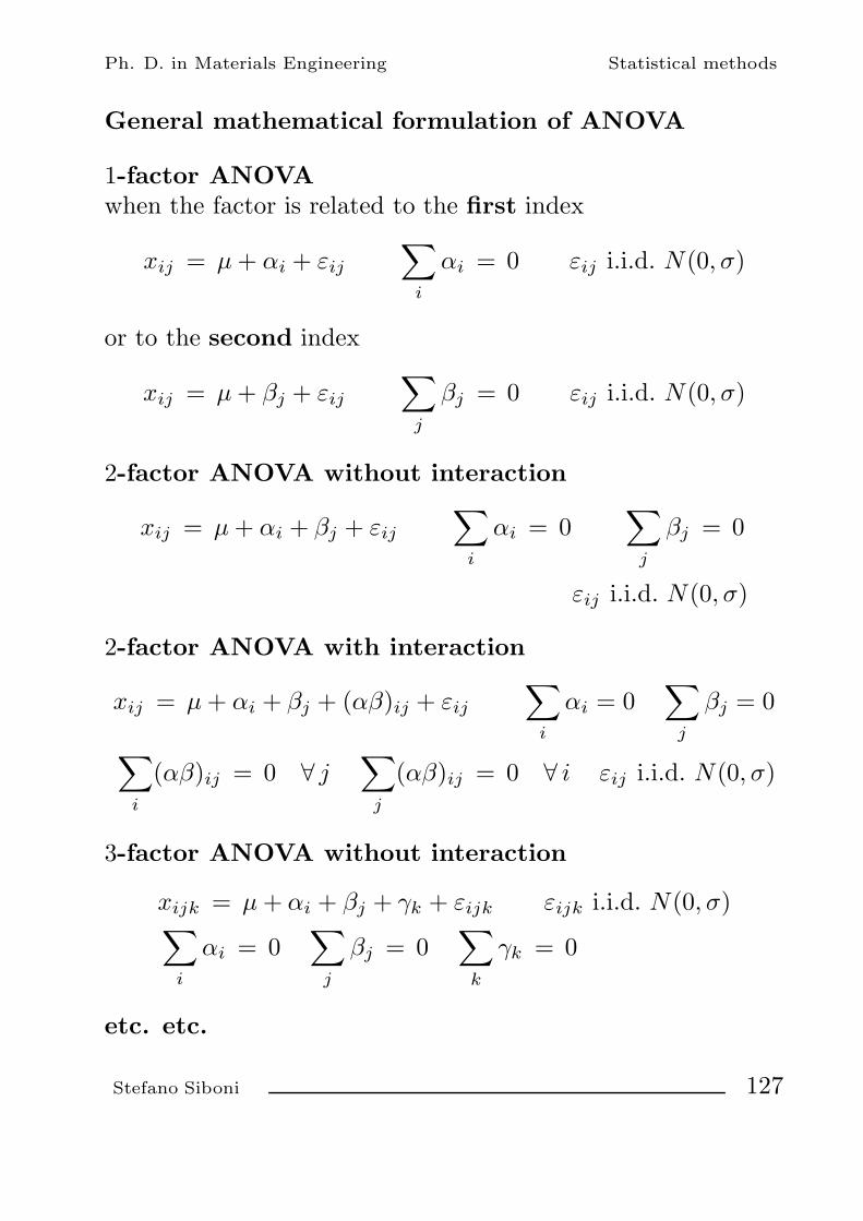
Ph. D. in Materials Engineering Statistical methods
General mathematical formulation of ANOVA
1-factor ANOVAwhen the factor is related to the first index
xij = µ + αi + εij
∑i
αi = 0 εij i.i.d. N (0, σ)
or to the second index
xij = µ + βj + εij
∑j
βj = 0 εij i.i.d. N (0, σ)
2-factor ANOVA without interaction
xij = µ + αi + βj + εij
∑i
αi = 0∑
j
βj = 0
εij i.i.d. N (0, σ)
2-factor ANOVA with interaction
xij = µ + αi + βj + (αβ)ij + εij
∑i
αi = 0∑
j
βj = 0
∑i
(αβ)ij = 0 ∀ j∑
j
(αβ)ij = 0 ∀ i εij i.i.d. N (0, σ)
3-factor ANOVA without interaction
xijk = µ + αi + βj + γk + εijk εijk i.i.d. N (0, σ)∑i
αi = 0∑
j
βj = 0∑
k
γk = 0
etc. etc.
Stefano Siboni 127

Ph. D. in Materials Engineering Statistical methods
5.9.1 1-factor ANOVA
The 1-factor ANOVA makes use of some fundamental defini-tions
Mean of data
x =1rc
r∑i=1
c∑j=1
xij =1rc
∑i,j
xij
Mean of a samplethe mean of the data in a row, i.e. within a sample
xi· =1c
c∑j=1
xij
Residualdifference between the value of a variable and the mean of data
xij − x
Residual “explained” by the factor corresponding toindex ithe part of the residual which can be attributed to the differ-ent means of the various samples, as estimated by the relativesample mean
xi· − x
“Unexplained” residualthe remaining component of the residual, which describes thespread of the data within the sample (i.e. within the rows)
xij − x − (xi· − x) = xij − xi·
Stefano Siboni 128
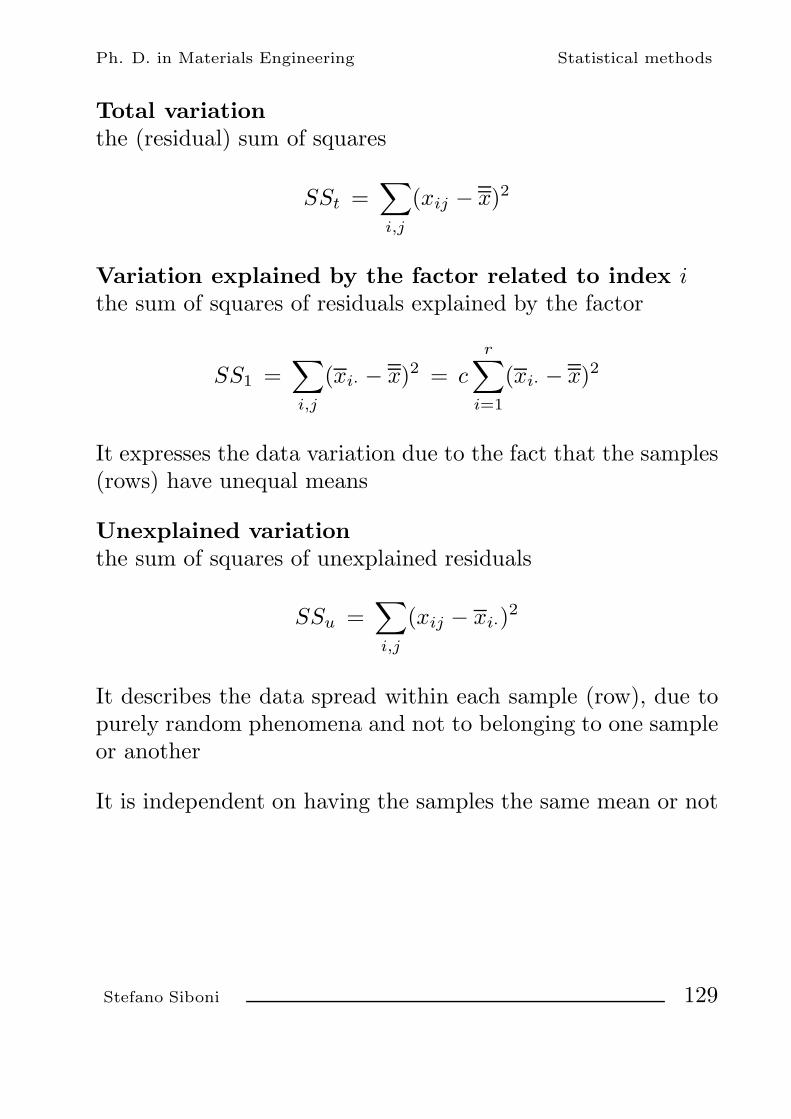
Ph. D. in Materials Engineering Statistical methods
Total variationthe (residual) sum of squares
SSt =∑i,j
(xij − x)2
Variation explained by the factor related to index ithe sum of squares of residuals explained by the factor
SS1 =∑i,j
(xi· − x)2 = c
r∑i=1
(xi· − x)2
It expresses the data variation due to the fact that the samples(rows) have unequal means
Unexplained variationthe sum of squares of unexplained residuals
SSu =∑i,j
(xij − xi·)2
It describes the data spread within each sample (row), due topurely random phenomena and not to belonging to one sampleor another
It is independent on having the samples the same mean or not
Stefano Siboni 129

Ph. D. in Materials Engineering Statistical methods
1-factor ANOVA
Model:
xij = µ + αi + εij i = 1, . . . , r j = 1, . . . , c
with: ∑i
αi = 0
andεij i.i.d. random variables N (0, σ) ∀ i, j
We make the strong assumption that σ is the same for all thevariables
The algebraic identity
∑i,j
(xij − x)2 = total variation SSt
=∑i,j
(xi· − x)2 explained variation SS1
+∑i,j
(xij − xi·)2 unexplained variation SSu
holds independently on the correctness of the model
Stefano Siboni 130

Ph. D. in Materials Engineering Statistical methods
If the model is correct there also holds
1σ2
∑i,j
(xij − x − αi)2 =
=⟨ 1
σ(εij)∣∣∣(I − P1P2)
1σ
(εij)⟩
= X 2rc−1
1σ2
∑i,j
(xi· − x − αi)2 =
=⟨ 1
σ(εij)∣∣∣P2(I − P1)
1σ
(εij)⟩
= X 2r−1
1σ2
∑i,j
(xij − xi·)2 =
=⟨ 1
σ(εij)∣∣∣(I − P2)
1σ
(εij)⟩
= X 2r(c−1)
with X 2r−1 and X 2
r(c−1) stochastically independent
List of symbols:
• (vij) = (v11, v12, . . . , vrc) ∈ Rrc (arbitrary vector of R
rc)
• P1(vij) = (v·j) (operator mean over the 1st index)
• P2(vij) = (vi·) (operator mean over the 2nd index)
• α(vij) = (αvij) ∀α ∈ R, ∀ (vij) ∈ Rrc
• 〈(vij)|(uij)〉 =∑ij
vijuij ∀ (vij), (uij) ∈ Rrc
(usual inner product in Rrc)
Stefano Siboni 131

Ph. D. in Materials Engineering Statistical methods
Fundamental theorem
For any set of data xij the total variation is the sum of thevariation explained by the factor related to i and of the unex-plained one
SSt = SS1 + SSu
If moreover the variables xij are independent and identicallydistributed, with normal distribution of mean µ and varianceσ2, we have that
SSt/σ2 is a X 2 variable with rc − 1 d.o.f.
SS1/σ2 is a X 2 variable with r − 1 d.o.f.
SSu/σ2 is a X 2 variable with rc − r d.o.f.
SS1/σ2 and SSu/σ2 are stochastically independent
Remarks
• we have a balance on the number of d.o.f.
rc − 1 = (r − 1) + (rc − r)
• the (residual) sums of squares divided by the respective num-ber of d.o.f. are defined as variances
SSt/(rc − 1) total variance
SS1/(r − 1) variance explained by the factor considered
SSu/(rc − r) unexplained variance
• the ratio between the explained variance and the unexplainedone
F =SS1
r − 1r(c − 1)
SSu=
r(c − 1)r − 1
SS1
SSu
follows a Fisher distribution with (r − 1, rc − r) d.o.f.
Stefano Siboni 132

Ph. D. in Materials Engineering Statistical methods
Coming back to the model, if the null hypothesis H0 is satisfied
H0 : µi = µ ∀ i = 1, . . . , r
− the ratio F follows a Fisher distribution with (r−1, rc−r)d.o.f.
− the explained variance SS1/(r − 1) is very close to zero
− the unexplained variance — SSu/r(c − 1) — can be as-sumed of the order of σ2
In contrast, if H0 is false (so that at least one of the means µi
turns out to be different from the others) we expect that
1r − 1
SS1>∼ σ2
whereas the unexplained variance is however of the order of σ2
⇓
F is taken as the test variable
and the rejection region of H0 is of the form
F ≥ Fcritical = F[1−α](r−1,r(c−1))
with significance level α(H0 is rejected whenever F turns out to be large enough)
Stefano Siboni 133

Ph. D. in Materials Engineering Statistical methods
Remark
In the conditions assumed for the model — same variance σ2
and means µi for the various samples — it is often importantto determine the confidence intervals of the mean differences
We can apply the following result
Scheffe theoremFor any r-uple of real coefficients (C1, C2, . . . , Cr) with zeromean
r∑i=1
Ci = 0
and for any given α ∈ (0, 1), the inequality∣∣∣∣r∑
i=1
Ci(xi· − µi)∣∣∣∣2
≤ F[α](r−1,rc−r)SSu
r(c − 1)r − 1
c
r∑k=1
C2k
is verified with probability α
We deduce the confidence interval, with confidence level α, ofthe linear combination
∑ri=1 Ciµi
r∑i=1
Cixi· ±√
F[α](r−1,rc−r)
√SSu
r(c − 1)
√√√√r − 1c
r∑k=1
C2k
In particular, for the difference of any two means µi and µh
the confidence interval is
xi· − xh· ±√
F[α](r−1,rc−r)
√SSu
r(c − 1)
√2r − 1
c
again with confidence level α
Stefano Siboni 134

Ph. D. in Materials Engineering Statistical methods
5.9.2 2-factor ANOVA
The set of random variables with two indicesxij i = 1, . . . , r j = 1, . . . , c
describes the measured values of a quantity x concerning amaterial treated by a certain chemical reagent at a given tem-perature
− i identifies the treating chemical reagent
− j specifies the treatment temperature
QuestionHave the chemical reagent or the treatment temperature a sig-nificant effect on the property x of the material?
ModelFor any i = 1, . . . , r and j = 1, . . . , c the random variable xij
is normal with mean µij and variance σ2
RemarkThe mean of the variable xij may depend on both the indicesi and j (on both the chemical reagent and the temperature),while the variance σ2 is the same
Hypothesis to be tested
H0 : µij = µ ∀ i = 1, . . . , r, j = 1, . . . , c (equal means)
H1 : µij = µhj for at least one j and a pair i, h (i = h)orµij = µik for at least one i and a pair j, k (j = k)
Stefano Siboni 135

Ph. D. in Materials Engineering Statistical methods
Definitions
Mean of data
x =1rc
r∑i=1
c∑j=1
xij =1rc
∑i,j
xij
Mean over the index j
xi· =1c
c∑j=1
xij
Mean over the index i
x·j =1r
c∑i=1
xij
Residualxij − x
Residual “explained ” by the factor related to index i
xi· − x
Residual “explained” by the factor related to index j
x·j − x
“Unexplained” residual
xij − x − (xi· − x) − (x·j − x) = xij − xi· − x·j + x
Stefano Siboni 136

Ph. D. in Materials Engineering Statistical methods
Total variation
SSt =∑i,j
(xij − x)2
Variation explainde by the factor related to index i
SS1 =∑i,j
(xi· − x)2 = cr∑
i=1
(xi· − x)2
Variation explained by the factor related to index j
SS2 =∑i,j
(x·j − x)2 = rc∑
j=1
(x·j − x)2
Unexplained variation
SSu =∑i,j
(xij − xi· − x·j + x)2
Stefano Siboni 137

Ph. D. in Materials Engineering Statistical methods
5.9.3 2-factor ANOVA without interaction
Model:
xij = µ + αi + βj + εij i = 1, . . . , r j = 1, . . . , c
with: ∑i
αi = 0∑
j
βj = 0
andεij i.i.d. random variables N (0, σ) ∀ i, j
σ is assumed to be the same for all the variables!
The algebraic identity
∑i,j
(xij − x)2 total variation SSt
=∑i,j
(xi· − x)2 variation explained by the 1st factor, SS1
+∑i,j
(x·j − x)2 variation explained by the 2nd factor, SS2
+∑i,j
(xij − x·j − xi· + x)2 unexplained variation SSu
is independent on the correctness of the model
Stefano Siboni 138
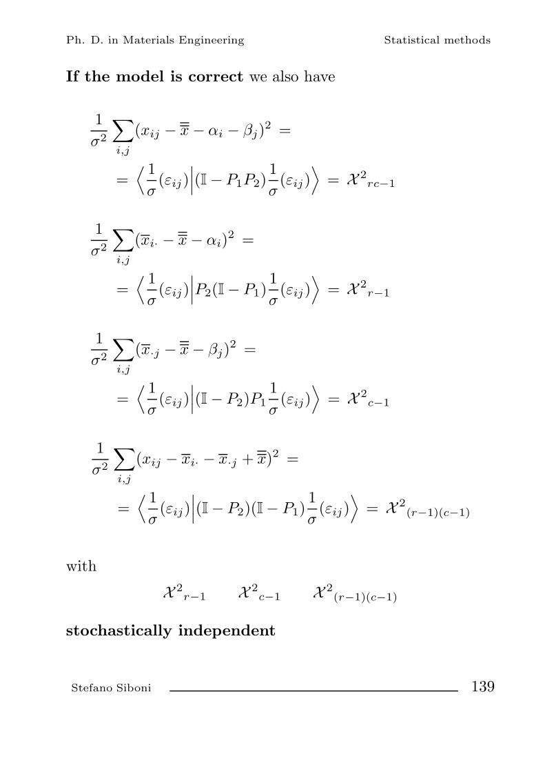
Ph. D. in Materials Engineering Statistical methods
If the model is correct we also have
1σ2
∑i,j
(xij − x − αi − βj)2 =
=⟨ 1
σ(εij)∣∣∣(I − P1P2)
1σ
(εij)⟩
= X 2rc−1
1σ2
∑i,j
(xi· − x − αi)2 =
=⟨ 1
σ(εij)∣∣∣P2(I − P1)
1σ
(εij)⟩
= X 2r−1
1σ2
∑i,j
(x·j − x − βj)2 =
=⟨ 1
σ(εij)∣∣∣(I − P2)P1
1σ
(εij)⟩
= X 2c−1
1σ2
∑i,j
(xij − xi· − x·j + x)2 =
=⟨ 1
σ(εij)∣∣∣(I − P2)(I − P1)
1σ
(εij)⟩
= X 2(r−1)(c−1)
with
X 2r−1 X 2
c−1 X 2(r−1)(c−1)
stochastically independent
Stefano Siboni 139

Ph. D. in Materials Engineering Statistical methods
Fundamental theorem
For any set xij the total variation coincides with the sum of
− the variation explained by the factor related to i− the variation explained by the factor associated to j− the unexplained variation
SSt = SS1 + SS2 + SSu
If moreover the variables xij are i.i.d. normal of mean µ andvariance σ2, we have that
SSt/σ2 is a X 2 variable with rc − 1 d.o.f.
SS1/σ2 is a X 2 variable with r − 1 d.o.f.
SS2/σ2 is a X 2 variable with c − 1 d.o.f.
SSu/σ2 is a X 2 variable with (r − 1)(c − 1) d.o.f.
SS1/σ2, SS2/σ2 and SSu/σ2 are stochastically independent
Stefano Siboni 140
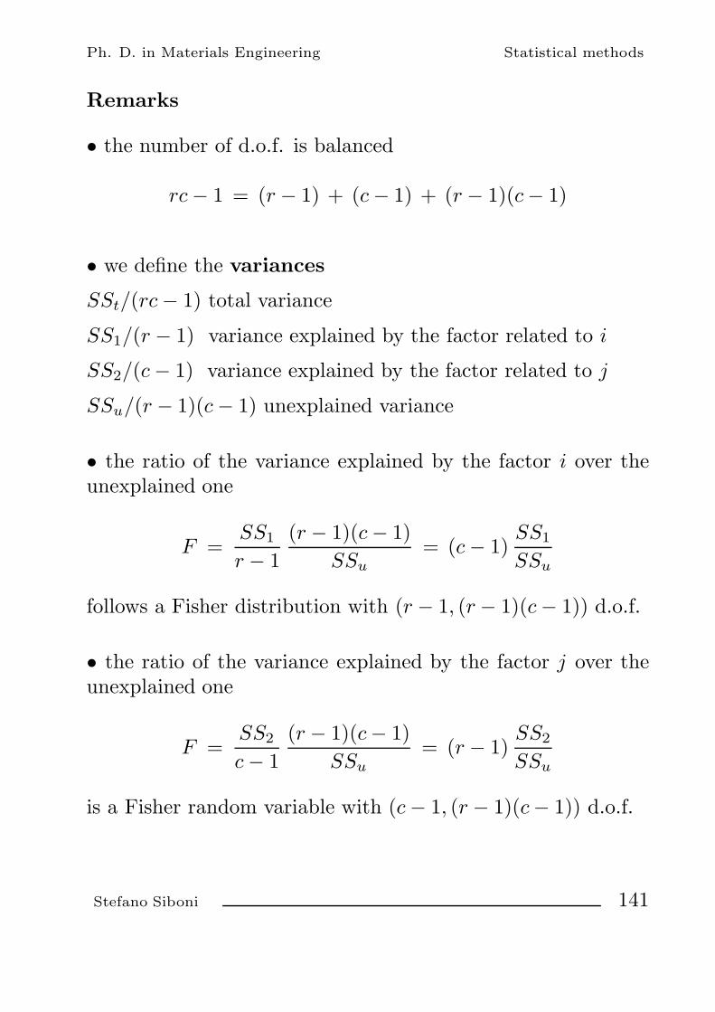
Ph. D. in Materials Engineering Statistical methods
Remarks
• the number of d.o.f. is balanced
rc − 1 = (r − 1) + (c − 1) + (r − 1)(c − 1)
• we define the variances
SSt/(rc − 1) total variance
SS1/(r − 1) variance explained by the factor related to i
SS2/(c − 1) variance explained by the factor related to j
SSu/(r − 1)(c − 1) unexplained variance
• the ratio of the variance explained by the factor i over theunexplained one
F =SS1
r − 1(r − 1)(c − 1)
SSu= (c − 1)
SS1
SSu
follows a Fisher distribution with (r − 1, (r − 1)(c − 1)) d.o.f.
• the ratio of the variance explained by the factor j over theunexplained one
F =SS2
c − 1(r − 1)(c − 1)
SSu= (r − 1)
SS2
SSu
is a Fisher random variable with (c − 1, (r − 1)(c − 1)) d.o.f.
Stefano Siboni 141
Ph. D. in Materials Engineering Statistical methods
Test for the difference of the mean over the index i
Test variable
F =SS1
r − 1(r − 1)(c − 1)
SSu= (c − 1)
SS1
SSu
If the mean µij do not depend appreciably on the index i, thereholds
SS1
r − 1 SSu
(r − 1)(c − 1) σ2 ⇐⇒ F small
whereas in the opposite case we expect that
SS1
r − 1>∼
SSu
(r − 1)(c − 1) σ2 ⇐⇒ F large
We define then a critical value of F
Fcritical = F[1−α](r−1,(r−1)(c−1))
and an acceptance region of H0 — means independent on theindex i —
F ≤ F[1−α](r−1,(r−1)(c−1))
along with a corresponding rejection region — means µij
appreciably dependent on the index i —
F > F[1−α](r−1,(r−1)(c−1))
both with given significance level α ∈ (0, 1)
Stefano Siboni 142

Ph. D. in Materials Engineering Statistical methods
Test for the difference of the means over the index j
Test variable
F =SS2
c − 1(r − 1)(c − 1)
SSu= (r − 1)
SS2
SSu
If the means µij do not depend appreciably on the index j wehave
SS2
c − 1 SSu
(r − 1)(c − 1) σ2 ⇐⇒ F small
while in the opposite case it seems reasonable to assume that
SS2
c − 1>∼
SSu
(r − 1)(c − 1) σ2 ⇐⇒ F large
We define then a critical value of F
Fcritical = F[1−α](c−1,(r−1)(c−1))
and an acceptante region of H0 — means independent on theindex j —
F ≤ F[1−α](c−1,(r−1)(c−1))
along with a corresponding rejection region — means µij
appreciably dependent on the index j —
F > F[1−α](c−1,(r−1)(c−1))
both with given significance level α ∈ (0, 1)
Stefano Siboni 143

Ph. D. in Materials Engineering Statistical methods
5.9.4 2-factor ANOVA with interaction
Model:
xijk = µ + αi + βj + αβij + εijk
i = 1, . . . , r j = 1, . . . , c k = 1, . . . , s
with: ∑i
αi = 0∑
j
βj = 0
∑i
αβij = 0 ∀ j∑
j
αβij = 0 ∀ i
andεijk i.i.d. random variables N (0, σ) ∀ i, j, k
The algebraic identity∑ijk
(xijk − x)2 total variation SSt
=∑ijk
(xi·· − x)2 var.on explained by the 1st factor, SS1
+∑ijk
(x·j· − x)2 var.on explained by the 2nd factor, SS2
+∑ijk
(xij· − x·j· − xi·· + x)2 var.on explained by the interactionbetween the factors 1 and 2, S12
+∑ijk
(xijk − xij·)2 unexplained variation SSu
holds also when the model is incorrect
Stefano Siboni 144

Ph. D. in Materials Engineering Statistical methods
Moreover, if the model is correct we have that
1σ2
∑ijk
(xijk − x − αi − βj − αβij)2 =
=⟨ 1
σ(εijk)
∣∣∣(I − P3P2P1)1σ
(εijk)⟩
= X 2rcs−1
1σ2
∑ijk
(xi·· − x − αi)2 =
=⟨ 1
σ(εijk)
∣∣∣P3P2(I − P1)1σ
(εijk)⟩
= X 2r−1
1σ2
∑ijk
(x·j· − x − βj)2 =
=⟨ 1
σ(εijk)
∣∣∣P3(I − P2)P11σ
(εijk)⟩
= X 2c−1
1σ2
∑ijk
(xij· − x·j· − xi·· + x − αβij)2 =
=⟨ 1
σ(εijk)
∣∣∣P3(I − P2)(I − P1)1σ
(εijk)⟩
= X 2(r−1)(c−1)
1σ2
∑ijk
(xijk − xij·)2 =
=⟨ 1
σ(εijk)
∣∣∣(I − P3)1σ
(εijk)⟩
= X 2rc(s−1)
with
X 2r−1 X 2
c−1 X 2(r−1)(c−1) X 2
rc(s−1)
stochastically independent
Stefano Siboni 145

Ph. D. in Materials Engineering Statistical methods
5.10 Sign test for the median of a population
Non-parametric test: it does not require any hypothesisabout the form of the probability distribution of the population
Let us consider a discrete or continuous random variable x ofarbitrary distribution p(x)
Hypothesis to be tested:
H0: the median of the distribution is m
H1: the median of the distribution is different from m
If the median of the population holds m, then:
x − m > 0 with probability 1/2
x − m ≤ 0 with probability 1/2
otherwise we will have a larger probability of obtaining positiveor negative residuals
Test variableFor a set x1, x2, . . . , xn of outcomes of x we pose
si =
1 if xi − m > 00 if xi − m ≤ 0
∀ i = 1, . . . , n
and introduce as a test variable the number of positive differ-ences with respect to the median
z =n∑
i=1
si
Stefano Siboni 146

Ph. D. in Materials Engineering Statistical methods
Rejection region
We are led to reject the hypothesis H0 whenever the numberof positive differences with respect to the median turns out tobe too large or too small
The rejection region will be two-sided and symmetrical
z ≤ zmin ∪ z ≥ zmax
If the hypothesis H0 holds true, the test variable z follows abinomial distribution with p = 1/2
pn(z) =(n
z
) 12n
∀ z = 0, 1, . . . , n
For a given significance level α of the test, the bounds zmin andzmax of the rejection region are therefore defined by
zmin∑z=0
(n
z
) 12n
=α
2
n∑z=zmax
(n
z
) 12n
=α
2
Stefano Siboni 147

Ph. D. in Materials Engineering Statistical methods
5.11 Sign test to check if two paired samplesbelong to the same population
The sign test is very useful to check whether two paired samplesare drawn from the same statistical population,
i.e. if two paired samples follow the same probability distribu-tion
The test relies on the remark that for any two independentcontinuous random variables x and y with the same probabilitydistribution p(x) — or p(y) — the difference RV
z = x − y
follows an even probability distribution
pz(z) = pz(−z) ∀ z ∈ R
no matter the common distribution p(x) is.
We have indeed
1 =∫R
dy
∫R
dx p(x) p(y) =∫R
dy
∫R
dz p(y + z) p(y) =
=∫R
dz
∫R
dy p(y + z) p(y)
so that the probability distribution of z is
pz(z) =∫R
p(y + z) p(y) dy ∀ z ∈ R .
Stefano Siboni 148

Ph. D. in Materials Engineering Statistical methods
Consequently,
pz(−z) =∫R
p(y − z) p(y) dy
and by the change of variable y = ξ + z the integral becomes
pz(−z) =∫R
p(ξ) p(ξ + z) dξ =∫R
p(ξ + z) p(ξ) dξ = pz(z) .
Positive and (null or) negative differences have then the sameprobability to occur:
p(z > 0) =12
p(z ≤ 0) =12
.
Thus we can test the null hypothesis
H0 : the two samples are drawn from the same population
versus the alternative hypothesis
H1 : the two samples are drawn from unlike populations
by using as a test variable the number z of the positivedifferences detected on the various data pairs of the sample
H0 will be accepted if z is close to half the number of datapairs of the sample, while H1 will be preferred whenever z issufficiently low or too large (two-sided critical region)
Stefano Siboni 149

Ph. D. in Materials Engineering Statistical methods
The rejection region takes then the two-sided form
z ≤ zmin ∪ z ≥ zmaxIf H0 holds true, the variable z obeys a binomial distributionwith p = 1/2 and the probability that z takes a value withinthe critical region must be identified with the probability α ofmaking a type I error
At the significance level α, the limits zmin and zmax of thecritical region are thus defined by
zmin∑z=0
(n
z
) 12n
=α
2
n∑z=zmax
(n
z
) 12n
=α
2
Example: Sign testA company states that by adding an additive of own manu-facture to the reservoir of a gasoline car the efficiency of theengine increases. To check this statement 16 cars are chosenand the mean distance that they cover by a litre of fuel, withand without additive, is measured (in Km).
additive no additive additive no additive17.35 15.70 13.65 13.1014.15 13.60 16.05 15.709.80 10.20 14.80 14.40
12.55 12.30 11.20 11.557.85 7.45 12.65 12.00
12.25 11.15 14.05 13.6514.35 13.40 12.15 11.4511.75 12.05 11.95 12.40
Stefano Siboni 150

Ph. D. in Materials Engineering Statistical methods
Assuming that the drive conditions are the same, check if thereis any difference in the performances of the engines due to theuse of the additive, with a significance level of 5% and 1%.
SolutionWe must test the null hypothesis H0 that no difference of per-formances occurs between the cars fed with additivated fueland the same vehicles filled up with normal gasoline, versusthe alternative hypothesis H1 that the cars filled up with ad-ditivated fuel have better performances.
The hypothesis H0 is rejected in favour of H1 only if the numberof positive differences is sufficiently large: the test is one-sided.
The distances per litre covered by the additivated and the non-additivated cars show 12 positive differences and 4 nega-tive differences.
If H0 is correct, the probability of having at least 12 positivesigns out of 16 differences writes
16∑z=12
(16z
) 1216
=
=[(16
12
)+(16
13
)+(16
14
)+(16
15
)+(16
16
)] 1216
= 0.0384
so that the observed number 12 of positive signs certainly be-longs to the rejection region of H0 if the significance level istaken at 5%. In contrast, if α = 1% the number z = 12 ofpositive differences does not fall within the critical region ofH0, which then cannot be rejected.
Stefano Siboni 151

Ph. D. in Materials Engineering Statistical methods
5.12 Detection of outliers by Chauvenet criterion
Let a small sample of data x1, x2, . . . xn be given
Assume that data are drawn from a normal population
Suppose that a datum xk is very far from the sample mean x
Problem: does xk actually belong to the normal population,or is it an “intruder”?
A possible strategy (Chauvenet criterion):
Let us pose
z =|xk − x|
s |xk − µ|
σ
where µ and σ are replaced with the sample estimate x and srespectively (with fingers crossed!)
z is the distance of xk from the sample mean x in units of s
or, approximately, from the mean µ in units of σ
Stefano Siboni 152

Ph. D. in Materials Engineering Statistical methods
The probability p(z) that a normal datum xk is at a distance≥ z from the mean, in units of σ, is represented by the shadedarea in the following graph of the N (µ, σ) distribution
The probability p(z) can be expressed as
p(z) = 1 −µ+zσ∫
µ−zσ
1√2πσ
e−(x−µ)2/2σ2dx
or, after some change of variables, in the equivalent forms
p(z) = 1 − 2√2π
z∫0
e−ξ2/2dξ = 1 − erf( z√
2
)
where erf denotes the error function:
erf(x) =2√π
x∫0
e−t2dt
Stefano Siboni 153

Ph. D. in Materials Engineering Statistical methods
The mean number of data at a distance ≥ z from µ in σ unitsout of n measurements is
n p(z)
Let us choose z so that the mean number of data as before issignificantly smaller than 1. Typically we require that:
n p(z) =12i.e.
1 − erf( z√
2
)=
12n
(1)
With the previous z, if|xk − x|
s≥ z
it is quite unlikely that xk belongs to the normal population
In such a case, the datum should be rejected as meaningless
The graph shows the critical value z versus the number n ofdata
Stefano Siboni 154

Ph. D. in Materials Engineering Statistical methods
The following table collects the critical values z versus thenumber n of data, according to the previous equation (1):
n critical z n critical z1 0.674489750 27 2.3550840092 1.150349380 28 2.3685670593 1.382994127 29 2.3815194704 1.534120544 30 2.3939798005 1.644853627 40 2.4977054746 1.731664396 50 2.5758293047 1.802743091 60 2.6382572738 1.862731867 70 2.6901095279 1.914505825 80 2.73436878710 1.959963985 90 2.77292129511 2.000423569 100 2.80703376812 2.036834132 150 2.93519946913 2.069901831 200 3.02334144014 2.100165493 250 3.09023230615 2.128045234 300 3.14398028716 2.153874694 350 3.18881525917 2.177923069 400 3.22721842618 2.200410581 450 3.26076748819 2.221519588 500 3.29052673120 2.241402728 550 3.31724736221 2.260188991 600 3.34147895622 2.277988333 650 3.36363545623 2.294895209 700 3.38403625224 2.310991338 800 3.42052670125 2.326347874 900 3.45243293726 2.341027138 1000 3.480756404
Stefano Siboni 155

Ph. D. in Materials Engineering Statistical methods
Example: Chauvenet criterion
Repeated measurements of a length x have provided the fol-lowing results (expressed in mm):
46 , 48 , 44 , 38 , 45 , 47 , 58 , 44 , 45 , 43
and can be assumed to be drawn from a normal population.By applying Chauvenet criterion, we want to check whetherthe anomalous result (outlier) xsus = 58 must be rejected.
SolutionThe sample mean and standard deviation are given by
x =110
10∑i=1
xi = 45.8 s =
√√√√19
10∑i=1
(xi − x)2 = 5.1
The distance of the suspect value from the mean, in units of s,holds
xsus − x
s=
58 − 45.85.1
= 2.4
The probability that a measurement falls at a distance largerthan 2.4 standard deviations from the mean can be calculatedfrom the Table of the cumulative distribution function of thestandard normal distribution:
P (|xsus − x| ≥ 2.4s) = 1 − P (|xsus − x| < 2.4s) == 1 − 2 · P (x ≤ xsus < x + 2.4s) == 1 − 2 · 0.49180 = 0.0164
Out of 10 measurements we typically expect 10 · 0.0164 = 0.164“bad” results, at a distance larger than 2.4s from the mean.Since 0.164 < 1/2 Chauvenet criterion suggests that theoutlier xsus should be rejected.
Stefano Siboni 156
Ph. D. in Materials Engineering Statistical methods
6. PAIRS OF RANDOM VARIABLES6.1 Linear correlation coefficient (Pearson r)
Let (x, y) be a pair of random variables
Problem: are they stochastically dependent or independent?
The limit case of stochastic dependence is that whereone variable is a function of the other
y=f(x)
The most interesting case is the linear one, when we assumey = ax + b, with given constants a and b (a = 0)
The joint probability distribution of (x, y)can be formally written as
p(x, y) = p(x) δ(ax + b − y)in terms of the generalized function Dirac delta δ
Stefano Siboni 157

Ph. D. in Materials Engineering Statistical methods
Means, variances and covariance of (x, y) take then the form:
µx =∫R2
p(x) δ(ax + b − y)x dydx =∫R
p(x)x dx
µy =∫R2
p(x) δ(ax + b − y)y dydx = aµx + b
var(x) =∫R2
p(x) δ(ax+b−y)(x−µx)2dydx =∫R
p(x)(x−µx)2dx
var(y) =∫R2
p(x) δ(ax + b − y)(y − µy)2dydx =
=∫R
p(x)(ax − aµx)2dx = a2
∫R
p(x)(x − µx)2dx
cov(x, y) =∫R2
p(x) δ(ax + b − y)(x − µx)(y − µy)dydx =
=∫R
p(x)(x − µx)(ax − aµx)dx = a
∫R
p(x)(x − µx)2dx
so that the correlation becomes
corr(x, y) =cov(x, y)√
var(x)√
var(y)=
a
|a| =+1 if a > 0−1 if a < 0
If (x, y) are independent we have instead corr(x, y) = 0
Stefano Siboni 158

Ph. D. in Materials Engineering Statistical methods
Whenever y is a nonlinear function f(x) of the RV x, thecorrelation between x and y
corr(x, y) =
∫R
p(x)(x − µx)[f(x) − µy]dx
√√√√∫R
p(x)(x − µx)2dx
√√√√∫R
p(x)[f(x) − µy]2dx
withµy =
∫R
p(x)f(x) dx
has no particular meaning
Nevertheless, the values of corr(x, y) can be considered as anindication of:
− direct linear dependence (a > 0), if close to +1;
− inverse linear dependence (a < 0), when close to −1;
− stochastic independence, if close to 0
Stefano Siboni 159

Ph. D. in Materials Engineering Statistical methods
Let (xi, yi) ∈ R2, i = 1, . . . , n be a sample of the pair of random
variables (x, y), with sample means x and y respectively
The correlation is then estimated by using the sample, bymeans of the (Pearson) linear correlation coefficient
r =
n∑i=1
(xi − x)(yi − y)
√√√√ n∑i=1
(xi − x)2
√√√√ n∑i=1
(yi − y)2
Actually, from Cauchy-Schwarz inequality
n∑i=1
aibi ≤
√√√√ n∑i=1
a2i
√√√√ n∑i=1
b2i ∀ai, bi ∈ R i = 1, . . . , n
it follows that the condition r = +1 or r = −1 is equivalentto have all the pairs (xi, yi) of the sample arranged along thesame straight line, of positive or negative slope respectively
Stefano Siboni 160

Ph. D. in Materials Engineering Statistical methods
6.2 Statistics of the linear correlation coefficientOnce the stochastic dependence of the random variables (x, y)has been established, the linear correlation coefficient expressesconventionally the “intensity” of such a dependence
But, generally speaking, the coefficient r is not a good indica-tor to test the stochastic dependence or independence of thevariables (x, y)
Indeed, even if the null hypothesisH0 : the variables x and y are independent
holds true, the probability distribution of r is not determined,since those of x and y are unknown
⇓
It is impossible to devise a test in order to check the hypothesisH0, with an appropriate significance level
It is necessary to refer to some noticeable cases, forwhich the distribution of r can be at least partially determined
Stefano Siboni 161

Ph. D. in Materials Engineering Statistical methods
6.2.1 Independent random variables (x, y)For a pair of independent random variables (x, y), whoseprobability distributions have a sufficiently large number ofconvergent moments, if n is large enough (n > 20)
⇓
r follows approximately a normal distributionwith zero average and variance 1/n
⇓
The rejection region of H0 will be the union of intervals
|r| ≥ η = r < −η ∪ r > η
where η > 0 is determined by the equation
α
2=√
n
2π
∫ +∞
η
e−z2n/2dz =12erfc(η
√n
2
)
and erfc denotes the complementary error function
erfc(x) = 1 − erf(x) = 1 − 2√π
∫ x
0
e−ξ2dξ =
2√π
∫ ∞
x
e−ξ2dξ
while α is the probability of a type I error
Stefano Siboni 162

Ph. D. in Materials Engineering Statistical methods
6.2.2 Normal random variables (x, y)For normal variables (x, y), with distribution
p(x, y) =12π
√a11a22 − a2
12 e−12 (a11x2−2a12xy+a22y2)
a11a22 − a212 > 0 a11 + a22 > 0
and hence correlation
ρ = corr(x, y) =a12√
a11√
a22∈ (−1, 1)
the theoretical frequency distribution of r depends on ρ and onthe number n of datapoints.
Defined for r ∈ (−1, 1), such a distribution can be written:
pρ,n(r) =2n−3
π(n − 3)!(1 − ρ2)(n−1)/2(1 − r2)(n−4)/2aρ,n(r)
with
aρ,n(r) =∞∑
s=0
Γ2(n + s − 1
2
) (2ρr)s
s!
The distribution is just too complex to be used directly
Typically an approximation is used which holds true for largesamples (n ≥ 10)
Or, alternatively, we refer to the case ρ = 0 of uncorrelated⇐⇒ independent variables (what we are usually interested in)
Stefano Siboni 163

Ph. D. in Materials Engineering Statistical methods
6.2.2.1 Approximation for large n of normal variablesFisher transformation
For n large enough (n ≥ 10), the Fisher z variable:
z = arctanh r =12
ln1 + r
1 − r
follows approximately a normal distributionof mean
z =12
[ln
1 + ρ
1 − ρ+
ρ
n − 1
]and standard deviation
σ(z) 1√n − 3
The Fisher transformation is implemented in Excel by the func-tion FISHER
6.2.2.2 Independent (or uncorrelated) normal variables
For ρ = 0 the probability distribution of r reduces to:
p0,n(r) =Γ[(n − 1)/2]√πΓ[(n − 2)/2]
(1 − r2)(n−4)/2
in such a way that the random variable:
t =√
n − 2r√
1 − r2
follows a Student’s distribution with n − 2 d.o.f.
Stefano Siboni 164

Ph. D. in Materials Engineering Statistical methods
In the case of normal variables (x, y) it is then possible totest the hypothesis
H0 : x and y are independent variables
which will be regarded as acceptable when the test variable
t =√
n − 2r√
1 − r2
is close enough to 0 (and also r almost vanishes)
The null hypothesis H0 will be rejected if in contrast t (andthus r) is significantly different from zero
We deduce a typical two-sided test, with a rejection regiondefined by
t ≤ t[ α2 ](n−2)
∪t ≥ t[1−α
2 ](n−2)
i.e.
t ≤ −t[1−α2 ](n−2)
∪t ≥ t[1−α
2 ](n−2)
with significance level α
Stefano Siboni 165

Ph. D. in Materials Engineering Statistical methods
Example: Linear correlation coefficient (Pearson r)Let us consider the following table of data, concerning somerepeated measurements of two quantities x and y (in arbitraryunits), gathered in the same experimental conditions. Thesample is assumed to be normal.
i xi yi
1 1.8 1.12 3.2 1.63 4.3 1.14 5.9 3.55 8.1 3.86 9.9 6.27 11.4 5.68 12.1 4.09 13.5 7.5
10 17.9 7.1
Use Pearson’s linear correlation coefficient to check whetherthe quantities x and y can be considered stochastically inde-pendent, with a significance level of 5% and 1%.
SolutionThe sample means of the quantities are given by
x =110
10∑i=1
xi = 8.8100 y =110
10∑i=1
yi = 4.1500
and allow us to reckon the following sums of residual products
SSxy =10∑
i=1
(xi − x)(yi − y) = 99.6050
Stefano Siboni 166
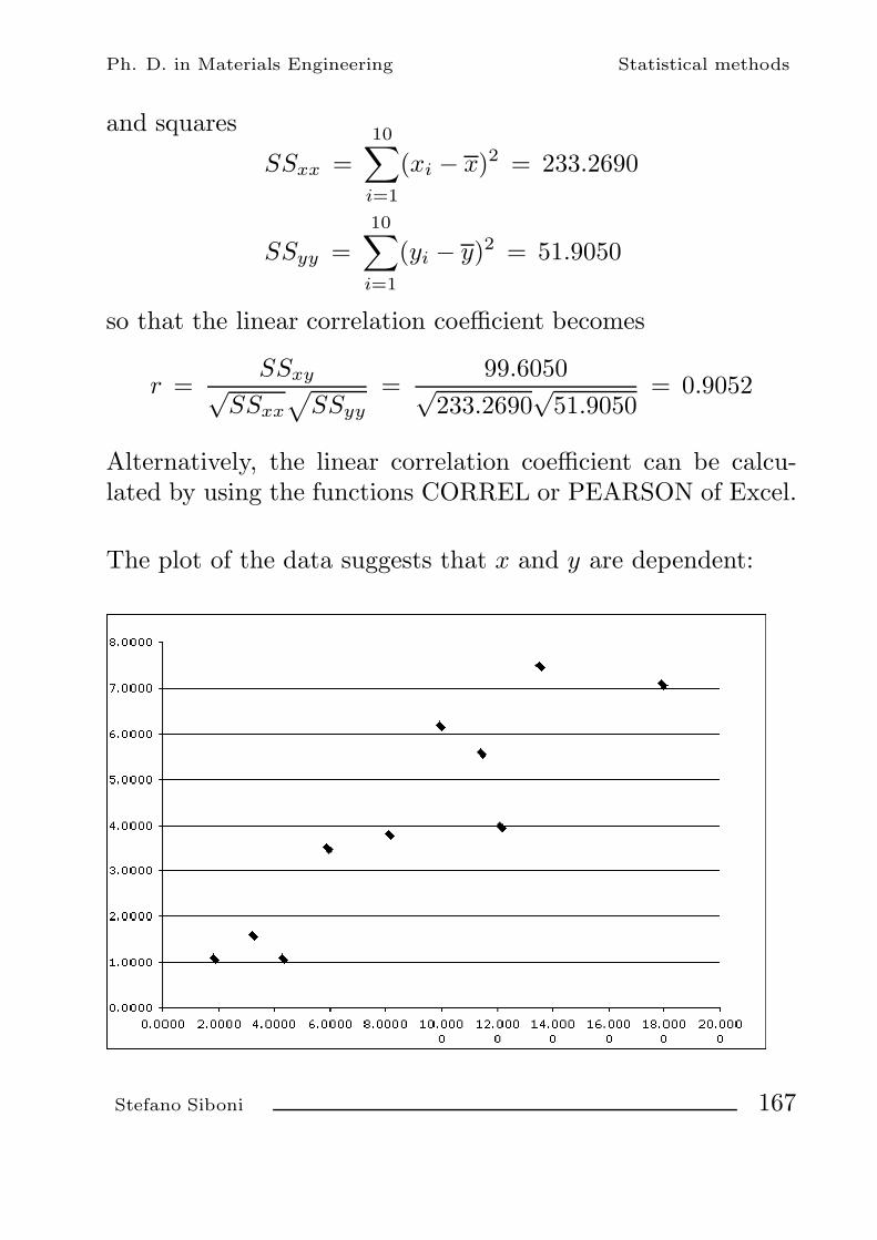
Ph. D. in Materials Engineering Statistical methods
and squares
SSxx =10∑
i=1
(xi − x)2 = 233.2690
SSyy =10∑
i=1
(yi − y)2 = 51.9050
so that the linear correlation coefficient becomes
r =SSxy√
SSxx
√SSyy
=99.6050√
233.2690√
51.9050= 0.9052
Alternatively, the linear correlation coefficient can be calcu-lated by using the functions CORREL or PEARSON of Excel.
The plot of the data suggests that x and y are dependent:
Stefano Siboni 167

Ph. D. in Materials Engineering Statistical methods
As x and y can be assumed to be normal, we can test thenull hypothesis
H0 : x and y are stocastically independent
versus the alternative hypothesis
H1 : x and y are stochastically dependent
by means of the RV
t =√
n − 2r√
1 − r2
which, for H0 true, follows a Student distribution with n − 2d.o.f. In the present case we get
t =√
10 − 20.9052√
1 − 0.90522= 6.0247
The critical region takes the form
|t| > t[1−α2 ](n−2) = t[0.975](8) = 2.306
for a significance level α = 5%, and the form
|t| > t[1−α2 ](n−2) = t[0.995](8) = 3.355
when the required significance level is α = 1%.
In both cases H0 must be rejected!
Stefano Siboni 168

Ph. D. in Materials Engineering Statistical methods
6.3 Remark
We have considered the circumstance that the linear correlationcoefficient r is calculated for a small sample of two randomvariables (x, y)
In many cases, however, the coefficient is calculated in a com-pletely different situation, when the pairs (xi, yi):
- cannot be regarded as individuals drawn from the samestatistical population
- can be grouped into some subsets, each of which belong-ing to a proper statistical population
Example: experiments directed to detect the variations of aquantity y due to the variations of another quantity x
The data (xi, yi) cannot be regarded as the outcomes of onepair of random variables
⇓
r does not follow a known probability distribution and can-not be applied to test the stochastic dependence or indepen-dence of the quantities x and y
r provides an indication on the degree of alignment of data(xi, yi), but it offers no statistical information about the sig-nificance of the suggested linear dependence
Such a significance must be verified in a different way: problemof the linear regression and of the goodness of fit
Stefano Siboni 169

Ph. D. in Materials Engineering Statistical methods
7. DATA MODELING
7.1 General setup of the problem
Measurements
⇓
Data of the form (xi, yi), i = 1, . . . , n
⇓
Synthesis of data into a “model”
“Model” is a mathematical functionwhich relates the observed quantities among themselvesand depends on suitable parameters to be “adjusted”
The procedure to adjust the value of the parameters is known as“fitting”
As a rule, the fitting procedure consists:
(i) in the definition of a suitable objective function (or meritfunction), which describes the agreement between data andmodel for a given choice of the parameters;
(ii) in the subsequent calculation of the model parameters bythe optimization of the merit function (best fit)
Stefano Siboni 170

Ph. D. in Materials Engineering Statistical methods
We assume that
good agreementmodel/data ⇐⇒
small valuesof the merit function
so that
best fit ⇐⇒search for the minimumof the merit function
It is not, however, a simple optimization problem (search forthe best-fit values of the parameters):
• data are typically affected by errors and must be regardedas the outcomes of appropriate RVs;
• the best-fit parameters of the model are then affectedby an error and must be assumed in turn as RVs;
• errors and, eventually, the probability distribution ofthe best-fit parameters must be determined;
- appropriate tests are required in order to check whetherthe model is or is not adequate to describe data(goodness of fit)
Stefano Siboni 171

Ph. D. in Materials Engineering Statistical methods
Merit function
The choice of the merit function often relies on the so-calledmaximum likelihood method
• We assume that the parameters are determined in such away that the data actually measured constitute an event ofmaximum probability: the set of measured data is the mostprobable one, whose occurrence is most likely
• Assumed that the variables xi have negligible variance andcan be considered almost certain, and that the yi are indepen-dent normal variables of variance σ2
i , the maximum likelihoodleads to the chi-square method
• Whenever, in the same hypotheses, the variances of the vari-ables yi can be considered equal, the maximum likelihood ap-proach reduces to a least-squares fitting
• The maximum likelihood method can be applied also in thecase of non-normal variables
It may happen that the probability distributions of yi can-not be considered normal because of outcomes noticeablydifferent from the means, whose occurrence would be al-most impossible for normal variables (outliers, outcomeswhich differ from the mean for more than 3 standard de-viations )
In such a case, the merit functions obtained by the maximumlikelihood approach characterize the so-called “robust” fit-ting methods
Stefano Siboni 172

Ph. D. in Materials Engineering Statistical methods
Maximum Likelihood and Chi-square
Probability of obtaining the pairs of data (xi, yi), i = 1, . . . , n
P (x1, y1, . . . , xn, yn) ∼n∏
i=1
e− 1
2σ2i
[yi − R(xi)]2=
= e
−12
n∑i=1
1σ2
i
[yi − R(xi)]2
in the assumption of variables xi completely certain and yi
independent normal with mean R(xi) and variance σ2i
The Maximum Likelihood method consists in requiring that
P (x1, y1, . . . , xn, yn) be maximum
or, equivalently, that
n∑i=1
1σ2
i
[yi − R(xi)]2 be minimum
i.e. that the chi-square of data yi with respect to the regressionfunction R(x) be minimum — chi-square method
Stefano Siboni 173

Ph. D. in Materials Engineering Statistical methods
7.2 Linear regression by the chi-square method(chi-square fitting)
Let (xi, yi) ∈ R
2 , 1 ≤ i ≤ n
be a set of data satisfying the following conditions:
(i) for each i = 1, . . . , n the datum yi is the outcome of anormal RV of known variance σ2
i . The mean value of thisvariable is a priori unknown, but it is assumed to dependexclusively on the abscissa xi — of which it will be a func-tion;
(ii) the set of data is described by the mathematical model
ζi =p∑
j=1
αjφj(xi) + εi , 1 ≤ i ≤ n , (2)
in which φj : R−−−−→R, 1 ≤ j ≤ p, are p < n givenfunctions and αj , 1 ≤ j ≤ p, some constant parameters tobe conveniently estimated, while the εi’s constitute a setof n independent normal variables of vanishing mean andvariance σ2
i
E(εi) = 0 E(εiεk) = δikσ2k 1 ≤ i, k ≤ n .
The value yi must be regarded as an outcome of the RVζi, for each i.
Stefano Siboni 174

Ph. D. in Materials Engineering Statistical methods
We define linear regression of the data set, by the chi-squaremethod (chi-square fitting), the expression
R(x) =p∑
j=1
ajφj(x) , x ∈ R ,
where the aj ’s are the estimates of the parameters αj obtainedby means of the sample (xi, yi) , 1 ≤ i ≤ n by minimizingthe quadratic functional L : R
p −−−−→R defined by
L(α1, . . . , αp) =n∑
i=1
1σ2
i
[−yi +
p∑j=1
αjφj(xi)]2
(3)
If the variances σ2i of the RVs εi are all equal, their common
value can be ignored in the minimization of the functional (3),which reduces therefore to
L(α1, . . . , αp) =n∑
i=1
[−yi +
p∑j=1
αjφj(xi)]2
In such a case the procedure is known as linear regressionby the least-squares method (least-squares fitting)
The more general chi-square linear regression method is alsocalled weighted least-squares fitting
Stefano Siboni 175

Ph. D. in Materials Engineering Statistical methods
7.2.1 Optimization. Normal equation and its solution
The critical points of the quadratic functional (3) are all andonly the solutions a of the normal equation
Fa = Φσ−1y , (4)
where the matrices F and Φ are defined by
Fjk =n∑
i=1
φj(xi)φk(xi)σ2
i
1 ≤ j, k ≤ p (5)
and
Φki =φk(xi)
σi1 ≤ k ≤ p , 1 ≤ i ≤ n (6)
while
a =
a1
...ap
σ−1 =
1/σ1
1/σ2 O
. . .O 1/σn
y =
y1...
yn
In particular, there holds F = ΦΦT , positive semidefinite realsymmetric matrix. If the p× n matrix Φ has maximum rank p(which is the typical situation), then F is positive definite andthe only solution of the normal equation (4) writes
a = F−1Φσ−1y . (7)
Stefano Siboni 176
Ph. D. in Materials Engineering Statistical methods
7.2.2 The parameters of the linear regression, esti-mated by chi-square fitting, as RVs.
• The estimates a1, . . . , ap as normal RVsIf Φ has maximum rank p, the estimate (7) of the regressionparameters constitutes a set of p normal variables with means
E(aj) = αj , 1 ≤ j ≤ p ,
and covariance matrix
Ca = E
[[a − E(a)
][a − E(a)
]T ] = F−1 (8)
and corresponding structure matrix F
Remark
a1, . . . , ap independent ⇐⇒ F diagonal
• Normalized sum of squares around regressionIf Φ has maximum rank p < n, the normalized sum of squaresaround regression
NSSAR =n∑
i=1
1σ2
i
[−yi +
p∑j=1
φj(xi)aj
]2(9)
is a X 2 RV with n − p d.o.f.
• Stochastic independence of the estimated parametersThe NSSAR is a random variable stochastically independenton each of the estimated parameters a1, . . . , ap — defined by(7).
Stefano Siboni 177

Ph. D. in Materials Engineering Statistical methods
7.2.3 Goodness of fit
Too large values of NSSAR suggest that the model is presum-ably incorrect and should be rejected
The null hypothesis
H0 : the proposed model is correct
can then be checked by a test based on the variable NSSARand whose rejection region takes the form
NSSAR ≥ X 2
[1−α](n−p)
where α is, as usual, the probability of type I error
In common practice we often prefer to reckon the probabilityQ that the variable NSSAR takes a value not smaller than theobserved one
Q =
+∞∫NSSAR
pn−p(X 2) dX 2 =
=
+∞∫NSSAR
1Γ[(n − p)/2] 2(n−p)/2
e−X2/2(X 2)n−p
2 −1 dX 2
and use Q as an indicator of the goodness of fit of the model
Very small values of Q induce to reject the model as un-satisfactory
Stefano Siboni 178
Ph. D. in Materials Engineering Statistical methods
• What happens if Q turns out to be very small?
There are three possibilities:
(i) the model is incorrect, to be rejected
(ii) the variances of the normal variables yi or εi have not beencorrectly calculated (the test assumes they are exactly known):NSSAR does not follow a X 2, or anyway a known, distribution
(iii) the random variables yi or εi do not obey a normal dis-tribution (or not all of them, at least): NSSAR is not a X 2
variable and its probability distribution appears unknown
The circumstance (iii) is quite common, as signalled by theoccurrence of outliers
• What must we do?(i) We may tolerate values of Q much smaller than those cal-culated from the cumulative distribution of X 2 without re-jecting the model
(ii) If the (non-normal) distributions of the single variablesyi or εi are known, we can apply a Monte Carlo method:
we generate at random the values of yi’s;
we determine the best-fit values aj ’s of the parameters αj ’s
we calculate the value of NSSAR;
by repeating many times the previous procedure, we deducethe approximate probability distributions of NSSAR and of thebest-fit coefficients aj ’s, by plotting the suitable histograms.
It is thus possible to estimate Q (goodness of fit), along withthe error on the best-fit coefficients (very expensive!)
Stefano Siboni 179
Ph. D. in Materials Engineering Statistical methods
• What happens if Q is very large?
Typically the problem does not arise because the variables yi
are not normal
Non-normal distributions generally determine a wider spreadof data, a larger value of the calculated NSSAR and thereforea smaller Q
The problem often originates from an overestimate of thestandard deviations σi, so that the calculated value of NSSARturns out ot be smaller than due, and Q larger
• How can we understand whether Q is too small ortoo large?
We simply have to recall that if the model is correct, the vari-ables yi’s normal and the variances σ2
i correct, the NSSARfollows a X 2 distribution with ν = n − p d.o.f.
The X 2 distribution with ν d.o.f. has mean ν and variance 2ν,and for large ν it can be approximated by a normal distributionwith mean ν and variance 2ν
As a consequence, typical values of the variable NSSAR belongto the interval
[ν − 3√
2ν, ν + 3√
2ν]
If the calculated value of NSSAR falls outside this interval, theresult si suspect
Stefano Siboni 180

Ph. D. in Materials Engineering Statistical methods
7.2.4 Remark. Standard deviations σi unknown
If the standard deviations σi of the variables yi’s are unknown,the NSSAR cannot be determined
If however:
(i) the model is correct;
(ii) we can assume that all the variances σi are equal to acommon value σ (i.e., the model is homoscedastic);
we can:
− pose σ = 1;
− calculate the best-fit solution for the model parameters;
− determine the relative NSSAR =⇒ NSSAR|σ2=1;
− estimate a likely value of σ by means of the relatioship
σ2 =1
n − pNSSAR|σ2=1 =
1n − p
n∑i=1
[−yi +
p∑j=1
φj(xi)aj
]2
since NSSAR is X 2 with n − p d.o.f.
E[NSSAR|σ2=1] = σ2E[NSSAR] = σ2(n − p)
Remark: this method cannot provide any information aboutthe goodness of fit (the model is assumed a priori correct)!
Stefano Siboni 181

Ph. D. in Materials Engineering Statistical methods
7.3 F -test for the goodness of fit
Instead of using NSSAR — a X 2 variable with n − p d.o.f. —the goodness of fit can be estimated by an appropriate Fishervariable (F -test)
• We consider models with an additive parameter
ζi = α1 +p∑
j=2
αjφj(xi) + εi ∀ i = 1, . . . , n
and the estimated regression function is thus denoted with
R(x) = a1 +p∑
j=2
ajφj(x)
• If the model is correct, the variable
NSSAR =n∑
i=1
1σ2
i
[yi − a1 −
p∑j=2
ajφj(xi)]2
= X 2n−p
follows a X 2 distribution with n − p d.o.f.
This is true also in the absence of additive parametersand for any values of the coefficients α1, . . . , αp
(provided that Φ is of maximum rank p)
Stefano Siboni 182

Ph. D. in Materials Engineering Statistical methods
• The “equation of variations” is satisfied
n∑i=1
1σ2
i
(yi − y)2 =n∑
i=1
1σ2
i
[R(xi) − y
]2 +n∑
i=1
1σ2
i
[yi − R(xi)
]2
where the following quantities appear:
y =( n∑
i=1
1σ2
i
)−1 n∑i=1
1σ2
i
yi weighted mean of yi’s
n∑i=1
1σ2
i
(yi − y)2 total variation of data
n∑i=1
1σ2
i
[R(xi) − y
]2variation “explained” by the regression
n∑i=1
1σ2
i
[yi − R(xi)
]2residual variation (or NSSAR)
It is a purely algebraic relationship, which holds also if theregression model is incorrect provided that:
(i) the model is linear in the regression parameters
(ii) the parameters are evaluated by the chi-square method
(iii) an additive parameter is present!
The additive parameter lacking, the equation does not hold(a point seldom stressed in applied statistics textbooks!)
Stefano Siboni 183

Ph. D. in Materials Engineering Statistical methods
• If y actually depends on x (y(x) = constant) we expect aregression model of the form
ζi = α1 +p∑
j=2
αjφj(xi) + εi ∀ i = 1, . . . , n
with parameters α2, . . . , αp not all vanishing
If moreover the model is correct, the agreement between dataand the regression function will be presumably good, so that
variation explainedby the regression residual variation
• If y does not depend on x, then y(x) = constant and theregression model will still be the previous one, but with α2, . . .,αp = 0. Therefore
0 = variation explainedby the regression ≤ residual variation
Stefano Siboni 184

Ph. D. in Materials Engineering Statistical methods
• For y independent on x (regression model correct with α2,. . ., αp = 0) the following properties can be proved:
− the total variation is a X 2 variable with n − 1 d.o.f.
X 2n−1 =
n∑i=1
1σ2
i
(yi − y)2
− the variation explained by the regression constitutes a X 2
variable with p − 1 d.o.f.
X 2p−1 =
n∑i=1
1σ2
i
[R(xi) − y
]2
− explained variation and residual variation NSSAR arestochastically independent X 2 variables. The ratio:
F =explained varianceresidual variance
=explained variation/(p − 1)residual variation/(n − p)
=
=n − p
p− 1X 2
p−1
X 2n−p
=n − p
p− 1X 2
p−1
NSSAR
thus follows a Fisher distribution with (p − 1, n − p) d.o.f.
The additive parameter is needed!If this is not the case, the variables X 2
n−1 and X 2p−1 do not
follow the above distributions, and neither does F
Stefano Siboni 185

Ph. D. in Materials Engineering Statistical methods
• We test the null hypothesis
H0 : correct regression model α1 +∑p
j=2 αjφj
with α2 = . . . = αp = 0
that isH0 : y independent on x
versus the alternative hypothesis
H1 : correct regression model α1 +∑p
j=2 αjφj
with α2, . . . , αp not all vanishing
The test variable is
F =explained varianceresidual variance
=n − p
p − 1X 2
p−1
NSSAR
and typically implies
large F ⇐⇒ good fit with α2, . . . , αp
not all vanishing (H0 false)
small F ⇐⇒ good fit with α2, . . . , αp
all vanishing (H0 true)
The hypothesis H0 is rejected if
F > F[1−α](p−1,n−p)
with significance level α ∈ (0, 1)
Stefano Siboni 186

Ph. D. in Materials Engineering Statistical methods
7.4 F -test with repeated measurements on y
We suppose that for each xi, i = 1, . . . , n, more values of thecorresponding variable y are available
yik k = 1, . . . , ni
for a total number of observations given by
N =n∑
i=1
ni
These values must be regarded as the outcomes of independentnormal variables of mean µi and variance σ2
i
The hypotheses of the regression are satisfied: moreover, weassume that the ni observations of y at a given x = xi areindependent
The regression model (to be tested) is the usual one
ζi =p∑
j=1
αjφj(xi) + εi ∀ i = 1, . . . , n
with regression parameters α1, . . . , αp and εi variable N (0, σi)
If the model is correct, the mean value of ζi holds
µi =p∑
j=1
αjφj(xi) ∀ i = 1, . . . , n
We distinguish two cases:
− known variances σ2i
− variances σ2i unknown but equal (σ2
i = σ2 ∀ i)
Stefano Siboni 187

Ph. D. in Materials Engineering Statistical methods
7.4.1 Known variances σ2i
We calculate two normalized sums of squares
NSSm.i. =n∑
i=1
1σ2
i
ni∑k=1
(yik − yi)2
NSSm.d. =n∑
i=1
1σ2
i /ni
[yi −
p∑j=1
ajφj(xi)]2
where yi is the mean of yik’s at a given x = xi
yi =1ni
ni∑k=1
yik
and a1, . . . , ap are the chi-square estimates of the parametersα1, . . . , αp, obtained by minimizing the functional
L(α1, . . . , αp) =n∑
i=1
1σ2
i /ni
[yi −
p∑j=1
αjφj(xi)]2
NSSm.i. describes the data spread in a way independent onthe regression model
NSSm.d. describes the data spread around the regressionmodel: it expresses the variation “unexplained” by the re-gression
In a heuristic way, we may assume the correspondence
incorrectregression model ⇐⇒ NSSm.d. NSSm.i.
Stefano Siboni 188
Ph. D. in Materials Engineering Statistical methods
More precisely:
− NSSm.i. is a X 2 variable with N −n d.o.f., no matter theregression model is correct or is not
− NSSm.d. can be proved to be a X 2 variable with n−p d.o.f.if the regression model is correct
− In such a case NSSm.i. and NSSm.d. are stochasticallyindependent
For a correct model the ratio of the reduced X 2 variables
NSSm.d./(n − p)NSSm.i./(N − n)
=N − n
n − p
NSSm.d.
NSSm.i.
follows a Fisher distribution with (n − p, N − n) d.o.f.
The null hypothesis
H0 : the regression model is correct
will be then rejected when
N − n
n − p
NSSm.d.
NSSm.i.> F[1−α](n−p,N−n)
with a significance level α ∈ (0, 1)
Stefano Siboni 189

Ph. D. in Materials Engineering Statistical methods
7.4.2 Equal (although unknown) variances
If the variances σ2i take the same value σ2, the previous discus-
sion is still valid and we reject the regression model if
N − n
n − p
NSSm.d.
NSSm.i.> F[1−α](n−p,N−n)
In this case the ratio of the reduced chi-square variables isindependent on σ2, which might also be unknown
We simply have to write
N − n
n − p
NSSm.d.
NSSm.i.=
N − n
n − p
SSm.d.
SSm.i.
in terms of the sums of squares
SSm.i. =n∑
i=1
ni∑k=1
(yik − yi)2
SSm.d. =n∑
i=1
ni
[yi −
p∑j=1
ajφj(xi)]2
which do not contain σ2
An estimate of σ2 is given by
SSm.i.
N − n=
1N − n
n∑i=1
ni∑k=1
(yik − yi)2
or, if the regression model is correct, by
SSm.d.
n − p=
1n − p
n∑i=1
ni
[yi −
p∑j=1
ajφj(xi)]2
Stefano Siboni 190

Ph. D. in Materials Engineering Statistical methods
7.5 Incremental F -test
For a given data set (xi, yi), 1 ≤ i ≤ n let us consider twolinear regression models which differ for an additional param-eter
p∑j=1
αjφj(x)p+1∑j=1
αjφj(x)
If the first model is correct, so can be considered the second(we only have to assume αp+1 = 0)
In such a case the chi-square best-fit procedure leads to the X 2
variablesNSSARp and NSSARp+1
with n − p and n − p − 1 d.o.f. respectively
It is clear that for any choice of the data (xi, yi) there holds
NSSARp ≥ NSSARp+1
It is possible to deduce that the difference
NSSARp − NSSARp+1
constitutes a X 2 variable with 1 d.o.f.and is stochastically independent on NSSARp+1
This allows us to introduce the Fisher variable
FA =(NSSARp − NSSARp+1)/1
NSSARp+1/(n − p − 1)
with 1, n − p − 1 d.o.f.
Stefano Siboni 191

Ph. D. in Materials Engineering Statistical methods
The ratio FA measures the improvement of the reduced chi-square of the model due to the additional term in the regressionfunction
FA will be small if the p+1 parameter model does not improvesignificantly the fitting of the p parameter model
In contrast, for large values of FA we will have to deducethat the additional parameter has significantly improved thefitting and that therefore the p + 1 parameter model must bepreferred to the p parameter one
Therefore:
small FA ⇐⇒p parameter modelmore satisfactory (H0)
large FA ⇐⇒p + 1 parameter modelmore adequate (H1)
As a conclusion:
if FA ≤ F[1−α](1,n−p−1) we accept the hypothesis H0 that thep parameter model is correct;
if FA > F[1−α](1,n−p−1) we reject such hypothesis, by accept-ing the p+1 parameter model with αp+1 significantly differentfrom zero
Stefano Siboni 192

Ph. D. in Materials Engineering Statistical methods
7.6 Confidence intervals for the regression parameters
For a general linear regression model of the form
ζi =p∑
j=1
αjφj(xi) + εi i = 1, . . . , n
the confidence intervals of the parameter estimates a1, . . . , ap
are given by
αj = aj ± t[1− η2 ](n−p)
√(F−1)jj
NSSARn − p
j = 1, . . . , p
with confidence level 1 − η ∈ (0, 1).
7.7 Confidence interval for predictions
We assume that the value of the dependent variable y at agiven abscissa x = x0 is represented by the random variable
ζ0 =p∑
j=1
αjφj(x0) + ε0
where ε0 is a normal RV of zero mean and variance σ20 , inde-
pendent on the εi’s.The prediction of y at x = x0, based on the linear regression,is defined as the RV
y0 =p∑
j=1
ajφj(x0) + ε0
Stefano Siboni 193
Ph. D. in Materials Engineering Statistical methods
It constitutes a normal RV of mean
E(y0) = E(ζ0) =p∑
j=1
αjφj(xi)
and variance
var(y0) =p∑
j,k=1
φj(x0) φk(x0) cov(aj , ak) + σ20 =
=p∑
j,k=1
φj(x0) φk(x0)(F−1)jk
+ σ20 ,
so that the confidence interval of E(y0) takes the form
E(y0) = y0 ± t[1−α2 ](n−p)
√var(y0)
√NSSARn − p
with confidence level 1 − α ∈ (0, 1)
In the homoscedastic case the confidence interval is inde-pendent on the common standard deviation σ, since
var(y0)NSSARn − p
=[ p∑
j,k=1
φj(x0) φk(x0)1σ2
(F−1)jk
+1]
SSARn − p
on having introduced the sum of squares around regression
SSAR =n∑
i=1
[−yi +
p∑j=1
ajφj(xi)]2
Stefano Siboni 194

Ph. D. in Materials Engineering Statistical methods
7.8 Important case. Regression straight line
The linear model reduces to
ζi = α + βxi + εi
with regression parameters α and β
The related chi-square estimates a and b minimize the sum
NSSAR =n∑
i=1
(a + bxi − yi
σi
)2
,
a X 2 variable with n − 2 d.o.f. independent on a and b
The normal equationsaS + bSx = Sy
aSx + bSxx = Sxy
have the solution
a =SxxSy − SxSxy
∆b =
SSxy − SxSy
∆with covariance matrix and correlation coefficient
C =1∆
(Sxx −Sx
−Sx S
)corr(a, b) = − Sx√
S Sxx
where:
S =n∑
i=1
1σ2
i
Sx =n∑
i=1
xi
σ2i
Sy =n∑
i=1
yi
σ2i
Sxx =n∑
i=1
x2i
σ2i
Sxy =n∑
i=1
xiyi
σ2i
∆ = S Sxx − S2x > 0
Remark The random variables a and b are not independent!
Stefano Siboni 195

Ph. D. in Materials Engineering Statistical methods
Regression straight line. Alternative modelWe consider the 2 parameter model
ζi = µ + κ(xi − x) + εi
where
x =( n∑
i=1
1σ2
i
)−1 n∑i=1
1σ2
i
xi
while µ and κ are the regression parameters
The related chi-square estimates m and q minimize the sum
NSSAR =n∑
i=1
(m + q(xi − x) − yi
σi
)2
,
a X 2 variable with n − 2 d.o.f. independent on m and q
The normal equations provide the solution
m =
n∑i=1
1σ2
i
yi
n∑i=1
1σ2
i
q =
n∑i=1
(xi − x)yi
σ2i
n∑i=1
(xi − x)2
σ2i
with a diagonal covariance matrix
C =
( n∑
i=1
1σ2
i
)−1
0
0( n∑
i=1
(xi − x)2
σ2i
)−1
and therefore a correlation coefficient equal to zero
The random variables m and q are independent!(while a and b are not in the previous case)
Stefano Siboni 196

Ph. D. in Materials Engineering Statistical methods
Regression straight lineConfidence intervals for the parameters α and β
The 2 parameter linear regression model
ζi = α + βxi + εi i = 1, . . . , n
being given, the confidence intervals for the estimates a and bof the parameters α and β can be written as
α = a ± t[1− η2 ](n−2)
√Sxx
∆NSSARn − 2
β = b ± t[1− η2 ](n−2)
√S
∆NSSARn − 2
with confidence level 1 − η ∈ (0, 1).
We have again
a =SxxSy − SxSxy
∆b =
SSxy − SxSy
∆
In the case of equal variances σ2i = σ2 the confidence in-
tervals are independent on σ
RemarkThe probability that α and β belong simultaneously to therespective confidence intervals is not (1− η)2 = (1− η)(1− η)The variables a and b are not independent!
Stefano Siboni 197

Ph. D. in Materials Engineering Statistical methods
Regression straight lineConfidence intervals for the parameters µ and κ
For the 2 parameter linear regression model
ζi = µ + κ(xi − x) + εi i = 1, . . . , n
the confidence intervals of the estimates m and q of the param-eters µ and κ can be written
µ = m ± t[1− η2 ](n−2)
√√√√( n∑i=1
1σ2
i
)−1 NSSARn − 2
κ = q ± t[1− η2 ](n−2)
√√√√( n∑i=1
(xi − x)2
σ2i
)−1 NSSARn − 2
with confidence level 1 − η ∈ (0, 1)
In the case of equal variances σ2i = σ2 the confidence in-
tervals are again independent on σ
RemarkThe probability that µ and κ belong simultaneously to therespective confidence intervals is (1 − η)2 = (1 − η)(1− η)The variables m and q are independent!
Stefano Siboni 198

Ph. D. in Materials Engineering Statistical methods
Regression straight lineConfidence interval for predictions
We consider the linear regression model
ζi = µ + κ(xi − x) + εi
We assume that the value of the variable y corresponding toan abscissa x = x0 is described by a random variable
ζ0 = µ + κ(x0 − x) + ε0
with ε0 normal variable of zero mean and variance σ20 , inde-
pendent on εi’s.
We define the prediction of the value of y in x0 based on thelinear regression as the random variable
y0 = m + q(x0 − x) + ε0
The prediction y0 is a normal variable of mean E(y0) = E(ζ0) =µ + κ(x0 − x) — the “true” prediction — and variance
var(y0) =( n∑
i=1
1σ2
i
)−1
+( n∑
i=1
1σ2
i
(xi − x)2)−1
(x0 − x)2 + σ20
The confidence interval of E(y0) takes then the form
E(y0) = y0 ± t[1−α2 ](n−2)
√var(y0)
√NSSARn − 2
with confidence level 1 − α ∈ (0, 1)
Stefano Siboni 199

Ph. D. in Materials Engineering Statistical methods
If the variance is independent on the abscissa
σi = σ ∀ i = 1, . . . , n and σ0 = σ ,
the previous confidence interval is independent on σ too
E(y0) = m + q(x0 − x) ± t[1−α2 ],(n−2)
√V
√SSARn − 2
with
x =1n
n∑i=1
xi SSAR =n∑
i=1
[−yi + m + q(xi − x)
]2V =
1n
+1
n∑i=1
(xi − x)2(x0 − x)2 + 1
RemarkThe coefficient V decreases when the spread of xi’s aroundtheir mean value x grows
RemarkBy varying x0 ∈ R, the confidence interval describes a regionof the (x, y) plane of the form
(x, y) ∈ R
2 : |m + q(x − x) − y| ≤ c√
1 + g(x − x)2
with c and g suitable positive constants
Stefano Siboni 200

Ph. D. in Materials Engineering Statistical methods
This confidence region constitutes a neighborhood of theregression straight line and its qualitative trend is illustratedby the shadowed area in the following picture
For values of xi’s more dispersed around the mean x the con-fidence region shrinks
RemarkIn the case of the linear regression model
ζi = α + βxi + εi i = 1, . . . , n
the prediction at x = x0 is defined in an analogous way
y0 = a + bx0 + ε0
with ε0 normal variable of zero mean and variance σ20 , inde-
pendent on εi’s. The confidence interval of E(y0) has the same
Stefano Siboni 201

Ph. D. in Materials Engineering Statistical methods
formal expression as before
E(y0) = y0 ± t[1−α2 ](n−2)
√var(y0)
√NSSARn − 2
although the variance of y0 takes now a different form
var(y0) = ( 1 x0 )1∆
(Sxx −Sx
−Sx S
)(1x0
)+ σ2
0 =
=1∆(Sxx − 2Sxx0 + S x2
0
)+ σ2
0
due to the different structure of the covariance matrix of thecoefficient estimates a, b
C =1∆
(Sxx −Sx
−Sx S
)
For homoscedastic systems the CI is independent on the com-mon standard deviation σ. Indeed
var(y0)NSSARn − 2
=
=[
1∆(Sxx − 2Sxx0 + S x2
0
)+ σ2
]1σ2
SSARn − 2
=[
1σ2∆(Sxx − 2Sxx0 + S x2
0
)+ 1]SSARn − 2
with
SSAR =n∑
i=1
[−yi + a + bxi
]2
Stefano Siboni 202

Ph. D. in Materials Engineering Statistical methods
Example: Regression straight line
Experimental measurements of a quantity y versus anotherquantity x are collected in the table below
k xk yk1 yk2 yk3 yk4
1 0.6 0.55 0.80 0.75 ×2 1.0 1.10 0.95 1.05 ×3 1.5 1.40 1.30 1.50 ×4 2.0 1.60 1.90 1.85 1.955 2.5 2.25 2.30 2.40 2.456 2.9 2.65 2.70 2.75 ×7 3.0 2.65 2.70 2.80 2.85
The random error on the abscissas xk’s is negligible, while thedata yk’s are independent random variables with the same vari-ance σ2 (homoscedastic system).
Determine:
(i) the regression straight line by the least-squares method, inthe form
y = µ + κ(x − x) ;
(ii) the 95%-confidence interval for the intercept µ and thatfor the slope κ;
(iii) the 95%-confidence region for predictions;
(iv) the 95%-confidence interval for the predicted value of y atx = 2.3;
(v) the goodness of fit of the regression model if σ = 0.08.
Stefano Siboni 203

Ph. D. in Materials Engineering Statistical methods
Solution(i) Since the standard deviations are equal, the chi-square fit-
ting reduces to the usual least-squares fitting and the best-fit estimates of parameters m and q can be written as:
m =1n
n∑i=1
yi = 1.8833 q =
n∑i=1
(xi − x)yi
n∑i=1
(xi − x)2= 0.87046
with n = 24 and x = 2.000. The regression straight line, ascalculated with the least-squares method, writes therefore:
y = m + q(x − x) = 1.8833 + 0.87046(x − 2.000) == 0.1424 + 0.87046 x
(ii) The sum of squares around regression holds:
SSAR =n∑
i=1
[m + q(xi − x) − yi]2 = 0.22704376
At a confidence level of 1−α ∈ (0, 1) the confidence intervalof the intercept µ and that of the slope κ take the form:
µ = m ± t[1−α2 ](n−2)
√1n
SSARn − 2
κ = q ± t[1−α2 ](n−2)
√√√√[ n∑i=1
(xi − x)2]−1 SSAR
n − 2
Stefano Siboni 204

Ph. D. in Materials Engineering Statistical methods
In the present case we have α = 0.05, n = 24 and the confidenceintervals become therefore:
µ = m ± t[0.975](22)
√124
SSAR22
κ = q ± t[0.975](22)
√√√√[ 24∑i=1
(xi − x)2]−1 SSAR
22
with:m = 1.8833q = 0.87046
SSAR = 0.2270437624∑
i=1
(xi − x)2 = 17.060000
t[0.975](22) = 2.074
As a conclusion:
− the 95%-confidence interval for the intercept µ is
1.8833 ± 0.0430 = [1.840, 1.926]
− the 95%-confidence interval for the slope κ holds
0.87046 ± 0.05101 = [0.819, 0.921]
Stefano Siboni 205

Ph. D. in Materials Engineering Statistical methods
(iii) Since the model is assumed to be homoscedastic, the con-fidence interval (at a confidence level of 1 − α) for theprediction of y = y0 at a given abscissa x = x0 can becalculated by the general formula:
E(y0) = m + q(x0 − x) ± t[1−α2 ](n−2)
√V
√SSARn − 2
where:
x =1n
n∑i=1
xi
SSAR =n∑
i=1
[−yi + m + q(xi − x)
]2V = 1 +
1n
+1
n∑i=1
(xi − x)2(x0 − x)2 .
In the present case we have x = 2.000, so that:
y0 = 1.8833 + 0.87046(x0 − 2.000) ± t[0.975](22) ·
·√
1 +124
+1
17.060000(x0 − 2.000)2
√0.22704376
22and the confidence interval for the prediction of y at x = x0
reduces to:
y0 = 1.8833 + 0.87046(x0 − 2.000)±± 0.21069
√1.04167 + 0.058617(x0 − 2.000)2
Stefano Siboni 206

Ph. D. in Materials Engineering Statistical methods
In the following picture the regression straight line is superim-posed to the experimental data (dots):
The confidence region for predictions (at a confidence level of95%) is evidenced in the figure below (factor V exaggerated)
Stefano Siboni 207

Ph. D. in Materials Engineering Statistical methods
(iv) the 95%-confidence interval for the prediction of y at x =2.3 can be obtained by replacing x0 = 2.3 in the previousformula
y0 = 1.8833 + 0.87046(x0 − 2.000)±± 0.21069
√1.04167 + 0.058617(x0 − 2.000)2
We have therefore:
y2.3 = [1.903, 2.385] = 2.144 ± 0.241
In the following graph the confidence interval is the inter-section of the 95%-confidence region with the vertical linex = 2.3:
Stefano Siboni 208

Ph. D. in Materials Engineering Statistical methods
(v) the goodness of fit Q of the regression model is defined bythe relationship
Q =
+∞∫NSSAR
ρn−p(X 2) dX 2
where ρn−p denotes the X 2 distribution with n − p d.o.f.
This is because, if the regression model holds true, thenormalized sum of squares around regression
NSSAR =n∑
i=1
1σ2
[m + q(xi − x) − yi]2 =SSAR
σ2
is a X 2 random variable with n − p d.o.f.
In order to make calculations it is crucial to know thecommon value of the standard deviation σ = 0.08,since NSSAR and not simply SSAR is needed.
In the case under scrutiny we have n = 24 data and theregression model is based on two parameters, µ and κ;as a consequence, p = 2 and the NSSAR follows a X 2
distribution with n − p = 22 d.o.f.
For the given sample the normalized sum of squares holds
NSSAR =SSAR
σ2=
0.227043760.082
= 35.47558
Stefano Siboni 209

Ph. D. in Materials Engineering Statistical methods
The table of upper critical values of X 2 with ν = 22 d.o.f. gives
ProbabilityX 2 ≥ 33.924 ProbabilityX 2 ≥ 36.7810.05 0.025
so that a simple linear interpolation scheme:
33.924 0.05
35.476 Q
36.781 0.025
35.476 − 33.92436.781 − 33.924
=Q − 0.05
0.025 − 0.05
provides the required estimate of Q:
Q = 0.05 + (0.025 − 0.05)35.476 − 33.92436.781 − 33.924
= 0.0364
A more accurate Q follows via a numerical integration
Q = ProbabilityX 2 ≥ 35.47558 =
+∞∫35.47558
p22(X 2) dX 2
for instance by the Maple 11 command line
1 − stats[statevalf , cdf , chisquare[22]](35.475587);
or the Excel function
CHIDIST(35, 47558; 22)
which lead to Q = 0.0345.
If the regression model were rejected, Q would express the prob-ability of a type I error — about 3.5% in the present case.
Stefano Siboni 210

Ph. D. in Materials Engineering Statistical methods
7.9 Multiple linear regression by the chi-square method
The linear regression model
ζi =p∑
j=1
αjφj(xi) + εi i = 1, . . . , n
does not require that the abscissa x is a scalar variable: x maystand for a list of independent scalar variables
If this is the case the model is known as a multiple linearregression
The chi-square estimates of the regression coefficients are cal-culated exactly as in the case of a scalar x, and so are thegoodness of fit, the confidence intervals of the coefficients andthe CI of predictions
Example: Multiple linear regression
It is known from van der Waals theory that the molar enthalpyof a real gas can be approximately expressed by a relationshipof the form
h(T, P ) = α1T + α2P
T+ α3P
where T denotes the absolute temperature, P stands for thepressure and α1, α2, α3 are appropriate constants related to themolar specific heat at constant pressure cP , the gas constantR and the van der Waals parameters a, b:
α1 = cP α2 = −2a
Rα3 = b .
Stefano Siboni 211

Ph. D. in Materials Engineering Statistical methods
Repeated enthalpy measurements carried out on a gas at dif-ferent temperatures and pressures have produced the resultslisted in the table below:
i Ti (K) Pi (Pa) hi (J mol−1)1 200 5 · 105 50002 250 5 · 105 66223 300 5 · 105 81424 350 5 · 105 97045 400 5 · 105 112406 200 10 · 105 41747 250 10 · 105 58988 300 10 · 105 76189 350 10 · 105 9257
10 400 10 · 105 1081911 200 15 · 105 336612 250 15 · 105 529713 300 15 · 105 707714 350 15 · 105 875415 400 15 · 105 1042416 200 20 · 105 253017 250 20 · 105 465318 300 20 · 105 654919 350 20 · 105 832920 400 20 · 105 10022
Each result is a mean of many independent measurements,whose distribution can be assumed normal with a standarddeviation σ = 25 J · mol−1. We want to determine:
(i) a regression model by the least-squares method;
Stefano Siboni 212

Ph. D. in Materials Engineering Statistical methods
(ii) the CI at 95% for the parameters α1, α2 and α3;(iii) the 95%-confidence region for predictions;(iv) the CI at 95% for the predicted value of h(T, P ) at T =
345 K and P = 8.5 · 105 Pa;(v) the goodness of fit of the model.
Solution(i) The linear regression model involves two independentvariables, T and P . Thus we are about to deal with a multiplelinear regression problem. By posing x = (T, P ), the basefunctions to be considered are
φ1(x) = T φ2(x) =P
Tφ3(x) = P
and the sample values of the independent variables can be de-noted with
xi = (Ti, Pi) i = 1, . . . , 20
For a homoscedastic system the common variance σ2 can beneglected and the chi-square method simply reduces to a least-squares fitting. The representation matrix of the normal equa-tions takes the form
F =
F11 F12 F13
F12 F22 F23
F13 F23 F33
with the entries
F11 =1σ2
20∑i=1
φ1(xi)φ1(xi) =1σ2
20∑i=1
T 2i = 1.9 · 106 1
σ2
Stefano Siboni 213

Ph. D. in Materials Engineering Statistical methods
F12 =1σ2
20∑i=1
φ1(xi)φ2(xi) =1σ2
20∑i=1
Pi = 2.5 · 107 1σ2
F13 =1σ2
20∑i=1
φ1(xi)φ3(xi) =1σ2
20∑i=1
TiPi = 7.5 · 109 1σ2
F22 =1σ2
20∑i=1
φ2(xi)φ2(xi) =1σ2
20∑i=1
P 2i
T 2i
= 4.98933 · 10−8 1σ2
F23 =1σ2
20∑i=1
φ2(xi)φ3(xi) =1σ2
20∑i=1
P 2i
Ti= 1.32679 · 1011 1
σ2
F33 =1σ2
20∑i=1
φ3(xi)φ3(xi) =1σ2
20∑i=1
P 2i = 3.750 · 1013 1
σ2
which can be easily calculated by means of an Excel Worksheet.Therefore:
F =1σ2
1.9 · 106 2.5 · 107 7.5 · 109
2.5 · 107 4.98933 · 10−8 1.32679 · 1011
7.5 · 109 1.32679 · 1011 3.750 · 1013
and the covariance matrix F−1 of the parameter estimates be-comes 3.12439 · 10−6 1.62631 · 10−7 −1.20028 · 10−9
1.62631 · 10−7 4.23597 · 10−8 −1.82399 · 10−10
−1.20028 · 10−9 −1.82399 · 10−10 9.12067 · 10−13
σ2
The known terms of the normal equations are finally given by
c1 =1σ2
20∑i=1
φ1(xi)hi =1σ2
20∑i=1
Tihi =1σ2
4.70647 · 107
Stefano Siboni 214

Ph. D. in Materials Engineering Statistical methods
c2 =1σ2
20∑i=1
φ2(xi)hi =1σ2
20∑i=1
Pi
Tihi =
1σ2
5.63486 · 108
c3 =1σ2
20∑i=1
φ2(xi)hi =1σ2
20∑i=1
Pihi =1σ2
1.74663 · 1011
The estimates of the regression parameters hold then a1
a2
a3
= F−1
c1
c2
c3
=
29.04383301
−0.3350667513.44115 · 10−5
and the desired model writes therefore
h(T, P ) = 29.04383301 T − 0.335066751P
T+ 3.44115 · 10−5P
A graphical representation of the result follows
Stefano Siboni 215

Ph. D. in Materials Engineering Statistical methods
where the graph of the model is the green 2-surface immersed inthe space R
3, while the black dots represent the experimentaldata.
The same model can be obtained by the below sequence ofMaple 11 commands:
with(Statistics);
to load the Maple package “Statistics”,
X :=Matrix([[T1, P1], [T2, P2], . . . [T20, P20]], datatype =float);
to define the sampled set of independent variables (T, P ),
Y := Array([h1, h2, . . . h20], datatype = float);
to introduce the the corresponding values of the dependentvariable h,
V := Array([1, 1, 1, . . .1, 1]);
to assign all the data the same statistical weight 1 in the ap-plication of the least-squares procedure, and finally
LinearF it([T, P/T, P ], X, Y, [T, P ], weights = V );
to compute and display the regression model.
(ii) The confidence intervals of the parameters α1, α2,α3 with a confidence level of 1 − η = 0.95 can be determinedthrough the general formula
αj = aj ± t[1− η2 ](n−p)
√(F−1)jj
NSSARn − p
j = 1, 2, 3 ,
Stefano Siboni 216

Ph. D. in Materials Engineering Statistical methods
by posing:η = 0.05
n − p = 20 − 3 = 17
and inserting the numerical estimates
t[1− η2 ](n−p) = t[0.975](17) = 2.109815578
NSSAR =1σ2
20∑i=1
[−hi + a1Ti + a2
Pi
Ti+ a3Pi
]2=
= 7119.7740739111σ2
(F−1)11 = 3.12439 · 10−6σ2
(F−1)22 = 4.23597 · 10−6σ2
(F−1)33 = 9.12067 · 10−13σ2
along with the estimates a1, a2, a3 of the parameters
a1 = 29.04383301 a2 = −0.335066751 a3 = 3.44115 ·10−5
Whence we obtain, for j = 1, 2, 3,
αj = aj ± 2.109815578
√(F−1)jj
7119.77407391117
1σ2
,
and consequently
α1 = 29.04383301 ± 0.0763195α2 = −0.335066751 ± 0.00888647
α3 = (3.44115 ± 4.12350) · 10−5
Stefano Siboni 217

Ph. D. in Materials Engineering Statistical methods
Notice the large uncertainty on the last parameter α3
(iii) The CI for the prediction h0 of h at an arbitrary pointx0 = (T0, P0) of the independent variables is defined by therelationship
E(h0) = h(T0, P0) ± t[1− η2 ],(n−p)
√var(h0)
NSSARn − p
where the variance of the prediction h0 can be expressed as
var(h0) =3∑
j,k=1
φj(x0)φk(x0)(F−1)jk + σ2
so that
t[1− η2 ](n−p)
√var(h0)
NSSARn − p
=
= t[1− η2 ](n−p)
[ 3∑j,k=1
φj(x0)φk(x0)1σ2
(F−1)jk + 1]1/2
·
·
√NSSARσ2
n − p=
=[1.86425914 · 103 + 2.43942982 T 2
0 + 0.253954938 P0
− 1.87428869 · 10−3 T0P0 + 3.30732012 · 10−2 P 20
T 20
− 2.84823259 · 10−4 P 20
T0+ 7.12115332 · 10−7P 2
0
]1/2
Stefano Siboni 218

Ph. D. in Materials Engineering Statistical methods
is independent on the variance σ2, as expected. In the figurebelow the lower and the upper limits of the 95%-CI for predic-tions at an arbitrary point (T, P ) are represented as a blue anda red surface, while the green surface is the graph of the model(as before).
The domain between the lower and the upper surface consti-tutes the confidence region of the regression model, at theassigned confidence level 1 − η = 95%. Notice that the twosurfaces tend to divaricate at points (T, P ) far from the sam-pled domain, which means that the CI width increases: wefind again the same phenomenon already described for the re-gression straight line (for better clarity, in the picture the CIhalf-width has been enlarged by a factor 5).
Stefano Siboni 219

Ph. D. in Materials Engineering Statistical methods
(iv) The 95%-CI for the prediction of the molar enthalpyh at (T, P ) = (345, 8.5 · 105) can be calculated immediately bythe previous formula, which leads to
h(345, 8.5 · 105) = 9223.845365 ± 277.9010056
or, equivalently, to
8945.944359 ≤ h(345, 8.5 · 105) ≤ 9501.746371
(v) The goodness of fit of the model can be determined bymeans of the NSSAR:
NSSAR = 7119.7740739111σ2
=
= 7119.7740739111
252= 11.39163852
from which we deduce the very satisfactory value
Q =
+∞∫NSSAR
pn−p(X 2)dX 2 =
=
+∞∫11.39163852
p17(X 2)dX 2 = 0.8354957481
The integral is easily calculated by the Maple 11 command
Q := 1 − statevalf [cdf, chisquare[17]](11.39163852);
Stefano Siboni 220

Ph. D. in Materials Engineering Statistical methods
7.10 Chi-square fitting by SVD
The chi-square method consists in determining the minimumof the quadratic functional (3)
L(α1, . . . , αp) =n∑
i=1
[− 1
σiyi +
p∑j=1
αj1σi
φj(xi)]2
which, by means of the auxiliary matrices we have already in-troduced
α =
α1
...αp
σ−1 =
1/σ1
1/σ2 O
. . .O 1/σn
y =
y1...
yn
and
ΦTih = Φhi =
φh(xi)σi
1 ≤ h ≤ p , 1 ≤ i ≤ n,
takes the equivalent form
L(α) = |σ−1y − ΦT α|22
We have then to calculate the vector a ∈ Rn for which
|σ−1y − ΦT a|2 = minα∈Rn
|σ−1y − ΦT α|2
that is the solution in the sense of the least-squares of the linearset
σ−1y = ΦT a
The problem can be solved, besides using the normal equation(7), by the Singular Value Decomposition (SVD) of thematrix ΦT
Stefano Siboni 221
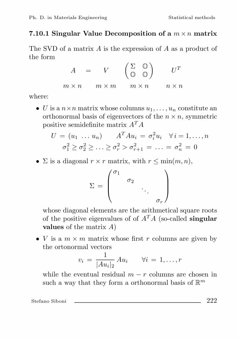
Ph. D. in Materials Engineering Statistical methods
7.10.1 Singular Value Decomposition of a m×n matrix
The SVD of a matrix A is the expression of A as a product ofthe form
A = V
(Σ O
O O
)UT
m × n m × m m × n n × n
where:
• U is a n×n matrix whose columns u1, . . . , un constitute anorthonormal basis of eigenvectors of the n× n, symmetricpositive semidefinite matrix AT A
U = (u1 . . . un) AT Aui = σ2i ui ∀ i = 1, . . . , n
σ21 ≥ σ2
2 ≥ . . . ≥ σ2r > σ2
r+1 = . . . = σ2n = 0
• Σ is a diagonal r × r matrix, with r ≤ min(m, n),
Σ =
σ1
σ2
. . .σr
whose diagonal elements are the arithmetical square rootsof the positive eigenvalues of of AT A (so-called singularvalues of the matrix A)
• V is a m × m matrix whose first r columns are given bythe ortonormal vectors
vi =1
|Aui|2Aui ∀i = 1, . . . , r
while the eventual residual m − r columns are chosen insuch a way that they form a orthonormal basis of R
m
Stefano Siboni 222

Ph. D. in Materials Engineering Statistical methods
Remark: Any m × n matrix admits a SVD!
The SVD of A
A = V
(Σ O
O O
)UT
allows us to define the so-called pseudo-inverse of A (Moore-Penrose pseudo-inverse)
A+ = U
(Σ−1
O
O O
)V T
Remark: U−1 = UT and V −1 = V T , the matrices U and Vare orthogonal by definition
If A is invertible:A+ = A−1
If not, A+ is however defined
Application
Given the linear setAx = b ,
the vectorx+ = A+b
provides the solution in the sense of the least-squares
|Ax+ − b|22 = minx∈Rn
|Ax − b|22
For an invertible A, x+ is the solution in the usual sense
Stefano Siboni 223

Ph. D. in Materials Engineering Statistical methods
7.10.2 SVD and covariance matrix of the estimatedbest-fit parameters
The matrix Φki = φk(xi)/σi, k = 1, . . . , p, i = 1, . . . , n, alsoadmits a SVD
Φ = V
(Σ O
O O
)UT
p × n p × p p × n n × n
and the structure matrix of the estimated best-fit parameters— a multivariate normal random variable — can be written
F = ΦΦT = V
(Σ2
O
O O
)V T
where all the matrices on the right-handed side are p × p
If Φ has the maximum rank — p — there holds
(Σ2
O
O O
)= Σ2
where all the diagonal entries of Σ2 are positive
Therefore the covariance matrix of the estimated best-fit pa-rameters turns out to be
F−1 = V (Σ2)−1V T
Stefano Siboni 224

Ph. D. in Materials Engineering Statistical methods
7.10.3 Example of SVD by Maple 11
The calculation is performed by the linalg Maple Package:
with(linalg);
The matrix whose SVD we want to compute is defined by:
A := linalg[matrix](2, 3, [1, 2, 3, 4, 5, 6]);
The following line
evalf(Svd(A));
provides the singular values of A:
[9.508032001, 0.7728696357]
while the matrices of the left (V ) and right (U) singular vectorsare given by:
evalf(Svd(A, V, U));
The result is displayed by
evalm(V );[−0.3863177031 −0.9223657801−0.9223657801 0.3863177031
]
and
evalm(U);−0.4286671335 0.8059639086 0.4082482905−0.5663069188 0.1123824141 −0.8164965809−0.7039467041 −0.5811990804 0.4082482905
Stefano Siboni 225

Ph. D. in Materials Engineering Statistical methods
To check the result we simply have to define the 2 × 3 matrixof the singular values
S := array(1..2, 1..3, [[9.508032001, 0, 0], [0, .7728696357, 0]]);
S :=[
9.508032001 0 00 0.7728696357 0
]
and compute then the product V SUT :
multiply(V, S, transpose(U));
[0.9999999999 2.000000000 3.0000000003.999999999 5.000000000 6.000000000
]
The matrix we obtained coincides with A up to roundoff errors,due to floating point arithmetic. The verification is successful.
Stefano Siboni 226
Ph. D. in Materials Engineering Statistical methods
7.11 Nonlinear models
They are models where the dependence on the fitting parame-ters is nonlinear
Unlike the linear models, the determination of the best-fit pa-rameters cannot be obtained analytically, by the solutionof a set of linear algebraic equations (normal equations)
The best-fit parameters must be calculated by an appropriatenumerical optimization algorithm (for the search of minima)The algorithm in of a recursive type
Optimization algorithms of current application (for search ofminima):
− steepest descent
− inverse Hessian method
− Levenberg-Marquardt method
− conjugated gradient method
− relaxation method (Barbasin-Krasovskii)
Stefano Siboni 227

Ph. D. in Materials Engineering Statistical methods
For the probability distribution of NSSAR and the joint proba-bility distribution of the best-fit parameters a1, . . . , p the sameconclusions hold we have derived for linear models providedthat the σi’s are small and that therefore the best-fit pa-rameters vary only a little
If the probability distributions of the yi’s are non-normal andwell known, the previous results are no more applicable and itis convenient to use Monte-Carlo methods
As already stressed, the troublesome change is not from linearto nonlinear models, but from normal variables to non-normalyi’s
This remark leads to the concept of “robust fitting”
Stefano Siboni 228

Ph. D. in Materials Engineering Statistical methods
7.11.1 Robust fitting
Generally speaking, a parameter estimate or a fitting are knownas “robust” if they are a little sensible to “small” deviationsfrom the hypotheses on which estimate or fitting are based
These “small deviations” may be actually “small” and concernall data
Or they may be “large” but concern only a small portion ofthe data we use for the estimate or fitting
There are many kinds of “robust” estimates
The most important ones are the so-called local M -estimates,based on the maximum likelihood principle
These provide the method for the calculation of the best-fitparameters in the “robust fitting” algorithms
Stefano Siboni 229

Ph. D. in Materials Engineering Statistical methods
Estimate of the best-fit parameters of a model by localM -estimates
If in a sequence of measurements the random errors are notnormal, the maximum likelihood method for the estimate ofthe parameters α of a model y(x, α) requires that we maximizethe quantity
P =n∏
i=1
e−ρ[yi,y(xi,α)]
where the function ρ is the natural logarithm — changed insign — of the probability distribution of the variable yi, withmean y(xi, α)
This is equivalent to minimize the sum
n∑i=1
ρ[yi, y(xi, α)]
The function often ρ[yi, y(xi, α)] depend only on the differenceyi − y(xi, α), possibly scaled by a suitable factor σi which canbe assigned to each experimental point
In that case the M -estimate is called local
The maximum likelihood condition becomes then
minα∈Rp
n∑i=1
ρ(yi − y(xi, α)
σi
)
Stefano Siboni 230

Ph. D. in Materials Engineering Statistical methods
The minimum in α (best-fit estimate a of the parameters α)can be determined directly (the mosto common procedure)
or it can be characterized as a critical point, solution of the setof equations
n∑i=1
1σi
ψ(yi − y(xi, α)
σi
)∂y(xi, α)∂aj
= 0 j = 1, . . . , p
where we have posed
ψ(z) =dρ(z)dz
∀ z ∈ R
For normal variables the function involved in the best-fitprocedure are
ρ(z) =z2
2and φ(z) = z
For variables with bilateral Gaussian distribution (orLaplace distribution)
Prob[yi − y(xi, α)] ∼ exp(−∣∣∣yi − y(xi, α)
σi
∣∣∣)we have instead
ρ(z) = |z| and φ(z) = sgn(z)
Stefano Siboni 231

Ph. D. in Materials Engineering Statistical methods
If the variables follow a Lorentz distribution (or Cauchydistribution)
Prob[yi − y(xi, α)] ∼ 1
1 +12
(yi − y(xi, α)σi
)2
the functions useful for the best-fit estimate become
ρ(z) = ln(1 +
z2
2
)e φ(z) =
z
1 +z2
2
In the analysis of data sets with moderate outliers it may beconvenient to make use of weight functions ψ which do notcorrespond to any typical probability distribution
Example I. Andrew’s sine
ψ(z) =
sin(z/c) |z| < cπ0 |z| ≥ cπ
Example II. Tukey’s biweight
ψ(z) =
z(1 − z2/c2)2 |z| < c0 z ≥ c
If the distributions are approximately normal the bestvalues of the constants c can be proved to be c = 2.1 e c = 6.0,in the two cases
Stefano Siboni 232

Ph. D. in Materials Engineering Statistical methods
7.12 Multidimensional cases
The problems of modeling in more, dependent or independent,variables can be formally treated as in the case of a uniqueindependent variable and a single dependent variable
For problems with more independent variables, the k-plesof independent variables are regarded as single variables
The sums which define the merit functions are extended overall the available k-ples
For problems with more dependent variables, the calcula-tion of merit functions is performed by treating each h-ple ofdependent variables as a vector of R
h, whose module is consid-ered (typically the usual Euclidean norm)
An important case is that of large data matrices
It is often investigated by the so-called Principal Compo-nent Analysis (PCA)
Stefano Siboni 233

Ph. D. in Materials Engineering Statistical methods
7.12.1 Principal Component Analysis (PCA)
Let X be a matrix of data, with n rows and p columns
We can assume that each of its rows corresponds to a pointin the space R
p of vectors with p components, one per eachcolumn
The matrix X specifies then a set of n points in Rp
X =
xT1
xT2
...
xTn
xi ∈ Rp ∀ i = 1, . . . , n
It may happen that the points xi are not distributed at randomin R
p, but along a particular subset of Rp
Stefano Siboni 234

Ph. D. in Materials Engineering Statistical methods
In particular, let us assume that the data are described by avector space Sk, of dimension k ≤ p, spanned by an orthonor-mal set of vectors in R
p
h1 , h2 , . . . , hk
hTj hq = δjq ∀ j, q = 1, . . . , k
Such vectors will form the columns of a matrix p × k
H =(h1
∣∣∣h2
∣∣∣ . . . ∣∣∣hk
)
Stefano Siboni 235
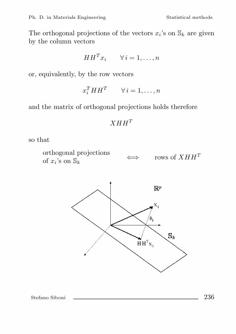
Ph. D. in Materials Engineering Statistical methods
The orthogonal projections of the vectors xi’s on Sk are givenby the column vectors
HHTxi ∀ i = 1, . . . , n
or, equivalently, by the row vectors
xTi HHT ∀ i = 1, . . . , n
and the matrix of orthogonal projections holds therefore
XHHT
so that
orthogonal projectionsof xi’s on Sk
⇐⇒ rows of XHHT
Stefano Siboni 236

Ph. D. in Materials Engineering Statistical methods
The distances of the points xi from Sk — the “residuals” —can be written
δi = xi − HHT xi = (I − HHT )xi i = 1, . . . , n
and the sum of their squares turns out to be
SS =n∑
i=1
δ2i = tr[X(I − HHT )XT ] =
= tr[XXT ] − tr[XHHTXT ] =
= tr[XXT ] − tr[HTXT XH ]
How can we determine the matrix H — or Sk?
Least-squares:we require that the matrix H — and therefore Sk — is chosenin such a way that the residual sum of squares is minimum
SS minimum
tr[HT XT XH ] maximum
with the condition that the columns h1, . . . , hk of H are or-thonormal
Stefano Siboni 237

Ph. D. in Materials Engineering Statistical methods
Result
Let us consider an orthonormal basis of eigenvectors
h1 , h2 , . . . , hp
of the real, symmetric and semipositive defined matrix
XT X
with
XT Xhi = λihi ∀ i = 1, . . . , p
and eigenvalues arranged in decreasing order
λ1 ≥ λ2 ≥ . . . ≥ λp ≥ 0
Then
• we can poseH =
(h1
∣∣∣h2
∣∣∣ . . . ∣∣∣hk
)
• the corresponding (residual) sum of squares holds
tr[X(I − HHT )XT ] =p∑
i=k+1
λi
Stefano Siboni 238

Ph. D. in Materials Engineering Statistical methods
If we conjecture that the data xi are principally located alongSk, we replace the points xi with their orthogonal projectionson Sk
xi −−−−−−→ HHTxi
so that the data matrix X is replaced with the k-principalcomponent model
XHHT =k∑
j=1
(Xhj)hTj
(so-called calibration of the k-principal component model)
The sum of squares of data (“deviance of the sample”)
n∑i=1
p∑j=1
x2ij = tr(XT X) =
p∑j=1
λj
is composed by a “deviance explained by the model”
tr[XHHTXT ] = tr[HT XT XH ] =k∑
j=1
λj
and a “unexplained deviance” or (residual) sum of squares
SS = tr[X(I − HHT )XT ] =p∑
j=k+1
λj
Stefano Siboni 239

Ph. D. in Materials Engineering Statistical methods
If the k-principal component model is correct
all the data vectors x ∈ Rp can be represented as linear com-
binations of the orthonormal eigenvectors h1, . . . , hk:
x =k∑
j=1
αjhj
with α1, . . . , αk ∈ R
This allows us to express p− k components of x as linear func-tions of the remaining k components
For instance, the first p − k as a function of the last k:
x1 = f1(xp−k+1, . . . , xp)x2 = f2(xp−k+1, . . . , xp). . . . . .
xp−k = fp−k(xp−k+1, . . . , xp)
The k-principal component model allows us to predict the val-ues of p − k components of the datum x ∈ R
p, whenever theremaining k components are known!
(use of the k-principal component model for prediction)
Stefano Siboni 240

Ph. D. in Materials Engineering Statistical methods
By comparison, we can easily verify that the k-principal com-ponent model is no more than a truncation to the largest ksingular values of the SVD of X
X = V
(Σ O
O O
)UT =
r∑j=1
σjvjuTj
with:
− r = Rank(X) = Rank(XT X) ≤ min(n, p)
− U =(u1
∣∣∣u2
∣∣∣ . . . ∣∣∣up
)u1, u2, . . . , up orthonormal basis of eigenvectors of XT X
XT Xui = σ2i ui i = 1, . . . , p
according to the eigenvalues of XT X arranged in a de-creasing order
σ21 ≥ σ2
2 ≥ . . . ≥ σ2p
− andV =
(v1
∣∣∣v2
∣∣∣ . . . ∣∣∣vn
)v1, v2, . . . , vn orthonormal basis of R
n such that
vi =1σi
Xui ∀ i = 1, . . . , r
Therefore, if k ≤ r — the only interesting case — we havek∑
j=1
σjvjuTj =
k∑j=1
σj1σj
(Xuj)uTj =
k∑j=1
(Xuj)uTj
and to obtain the k-principal component model it is enough topose hj = uj ∀ j = 1, . . . , k. Moreover, there holds λj = σ2
j
∀ j = 1, . . . , k.
Stefano Siboni 241

Ph. D. in Materials Engineering Statistical methods
The k-principal component model of the matrix X is thus givenby
XHHT =k∑
j=1
(Xhj)hTj
with:
• hi i-th principal component (loading)
and
• Xhi i-th score
Remark The PCA is nothing else than a truncated SVD
The algorithms for the PCA are therefore the same of the SVD!
Stefano Siboni 242
Ph. D. in Materials Engineering Statistical methods
7.12.2 PCA for non-centred data (General PCA)
We can also attempt to model the data matrix X
by a linear manifold of dimension k(or k-dimensional hyperplane of R
p)
which does not pass through the origin O
and thus does not constitute a vector subspace of Rp, like Sk
It can be proved that the result is still obtained by the previousprocedure
provided that, however, the appropriate means are subtractedto all the points xi
xi − x = xi −1n
n∑q=1
xq
or, equivalently, that the analysis is performed on the “centred”data matrix
X − NX = (I − N )X
where N denotes the n × n matrix of constant entries
Nij =1n
∀ i, j = 1, . . . , n
(The proof follows an argument similar to that of Huygens-Steiner theorem in theoretical mechanics)
Stefano Siboni 243

Ph. D. in Materials Engineering Statistical methods
8. Summary of useful Maple 11 and Excel commands
(•) Calculation of t[α](n)
Maple 11:with(stats):statevalf[icdf, students[n]](α);
Excel: TINV(2 − 2α; n)
(•) Calculation of X 2[α](n)
Maple 11:with(stats):statevalf[icdf, chisquare[n]](α);
Excel: CHIINV(1 − α; n)
(•) Calculation of z[α]
Maple 11:with(stats):statevalf[icdf, normald[0, 1]](α);
Excel: NORMINV(α; 0; 1)
(•) Calculation of F[α](n1 ,n2)
Maple 11:with(stats):statevalf[icdf, fratio[n1, n2]](α);
Excel: FINV(1 − α; n1; n2)
(•) Goodness of fit Q for a regression model with n − p d.o.f.
Maple 11: 1 − stats[statevalf , cdf , chisquare[n− p]](NSSAR);
Excel: CHIDIST(NSSAR; n− p)
Stefano Siboni 244

Ph. D. in Materials Engineering Statistical methods
List of topics
1. Experimental errors . . . . . . . . . . . . . . . . . . . . . . . . . . . . . . . . 12. Random variables . . . . . . . . . . . . . . . . . . . . . . . . . . . . . . . . . . 42.1 General definitions and properties . . . . . . . . . . . . . . . . . . 42.2 Examples of discrete RVs . . . . . . . . . . . . . . . . . . . . . . . . . . . 72.3 Examples of continuous RVs . . . . . . . . . . . . . . . . . . . . . . . . 82.4 Remark. Relevance of normal variables . . . . . . . . . . . . . 162.5 Probability distributions in more dimensions . . . . . . . . 182.5.1 (Stochastically) independent RVs . . . . . . . . . . . . . . . . . . . 192.5.2 (Stochastically) dependent RVs . . . . . . . . . . . . . . . . . . . . . 192.5.3 Mean, covariance, correlation of a set of RVs . . . . . . . . 202.5.4 Multivariate normal (or Gaussian) RVs . . . . . . . . . . . . . 223. Indirect measurements. Functions of RVs . . . . . . . . . . . 253.1 Generalities . . . . . . . . . . . . . . . . . . . . . . . . . . . . . . . . . . . . . . . . 253.2 Linear combination of RVs . . . . . . . . . . . . . . . . . . . . . . . . . 273.3 Linear combination of multivariate normal RVs . . . . . 283.4 Quadratic forms of standard variables . . . . . . . . . . . . . . 303.4.1 Craig theorem . . . . . . . . . . . . . . . . . . . . . . . . . . . . . . . . . . . . . . 303.4.2 Characterization theorem of chi-square RVs . . . . . . . . . 303.4.3 Fisher-Cochran theorem . . . . . . . . . . . . . . . . . . . . . . . . . . . . 323.4.4 Two-variable cases . . . . . . . . . . . . . . . . . . . . . . . . . . . . . . . . . 333.5 Error propagation in indirect measurements . . . . . . . . 343.5.1 Gauss law . . . . . . . . . . . . . . . . . . . . . . . . . . . . . . . . . . . . . . . . . . 353.5.2 Logarithmic differential . . . . . . . . . . . . . . . . . . . . . . . . . . . . 363.5.3 Error propagation in solving a set
of linear algebraic equations . . . . . . . . . . . . . . . . . . . . . . . . 383.5.4 Probability distribution of a function of RVs
estimated by Monte-Carlo methods . . . . . . . . . . . . . . . . . 444. Sample theory. Sample estimates of µ and σ2 . . . . . . . 484.1 Sample estimate of the mean µ . . . . . . . . . . . . . . . . . . . . . 49
Stefano Siboni -1

Ph. D. in Materials Engineering Statistical methods
4.2 Sample estimate of the variance σ2 . . . . . . . . . . . . . . . . . 524.3 Normal RVs. Confidence intervals for µ and σ2 . . . . . 544.3.1 Confidence interval for the mean µ . . . . . . . . . . . . . . . . . 564.3.2 Confidence interval for the variance σ2 . . . . . . . . . . . . . 584.4 Large samples of an arbitrary population.
Approximate confidence intervals of µ and σ2 . . . . . . . 624.4.1 Confidence interval for the mean µ . . . . . . . . . . . . . . . . . 624.4.2 Confidence interval for the variance σ2 . . . . . . . . . . . . . 625. Hypothesis testing . . . . . . . . . . . . . . . . . . . . . . . . . . . . . . . . . 705.1 X 2-test for adapting a distribution to a sample . . . . . 785.2 Kolmogorov-Smirnov test . . . . . . . . . . . . . . . . . . . . . . . . . . 865.2.1 Remark. Calculation of the KS variable . . . . . . . . . . . . 945.2.2 Remark. The KS probability distribution is
independent on the cumulative distribution P (x) ofthe random variable on which the test is performed . 95
5.3 t-test on the mean of a normal population . . . . . . . . . . 965.4 X 2-test on the variance of a normal population . . . . . 1015.5 z-test to compare the means of two independent
normal populations (of known variances) . . . . . . . . . . . 1065.6 F -test to compare the variances of two independent
normal populations . . . . . . . . . . . . . . . . . . . . . . . . . . . . . . . . . 1075.7 Unpaired t-test to compare the means of two
independent normal populations (unknown variances) 1145.7.1 Case of equal variances: σ2
1 = σ22 = σ2 . . . . . . . . . . . . . . 114
5.7.2 Case of unequal variances: σ21 = σ2
2 . . . . . . . . . . . . . . . . . 1155.7.3 Remark for the case σ2
1 = σ22 . Proof that the test
variable actually follows a Student’s distributionwith p + q − 2 d.o.f. . . . . . . . . . . . . . . . . . . . . . . . . . . . . . . . . 116
5.8 Paired t-test to compare the means of twonormal populations (unknown variances) . . . . . . . . . . . 120
5.9 F -test for the comparison of means . . . . . . . . . . . . . . . . . 124
Stefano Siboni -2

Ph. D. in Materials Engineering Statistical methods
5.9.1 1-factor ANOVA . . . . . . . . . . . . . . . . . . . . . . . . . . . . . . . . . . . 1285.9.2 2-factor ANOVA . . . . . . . . . . . . . . . . . . . . . . . . . . . . . . . . . . . 1355.9.3 2-factor ANOVA without interaction . . . . . . . . . . . . . . . 1385.9.4 2-factor ANOVA with interaction . . . . . . . . . . . . . . . . . . . 1445.10 Sign test for the median of a population . . . . . . . . . . . . 1465.11 Sign test to check if two paired samples
belong to the same population . . . . . . . . . . . . . . . . . . . . . . 1485.12 Detection of outliers by Chauvenet criterion . . . . . . . . 1526. Pairs of random variables . . . . . . . . . . . . . . . . . . . . . . . . . . . 1576.1 Linear correlation coefficient (Pearson r) . . . . . . . . . . . . 1576.2 Statistics of the linear correlation coefficient . . . . . . . . 1616.2.1 Independent random variables (x, y) . . . . . . . . . . . . . . . . 1626.2.2 Normal random variables (x, y) . . . . . . . . . . . . . . . . . . . . . 1636.2.2.1 Approximation for large n. Fisher transformation . . . 1646.2.2.2 Independent (or uncorrelated) normal variables . . . . . 1646.3 Remark. . . . . . . . . . . . . . . . . . . . . . . . . . . . . . . . . . . . . . . . . . . . 1697. Data modelling . . . . . . . . . . . . . . . . . . . . . . . . . . . . . . . . . . . . 1707.1 General setup of the problem . . . . . . . . . . . . . . . . . . . . . . . 1707.2 Linear regression by the chi-square method
(chi-square fitting) . . . . . . . . . . . . . . . . . . . . . . . . . . . . . . . . . 1747.2.1 Optimization. Normal equation and its solution . . . . 1767.2.2 The parameters of the linear regression,
estimated by chi-square fitting, as RVs . . . . . . . . . . . . . 1777.2.3 Goodness of fit . . . . . . . . . . . . . . . . . . . . . . . . . . . . . . . . . . . . . 1787.2.4 Remark. Standard deviations σi unknown . . . . . . . . . . 1817.3 F -test for the goodness of fit . . . . . . . . . . . . . . . . . . . . . . . 1827.4 F -test with repeated measurements on y . . . . . . . . . . . . 1877.4.1 Known variances σ2
i . . . . . . . . . . . . . . . . . . . . . . . . . . . . . . . . 1887.4.2 Equal (although unknown) variances σ2
i . . . . . . . . . . . . 1907.5 Incremental F -test . . . . . . . . . . . . . . . . . . . . . . . . . . . . . . . . . 1917.6 Confidence intervals for the regression parameters . . 193
Stefano Siboni -3

Ph. D. in Materials Engineering Statistical methods
7.7 Confidence intervals for predictions . . . . . . . . . . . . . . . . . 1937.8 Important case. Regression straight line . . . . . . . . . . . . 1957.10 Chi-square fitting by Singular Value Decomposition . 2217.10.1 Singular Value Decomposition of a m × n matrix . . . 2227.10.2 SVD and covariance matrix
of the estimated best-fit parameters . . . . . . . . . . . . . . . . 2247.10.3 Example of SVD by Maple 11 . . . . . . . . . . . . . . . . . . . . . . 2257.11 Nonlinear models . . . . . . . . . . . . . . . . . . . . . . . . . . . . . . . . . . 2277.11.1 Robust fitting . . . . . . . . . . . . . . . . . . . . . . . . . . . . . . . . . . . . . . 2297.12 Multidimensional cases . . . . . . . . . . . . . . . . . . . . . . . . . . . . . 2337.12.1 Principal Component Analysis (PCA) . . . . . . . . . . . . . . 2347.12.2 PCA for non-centred data (General PCA) . . . . . . . . . . 2438. Summary of useful Maple 11 and Excel commands . . 244
Stefano Siboni -4