Metropolis Light Transport

Eric Veach Leonidas J. Guibas

Computer Science DepartmentStanford University

Abstract

We present a new Monte Carlo method for solving thelight transport problem, inspired by the Metropolis samplingmethod in computational physics. To render an image, wegenerate a sequence of light transport paths by randomlymutating a single current path (e.g. adding a new vertex tothe path). Each mutation is accepted or rejected with a care-fully chosen probability, to ensure that paths are sampledaccording to the contribution they make to the ideal image.We then estimate this image by sampling many paths, andrecording their locations on the image plane.

Our algorithm is unbiased, handles general geometric andscattering models, uses little storage, and can be orders ofmagnitude more efficient than previous unbiased approaches.It performs especially well on problems that are usually con-sidered difficult, e.g. those involving bright indirect light,small geometric holes, or glossy surfaces. Furthermore, itis competitive with previous unbiased algorithms even forrelatively simple scenes.

The key advantage of the Metropolis approach is that thepath space is explored locally, by favoring mutations thatmake small changes to the current path. This has severalconsequences. First, the average cost per sample is small(typically only one or two rays). Second, once an impor-tant path is found, the nearby paths are explored as well,thus amortizing the expense of finding such paths over manysamples. Third, the mutation set is easily extended. By con-structing mutations that preserve certain properties of thepath (e.g. which light source is used) while changing others,we can exploit various kinds of coherence in the scene. It isoften possible to handle difficult lighting problems efficientlyby designing a specialized mutation in this way.

CR Categories: I.3.7 [Computer Graphics]: Three-Dimensional Graphics and Realism; I.3.3 [Computer Graph-ics]: Picture/Image Generation; G.1.9 [Numerical Analysis]:Integral Equations—Fredholm equations.

Keywords: global illumination, lighting simulation,radiative heat transfer, physically-based rendering, MonteCarlo integration, variance reduction, Metropolis-Hastingsalgorithm, Markov Chain Monte Carlo (MCMC) methods

E-mail: ericv@cs.stanford.edu, guibas@cs.stanford.edu

1 Introduction

There has been a great deal of work in graphics on solv-ing the light transport problem efficiently. However, cur-rent methods are optimized for a fairly narrow class of inputscenes. For example, many algorithms require a huge in-crease in computer resources when there is bright indirectlighting, or when most surfaces are non-diffuse reflectors.For light transport algorithms to be widely used, it is im-portant to find techniques that are less fragile. Renderingalgorithms must run within acceptable time bounds on realmodels, yielding images that are physically plausible andvisually pleasing. They must support complex geometry,materials, and illumination — these are all essential compo-nents of real-life environments.

Monte Carlo methods are an attractive starting point inthe search for such algorithms, because of their general-ity and simplicity. Especially appealing are unbiased algo-rithms, i.e. those that compute the correct answer on theaverage. For these algorithms, any error in the solution isguaranteed to show up as random variations among the sam-ples (e.g., as image noise). This error can be estimated bysimply computing the sample variance.

On the other hand, many methods used in graphics arebiased. To make any claims about the correctness of the re-sults of these algorithms, we must bound the amount of bias.In general this is very difficult to do; it cannot be estimatedby simply drawing a few more samples. Biased algorithmsmay produce results that are not noisy, but are neverthe-less incorrect. This error is often noticeable visually, in theform of discontinuities, excessive blurring, or objectionablesurface shading.

In graphics, the first unbiased Monte Carlo light transportalgorithm was proposed by Kajiya [10], building on earlierwork by Cook et al. [4] and Whitted [26]. Since then manyrefinements have been suggested (e.g. see [1]). Often theseimprovements have been adapted from the neutron transportand radiative heat transfer literatures, which have a longhistory of solving similar problems [22].

However, it is surprisingly difficult to design light trans-port algorithms that are general, efficient, and artifact-free.1

From a Monte Carlo viewpoint, such an algorithm must effi-ciently sample the transport paths from the light sources tothe lens. The problem is that for some environments, mostpaths do not contribute significantly to the image, e.g. be-cause they strike surfaces with low reflectivity, or go throughsolid objects. For example, imagine a brightly lit room nextto a dark room containing the camera, with a door slightlyajar between them. Naive path tracing will be very ineffi-cient, because it will have difficulty generating paths that

1In this regard, certain ray-tracing problems have been shownto be undecidable, i.e. they cannot be solved on a Turing machine[19]. We can expect that any light transport algorithm will per-form very badly as the geometry and materials of the input sceneapproach a provably difficult configuration.

go through the doorway. Similar problems occur when thereare glossy surfaces, caustics, strong indirect lighting, etc.

Several techniques have been proposed to sample thesedifficult paths more efficiently. One is bidirectional pathtracing, developed independently by Lafortune and Willems[12, 13], and Veach and Guibas [24, 25]. These methodsgenerate one subpath starting at a light source and anotherstarting at the lens, then they consider all the paths ob-tained by joining every prefix of one subpath to every suffixof the other. This leads to a family of different importancesampling techniques for paths, which are then combined tominimize variance [25]. This can be an effective solution forcertain kinds of indirect lighting problems.

Another idea is to build an approximate representationof the radiance in a scene, which is then used to modifythe directional sampling of the basic path tracing algorithm.This can be done with a particle tracing prepass [9], or byadaptively recording the radiance information in a spatialsubdivision [14]. Moderate variance reductions have beenreported (50% to 70%), but there are several problems, in-cluding inadequate directional resolution to handle concen-trated indirect lighting, and substantial space requirements.Similar ideas have been applied to particle tracing [17, 5].

We propose a new algorithm for importance samplingthe space of paths, which we call Metropolis light transport(MLT). The algorithm samples paths according to the con-tribution they make to the ideal image, by means of a ran-dom walk through path space. In Section 2, we give a high-level overview of MLT, then we describe its components indetail. Section 3 summarizes the classical Metropolis sam-pling algorithm, as developed in computational physics. Sec-tion 4 describes the path integral formulation of light trans-port, upon which our methods are based. Section 5 showshow to combine these two ideas to yield an effective lighttransport algorithm. Results are presented in Section 6, fol-lowed by conclusions and suggested extensions in Section 7.To our knowledge, this is the first application of the Metrop-olis method to transport problems of any kind.

2 Overview of the MLT algorithm

To make an image, we sample the paths from the lightsources to the lens. Each path x is a sequence x0x1 . . .xk ofpoints on the scene surfaces, where k ≥ 1 is the length of thepath (the number of edges). The numbering of the verticesalong the path follows the direction of light flow.

We will show how to define a function f on paths, togetherwith a measure µ, such that

∫Df(x) dµ(x) represents the

power (flux) that flows from the light sources to the imageplane along a set of paths D. We call f the image contribu-tion function, since f(x) is proportional to the contributionmade to the image by light flowing along x.

Our overall strategy is to sample paths with probabilityproportional to f , and record the distribution of paths overthe image plane. To do this, we generate a sequence of pathsX0, X1, . . ., XN , where each Xi is obtained by a randommutation to the path Xi−1. The mutations can have almostany desired form, and typically involve adding, deleting, orreplacing a small number of vertices on the current path.

However, each mutation has a chance of being rejected,depending on the relative contributions of the old and newpaths. For example, if the new path passes through a wall,the mutation will be rejected (by setting Xi = Xi−1). TheMetropolis framework gives a recipe for determining the ac-ceptance probability for each mutation, such that in the limit

the sampled paths Xi are distributed according to f (this isthe stationary distribution of the random walk).

As each path is sampled, we update the current image(which is stored in memory as a two-dimensional array ofpixel values). To do this, we find the image location (u, v)corresponding to each path sample Xi, and update the val-ues of those pixels whose filter support contains (u, v). Allsamples are weighted equally; the light and dark regions ofthe final image are caused by differences in the number ofsamples recorded there.

The MLT algorithm is summarized below. In the followingsections, we will describe it in more detail.

x← InitialPath()image← array of zeros for i← 1 to N

y←Mutate(x)

a← AcceptProb(y|x)if Random() < a

then x← yRecordSample(image, x)

return image

3 The Metropolis sampling algorithm

In 1953, Metropolis, Rosenbluth, Rosenbluth, Teller, andTeller introduced an algorithm for handling difficult sam-pling problems in computational physics [15]. It was origi-nally used to predict the material properties of liquids, buthas since been applied to many areas of physics and chem-istry.

The method works as follows (our discussion is based on[11]). We are given a state space Ω, and a non-negativefunction f : Ω → IR+. We are also given some initial stateX0 ∈ Ω. The goal is to generate a random walk X0, X1, . . .such that Xi is eventually distributed proportionally to f , nomatter which state X0 we start with. Unlike most samplingmethods, the Metropolis algorithm does not require that fintegrate to one.

Each sample Xi is obtained by making a random change toXi−1 (in our case, these are the path mutations). This typeof random walk, where Xi depends only on Xi−1, is calleda Markov chain. We let K(y | x) denote the probabilitydensity of going to state y, given that we are currently instate x. This is called the transition function, and satisfiesthe condition

∫ΩK(y | x) dµ(y) = 1 for all x ∈ Ω.

The stationary distribution. Each Xi is a random variablewith some distribution pi, which is determined from pi−1 by

pi(x) =

∫Ω

K(x | y) pi−1(y) dµ(y) . (1)

With mild conditions onK (discussed further in Section 5.2),the pi will converge to a unique distribution p, called thestationary distribution. Note that p does not depend on theinitial state X0.

To give a simple example of this idea, consider a statespace consisting of n2 vertices arranged in an n×n grid. Eachvertex is connected to its four neighbors by edges, wherethe edges “wrap” from left to right and top to bottom asnecessary (i.e. with the topology of a torus). A transitionconsists of randomly moving from the current vertex x toone of the neighboring vertices y with a probability of 1/5each, and otherwise staying at vertex x.

Suppose that we start at an arbitrary vertex X0 = x∗, sothat p0(x)=1 for x= x∗, and p0(x)=0 otherwise. After onetransition, X1 is distributed with equal probability among x∗

and its four neighbors. Similarly, X2 is randomly distributedamong 13 vertices (although not with equal probability). Ifthis process is continued, eventually pi converges to a fixedprobability distribution p, which necessarily satisfies

p(x) =∑

yK(x | y) p(y) .

For this example, p is the uniform distribution p(x)=1/n2.

Detailed balance. In a typical physical system, the transi-tion function K is determined by the physical laws governingthe system. Given some arbitrary initial state, the systemthen evolves towards equilibrium through transitions gov-erned by K.

The Metropolis algorithm works in the opposite direction.The idea is to invent or construct a transition function Kwhose resulting stationary distribution will be proportionalto the given f , and which will converge to f as quickly aspossible. The technique is simple, and has an intuitive phys-ical interpretation called detailed balance.

Given Xi−1, we obtain Xi as follows. First, we choosea tentative sample X′i , which can be done in almost anyway desired. This is represented by the tentative transitionfunction T , where T (y | x) gives the probability density thatX′i= y given that Xi−1 = x.

The tentative sample is then either accepted or rejected,according to an acceptance probability a(y | x) which will bedefined below. That is, we let

Xi =

X′i with probability a(X′i |Xi−1) ,Xi−1 otherwise .

(2)

To see how to set a(y | x), suppose that we have alreadyreached equilibrium, i.e. pi−1 is proportional to f . We mustdefine K(y | x) such that the equilibrium is maintained. Todo this, consider the density of transitions between any twostates x and y. From x to y, the transition density is pro-portional to f(x) T (y | x) a(y | x), and a similar statementholds for the transition density from y to x. To maintainequilibrium, it is sufficient that these densities be equal:

f(x) T (y | x) a(y | x) = f(y) T (x | y) a(x | y) , (3)

a condition known as detailed balance. We can verify thatif pi−1 ∝ f and condition (3) holds, then equilibrium ispreserved:

pi(x) =[1−

∫Ωa(y | x) T (y | x) dµ(y)

]pi−1(x) (4)

+∫

Ωa(x | y) T (x | y) pi−1(y) dµ(y)

= pi−1(x) .

The acceptance probability. Recall that f is given, and Twas chosen arbitrarily. Thus, equation (3) is a condition onthe ratio a(y | x)/a(x | y). In order to reach equilibrium asquickly as possible, the best strategy is to make a(y | x) anda(x | y) as large as possible [18], which is achieved by letting

a(y | x) = min

1,f(y) T (x | y)

f(x) T (y | x)

. (5)

According to this rule, transitions in one direction are alwaysaccepted, while in the other direction they are sometimesrejected, such that the expected number of moves each wayis the same.

Comparison with genetic algorithms. The Metropolismethod differs from genetic algorithms [6] in several ways.First, they have different purposes: genetic algorithms solveoptimization problems, while the Metropolis method solvessampling problems (there is no search for an optimum value).Genetic algorithms work with a population of individuals,while Metropolis stores only a single current state. Finally,genetic algorithms have much more freedom in choosing theallowable mutations, since they do not need to compute theconditional probability of their actions.

Beyer and Lange [2] have applied genetic algorithms to theproblem of integrating radiance over a hemisphere. Theystart with a population of rays (actually directional sam-ples), which are evolved to improve their distribution withrespect to the incident radiance at a particular surface point.However, their methods do not seem to lead to a feasiblelight transport algorithm.

4 The path integral formulation of lighttransport

Often the light transport problem is written as an integralequation, where we must solve for the equilibrium radiancefunction L. However, it can also be written as a pure inte-gration problem, over the domain of all transport paths. TheMLT algorithm is based on this formulation.2 We start byreviewing the light transport and measurement equations,and then show how to transform them into an integral overpaths.

The light transport equation. We assume a geometric op-tics model where light is emitted, scattered, and absorbedonly at surfaces, travels in straight lines between surfaces,and is perfectly incoherent. Under these conditions, the lighttransport equation is given by3

L(x′→x′′) =Le(x′→x′′) (6)

+

∫ML(x→x′) fs(x→x′→x′′)G(x↔x′) dA(x).

HereM is the union of all scene surfaces, A is the area mea-sure onM, Le(x′→x′′) is the emitted radiance leaving x′ inthe direction of x′′, L is the equilibrium radiance function,and fs is the bidirectional scattering distribution function(BSDF). The notation x→ x′ symbolizes the direction oflight flow between two points of M, while x↔ x′ denotessymmetry in the argument pair.4 The function G representsthe throughput of a differential beam between dA(x) anddA(x′), and is given by

G(x↔x′) = V (x↔x′)| cos(θo) cos(θ′i)|‖x− x′‖2 ,

where θo and θ′i represent the angles between the segmentx↔ x′ and the surface normals at x and x′ respectively,while V (x↔x′) = 1 if x and x′ are mutually visible and iszero otherwise.

2Note that two different formulations of bidirectional pathtracing have been proposed: one based on a measure over paths[24, 25], and the other based on the global reflectance distributionfunction (GRDF) [13]. However, only the path measure approachdefines the notion of probabilities on paths, as required for com-bining multiple estimators [25] and the present work.

3Technically, the equations of this section deal with spectralradiance, and apply at each wavelength separately.

4There is redundancy in this representation; e.g. L(x→x′) =L(x→x′′) whenever x′ and x′′ lie in the same direction from x.

The measurement equation. Light transport algorithmsestimate a finite number of measurements of the equilibriumradiance L. We consider only algorithms that compute animage directly, so that the measurements consist of manypixel values m1, . . . ,mM , where M is the number of pixelsin the image. Each measurement has the form

mj =

∫M×M

W (j)e (x→x′)L(x→x′)G(x↔x′) dA(x) dA(x′),

(7)

where W (j)e (x→x′) is a weight that indicates how much the

light arriving at x′ from the direction of x contributes to thevalue of the measurement.5 For real sensors, W (j)

e is calledthe flux responsivity (with units of [W−1]), but in graphicsit is more often called an importance function.6

The path integral formulation. By recursively expandingthe transport equation (6), we can write measurements inthe form

mj =

∫M2

Le(x0→x1)G(x0↔x1)W(j)

e (x0→x1) dA(x0) dA(x1)

+

∫M3Le(x0→x1)G(x0↔x1) fs(x0↔x1↔x2)

G(x1↔x2)W (j)e (x1→x2) dA(x0) dA(x1) dA(x2)

+· · · . (8)

The goal is to write this expression in the form

mj =

∫Ω

fj(x) dµ(x) , (9)

so that we can handle it as a pure integration problem.To do this, let Ωk be the set of all paths of the form

x = x0x1 . . .xk, where k ≥ 1 and xi ∈ M for each i. Wedefine a measure µk on the paths of each length k accordingto

dµk(x0 . . .xk) = dA(x0) · · · dA(xk) ,

i.e. µk is a product measure. Next, we let Ω be the union ofall the Ωk, and define a measure µ on Ω by7

µ(D) =

∞∑k=1

µk(D ∩Ωk) . (10)

The integrand fj is defined by extracting the appropriateterm from the expansion (8) — see Figure 1. For example,

fj(x0x1) = Le(x0→x1) G(x0↔x1) W (j)e (x0→x1) .

We call fj the measurement contribution function.There is nothing tricky about this; we have just expanded

and rearranged the transport equations. The most signifi-cant aspect is that we have removed the sum over differentpath lengths, and replaced it with a single integral over anabstract measure space of paths.

5The function W (j)e is zero almost everywhere. It is non-zero

only if x′ lies on the virtual camera lens, and the ray x → x′

is mapped by the lens to the small region of the image planecorresponding to the filter support of pixel j.

6Further references and discussion may be found in [23].7This measure on paths is similar to that of Spanier and Gel-

bard [22, p. 85]. However, in our case infinite-length paths areexcluded. This makes it easy to verify that (10) is in fact a mea-sure, directly from the axioms [7].

We(x2, x3)

fs(x0, x1, x2)

fs(x1, x2, x3)

G(x0, x1)

Le(x0, x1)

G(x1, x2)G(x2, x3)

x0x1

x2

x3

Figure 1: The measurement contribution function fj is aproduct of many factors (shown for a path of length 3).

5 Metropolis light transport

To complete the MLT algorithm outlined in Section 2, thereare several tasks. First, we must formulate the light trans-port problem so that it fits the Metropolis framework. Sec-ond, we must show how to avoid start-up bias, a problemwhich affects many Metropolis applications. Most impor-tantly, we must design a suitable set of mutations on paths,such that the Metropolis method will work efficiently.

5.1 Reduction to the Metropolis framework

We show how the Metropolis method can be adapted to es-timate all of the pixel values mj simultaneously and withoutbias.

Observe that each integrand fj has the form

fj(x) = wj(x) f(x) , (11)

where wj represents the filter function for pixel j, and frepresents all the other factors of fj (which are the same forall pixels). In physical terms,

∫Df(x) dµ(x) represents the

radiant power received by the image area of the image planealong a set D of paths.8 Note that wj depends only on thelast edge xk−1xk of the path, which we call the lens edge.

An image can now be computed by sampling N paths Xiaccording to some distribution p, and using the identity

mj = E

[1

N

N∑i=1

wj(Xi)f(Xi)

p(Xi)

].

If we could let p = (1/b) f (where b is the normalizationconstant

∫Ωf(x) dµ(x)), the estimate for each pixel would

be

mj = E

[1

N

N∑i=1

b wj(Xi)

].

This equation can be evaluated efficiently for all pixels atonce, since each path contributes to only a few pixel values.

This idea requires the evaluation of b, and the ability tosample from a distribution proportional to f . Both of theseare hard problems. For the second part, the Metropolis al-gorithm will help; however, the samples Xi will have thedesired distribution only in the limit as i→∞. In typicalMetropolis applications, this is handled by starting in somefixed initial state X0, and discarding the first k samples untilthe random walk has approximately converged to the equi-librium distribution. However, it is often difficult to knowhow large k should be. If it is too small, then the sampleswill be strongly influenced by the choice of X0, which willbias the results (this is called start-up bias).

8We assume that f(x)=0 for paths that do not contribute toany pixel value (so that we do not waste any samples there).

Eliminating start-up bias. We show how the MLT algo-rithm can be initialized to avoid start-up bias. The ideais to start the walk in a random initial state X0, which issampled from some convenient path distribution p0 (we usebidirectional path tracing for this purpose). To compensatefor the fact that p0 is not the desired distribution (1/b) f ,the sample X0 is assigned a weight: W0 = f(X0)/p0(X0).Thus after one sample, the estimate for pixel j is W0wj(X0).All of these quantities are computable since X0 is known.

Additional samples X1, X2, . . ., XN are generated by mu-tating X0 according to the Metropolis algorithm (using f asthe target density). Each of the Xi has a different distribu-tion pi, which only approaches (1/b) f as i→∞. To avoidbias, however, it is sufficient to assign these samples the sameweight Wi=W0 as the original sample, where the followingestimate is used for pixel j:

mj = E

[1

N

N∑i=1

Wi wj(Xi)

]. (12)

To show that this is unbiased, recall that the initial statewas chosen randomly, and so we must average over all choicesof X0 when computing expected values. Consider a group ofstarting paths obtained by sampling p0 many times. If wehad p0 = (1/b) f and W0 = b, then obviously this startinggroup would be in equilibrium. For general p0, the choiceW0 = f/p0 leads to exactly the same distribution of weightamong the starting paths, and so we should expect that theseinitial conditions are unbiased as well. (See Appendix A fora proof.)

This technique for removing start-up bias is not specificto light transport. However, it requires the existence of analternative sampling method p0, which for many Metropolisapplications is not easy to obtain.

Initialization. In practice, initializing the MLT algorithmwith a single sample does not work well. If we generate onlyone path X0 (e.g. using bidirectional path tracing), it is quitelikely that W0 =0 (e.g. the path goes through a wall). Sinceall subsequent samples use the same weight Wi =W0, thiswould lead to a completely black final image. Conversely,the initial weight W0 on other runs may be much largerthan expected. Although the algorithm is unbiased, thisstatement is only useful when applied to the average resultover many runs. The obvious solution is to run n copiesof the algorithm in parallel, and accumulate all the samplesinto one image.

The strategy we have implemented is to sample a moder-ately large number of paths X(1)

0 , . . ., X(n)0 , with correspond-

ing weights W (1)0 , . . ., W (n)

0 . We then resample the X(i)0 to

obtain a much smaller number n′ of equally-weighted paths(chosen with equal spacing in the cumulative weight distri-

bution of the X(i)0 ). These are used as independent seeds for

the Metropolis phase of the algorithm.The value of n is determined indirectly, by generating a

fixed number of eye and light subpaths (e.g. 10 000 pairs),and considering all the ways to link the vertices of each pair.Note that it is not necessary to save all of these paths forthe resampling step; they can be regenerated by restartingthe random number generator with the same seed.

It is often reasonable to choose n′ = 1 (a single Metrop-olis seed). In this case, the purpose of the first phase is toestimate the mean value of W0, which determines the ab-solute image brightness.9 If the image is desired only up

9More precisely, E[W0] =∫f = b, which represents the total

power falling on the image region of the film plane.

to a constant scale factor, then n can be chosen to be verysmall. The main reasons for retaining more than one seed(i.e. n′ > 1) are to implement convergence tests (see below)or lens subpath mutations (Section 5.3.3).

Effectively, we have separated the image computation intotwo subproblems. The initialization phase estimates theoverall image brightness, while the Metropolis phase deter-mines the relative pixel intensities across the image. Theeffort spent on each phase can be decided independently.In practice, however, the initialization phase is a negligiblepart of the total computation time (e.g., even 100 000 bidi-rectional samples typically constitute less than one sampleper pixel).

Convergence tests. Another reason to run several copiesof the algorithm in parallel is that it facilitates convergencetesting. (We cannot apply the usual variance tests to sam-ples generated by a single run of the Metropolis algorithm,since consecutive samples are highly correlated.)

To test for convergence, the Metropolis phase runs withn′ independent seed paths, whose contributions to the imageare recorded separately (in the form of n′ separate images).This is done only for a small representative fraction of thepixels, since it would be too expensive to maintain manycopies of a large image. The sample variance of these testpixels is then computed periodically, until the results arewithin prespecified bounds.10

Spectral sampling. Our discussion so far has been limitedto monochrome images, but the modifications for color arestraightforward.

We represent BSDF’s and light sources as point-sampledspectra (although it would be easy to use some other repre-sentation). Given a path, we compute the energy deliveredto the lens at each of the sampled wavelengths. The result-ing spectrum is then converted to a tristimulus color value(we use RGB) before it is accumulated in the current image.

The image contribution function f is redefined to computethe luminance of the corresponding path spectrum. Thisimplies that path samples will be distributed according tothe luminance of the ideal image, and that the luminanceof every filtered image sample will be the same (irrespectiveof its color). Effectively, each color component h is sampledwith an estimator of the form h/p, where p is proportionalto the luminance.

Since the human eye is substantially more sensitive toluminance differences than other color variations, this choicehelps to minimize the apparent noise.11

5.2 Designing a mutation strategy

The main disadvantage of the Metropolis method is thatconsecutive samples are correlated, which leads to highervariance than we would get with independent samples. Thiscan happen either because the proposed mutations to thepath are very small, or because too many mutations arerejected.

This problem can be minimized by choosing a suitable setof path mutations. We consider some of the properties thatthese mutations should have, to minimize the error in thefinal image.

10Note that in all of our tests, the number of mutations foreach image was specified manually, so that we would have explicitcontrol over the computation time.

11Another way to handle color is to have a separate run for eachwavelength. However, this is inefficient (we get less informationfrom each path) and leads to unnecessary color noise.

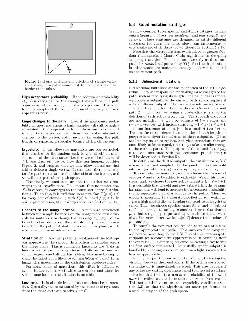
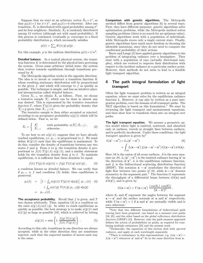
Figure 2: If only additions and deletions of a single vertexare allowed, then paths cannot mutate from one side of thebarrier to the other.

High acceptance probability. If the acceptance probabilitya(y | x) is very small on the average, there will be long pathsequences of the form x, x, . . ., x due to rejections. This leadsto many samples at the same point on the image plane, andappears as noise.

Large changes to the path. Even if the acceptance proba-bility for most mutations is high, samples will still be highlycorrelated if the proposed path mutations are too small. Itis important to propose mutations that make substantialchanges to the current path, such as increasing the pathlength, or replacing a specular bounce with a diffuse one.

Ergodicity. If the allowable mutations are too restricted,it is possible for the random walk to get “stuck” in somesubregion of the path space (i.e. one where the integral off is less than b). To see how this can happen, considerFigure 2, and suppose that we only allow mutations thatadd or delete a single vertex. In this case, there is no wayfor the path to mutate to the other side of the barrier, andwe will miss part of the path space.

Technically, we want to ensure that the random walk con-verges to an ergodic state. This means that no matter howX0 is chosen, it converges to the same stationary distribu-tion p. To do this, it is sufficient to ensure that T (y | x) > 0for every pair of states x, y with f(x) > 0 and f(y) > 0. Inour implementation, this is always true (see Section 5.3.1).

Changes to the image location. To minimize correlationbetween the sample locations on the image plane, it is desir-able for mutations to change the lens edge xk−1xk. Muta-tions to other portions of the path do not provide informa-tion about the path distribution over the image plane, whichis what we are most interested in.

Stratification. Another potential weakness of the Metrop-olis approach is the random distribution of samples acrossthe image plane. This is commonly known as the “balls inbins” effect: if we randomly throw n balls into n bins, wecannot expect one ball per bin. (Many bins may be empty,while the fullest bin is likely to contain Θ(log n) balls.) In animage, this unevenness in the distribution produces noise.

For some kinds of mutations, this effect is difficult toavoid. However, it is worthwhile to consider mutations forwhich some form of stratification is possible.

Low cost. It is also desirable that mutations be inexpen-sive. Generally, this is measured by the number of rays cast,since the other costs are relatively small.

5.3 Good mutation strategies

We now consider three specific mutation strategies, namelybidirectional mutations, perturbations, and lens subpath mu-tations. These strategies are designed to satisfy differentsubsets of the goals mentioned above; our implementationuses a mixture of all three (as we discuss in Section 5.3.4).

Note that the Metropolis framework allows us greater free-dom than standard Monte Carlo algorithms in designingsampling strategies. This is because we only need to com-pute the conditional probability T (y | x) of each mutation:in other words, the mutation strategy is allowed to dependon the current path.

5.3.1 Bidirectional mutations

Bidirectional mutations are the foundation of the MLT algo-rithm. They are responsible for making large changes to thepath, such as modifying its length. The basic idea is simple:we choose a subpath of the current path x, and replace itwith a different subpath. We divide this into several steps.

First, the subpath to delete is chosen. Given the currentpath x = x0 . . .xk, we assign a probability pd[s, t] to thedeletion of each subpath xs . . .xt. The subpath endpointsare not included, i.e. xs . . .xt consists of t − s edges andt− s−1 vertices, with indices satisfying −1 ≤ s < t ≤ k+ 1.

In our implementation, pd[s, t] is a product two factors.The first factor pd,1 depends only on the subpath length; itspurpose is to favor the deletion of short subpaths. (Theseare less expensive to replace, and yield mutations that aremore likely to be accepted, since they make a smaller changeto the current path). The purpose of the second factor pd,2

is to avoid mutations with low acceptance probabilities; itwill be described in Section 5.4.

To determine the deleted subpath, the distribution pd[s, t]is normalized and sampled. At this point, x has been splitinto two (possibly empty) pieces x0 . . .xs and xt . . .xk.

To complete the mutation, we first choose the number ofvertices s′ and t′ to be added to each side. We do this in twosteps: first, we choose the new subpath length, la =s′+t′+1.It is desirable that the old and new subpath lengths be simi-lar, since this will tend to increase the acceptance probability(i.e. it represents a smaller change to the path). Thus, wechoose la according to a discrete distribution pa,1 which as-signs a high probability to keeping the total path length thesame. Then, we choose specific values for s′ and t′ (subjectto s′+ t′+ 1= la), according to another discrete distributionpa,2 that assigns equal probability to each candidate valueof s′. For convenience, we let pa[s′, t′] denote the product ofpa,1 and pa,2.

To sample the new vertices, we add them one at a timeto the appropriate subpath. This involves first samplinga direction according to the BSDF at the current subpathendpoint (or a convenient approximation, if sampling fromthe exact BSDF is difficult), followed by casting a ray to findthe first surface intersected. An initially empty subpath ishandled by choosing a random point on a light source or thelens as appropriate.

Finally, we join the new subpaths together, by testing thevisibility between their endpoints. If the path is obstructed,the mutation is immediately rejected. This also happens ifany of the ray casting operations failed to intersect a surface.

Notice that there is a non-zero probability of throwingaway the entire path, and generating a new one from scratch.This automatically ensures the ergodicity condition (Sec-tion 5.2), so that the algorithm can never get “stuck” ina small subregion of the path space.

Parameter values. The following values have provided rea-sonable results on our test cases. For the probability pd,1[ld]of deleting a subpath of length ld = t−s, we use pd,1[1]=0.25,pd,1[2]=0.5, and pd,1[ld]=2−l for ld ≥ 3. For the probabilitypa,1[la] of adding a subpath of length la, we use pa,1[ld]=0.5,pa,1[ld − 1]=0.15, and pa,1[ld + 1]=0.15, with the remainingprobability assigned to the other allowable subpath lengths.

Evaluation of the acceptance probability. Observe thata(y | x) can be written as the ratio

a(y | x) =R(y | x)

R(x | y), where R(y | x) =

f(y)

T (y | x). (13)

The form of R(y | x) is very similar to the sample valuef(y)/p(y) that is computed by standard Monte Carlo algo-rithms; we have simply replaced an absolute probability p(y)by a conditional probability T (y | x).

Specifically, T (y | x) is the product of the discrete proba-bility pd[s, t] for deleting the subpath xs . . .xt, and the prob-ability density for generating the s′+t′ new vertices of y. Tocalculate the latter, we must take into account all s′+ t′+ 1ways that the new vertices can be split between subpathsgenerated from xs and xt. (Although these vertices weregenerated by a particular choice of s′, the probability T (y | x)must take into account all ways of going from state x to y.)

Note that the unchanged portions of x do not contributeto the calculation of T (y | x). It is also convenient to ignorethe factors of f(x) and f(y) that are shared between thepaths, since this does not change the result.

An example. Let x be a path x0x1x2x3, and suppose thatthe random mutation step has deleted the edge x1x2. It isreplaced by new vertex z0 by casting a ray from x1, so thatthe new path is y = x0x1z0x2x3. (This corresponds to therandom choices s=1, t=2, s′=1, t′=0.)

Let ps(x0→ x1→ z0) be the probability density of sam-pling the direction from x1 to z0, measured with respectto projected solid angle.12 Then the probability density ofsampling z0 (measured with respect to surface area) is givenby ps(x0→x1→z0)G(x1↔z0).

We now have all of the information necessary to computeR(y | x). From (8), the numerator f(y) is

fs(x0,x1, z0)G(x1, z0) fs(x1, z0,x2)G(z0,x2) fs(z0,x2,x3) ,

where the factors shared between R(y | x) and R(x | y) havebeen omitted (and we have dropped the arrow notation forbrevity). The denominator T (y | x) is

pd[1, 2]

[pa[1, 0] ps(x0,x1, z0)G(x1, z0)+ pa[0, 1] ps(x3,x2, z0)G(x2, z0)

].

In a similar way, we find that R(x | y) is given by

fs(x0,x1,x2)G(x1,x2) fs(x1,x2,x3) / pd[1, 3] pa[0, 0] ,where pd and pa now refer to y. To implement this calcula-tion in general, it is convenient to define functions

C(x0,x1,x2,x3) = fs(x0,x1,x2)G(x1,x2) fs(x1,x2,x3)

S(x0,x1,x2) = fs(x0,x1,x2)/ps(x0,x1,x2) , (14)

and then express 1/R(y | x) in terms of these functions. Thisformulation extends easily to subpaths of arbitrary length,and can be evaluated efficiently by precomputing C and Sfor each edge. In this form, it is also easy to handle specularBSDF’s, since the ratio S is always well-defined.

12If p′s(x0→ x1 → z0) is the density with respect to ordinarysolid angle, then ps = p′s/| cos(θo)|, where θo is the angle betweenx1→z0 and the surface normal at x1.

Lens perturbation Caustic perturbation

Figure 3: The lens edge can be perturbed by regenerating itfrom either side: we call these lens perturbations and causticperturbations.

5.3.2 Perturbations

There are some lighting situations where bidirectional mu-tations will almost always be rejected. This happens whenthere are small regions of the path space in which pathscontribute much more than average. This can be caused bycaustics, difficult visibility (e.g. a small hole), or by concavecorners where two surfaces meet (a form of singularity in theintegrand). The problem is that bidirectional mutations arerelatively large, and so they usually attempt to mutate thepath outside the high-contribution region.

One way to increase the acceptance probability is to usesmaller mutations. The principle is that nearby paths willmake similar contributions to the image, and so the accep-tance probability will be high. Thus, rather than havingmany rejections on the same path, we can explore the othernearby paths of the high-contribution region.

Our solution is to choose a subpath of the current path,and move the vertices slightly. We call this type of mutationa perturbation. While the idea can be applied to arbitrarysubpaths, our main interest is in perturbations that includethe lens edge xk−1xk (since other changes do not help toprevent long sample sequences at the same image point). Wehave implemented two specific kinds of perturbations thatchange the lens edge, termed lens perturbations and causticperturbations (see Figure 3). These are described below.

Lens perturbations. We delete a subpath xt . . .xk of theform (L|D)DS∗E (where we have used Heckbert’s regularexpression notation [8]; S, D, E, and L stand for specular,non-specular, lens, and light vertices respectively). This iscalled the lens subpath, and consists of k−t edges and k−t−1vertices. (Note that if xt were specular, then any perturba-tion of xt−1 would result in a path y for which f(y) = 0.)

To replace the lens subpath, we perturb the old imagelocation by moving it a random distance R in a randomdirection φ. The angle φ is chosen uniformly, while R isexponentially distributed between two values r1 < r2:

R = r2 exp(− ln(r2/r1) U) , (15)

where U is uniformly distributed on [0, 1].We then cast a ray at the new image location, and extend

the subpath through additional specular bounces to be thesame length as the original. The mode of scattering at eachspecular bounce is preserved (i.e. specular reflection or trans-mission), rather than making new random choices.13 Thisallows us to efficiently sample rare combinations of events,e.g. specular reflection from a surface where 99% of the lightis transmitted.

The calculation of a(y | x) is similar to the bidirectionalcase. The main difference is the method used for directionalsampling (i.e. distribution (15) instead of the BSDF).

13If the perturbation moves a vertex from a specular to a non-specular material, then the mutation is immediately rejected.

Figure 4: Using a two-chain perturbation to sample causticsin a pool of water. First, the lens edge is perturbed to generatea point x′ on the pool bottom. Then, the direction fromoriginal point x toward the light source is perturbed, and aray is cast from x′ in this direction.

Caustic perturbations. Lens perturbations are not possiblein some situations; the most notable example occurs whencomputing caustics. These paths have the form LS+DE,which is unacceptable for lens perturbations.

However, there is another way to perturb paths with asuffix xt . . .xk of the form (D|L)S∗DE. To do this, we gen-erate a new subpath starting from xt. The direction of thesegment xt→xt+1 is perturbed by an amount (θ, φ), where θis exponentially distributed and φ is uniform. The techniqueis otherwise similar to lens perturbations.

Multi-chain perturbations. Neither of the above can han-dle paths with a suffix of the form (D|L)DS∗DS∗DE, i.e.caustics seen through a specular surface (see Figure 4). Thiscan be handled by perturbing the path through more thanone specular chain. At each non-specular vertex, we choosea new direction by perturbing the corresponding directionof the original subpath.

Parameter values. For lens perturbations, the image reso-lution is a guide to the useful range of values. We use r1 =0.1pixels, while r2 is chosen such that the perturbation regionis 5% of the image area. For caustic and multi-chain per-turbations, we use θ1 = 0.0001 radians and θ2 = 0.1 radians.The algorithm is not particularly sensitive to these values.

5.3.3 Lens subpath mutations

We now describe lens subpath mutations, whose goal is tostratify the samples over the image plane, and also to reducethe cost of sampling by re-using subpaths. Each mutationconsists of deleting the lens subpath of the current path, andreplacing it with a new one. (As before, the lens subpathhas the form (L|D)S∗E.) The lens subpaths are stratifiedacross the image plane, such that every pixel receives thesame number of proposed lens subpath mutations.

We briefly describe how to do this. We initialize the algo-rithm with n′ independent seed paths (Section 5.1), whichare mutated in a rotating sequence. At all times, we alsostore a current lens subpath xe. An eye subpath mutationconsists of deleting the lens subpath of the current path x,and replacing it with xe.

The current subpath xe is re-used a fixed number of timesne, and then a new one is generated. We chose n′ ne,to prevent the same lens subpath from being used multipletimes on the same path.

To generate xe, we cast a ray through a point on theimage plane, and follow zero or more specular bounces untilwe obtain a non-specular vertex.14 To stratify the samples

14At a material with specular and non-specular components, werandomly choose between them.

on the image plane, we maintain a tally of the number oflens subpaths that have been generated at each pixel. Whengenerating a new subpath, we choose a random pixel and, ifit already has its quota of lens subpaths, we choose anotherone. We use a rover to make the search for a non-full pixelefficient. We also control the distribution of samples withineach pixel, by computing a Poisson minimum-disc patternand tiling it over the image plane.

The probability a(y | x) is similar to the bidirectional case,except that there is only one way of generating the new sub-path. (Subpath re-use does not influence the calculation.)

5.3.4 Selecting between mutation types

At each step, we assign a probability to each of the threemutation types. This discrete distribution is sampled to de-termine which kind of mutation is applied to the currentpath.

We have found that it is important to make the prob-abilities relatively balanced. This is because the mutationtypes are designed to satisfy different goals, and it is difficultto predict in advance which types will be the most success-ful. The overall goal is to make mutations that are as largeas possible, while still having a reasonable chance of accep-tance. This can be achieved by randomly choosing betweenmutations of different sizes, so that there is a good chanceof trying an appropriate mutation for any given path.

These observation are similar to those of multiple impor-tance sampling (an alternative name for the technique in[25]). We would like a set of mutations that cover all thepossibilities, even though we may not (and need not) knowthe optimum way to choose among them for a given path.It is perfectly fine to include mutations that are designed forspecial situations, and that result in rejections most of thetime. This increases the cost of sampling by only a smallamount, and yet it can increase robustness considerably.

5.4 Refinements

We describe several ideas that improve the efficiency of MLT.

Direct lighting. We use standard techniques for directlighting (e.g. see [21]), rather than the Metropolis algorithm.In most cases, these standard methods give better results atlower cost, due to the fact that the Metropolis samples arenot as well-stratified across the image plane (Section 5.2).By excluding direct lighting paths from the Metropolis cal-culation, we can apply more effort to the indirect lighting.

Using the expected sample value. For each proposed muta-tion, there is a probability a(y | x) of accumulating an imagesample at y, and a probability 1 − a(y | x) of accumulatinga sample at x. We can make this more efficient by alwaysaccumulating a sample at both locations, weighted by thecorresponding probability. Effectively, we have replaced arandom variable by its expected value (a common variancereduction technique [11]). This is especially useful for sam-pling the dim regions of the image, which would otherwisereceive very few samples.

Importance sampling for mutation probabilities. We de-scribe a technique that can increase the efficiency of MLTsubstantially, by increasing the average acceptance proba-bility. The idea is to implement a form of importance sam-pling which with respect to a(y | x), when deciding whichmutation to attempt. This is done by weighting each pos-sible mutation according to the probability with which the

(a) Bidirectional path tracing with 40 samples per pixel.

(b) Metropolis light transport with an average of 250 mutations per pixel [the same computation time as (a)].

Figure 5: All of the light in the visible portion of this scene comes through a door that is slightly ajar, such that about 0.1%of the light in the adjacent room comes through the doorway. The light source is a diffuse ceiling panel at the far end of a largeadjacent room, so that virtually all of the light coming through the doorway has bounced several times. The MLT algorithm efficientlygenerates paths that go through the small opening between the rooms, by always preserving a path segment that goes through thedoorway. The images are 900 by 500 pixels, and include the effects of all paths up to length 10.

deleted subpath can be regenerated. (This is the factor pd,2

mentioned in Section 5.3.1.)

Let x be the current path, and consider a mutation thatdeletes the subpath xs . . .xt. The insight is that given onlythe deleted subpath, it is already possible to compute someof the factors in the acceptance probability a(y | x). In par-ticular, from (13) we see that a(y | x) is proportional to1 /R(x | y), and that it is possible to compute all the com-

ponents of R(x | y) except for the discrete probabilities pd

and pa (these apply to y, which has not been generated yet).The computable factors of 1 /R(x | y) are denoted pd,2. Inthe example of Section 5.3.1, for instance, we have

pd,2[1, 2] = 1/C(x0,x1,x2,x3) .

The discrete probabilities for each mutation type areweighted by this factor, before a mutation is selected.

6 Results

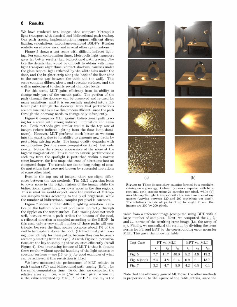
We have rendered test images that compare Metropolislight transport with classical and bidirectional path tracing.Our path tracing implementations support efficient directlighting calculations, importance-sampled BSDF’s, Russianroulette on shadow rays, and several other optimizations.

Figure 5 shows a test scene with difficult indirect light-ing. For equal computation times, Metropolis light transportgives far better results than bidirectional path tracing. No-tice the details that would be difficult to obtain with manylight transport algorithms: contact shadows, caustics underthe glass teapot, light reflected by the white tiles under thedoor, and the brighter strip along the back of the floor (dueto the narrow gap between the table and the wall). Thisscene contains diffuse, glossy, and specular surfaces, and thewall is untextured to clearly reveal the noise levels.

For this scene, MLT gains efficiency from its ability tochange only part of the current path. The portion of thepath through the doorway can be preserved and re-used formany mutations, until it is successfully mutated into a dif-ferent path through the doorway. Note that perturbationsare not essential to make this process efficient, since the paththrough the doorway needs to change only infrequently.

Figure 6 compares MLT against bidirectional path trac-ing for a scene with strong indirect illumination and caus-tics. Both methods give similar results in the top row ofimages (where indirect lighting from the floor lamp domi-nates). However, MLT performs much better as we zoominto the caustic, due to its ability to generate new paths byperturbing existing paths. The image quality degrades withmagnification (for the same computation time), but onlyslowly. Notice the streaky appearance of the noise at thehighest magnification. This is due to caustic perturbations:each ray from the spotlight is perturbed within a narrowcone; however, the lens maps this cone of directions into anelongated shape. The streaks are due to long strings of caus-tic mutations that were not broken by successful mutationsof some other kind.

Even in the top row of images, there are slight differ-ences between the two methods. The MLT algorithm leadsto lower noise in the bright regions of the image, while thebidirectional algorithm gives lower noise in the dim regions.This is what we would expect, since the number of Metrop-olis samples varies according to the pixel brightness, whilethe number of bidirectional samples per pixel is constant.

Figure 7 shows another difficult lighting situation: caus-tics on the bottom of a small pool, seen indirectly throughthe ripples on the water surface. Path tracing does not workwell, because when a path strikes the bottom of the pool,a reflected direction is sampled according to the BRDF. Inthis case, only a very small number of those paths will con-tribute, because the light source occupies about 1% of thevisible hemisphere above the pool. (Bidirectional path trac-ing does not help for these paths, because they can be gener-ated only starting from the eye.) As with Figure 6, perturba-tions are the key to sampling these caustics efficiently (recallFigure 4). One interesting feature of MLT is that it obtainsthese results without special handling of the light sources orspecular surfaces — see [16] or [3] for good examples of whatcan be achieved if this restriction is lifted.

We have measured the performance of MLT relative topath tracing (PT) and bidirectional path tracing (BPT), forthe same computation time. To do this, we computed therelative error ej = (mj −mj)/mj at each pixel, where mj

is the value computed by MLT, PT, or BPT, and mj is the

(a) (b)

Figure 6: These images show caustics formed by a spotlightshining on a glass egg. Column (a) was computed with bidi-rectional path tracing using 25 samples per pixel, while (b)uses Metropolis light transport with the same number of rayqueries (varying between 120 and 200 mutations per pixel).The solutions include all paths of up to length 7, and theimages are 200 by 200 pixels.

value from a reference image (computed using BPT with alarge number of samples). Next, we computed the l1, l2,and l∞ norms of the resulting error image (i.e. the array ofej). Finally, we normalized the results, by dividing the errornorms for PT and BPT by the corresponding error norm forMLT. This gave the following table:

Test Case PT vs. MLT BPT vs. MLT

l1 l2 l∞ l1 l2 l∞

Fig. 5 7.7 11.7 40.0 5.2 4.9 13.2

Fig. 6 (top) 2.4 4.8 21.4 0.9 2.1 13.7

Fig. 7 3.2 4.7 5.0 4.2 6.5 6.1

Note that the efficiency gain of MLT over the other methodsis proportional to the square of the table entries, since the

(a) Path tracing with 210 samples per pixel.

(b) Metropolis light transport with an average of 100 mutations per pixel [the same computation time as (a)].

Figure 7: Caustics in a pool of water, viewed indirectly through the ripples on the surface. It is difficult for unbiased Monte Carloalgorithms to find the important transport paths, since they must be generated starting from the lens, and the light source onlyoccupies about 1% of the hemisphere as seen from the pool bottom (which is curved). The MLT algorithm is able to sample thesepaths efficiently by means of perturbations. The images are 800 by 500 pixels.

error for PT and BPT decreases according to the square rootof the number of samples. For example, the RMS relativeerror in Figure 5(a) is 4.9 times higher than in Figure 5(b),and so approximately 25 times more BPT samples wouldbe required to achieve the same error levels. Even in thetopmost images of Figure 6 (for which BPT is well-suited),notice that MLT and BPT are competitive.

The computation times were approximately 15 minutesfor each image in Figure 6, 2.5 hours for the images in Fig-

ure 7, and 4 hours for the images in Figure 5 (all times mea-sured on a 190 MHz MIPS R10000 processor). The memoryrequirements are modest: we only store the scene model,the current image, and a single path (or a small number ofpaths, if the mutation technique in Section 5.3.3 is used).For high-resolution images, the memory requirements couldbe reduced further by collecting the samples in batches, sort-ing them in scanline order, and applying them to an imageon disk.

7 Conclusions

We have presented a novel approach to global illuminationproblems, by showing how to adapt the Metropolis samplingmethod to light transport. Our algorithm starts from a fewseed light transport paths and applies a sequence of ran-dom mutations to them. In the steady state, the resultingMarkov chain visits each path with a probability propor-tional to that path’s contribution to the image. The MLTalgorithm is notable for its generality and simplicity. A sin-gle control structure can be used with different mutationstrategies to handle a variety of difficult lighting situations.In addition, the MLT algorithm has low memory require-ments and always computes an unbiased result.

Many refinements of this basic idea are possible. For ex-ample, with modest changes we could use MLT to computeview-independent radiance solutions, by letting the mj bethe basis function coefficients, and defining f(x) =

∑jfj(x).

We could also use MLT to render a sequences of images (asin animation), by sampling the the entire space-time of pathsat once (thus, a mutation might try to perturb a path for-ward or backward in time). Another interesting problem isto determine the optimal settings for the various parametersused by the algorithm. The values we use have not been ex-tensively tuned, so that further efficiency improvements maybe possible. We hope to address some of these refinementsand extensions in the future.

8 Acknowledgements

We would especially like to thank the anonymous reviewersfor their detailed comments. In particular, review #4 led tosignificant improvements in the formulation and expositionof the paper. Thanks also to Matt Pharr for his commentsand artwork.

This research was supported by NSF contract numberCCR-9623851, and MURI contract DAAH04-96-1-0007.

References

[1] Arvo, J., and Kirk, D. Particle transport and image syn-thesis. Computer Graphics (SIGGRAPH 90 Proceedings)24, 4 (Aug. 1990), 63–66.

[2] Beyer, M., and Lange, B. Rayvolution: An evolutionaryray tracing algorithm. In Eurographics Rendering Workshop1994 Proceedings (June 1994), pp. 137–146. Also in Photo-realistic Rendering Techniques, Springer-Verlag, New York,1995.

[3] Collins, S. Reconstruction of indirect illumination fromarea luminaires. In Rendering Techniques ’95 (1995),pp. 274–283. Also in Eurographics Rendering Workshop 1996Proceedings (June 1996).

[4] Cook, R. L., Porter, T., and Carpenter, L. Distributedray tracing. Computer Graphics (SIGGRAPH 84 Proceed-ings) 18, 3 (July 1984), 137–145.

[5] Dutre, P., and Willems, Y. D. Potential-driven MonteCarlo particle tracing for diffuse environments with adaptiveprobability density functions. In Rendering Techniques ’95(1995), pp. 306–315. Also in Eurographics Rendering Work-shop 1996 Proceedings (June 1996).

[6] Goldberg, D. E. Genetic Algorithms in Search, Optimiza-tion, and Machine Learning. Addison-Wesley, Reading, Mas-sachusetts, 1989.

[7] Halmos, P. R. Measure Theory. Van Nostrand, New York,1950.

[8] Heckbert, P. S. Adaptive radiosity textures for bidirec-tional ray tracing. In Computer Graphics (SIGGRAPH 90Proceedings) (Aug. 1990), vol. 24, pp. 145–154.

[9] Jensen, H. W. Importance driven path tracing using thephoton map. In Eurographics Rendering Workshop 1995(June 1995), Eurographics.

[10] Kajiya, J. T. The rendering equation. In ComputerGraphics (SIGGRAPH 86 Proceedings) (Aug. 1986), vol. 20,pp. 143–150.

[11] Kalos, M. H., and Whitlock, P. A. Monte Carlo Methods,Volume I: Basics. John Wiley & Sons, New York, 1986.

[12] Lafortune, E. P., and Willems, Y. D. Bi-directional pathtracing. In CompuGraphics Proceedings (Alvor, Portugal,Dec. 1993), pp. 145–153.

[13] Lafortune, E. P., and Willems, Y. D. A theoretical frame-work for physically based rendering. Computer Graphics Fo-rum 13, 2 (June 1994), 97–107.

[14] Lafortune, E. P., and Willems, Y. D. A 5D tree to re-duce the variance of Monte Carlo ray tracing. In RenderingTechniques ’95 (1995), pp. 11–20. Also in Eurographics Ren-dering Workshop 1996 Proceedings (June 1996).

[15] Metropolis, N., Rosenbluth, A. W., Rosenbluth, M. N.,

Teller, A. H., and Teller, E. Equations of state calcu-lations by fast computing machines. Journal of ChemicalPhysics 21 (1953), 1087–1091.

[16] Mitchell, D. P., and Hanrahan, P. Illumination fromcurved reflectors. In Computer Graphics (SIGGRAPH 92Proceedings) (July 1992), vol. 26, pp. 283–291.

[17] Pattanaik, S. N., and Mudur, S. P. Adjoint equations andrandom walks for illumination computation. ACM Transac-tions on Graphics 14 (Jan. 1995), 77–102.

[18] Peskun, P. H. Optimum monte-carlo sampling using markovchains. Biometrika 60, 3 (1973), 607–612.

[19] Reif, J. H., Tygar, J. D., and Yoshida, A. Computabilityand complexity of ray tracing. Discrete and ComputationalGeometry 11 (1994), 265–287.

[20] Shirley, P., Wade, B., Hubbard, P. M., Zareski, D.,

Walter, B., and Greenberg, D. P. Global illuminationvia density-estimation. In Eurographics Rendering Work-shop 1995 Proceedings (June 1995), pp. 219–230. Also inRendering Techniques ’95, Springer-Verlag, New York, 1995.

[21] Shirley, P., Wang, C., and Zimmerman, K. Monte Carlomethods for direct lighting calculations. ACM Transactionson Graphics 15, 1 (Jan. 1996), 1–36.

[22] Spanier, J., and Gelbard, E. M. Monte Carlo Principlesand Neutron Transport Problems. Addison-Wesley, Reading,Massachusetts, 1969.

[23] Veach, E. Non–symmetric scattering in light transport al-gorithms. In Eurographics Rendering Workshop 1996 Pro-ceedings (June 1996). Also in Rendering Techniques ’96,Springer-Verlag, New York, 1996.

[24] Veach, E., and Guibas, L. Bidirectional estimators forlight transport. In Eurographics Rendering Workshop 1994Proceedings (June 1994), pp. 147–162. Also in PhotorealisticRendering Techniques, Springer-Verlag, New York, 1995.

[25] Veach, E., and Guibas, L. J. Optimally combining sam-pling techniques for Monte Carlo rendering. In SIGGRAPH95 Proceedings (Aug. 1995), Addison-Wesley, pp. 419–428.

[26] Whitted, T. An improved illumination model for shadeddisplay. Communications of the ACM 32, 6 (June 1980),343–349.

Appendix A

To prove that (12) is unbiased, we show that the following identityis satisfied at each step of the random walk:∫

IRw qi(w, x) dw = f(x) , (16)

where qi is the joint probability distribution of the i-th weightedsample (Wi, Xi). Clearly this condition is satisfied by q0, notingthat q0(w, x) = δ(w − f(x)/p0(x)) p0(x) (where δ denotes theDirac delta distribution).

Next, observe that (4) is still true with pj replaced by qj(w, x)(since the mutations set Wi = Wi−1). Multiplying both sides of(4) by w and integrating, we obtain∫

IRw qi(w, x) dw =

∫IRw qi−1(w, x) ,

so that (16) is preserved by each mutation step.Now given (16), the desired estimate (12) is unbiased since

E[Wi wj(Xi)] =∫

Ω

∫IRw wj(x) pi(w, x) dw dµ(x)

=∫

Ωwj(x) f(x) dµ(x) = mj .