Metropolis Light Transport for ParticipatingMedia

Mark Pauly Thomas Kollig Alexander KellerETH Zurich University of Kaiserslautern

pauly@inf.ethz.ch kollig, keller@informatik.uni-kl.de

Abstract. In this paper we show how Metropolis Light Transport can be ex-tended both in the underlying theoretical framework and the algorithmic imple-mentation to incorporate volumetric scattering. We present a generalization of thepath integral formulation that handles anisotropic scattering in non-homogeneousmedia. Based on this framework we introduce a new mutation strategy thatis specifically designed for participating media. Our algorithm includes effectssuch as volume caustics and multiple volume scattering, is not restricted to cer-tain classes of geometry and scattering models and has minimal memory require-ments. Furthermore, it is unbiased and robust, in the sense that it produces sat-isfactory results for a wide range of input scenes and lighting situations withinacceptable time bounds.

1 Introduction

Many global illumination algorithms have been developed for solving the light transportproblem, yet the majority of these methods focuses on scenes without participatingmedia. Volumetric effects due to clouds, fog, smoke or fire can greatly enhance therealism of a rendered image, however, and in many applications are the decisive factorof the simulation. Visibility analysis for traffic or building design, fire research, flightsimulation, and high-quality special effects in animation systems all rely on a realisticdepiction of volumetric phenomena [Rus94].

Global illumination algorithms for participating media can be classified accordingto the directional behavior (isotropic/anisotropic, single/multiple scattering) and spatialvariation (homogeneous/inhomogeneous) of the supported media. Finite element meth-ods for isotropic scattering include zonal methods [RT87] and other extensions to theclassical radiosity approach, such as hierarchical radiosity [Sil95, Bha93]. Anisotropicscattering was modeled deterministically using spherical harmonics[KVH84], discrete ordinates [LBC94] and point collocation [BT92]. All these algo-rithms require some discretization of the volume or the directional space into finite el-ements and compute the interactions between these elements. Thus excessive amountsof memory are required to effectively capture sharp discontinuities of the illumination(e.g. caustics) or uneven directional distributions (e.g. glossy reflections).

Monte Carlo methods are a promising alternative and have been used extensively inglobal illumination. In the context of participating media, various extensions to existingMonte Carlo approaches have been proposed. Pattanaik and Mudur [PM93] presented aMonte Carlo light tracing algorithm that generates random walks starting from the lightsources. They sample interaction points in the volume according to the transmittanceof the medium. Lafortune and Willems [LW96] improved on this approach by creat-ing paths both from the light sources and the eye and combining all valid connections

1

between these paths in a multiple sample estimate [VG95]. This led to a bidirectionalpath tracing algorithm for non-emitting media. A two-pass algorithm based on pho-ton density estimation was presented by Jensen and Christensen in [JC98]. Althoughsimple and efficient the method suffers from various artifacts (e.g. blurred shadow andcaustic borders) and requires substantial amounts of memory for difficult lighting sit-uations. In [VG97] a new global illumination algorithm was proposed, the Metropolislight transport (MLT) algorithm. This first application of the Metropolis sampling tech-nique [MRR+53] to the field of computer graphics resulted in a versatile Monte Carlomethod for image synthesis.

In this paper we show how the MLT algorithm can be extended to include volumetricscattering. Section2 briefly reviews the fundamental equation governing the equilib-rium distribution of light in scenes with participating media. In section3 we extendthe path integral framework and show how it can be applied to solve the light trans-port problem. Section4 is concerned with different aspects of sampling and presentsan improved ray marching algorithm. Rendering with the Metropolis light transportalgorithm is described in section5, where we introduce a new mutation strategy forparticipating media. We present our results in section6 and draw the conclusions in thefinal section.

2 Light Transport for Participating Media

We consider the radiance distribution in a finite volumeV ⊂ R3. ∂V is the boundaryof V, i.e. a finite set of surfaces describing the objects of the scene. The space betweenobjects is denoted byV0 := V \∂V, and can be filled with participating media. Accord-ing to the theory of radiative transfer [Cha50], the equilibrium distribution of radianceL in V0 is given by theglobal balance equation

ω · ∇L(x, ω) = Le,V0(x, ω) + σs(x)∫S2

fp(ω, x, ω′)L(x, ω′) dω′

−σa(x)L(x, ω)− σs(x)L(x, ω). (1)

It describes the spatial variation of radiance due to emission, in-scattering, absorptionand out-scattering.Le,V0 is the volume emittance function that defines volumetric lightsources such as fire or plasma.S2 is the unit sphere of all directions,σs andσa arethe scattering and absorption coefficients, respectively, andfp is the phase function,which describes the scattering characteristics of the medium. Iffp is independent ofdirection, we have isotropic scattering, which is analogous to perfectly diffuse reflectionon surfaces. Ifσa andσs are independent of position, we have a homogeneous medium.To obtain a complete description ofL in V we need to specify the boundary conditionsfor x ∈ ∂V, given by thelocal scattering equation

L(x, ω) = Le,∂V(x, ω) +∫S2

fs(ω, x, ω′)L(x, ω′) cos Θx dω′, (2)

wherefs is the bidirectional scattering distribution function (BSDF),Θx is the anglebetweenω′ and the surface normal inx, andLe,∂V defines the emittance on surfaces.We now derive the Fredholm integral equation of the second kind, describing the lighttransport in the presence of participating media. The resulting integral equation willbe solved using the Neumann series. Incorporating the boundary conditions (2) into

2

equation (1) [Arv93] yields the integral equation

L(x, ω) = τ(x∂V , x)L(x∂V , ω) (3)

+∫ x

x∂V

τ(x′, x)[Le,V0(x′, ω) + σs(x′)

∫S2

fp(ω, x′, ω′)L(x′, ω′)dω′]

dx′,

wherex∂V := h(x,−ω) ∈ ∂V is the closest surface point fromx in direction−ωdetermined by the ray casting functionh. Equation (3) expresses radiance as the sumof the exitant radiance atx∂V and the accumulated emitted and in-scattered radiancebetweenx∂V andx. These components are attenuated by the path transmittance

τ(x, x′) := e−∫ x′

xσe(x′′)dx′′ ,

which accounts for absorption and out-scattering with the extinction coefficientσe :=σa + σs. We define theincident surface emittance(with x∂V as above) as

Li,∂V(x, ω) := τ(x∂V , x)Le,∂V(x∂V , ω),

the incident volume emittanceas

Li,V0(x, ω) :=∫ x

x∂V

τ(x′, x)Le,V0(x′, ω)dx′,

thesurface light transport operatoras

(T∂VL)(x, ω) := τ(x, x∂V)∫S2

fs(ω, x∂V , ω′)L(x∂V , ω′) cos Θx∂Vdω′,

and thevolume light transport operatoras

(TV0L)(x, ω) :=∫ x

x∂V

τ(x′, x)σs(x′)∫S2

fp(ω, x′, ω′)L(x′, ω′) dω′dx′.

Using these definitions we can rewrite equation (3) in operator notation as

L = (Li,∂V + Li,V0)︸ ︷︷ ︸=:Li

+(T∂V + TV0)︸ ︷︷ ︸=:T

L,

which clearly exhibits the Fredholm integral equation structure. Given that‖Tα‖ < 1,α ∈ N, which holds for all physically valid scene models where no perfect reflectors ortransmitters exist, the Neumann series can be applied:

L =∞∑

j=0

TjLi =∞∑

j=0

(T∂V + TV0)j(Li,∂V + Li,V0)

= Li,∂V + Li,V0 + T∂VLi,∂V + TV0Li,∂V + · · · (4)

3

light source

x3

x2

mediumsensor

object

x1

x0

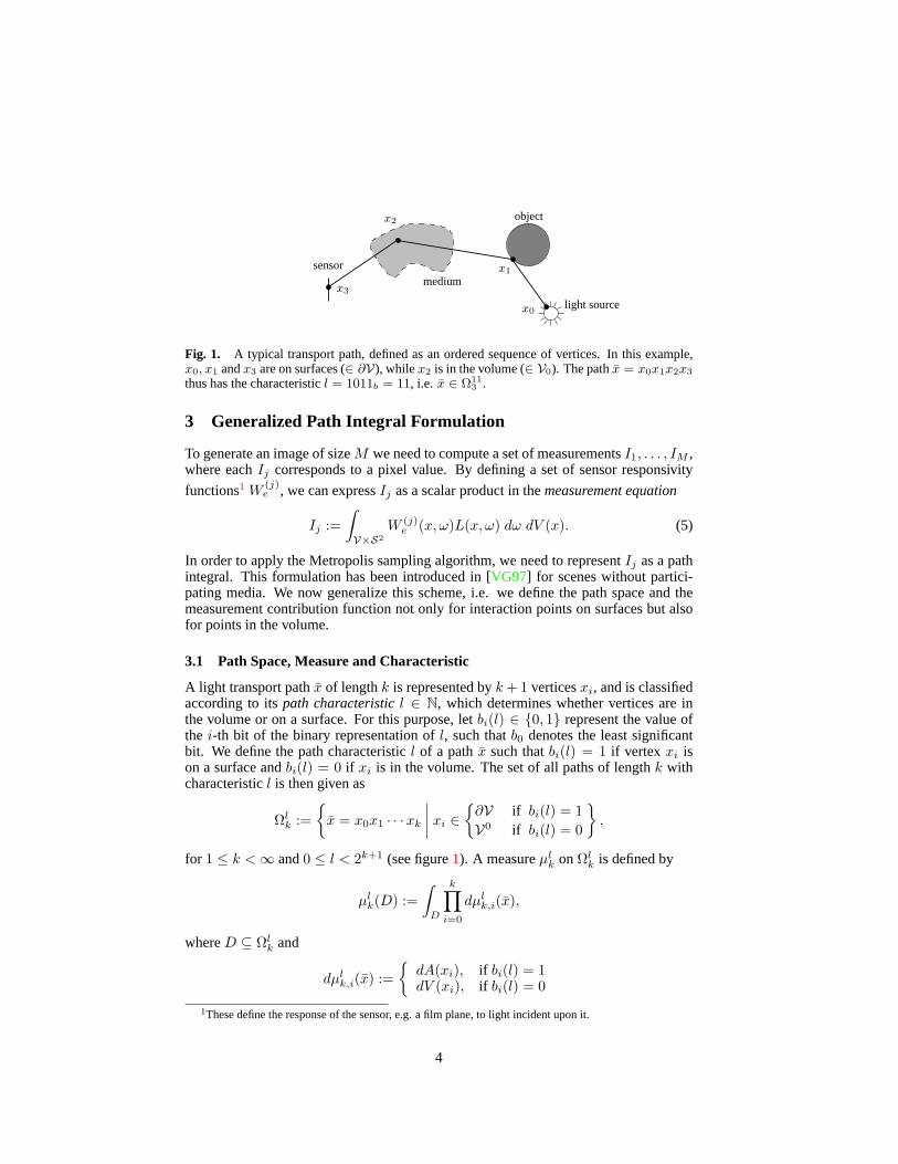
Fig. 1. A typical transport path, defined as an ordered sequence of vertices. In this example,x0, x1 andx3 are on surfaces (∈ ∂V), whilex2 is in the volume (∈ V0). The pathx = x0x1x2x3

thus has the characteristicl = 1011b = 11, i.e. x ∈ Ω113 .

3 Generalized Path Integral Formulation

To generate an image of sizeM we need to compute a set of measurementsI1, . . . , IM ,where eachIj corresponds to a pixel value. By defining a set of sensor responsivity

functions1 W(j)e , we can expressIj as a scalar product in themeasurement equation

Ij :=∫V×S2

W (j)e (x, ω)L(x, ω) dω dV (x). (5)

In order to apply the Metropolis sampling algorithm, we need to representIj as a pathintegral. This formulation has been introduced in [VG97] for scenes without partici-pating media. We now generalize this scheme, i.e. we define the path space and themeasurement contribution function not only for interaction points on surfaces but alsofor points in the volume.

3.1 Path Space, Measure and Characteristic

A light transport pathx of lengthk is represented byk + 1 verticesxi, and is classifiedaccording to itspath characteristicl ∈ N, which determines whether vertices are inthe volume or on a surface. For this purpose, letbi(l) ∈ 0, 1 represent the value ofthe i-th bit of the binary representation ofl, such thatb0 denotes the least significantbit. We define the path characteristicl of a pathx such thatbi(l) = 1 if vertex xi ison a surface andbi(l) = 0 if xi is in the volume. The set of all paths of lengthk withcharacteristicl is then given as

Ωlk :=

x = x0x1 · · ·xk

∣∣∣∣ xi ∈

∂V if bi(l) = 1V0 if bi(l) = 0

,

for 1 ≤ k < ∞ and0 ≤ l < 2k+1 (see figure1). A measureµlk onΩl

k is defined by

µlk(D) :=

∫D

k∏i=0

dµlk,i(x),

whereD ⊆ Ωlk and

dµlk,i(x) :=

dA(xi), if bi(l) = 1dV (xi), if bi(l) = 0

1These define the response of the sensor, e.g. a film plane, to light incident upon it.

4

for a pathx = x0 · · ·xk. Now we can define thepath space

Ω :=∞⋃

k=1

2k+1−1⋃l=0

Ωlk,

as the set of all finite-length paths with the associatedpath space measure

µ(D) :=∞∑

k=1

2k+1−1∑l=0

µlk(D ∩ Ωl

k).

3.2 Measurement Contribution Function

The measurement contribution function can be defined directly in terms of paths andpath vertices by transforming the integration domain of the inner integration of equa-tion (3) from S2 to V. The corresponding conversion of measures is reflected in thegeneralized geometric term2

G(x ↔ y) := V (x ↔ y)Dx(y) ·Dy(x)‖x− y‖2

τ(x ↔ y),

whereDx(y) := |ωxy · n(x)|, if x ∈ ∂V. ωxy is the unit direction vector fromx to yandn(x) the surface normal inx. For x ∈ V0 we setDx(y) equal to one.Dy(x) isdefined symmetrically. The visibility functionV (x ↔ y) is one ifx andy are mutuallyvisible, i.e. if the connecting ray is not blocked by an object, and zero otherwise. Wedefine the measurement contribution function as

fj(x) := Le(x0 → x1)G(x0 ↔ x1) · (6)

·

[k−1∏i=1

(f(xi−1 → xi → xi+1)G(xi ↔ xi+1)

)]·W (j)

e (xk−1 → xk),

wherex = x0 . . . xk,

Le(x → x′) :=

Le,∂V(x → x′) x ∈ ∂VLe,V0(x → x′) x ∈ V0

and

f(x → x′ → x′′) :=

fs(x → x′ → x′′) x′ ∈ ∂Vσs(x′)fp(x → x′ → x′′) x′ ∈ V0 .

Now we can insert the Neumann series (4) into the measurement equation (5), yielding

Ij =∞∑

k=1

2k+1−1∑l=0

∫Ωl

k

fj(x)dµlk(x) =

∫Ω

fj(x)dµ(x). (7)

Each integral overΩlk of the above equation corresponds to exactly one addend of equa-

tion (4). In physical terms,fj describes the differential flux that is transported along apath towards pixelj. Equation (7) defines a measurement as an integral over the infinite-dimensional path space. This allows for a whole new set of integration techniques to beapplied for solving the light transport problem in the presence of participating media.

2We use the common arrow notation for specifying a direction. The↔ symbol indicates symmetry of thearguments.

5

4 Sampling

In order to evaluate the path integral (7) we need to build transport paths with respectto an appropriate probability density function (pdf). We split the generation of pathsinto an alternating sequence of scattering and propagation events: A scattering eventchooses a direction at a given vertexx by sampling according to the phase functionfp

(for x ∈ V0) or the BSDFfs (for x ∈ ∂V). A propagation event determines the nextinteraction pointx′ in a given directionω starting fromx. This is done by samplingthe distanced betweenx andx′ according to the path transmittanceτ . The pdf of thewhole path is then simply the product of all scattering and propagation pdfs, as theseare independent of each other.

4.1 Line Integral Computation

Propagation in the absence of participating media is straightforward, as the new interac-tion point is uniquely determined by the ray casting functionh. If a ray passes througha medium, we generate the next interaction point with the inversion method [HM72],and we obtain an expression for the distanced by normalizing, integrating and invertingτ .

Homogeneous Media. The homogeneous case is simple, because here we have theexplicit expressiond = − ln(1 − ξ)/σe, whereξ is a uniformly distributed randomvariable in[0, 1). All we need to do is compare the sampledd with the distances tothe closest surface pointx∂V . If d < s, we setx′ := x + d · ω, otherwise we choosex′ := x∂V and adapt the probability density accordingly.

Inhomogeneous Media. These require more work, since we need to computed fromthe implicit equationln(1−ξ) =

∫ d

0σe(x+tω)dt. This is done with aray marchingal-

gorithm [PH89], which accumulatesσe along the ray(x, ω) until the thresholdln(1−ξ)is reached or the surface pointx∂V is hit. In effect, a ray marching algorithm approxi-mates a one-dimensional integral by dividing the ray into a number of disjoint segmentsand evaluatingσe at certain points within each segment.Equidistant samplingtraversesthe ray with constant stepsize∆, which produces visible artifacts due to aliasing, asdepicted in figure2 (a). The explanation for the layers in the cloud is simple: Light isemitted downwards from the light source at the ceiling and hits the cloud. As the traver-sal of the cloud data3 starts at the top surface of its cubic bounding box, the interactionsin the medium occur roughly within the same horizontal layers, whose vertical spac-ing is determined by the size of the ray segments∆. Consequently, different transportpaths that contribute to the same pixel are correlated. These effects can be eliminatedby randomly perturbing the sample point within each ray segment, a method knownas jittering. This leads tostratified sampling, a Monte Carlo technique for numericalintegration. While stratified sampling reduces aliasing (see figure2 (b)), it is not a par-ticularly efficient sampling method for this kind of integration problem. Monte Carlointegration is particularly suitable for high-dimensional integrals with discontinuitiesin the integrand. Here we have a one-dimensional, rather smooth continuous function,favoring deterministic approaches. Therefore we have implemented a combination ofequidistant and stratified sampling. Instead of using independent random samples in

3We store inhomogeneous media on a three-dimensional grid with intermediate values being computedthrough tri-linear interpolation.

6

∆

σe(x)

xi = i ·∆ x

ξ1

x

σe(x)

xi = (i + ξi)∆

ξ0 ξξξξ

xi = (i + ξ)∆ x

σe(x)

(a) equidistant (b) stratified (c) random offset

Fig. 2. Different ray marching strategies. The lower picture shows the sampling method, illus-trated for box integration. In the upper row is an image generated with this method. Equidistantsampling clearly reveals aliasing artifacts which are no longer visible in the randomized versionsof the ray marching algorithm.

each ray segment, we choose an initial random offset that is applied to all subsequentsamples of the current ray (see2 (c)). This breaks the correlation of different transportpaths (and hence reduces aliasing) but keeps the integration essentially deterministicand thus more efficient. In general we found an efficiency gain of 30-45% for randomoffset sampling as compared to stratified sampling. Since about 25% of the total com-putation time of figure2 are spent on sampling the medium, this leads to an essentialdecrease in overall rendering time of about 10% for this scene. The samples generatedthis way can be used as input for an adaptive ray marching scheme as used in [JC98].

5 Rendering

In [VG97] Veach and Guibas presented the Metropolis Light Transport (MLT) algo-rithm for scenes in vacuum. We have extended this approach to incorporate participat-ing media, based on the generalized version of the path integral as defined in section3.MLT makes use of theMetropolis sampling algorithm[MRR+53], a very powerfulmethod for the simulation of random variables. The basic idea is to generate a randomwalk x0, x1, . . . through the path spaceΩ and deposit a certain constant amount of en-ergy at each pixel a path passes through. The desired image is obtained by distributingthe paths proportionally to their contribution to the final image. Metropolis samplinggenerates this distribution by first proposing a mutation of the current path and comput-ing the corresponding acceptance probabilityα. Samplingα then determines whetherthe mutated path is accepted or rejected as the next sample of the random walk. Notethat the paths generated this way are correlated, which allows various forms of co-herence to be exploited. On the other hand we are faced with a potential increase invariance as compared to independent sampling.

MLT requires an initialization step which determines the total image brightness andgenerates the seed path for the Markov chain of paths. Similar to [VG97], our initial-

7

ization uses bidirectional path tracing, which we extended to incorporate participatingmedia [LW96]. A more detailed description of Metropolis sampling and its applicationto evaluate the path integral can be found in [Vea97].

5.1 Mutation Strategies

Generating a new mutation and computing the corresponding acceptance probabilityis central to the MLT algorithm. We use a set of different mutation strategies for thispurpose and randomly select one of them to create the proposed mutation.

1. Bidirectional mutationsdelete a contiguous section of the current path and re-place it with a new path section by appending vertices to both ends of the createdsubpaths. Adapting the bidirectional mutation strategy described in [VG97] toour generalized path integral framework is straightforward, so we omit a detaileddiscussion here.

2. Perturbationsexploit the fact that small variations to the path most likely lead tosimilar image contributions and hence a high acceptance probability. We distin-guish two types of perturbations:

(a) Scattering perturbationsdisplace the direction vector at a certain vertex,(b) Propagation perturbationsdisplace the interaction point along a certain ray

segment.

The mutated path is then created by retracing the original path, while preservingthe path characteristic. In a sense, scattering and propagation perturbations arecomplementary. The first perturbs a direction hoping to obtain a similar interac-tion point, while the latter perturbs an interaction point hoping to obtain a similardirection. The idea of both is to sample path space locally. Once an importantpath has been found, neighboring paths are explored as well. This is especiallybeneficial for bright areas of the image, such as caustics. Another important fea-ture of perturbations is that they alter the image location. This leads to a betterdistribution of paths over the image plane and significantly reduces the varianceof the generated images.

We have implemented two scattering perturbations:Sensor perturbationsalter the lo-cation on the image plane4 and retrace the path towards the light source. This mutationstrategy combines the lens and multi-chain perturbations of [VG97]. Caustic perturba-tionsretrace the path towards the eye, after perturbing the direction vector of the secondpath edge from the eye.

Propagation Perturbation. This mutation strategy is specifically designed for partic-ipating media. Letx = x0 . . . xk denote the current transport path, wherex0 is a pointon a light source andxk is a point on the sensor. Similarly,y = y0 . . . yk is the proposedmutation ofx. If xk−1 is an interaction point in the medium, i.e.xk−1 ∈ V0, this vertexis displaced along the line fromxk−2 to xk−1 to obtainyk−1. This new vertex is thenconnected with the eyepoint to determine the new sensor locationyk. xk−1 is moved adistance D in either direction alongxk−2xk−1 according to the pdf

p(D) ∝ 1D

, D ∈ [Dmin, Dmax],

4We use the common pinhole camera model, specified by an eye point and an image plane, such that eachpoint of the image plane corresponds to exactly one pixel of the final image.

8

whereDmin andDmax specify the minimal and maximal distance, respectively (seefigure 3). If yk−1 falls outside the medium, orxk−1 /∈ V0 the mutation is rejected,i.e. its acceptance probability is set to zero. Note that propagation perturbation iscomputationally very cheap as it only requires one occlusion test to check whether theconnection with the eyepoint is unobstructed.

sensoreye light source

Fig. 3. Propagation perturbation. The interaction point is spatially displaced according to theindicated distribution.

6 Simulation Results

We have implemented our version of the MLT algorithm based on the experimental raytracing kernel McRender [Kel98], which supports fast BSP ray intersections and oc-clusion testing. We use a convex combination of Schlick’s base functions to model thephase function of the medium, as described in [BLSS93]. The BSDF is modelled withan extension of Ward’s reflection model [War92] for isotropic scattering, which includessingular scattering. These scattering models allow a new direction to be generated withthe inversion method, which is essential for efficient sampling.

As a minor optimization we estimate paths of length one, i.e. directly visible lightsources, with standard ray tracing techniques. Explicit direct lighting calculation hasnot been implemented so far and it might be worthwhile to incorporate methods suchas those described in [War91] or [SWZ96]. This should lead to significant efficiencygains for scenes dominated by direct light. The pinhole camera model imposes someconstraints on the use of perturbation strategies, e.g. the caustic perturbation is noteffective for caustics seen through a mirror. For the case of a more general cameramodel with a finite aperture the perturbation strategies can easily be adapted so that suchsituations are covered. If the light source and the camera aperture are small, however,paths that contain two or more singular scattering interactions separated by a diffuseinteraction are not handled well by the MLT algorithm. When perturbing a directionvector (in either direction) and re-tracing the path, the diffuse interaction point willmove. From this displaced position we will most likely not hit the sensor respectivelythe light source, because we must enforce a singular scattering to preserve the pathcharacteristic. Thus the acceptance probability will be low on the average, leading toincreased variance. All images were rendered on a single processor HP C3000 with aPA 8500 CPU at 400 MHz. We have only used scenes without surface textures so thatthe Monte Carlo variance (i.e. noise) and illumination details can be observed moreclearly.

Figure4 (see the color page) features a rendered cloud lit by an approximation ofthe CIE clear sky model. Figure5 shows a test scene with a difficult lighting situation.The room is entirely illuminated by indirect light passing through the half-open door.Note that the light source is located at the far end of the adjacent room, i.e. no light canreach the eye without being scattered at least twice. The scene contains glossy surfaces,

9

e.g. the floor, transparent objects, e.g. the glass ball, and an inhomogeneous medium”streaming” through the door. Most other existing global illumination algorithms wouldperform poorly in this scene. Bidirectional path tracing, for instance, creates transportpaths by connecting subpaths that start both from the eye and from the light sources.Most of these connections will be blocked, however, which leads to increased noise inthe image. The photon map method [JC98] fails for this scene, because most photonswill be located in the adjacent room and thus cannot contribute to the radiance estimate.Here, even the importance driven generation of the photon map [PP98] does not help,because the door slit is too narrow for a sufficient number of photons to pass through(see [KW00] for a detailed discussion of these topics). Metropolis light transport isfar superior in this setting. The locality of the perturbation strategies leads to a bettercoverage of the relevant transport paths. The image of figure5 is 720 by 576 pixels andhas been rendered with 700 mutations per pixel in approximately 6 hours. Note that thetable legs are thin metal plates angled towards the center of the table, which explainsthe different extends of the shadows. MLT will in general perform better if substantialamounts of the transport paths with a high image contribution are clustered in a ”smallregion” of path space. The strong correlation of subsequent samples of the random walkensures that these regions are sampled adequately.

Figures6 to 8 show different views of a realistic architectural model with more than240,000 geometrical primitives and various surface materials. These images clearlydemonstrate the robustness of the Metropolis light transport algorithm for participat-ing media in complex environments. The night scene of figures6 to 8 illuminated byspotlights and street lamps contains more than 700 area light sources and illustrates thatMLT easily handles scenes with many light sources. In figure6 the church is surroundedby a thin homogeneous medium, simulating a foggy atmosphere. This image is 720 by490 pixels and has been generated with 640 mutations per pixel in 15 hours. Figure7shows an example of a volume caustic, created by light being focused from the glasssphere of the sculpture into the medium. This image was rendered in 18 hours with 640mutations per pixel at 720 by 576 pixels. In Figure8 the homogeneous medium hasbeen replaced by a cloud modelled with a very large inhomogeneous medium. Using640 mutations per pixel the image has been rendered in 8 hours at 380 by 490 pixels.

7 Conclusions

We have presented an extension of the Metropolis light transport algorithm that providesa physically-based simulation of global illumination for radiatively participating media.Using an improved version of ray marching, the algorithm handles inhomogeneousmedia with multiple, anisotropic scattering and can simulate volumetric effects such asvolume caustics and color bleeding between media and surfaces. The results show thathigh quality images are obtained, even for difficult lighting situations, such as strongindirect light or large numbers of light sources.

Since Metropolis light transport is based on point sampling, no discretization ofthe scene geometry or the directional space is necessary and no memory-intensive datastructures are required. This makes the algorithm suitable for complex scenes, e.g.models represented procedurally, by fractals, or acyclic graphs. Furthermore, it easilysupports participating media that are defined implicitly or by procedural models. Par-allelizing the algorithm is straightforward, e.g. different processes compute separateimages that are then averaged to obtain the final result.

We believe that many optimizations of the algorithm are still possible. For instance,different mutation strategies are selected randomly according to a discrete pdf that as-

10

signs a constant weight to each mutation strategy. The optimal values for these weightsstrongly depend on the specific scene, however. For several test scenes (e.g. simplescenes like the Cornell box) best results were obtained by weighting the perturbationsa hundred times stronger than bidirectional mutations. In these cases the average ac-ceptance probabilityα for bidirectional mutations is high enough to guarantee an evensampling of all pathsx with fj(x) > 0. Yet in other scenes, e.g. figure5, bidirectionalmutations will on average produce a much lowerα. So weighting the perturbations ahundred times stronger leads to an uneven sampling, as the space of paths is not ad-equately covered. For the scene of figure5, for instance, single vertices of the pathdegenerate to point light sources because their probability of becoming mutated is toolow. These vertices located in the adjacent room result in sharp shadow boundary ar-tifacts instead of yielding the correct smooth illumination transition. In order to avoidsuch severe artifacts a balanced pdf is much more appropriate. All images in this paperhave been rendered with equal weights, as we found this to be the most robust settingin general. We are currently working on a heuristic for adaptively determining theseweights, which will further increase efficiency.

The propagation perturbation is just one possible mutation strategy that is specifi-cally designed for participating media. Other variations are conceivable, e.g. swappingfrom the medium to a surface and vice versa.

Acknowledgements

The authors would like to thank Gerald Maitschke at Compaq Computers for supportingthis research work by the donation of an Alpha Workstation. Special thanks go toChrista Marx for the models rendered on the color page.

References

Arv93. J. Arvo, Transfer Functions in Global Illumination, ACM SIGGRAPH ’93 CourseNotes - Global Illumination, 1993, pp. 1–28.2

Bha93. N. Bhate,Application of Rapid Hierarchical Radiosity to Participating Media, Pro-ceedings of ATARV-93: Advanced Techniques in Animation, Rendering, and Visual-ization (1993), 43–53.1

BLSS93. P. Blasi, B. Le Saec, and C. Schlick,A Rendering Algorithm for Discrete VolumeDensity Objects, Computer Graphics Forum (Eurographics ’93)12 (1993), no. 3,C201–C210.6

BT92. N. Bhate and A. Tokuta,Photorealistic Volume Rendering of Media with DirectionalScattering, Third Eurographics Workshop on Rendering (1992), 227–245.1

Cha50. S. Chandrasekhar,Radiative Transfer, Clarendon Press, Oxford, UK, 1950.2HM72. E. Hlawka and R. Muck, Uber eine Transformation von gleichverteilten Folgen II,

Computing (1972), no. 9, 127–138.4.1JC98. H. Jensen and P. Christensen,Efficient Simulation of Light Transport in Scenes with

Participating Media using Photon Maps, SIGGRAPH 98 Conference Proceedings(Michael Cohen, ed.), Annual Conference Series, ACM SIGGRAPH, Addison Wes-ley, July 1998, pp. 311–320.1, 3, 6

Kel98. A. Keller, Quasi-Monte Carlo Methods for Photorealistic Image Synthesis, Ph.D.thesis, Shaker Verlag Aachen, 1998.6

KVH84. J. Kajiya and B. Von Herzen,Ray Tracing Volume Densities, Computer Graphics(ACM SIGGRAPH ’84 Proceedings)18 (1984), no. 3, 165–174.1

KW00. A. Keller and I. Wald,Efficient importance sampling techniques for the photon map,Interner Bericht 302/00, University of Kaiserslautern, 2000.6

11

LBC94. E. Languenou, K. Bouatouch, and M. Chelle,Global Illumination in Presence ofParticipating Media with General Properties, Fifth Eurographics Workshop on Ren-dering (1994), 69–85.1

LW96. E. Lafortune and Y. Willems,Rendering Participating Media with Bidirectional PathTracing, Rendering Techniques ’96 (Proc. 7th Eurographics Workshop on Rendering)(1996), 91–100.1, 5

MRR+53. N. Metropolis, A. Rosenbluth, M. Rosenbluth, A. Teller, and E. Teller,Equationof state calculations by fast computation machines, Journal of Chemical Physics21(1953), 1087–1092.1, 5

PH89. K. Perlin and E. Hoffert,Hypertexture, Computer Graphics (SIGGRAPH Journal,vol. 23), 1989, pp. 253 – 262.4.1

PM93. S. Pattanaik and S. Mudur,Computation of Global Illumination in a ParticipatingMedium by Monte Carlo Simulation, The Journal of Visualization and Computer An-imation4 (1993), no. 3, 133–152.1

PP98. I. Peter and G. Pietrek,Importance driven Construction of Photon Maps, RenderingTechniques ’98, 1998, pp. 269–280.6

RT87. H. Rushmeier and K. Torrance,The Zonal Method for Calculating Light Intensitiesin the Presence of a Participating Medium, Computer Graphics (ACM SIGGRAPH’87 Proceedings)21 (1987), no. 4, 293–302.1

Rus94. H. Rushmeier,Rendering Participating Media: Problems and Solutions from Appli-cation Areas, Fifth Eurographics Workshop on Rendering (1994), 35–56.1

Sil95. F. Sillion, A Unified Hierarchical Algorithm for Global Illumination with Scatter-ing Volumes and Object Clusters, IEEE Transactions on Visualization and ComputerGraphics1 (1995), no. 3.1

SWZ96. P. Shirley, C. Wang, and K. Zimmerman,Monte Carlo Techniques for Direct LightingCalculations, ACM Trans. Graphics15 (1996), no. 1, 1–36.6

Vea97. E. Veach,Robust monte carlo methods for light transport simulation, Ph.D. thesis,Stanford University, 1997.5

VG95. E. Veach and L. Guibas,Optimally Combining Sampling Techniques for MonteCarlo Rendering, SIGGRAPH 95 Conference Proceedings, Annual Conference Se-ries, 1995, pp. 419–428.1

VG97. , Metropolis light transport, SIGGRAPH 97 Conference Proceedings (TurnerWhitted, ed.), Annual Conference Series, ACM SIGGRAPH, Addison Wesley, Au-gust 1997, pp. 65–76.1, 1, 5, 1, 4

War91. G. Ward,Adaptive Shadow Testing for Ray Tracing, 2nd Eurographics Workshop onRendering (Barcelona, Spain), 1991.6

War92. , Measuring and Modeling Anisotropic Reflection, Computer Graphics (SIG-GRAPH 92 Conference Proceedings), 1992, pp. 265 – 272.6

12

Fig. 4. These clouds are not a texture. Fig. 5. The sceneInvisible Datewith smoke, litthrough the door slit.

Fig. 6. TheStiftsplatzin a foggy atmosphere.

Fig. 7. A close-up of figure6 featuring a volume caustic. Fig. 8. The scene of figure6 withan inhomogeneous medium.

13