mfe8825 quantitative management of bond portfolios

Static Bond Portfolio Optimization

MFE8825Quantitative Management of Bond Portfolios

William C. H. Leon

Nanyang Business School

April 3, 2017

1 / 62 William C. H. Leon MFE8825 Quantitative Management of Bond Portfolios

Static Bond Portfolio Optimization

1 Static Bond Portfolio OptimizationOverview

Vasicek (1977) ModelZero-Coupon Bond Prices & Rates

Static Bond Portfolio SelectionModern Portfolio TheoryApplication to Bond PortfoliosEstimating the ParametersOne-Factor Vasicek (1977) ModelConclusion

2/ 62 William C. H. Leon MFE8825 Quantitative Management of Bond Portfolios

Static Bond Portfolio OptimizationVasicek (1977) ModelStatic Bond Portfolio Selection

Overview

We discuss static bond portfolio optimization based on the mean-varianceframework of Markowitz (1952).1

Under the mean-variance framework, the main inputs of portfolioselection models are the expected values and covariances of theassets under consideration.In equity portfolio selection, the expected values and covariances areoftentimes estimated by analyzing the historical time series of stockreturns.Because of bond characteristics and properties of bond portfolioselection models, such an equity approach is generally unsuitable forfixed-income securities. In order to determine the bond portfolioselection parameters consistently, a theoretical model for theevolution of bond prices over time is needed.

1Markowitz, H. M. (1952). Portfolio Selection. The Journal of Finance 7(1), pp.77–91.



Overview(Continue)

We show why and how the Markowitz model has to be adapted in orderto be useful for the selection of bond portfolios.

We start with a term structure model. Since the values of bondsdepend on the term structure, bonds can be regarded as interest ratederivatives. Thus, a theory about the dynamics of the term structuremay be treated as a model for the movements of bond prices overtime.After deriving the adjusted portfolio selection problem, we apply it tothe Vasicek (1977) model.2

We compare the theoretical bond portfolio selection model to some activeand passive portfolio selection methods used in practice by means ofnumerical examples.

2Vasicek, O. (1977). An Equilibrium Characterization Of The Term Structure.Journal of Financial Economics 5(8), pp. 177–188.



Vasicek (1977) Model

It is generally accepted that term structure modeling theory started withthe seminal paper of Vasicek (1977).

In 1977 Vasicek proposed what is known to be the first arbitrage-freedynamic interest rate model.Since then a vast number of interest rate models have been proposedby academics and practitioners alike.

Vasicek model assumes that the term structure of interest rates iscompletely determined by the current value of only one random variable –the short rate of interest, denoted by r(t) at time t.

The short rate follows an Ornstein-Uhlenbeck or mean-revertingprocess.This is a stationary Markov process with normally distributedincrements.



Vasicek (1977) Model(Continue)

The behavior of the short rate can be described by the followingstochastic differential equation (SDE)

dr(t) = κ (θ − r(t)) dt + σ dW (t), (1)

where κ > 0, θ and σ are constant, and W is a Brownian motion. Theparameter θ designates the mean reversion level, κ is the reversion speedand σ is the volatility of the short rate.

An Ornstein-Uhlenbeck process exhibits mean reversion.

The drift is positive when r(t) < θ and negative when r(t) > θ.The process is therefore pulled towards θ.The magnitude of the pull depends on the reversion speed κ.



Short Rate

Solving the first-order SDE (1), the short rate in the Vasicek model is

r(T ) = r(t) e−κ(T−t)︸︷︷︸Weight w

+ θ(1− e

−κ(T−t))

︸︷︷︸Weight 1 − w

+ σ

∫ T

t

e−κ(T−u)

dW (u)

= θ −(θ − r(t)

)e−κ(T−t) + σ

∫ T

t

e−κ(T−u)

dW (u),

for all T ≥ t (fixed).

Conditioned on F(t), the short rate

r(T ) ∼ N

(θ −

(θ − r(t)

)e−κ(T−t)

,σ2

2κ

(1− e

−2κ(T−t)))

.



Short Rate(Continue)

Since

E (r(u)) = θ −(θ − r(0)

)e−κ u

,

we have

E

(∫ T

0

r(u) du

)= θT −

θ − r(0)

κ

(1− e

−κT).

Similarly, since

Cov (r(u), r(v)) =σ2

2κ

(1− e

−2κ(u∧v)),

we have

Var

(∫ T

0

r(u) du

)=

σ2

2κ3

(2κt − 3 + 4 e−κt − e

−2κt).



Short Rate(Continue)

Conditioned on F(t), the cumulative short rate∫ T

t

r(u) du

is normally distributed with mean

E

(∫ T

t

r(u) du

∣∣∣∣ F(t)

)= θ

(T − t

)−

θ − r(t)

κ

(1− e

−κ (T−t))

and variance

Var

(∫ T

t

r(u) du

∣∣∣∣F(t)

)=

σ2

2κ3

(2κ(T − t)− 3 + 4 e−κ(T−t) − e

−2κ(T−t)).



Zero-Coupon Bond Prices

The time t price of a $1-par zero-coupon bond with maturity T is given by

P(t,T ) = E

(e−

∫Tt

r(u) du∣∣∣ F(t)

)= e

− E(∫Tt

r(u) du |F(t))+ 12Var(

∫Tt

r(u) du |F(t))

= eA(t,T )−B(t,T ) r(t)

,

where

B(t,T ) =1− e

−κ (T−t)

κ,

and

A(t,T ) =

(θ −

σ2

2κ2

)︸︷︷︸

R(∞)

(B(t,T )− (T − t)

)−

σ2

4κB

2(t,T ).



Zero-Coupon Rates

Let R(t,T ) denotes the spot interest rate for the period [t,T ]. Then

P(t,T ) = e−R(t,T ) (T−t) = e

A(t,T )−B(t,T ) r(t)

and

R(t,T ) = −A(t,T )

T − t+

B(t,T )

T − tr(t)

= R(∞)−(R(∞)− r(t)

)B(t,T )

T − t+

σ2B2(t,T )

4κ(T − t).

A serious drawback of the Vasicek (1977) model in a portfolioselection context is the perfect correlation of the spot rates.Note that zero-coupon bond prices are nonlinear functions of theshort rate. Therefore zero-coupon bonds of different maturities arealso perfectly but non-linearly correlated, i.e., the correlationcoefficient is near but not equal to 1.



Modern Portfolio Theory

Modern portfolio theory introduced by Markowitz (1952) is thecornerstone of modern asset management.

It is a static model in the sense that the investor is assumed toconstruct a portfolio today and to sell it at a later date (at the endof the investment horizon). Between today and the investmenthorizon, there is no portfolio re-balancing.Realistically portfolio choice should be analyzed in a multi-periodsetting. But the problem then becomes far more complicated andless tractable.

Theoretically, a multi-period portfolio selection problem reduces to asequence of single-period problems (i.e., myopic portfolio choice) only ifthe following holds:

1 Returns are independent and identically-distributed random variables.2 Investor has a utility function with constant relative risk aversion,

i.e., utility is independent of wealth.



Modern Portfolio Theory(Continue)

Another assumption of the Markowitz (1952) model is that the investorcares only about expected terminal portfolio wealth (or portfolio return)and variance of terminal portfolio wealth (or variance of portfolio return).

Economic theory on the other hand claims, that a rational investormaximizes his expected utility of terminal wealth (or consumption).It has been shown, that the investor’s expected utility of terminalwealth is a function of the mean and the variance of terminal wealthonly if the preferences of the investor are governed by a quadraticutility function or asset prices are multi-variate normally distributed.



Modern Portfolio Theory(Continue)

With these assumptions, an investor’s problem is to minimize the portfoliovariance given an expected terminal wealth and a budget constraint, i.e.,

minN1,...,Nn

Var (WT )

such that E (WT ) = W T andn∑

i=1

NiPi = W0, (2)

where W0 is the initial wealth, WT is terminal wealth, W T is desiredexpected terminal wealth, the Ni is the quantity of asset i in the portfolio,and Pi is the price of asset i .

Other constraints could be imposed as well, e.g., short-saleconstraints and limits on holdings.However, closed-form solutions are only available for the unrestrictedcase. For all other cases, there exists a fast algorithm — the criticalline method — for computing the efficient frontier in aparameterized form.



Application to Bond Portfolios

The formulation of the portfolio selection problem in (2) applies inprinciple to all tradeable assets.

But an application to the selection of bonds creates difficultiesbecause the differences between stocks and bonds have to be takeninto account since they affect the calculation of the terminal wealthWT .

One of the biggest differences between stocks and bonds is the finitematurity of the bonds.

This difference introduces an important problem to the aboveformulation of the optimization program.Bonds with a maturity less than the investment horizon won’t existat the investment horizon anymore. Hence, we need an assumptionabout the reinvestment opportunities for cash flows — principals andcoupons — received before the investment horizon T .



Application to Bond Portfolios(Continue)

The reinvestment assumption for bonds must ensure that, with theinformation available at the time of the cash flows, it is possible to decideon an optimal policy.

Thus we can’t assume that we rebalance the portfolio every time acash flows occurs, since this is a classical dynamic programmingproblem and in such a problem the decision to be taken at time t hasto anticipate later decisions at times ti with t < ti < T .




For the static mean variance framework, we need a reinvestmentassumption that doesn’t need to anticipate future portfolio rebalancingdecisions.

For example, we may assume that all cash flows received at timet < T shall be invested at the current spot interest rate R(t,T )until the investment horizon T .

Note that to execute this strategy optimally at time t, noanticipation of future decisions is necessary.

Other reinvestment assumptions are possible but this one seems tobe a reasonable approximation to reality.




For simplicity, we shall restrict our attention to portfolios of zero-couponbonds.

This simplification is no limitation since we can think of couponbonds simply as portfolios of zero-coupon bonds.In this regard zero-coupon bonds can be thought of as the basicportfolio building blocks.This approach discussed herein can be easily generalized to couponbonds.

Let the investment universe consists of zero-coupon bonds of differentmaturities.

The longest maturity of all zero-coupon bonds is denoted by τ .

Generally τ will be greater than the investment horizon T but this isnot required.

There exists one bond for each maturity date 1, 2, . . . , τ − 1, τ .




At time t = 0, the investor allocates his initial wealth W0 to the τ

zero-coupon bonds. Thus,

W0 =τ∑

t=1

NtP(0, t),

where Nt denotes the purchased quantity of the zero-coupon bond withmaturity date t and current price P(0, t).

The τ zero-coupon bonds can be divided into one riskless and τ − 1 riskyassets.

An investment in the zero-coupon bond with maturity T is riskless.




All other zero-coupon bonds are risky investments and are combined inthe holdings vector N̂ and the price vector P̂0, i.e.,

W0 = N̂�P̂0 + NTP(0,T ),

where

N̂� =

(N1, . . . ,NT−1,NT , . . . ,Nτ

)P̂

�

0 =(P(0, 1), . . . ,P(0,T − 1),P(0,T + 1), . . . ,P(0, τ)

).

An investment of NTP(0,T ) in the riskless T -maturity bond at time zerogrows to NT at time T .

Holdings of zero-coupon bonds with a maturity greater than theinvestment horizon are at time T simply worth the sum of the(arbitrage-free) prices of the individual zero-coupon bonds.




Holdings of zero-coupon bonds with a maturity less than T are moredifficult to value at T .

The face value of these zero-coupon bonds is reinvested at timet < T at the prevailing spot rate R(t,T ) until the investmenthorizon.

Under this reinvestment assumption, the terminal wealth is

WT = N̂�P̂T + NT ,

where

P̂�

T =

(1

P(1,T ), . . . ,

1

P(T − 1,T ),P(T ,T + 1), . . . ,P(T , τ)

).




In the mean-variance framework, the investor cares only about theexpected value and variance of terminal wealth given by, respectively,

E (WT ) = N̂�E

(P̂T

)+ NT ,

and

Var (WT ) = N̂�CN̂,

where C =(σij

)with

σij =

⎧⎪⎪⎪⎪⎪⎪⎨⎪⎪⎪⎪⎪⎪⎩

Cov(

1P(i,T )

, 1P(j,T )

)for 1 ≤ i , j ≤ T − 1;

Cov(

1P(i,T )

,P(T , j))

for 1 ≤ i ≤ T − 1 and T + 1 ≤ j ≤ τ ;

Cov(P(T , i), 1

P(j,T )

)for T + 1 ≤ i ≤ τ and 1 ≤ j ≤ T − 1;

Cov (P(T , i),P(T , j)) for T + 1 ≤ i , j ≤ τ .




Combining the constraints in (2), the bond portfolio selection problem canbe stated as

minN̂

N̂�CN̂

such thatW0

P(0,T )︸︷︷︸(∗)

+ N̂�

(E

(P̂T

)−

1

P(0,T )P̂0

)︸︷︷︸

(∗∗)

= W T , (3)

where (*) denotes the riskfree compounded initial wealth and (**)denotes the vector of risk premia.

This problem looks identical to the equity formulation, but the bond

specific adjustments are hidden in the vectors P̂0 and E

(P̂T

)as

well as in the covariance matrix C .




In order to calculate mean-variance-efficient bond portfolios, we thereforeneed the following:

1 E

(1

P(t,T )

), the expected accrual factors from t to T , for

1 ≥ t ≤ T − 1.

2 E (P(T , t)), expected discount factors at time T for all maturities t,for T + 1 ≥ t ≤ τ .

3 Cov(

1P(s,T )

, 1P(t,T )

), covariances between different accrual factors,

for 1 ≤ s, t ≤ T − 1.

4 Cov(

1P(s,T )

,P(T , t)), covariances between accrual factors and

discount factors, for 1 ≤ s ≤ T − 1 and T + 1 ≤ t ≤ τ .

5 Cov (P(T , s),P(T , t)), covariances between discount factors attime T , for T + 1 ≤ s, t ≤ τ .




The problem (3) is a quadratic optimization problem with one equalityconstraints and it can be solved by the method of Lagrange multipliers.Its Lagrange function is

L(N̂, λ

)=

1

2N̂

�CN̂ + λ

(W T −

W0

P(0,T )− N̂

�

(E

(P̂T

)−

1

P(0,T )P̂0

)).

By differentiating the Lagrange function with respect to N̂, we obtain thefollowing zero-coupon bond holdings vector

N̂ = λC−1

(E

(P̂T

)−

1

P(0,T )P̂0

)︸︷︷︸

Tobin fund y

= λ y .

The efficient portfolio of risky bonds is a multiple of the Tobin fundy .




By inserting N̂ in the equality constraint, we obtain the following optimalvalue for the individual parameter λ as a function of initial and expectedfuture wealth

λ =W T − W0

P(0,T )(E

(P̂T

)− 1

P(0,T )P̂0

)�

C−1(E

(P̂T

)− 1

P(0,T )P̂0

) .

With the solution for λ and N̂, the bond portfolio selection problemis solved.Suppose the desired expected wealth at time T is equal to theriskless compounded wealth, i.e., W T = W0

P(0,T ). Then the above

equation gives λ = 0 and N̂ = 0, thus the entire wealth is invested inthe T -maturity zero-coupon bond.




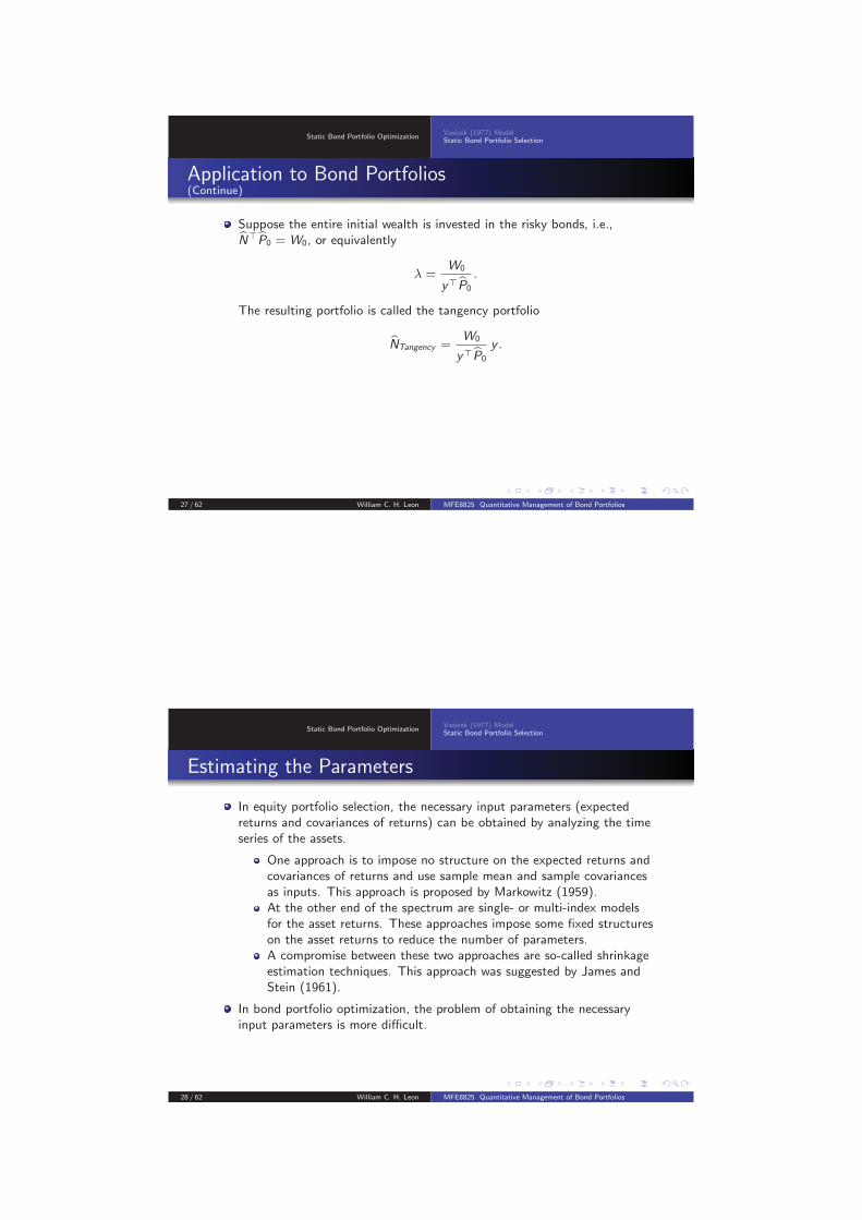
Suppose the entire initial wealth is invested in the risky bonds, i.e.,N̂�P̂0 = W0, or equivalently

λ =W0

y�P̂0

.

The resulting portfolio is called the tangency portfolio

N̂Tangency =W0

y�P̂0

y .



Estimating the Parameters

In equity portfolio selection, the necessary input parameters (expectedreturns and covariances of returns) can be obtained by analyzing the timeseries of the assets.

One approach is to impose no structure on the expected returns andcovariances of returns and use sample mean and sample covariancesas inputs. This approach is proposed by Markowitz (1959).At the other end of the spectrum are single- or multi-index modelsfor the asset returns. These approaches impose some fixed structureson the asset returns to reduce the number of parameters.A compromise between these two approaches are so-called shrinkageestimation techniques. This approach was suggested by James andStein (1961).

In bond portfolio optimization, the problem of obtaining the necessaryinput parameters is more difficult.



Estimating the Parameters(Continue)

For bond portfolio optimization, the expected zero-coupon bond prices atthe investment horizon E (P(T , t)), for T + 1 ≤ t ≤ τ , must be known.

Using simple time series analysis for estimation is not recommended,since bonds have finite maturities and promise to pay the face valueat maturity, so the probability distribution depends on time tomaturity.

Consider a 5-year zero-coupon bond at issuance. The price at the endof the year is random.Consider the same bond 4 years later. Then it has become a 1-yearzero-coupon bond and so the price at the end of the year isnon-random, because it pays the face value at maturity.The return distribution is hence time dependent.

A T -year zero-coupon bond today becomes a (T − 1)-yearzero-coupon bond in one year’s time, hence using the whole timeseries for expected return or variance estimation is not advised, sincethese price observations are not for the same asset.




Estimating E (P(T , t)) (continue).

The problem can be mitigated by analyzing artificial time series forso-called constant maturity bonds.

Since knowledge of the expected zero-bond prices (discount curve) atthe investment horizon is equivalent to the knowledge of theexpected term structure of interest rates, one could also derive theseinput parameters by estimating the term structure of interest ratesfor each day in a certain historical period and estimating the sampledistribution parameters.Any of the classical term structure theories could as well be used toobtain these parameters.Furthermore, dynamic term structure models can be employed.

The expected accrual factors E

(1

P(t,T )

)for every date before the

investment horizon, i.e., 1 ≤ t ≤ T − 1, could be obtained in the sameway using constant maturity bonds.




The covariances between discount factors, Cov (P(T , s),P(T , t)), forT + 1 ≤ s, t ≤ τ , can be obtained by analyzing constant maturity bondsor using dynamic term structure theories.

Classical term structure theories yield no usable information.

The problem becomes more difficult when we consider covariances

between different accrual factors, Cov(

1P(s,T )

, 1P(t,T )

), for

1 ≤ s, t ≤ T − 1, and covariances between accrual factors and discount

factors, Cov(

1P(s,T )

,P(T , t)), for 1 ≤ s ≤ T − 1 and T + 1 ≤ t ≤ τ .

Here the covariance between functions of spot interest rates (i.e.accrual and discount factors) for different dates or with differentmaturity must be derived.




Term structure estimation gives just a snapshot of the current termstructure and no indication of how the term structure moves over time.

So it is impossible to get information about the co-movementsbetween term structures at different dates from the current termstructure.Only dynamic term structure models deliver these kind ofinformation.

The input parameters for the bond portfolio optimization problem (3) canonly be obtained by employing dynamic term structure models and henceimposing a fixed structure on the bond market.

In theory, every dynamic term structure model could be used forobtaining the bond portfolio selection parameters.In practice, there is a trade-off between realism and analyticaltractability.



Estimating the Parameters: Guassian Affine Model

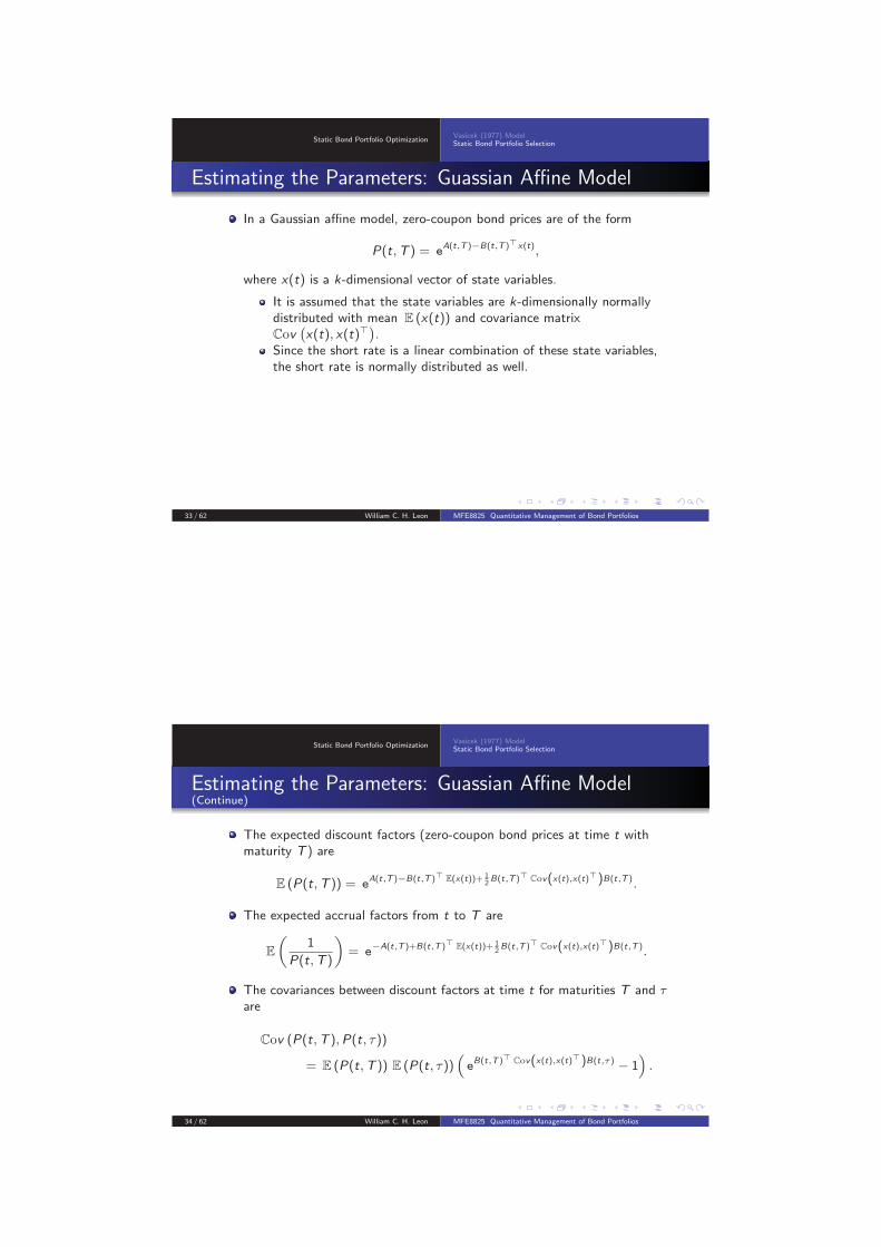
In a Gaussian affine model, zero-coupon bond prices are of the form

P(t,T ) = eA(t,T )−B(t,T )�x(t)

,

where x(t) is a k-dimensional vector of state variables.

It is assumed that the state variables are k-dimensionally normallydistributed with mean E (x(t)) and covariance matrixCov

(x(t), x(t)�

).

Since the short rate is a linear combination of these state variables,the short rate is normally distributed as well.



Estimating the Parameters: Guassian Affine Model(Continue)

The expected discount factors (zero-coupon bond prices at time t withmaturity T ) are

E (P(t,T )) = eA(t,T )−B(t,T )� E(x(t))+ 1

2B(t,T )� Cov(x(t),x(t)�)B(t,T )

.

The expected accrual factors from t to T are

E

(1

P(t,T )

)= e

−A(t,T )+B(t,T )� E(x(t))+ 12B(t,T )� Cov(x(t),x(t)�)B(t,T )

.

The covariances between discount factors at time t for maturities T and τ

are

Cov (P(t,T ),P(t, τ))

= E (P(t,T )) E (P(t, τ))(eB(t,T )� Cov(x(t),x(t)�)B(t,τ) − 1

).



Estimating the Parameters: Guassian Affine Model(Continue)

The covariances between accrual factors for maturities T at time t and τ

are

Cov

(1

P(t,T ),

1

P(τ,T )

)

= E

(1

P(t,T )

)E

(1

P(τ,T )

)(eB(t,T )� Cov(x(t),x(τ)�)B(τ,T ) − 1

).

The covariances between accrual factors at time t with maturity T anddiscount factors at time T with maturity τ are

Cov

(1

P(t,T ),P(T , τ)

)

= E

(1

P(t,T )

)E (P(T , τ))

(e−B(t,T )� Cov(x(t),x(T )�)B(T ,τ) − 1

).



One-Factor Vasicek Model

In the Vasicek (1977) model, the short rate r(t) follows the SDE

dr(t) = κ (θ − r(t)) dt + σ dW (t).

The short rate is the only state variable and it is normally distributed.

The term structure parameters — the current level of the short rate r(0),the mean reversion speed κ, the short rate volatility σ, the mean reversionlevel θ — are normally chosen in such a way to match as closely aspossible the current term structure of interest rates (perhaps subject tosome economically sensible constraints for certain parameters).



One-Factor Vasicek Model(Continue)

The price of a $1-par T -maturity zero-coupon bond is

P(t,T ) = eA(t,T )−B(t,T ) r(t)

,

and the spot rate

R(t,T ) = −A(t,T )

T − t+

B(t,T )

T − tr(t),

where

A(t,T ) =

(θ −

σ2

2κ2

)(B(t,T )− (T − t)

)−

σ2

4κB

2(t,T ),

B(t,T ) =1− e

−κ (T−t)

κ.




The bond portfolio optimization input parameters are as follows:

E (P(t,T )) = eA(t,T )−B(t,T ) E(r(t))+ 1

2B2(t,T )Var(r(t))

,

E

(1

P(t,T )

)= e

−A(t,T )+B(t,T ) E(r(t))+ 12B2(t,T )Var(r(t))

,

Cov (P(t,T ),P(t, τ)) = E (P(t,T )) E (P(t, τ))(eB(t,T )B(t,τ)Var(r(t)) − 1

),

Cov(

1P(t,T )

, 1P(τ,T )

)= E

(1

P(t,T )

)E

(1

P(τ,T )

)(eB(t,T )B(τ,T )Cov(r(t),r(τ)) − 1

),

Cov(

1P(t,T )

,P(T , τ))= E

(1

P(t,T )

)E (P(T , τ))

(e−B(t,T )B(T ,τ)Cov(r(t),r(T )) − 1

).




In addition, the expected value and the variance of the short rate, and thecovariances between short rates at different times are

E( r(T ) | F(t)) = r(t) e−κ(T−t) + θ(1− e

−κ(T−t)),

Var ( r(T ) | F(t)) =σ2

2κ

(1− e

−2κ(T−t))

Cov ( r(T ), r(τ) | F(t)) =σ2

2κ

(1− e

−2κ(T∧τ −t))

(4)




The short rate is the only systematic risk factor in the Vasicek model.

Thus given the distributional properties of the risk factor, we maydeduce the distributional parameters of the assets (the zero-couponbond prices or spot rates).

Using the distribution of the short rate, determine that the distribution ofall spot interest rates at time t are normally distributed with mean

E (R(t,T )) = −A(t,T )

T − t+

B(t,T )

T − tE (r(t))

and variance

Var (R(t,T )) =

(B(t,T )

T − t

)2

Var (r(t)) .




Let τ = 10 and assume the existence of a bond market where zero-couponbonds of maturities 1, 2, . . . , τ trade.

This provides for a large but still manageable set of bonds.

Denote the investment horizon of an investor by T , with 1 ≤ T ≤ τ .

The investor can therefore choose between 9 risky zero-couponbonds and one riskless zero-coupon bond (the T -maturity bond).

Consider two investors who differ in their investment horizon: short-terminvestment horizon (T = 1) and long-term investment horizon (T = 5).

The difference is of importance, since in the short-term case theportfolio value at the investment horizon is solely determined by theterm structure at the investment horizon.In the long-term case, on the other hand, it is also influenced by theterm structures before the investment horizon.



Example(Continue)

Consider a numerical example with the following parameter values:

r(0) κ σ θ

0.0258 0.024 0.1668 0.0153

These parameters describe a normal term structure (i.e.,monotonically increasing spot interest rates) as follow:



Example(Continue)

The current value of the short rate determines the current shape of theterm structure of interest rates, so the shape of the term structure at thesort-term investment horizon is also determined by the future value of theshort rate only.

From (4), the short rate at time t = 1 is normally distributed withmean 0.0255235 and standard deviation 0.0141084.



Example

In addition, the short term rates are more volatile than longer rates.




An important feature of any term structure model is the ability tosimultaneously match the current term structure of interest rates and thecovariance structure of interest rates.

Matching the current term structure would be possible byintroducing a time-dependent drift as in the extended Vasicek model.But matching the covariance structure is impossible as spot interestrates of different maturities are functions of the short rate only, sospot interest rates are perfectly (linearly) correlated.

Empirical observation suggests that spot rates of different maturities arepositively but not perfectly correlated.

The perfect correlation between spot interest rates is one of the mostserious drawbacks of one-factor (affine) interest rate models.



Example: Short-Term Investment Horizon

Zero-coupon bond prices are non-linear functions of spot rates.

The zero-coupon bond price correlation structure is therefore quitesimilar to the spot rate correlation structure.In the Vasicek model, they are perfectly, but non-linearly, correlated.

The correlation matrix of the risky zero-coupon bonds in our numericalexample for the short-term horizon is⎛

⎜⎜⎜⎜⎜⎜⎜⎜⎝

1 0.99 0.99 0.99 0.99 0.99 0.99 0.99 0.99 0.990.99 1 0.99 0.99 0.99 0.99 0.99 0.99 0.99 0.990.99 0.99 1 0.99 0.99 0.99 0.99 0.99 0.99 0.990.99 0.99 0.99 1 0.99 0.99 0.99 0.99 0.99 0.990.99 0.99 0.99 0.99 1 0.99 0.99 0.99 0.99 0.990.99 0.99 0.99 0.99 0.99 1 0.99 0.99 0.99 0.990.99 0.99 0.99 0.99 0.99 0.99 1 0.99 0.99 0.990.99 0.99 0.99 0.99 0.99 0.99 0.99 1 0.99 0.990.99 0.99 0.99 0.99 0.99 0.99 0.99 0.99 1 0.990.99 0.99 0.99 0.99 0.99 0.99 0.99 0.99 0.99 1

⎞⎟⎟⎟⎟⎟⎟⎟⎟⎠

.



Example: Short-Term Investment Horizon(Continue)

Future zero-coupon bond prices are log-normally distributed because theshort rate is normally distributed.

The expected values and standard deviations of zero-coupon bondprices of different maturities at time t = 1 are:

T 1 2 3 4 5 6 7 8 9 10

E (P(1,T )) 1.000 0.974 0.946 0.917 0.888 0.858 0.829 0.801 0.772 0.745√Var (P(1,T )) 0.000 0.013 0.023 0.031 0.037 0.041 0.044 0.047 0.048 0.049

With current prices P(0,T ) we can calculate the (continuouslycompounded) expected returns of the zero-coupon bonds over the nextperiod to be:

T 1 2 3 4 5 6 7 8 9 10

Exp. ret. (%) 2.716 2.975 3.180 3.345 3.477 3.584 3.671 3.743 3.802 3.850




For an initial wealth of W0 = 1, the tangency portfolio is

N̂Tangency =

⎛⎜⎜⎜⎜⎜⎜⎜⎜⎜⎜⎜⎝

19.06−155.91735.31

−2, 198.364, 312.56−5, 543.494, 497.95−2, 088.91

422.8

⎞⎟⎟⎟⎟⎟⎟⎟⎟⎟⎟⎟⎠

.

The portfolio contains enormous long and short positions primarily in the6-, 7- and 8- year zero-coupon bonds.

According to the solution the investor is supposed to buy 4,313 unitsof the 6-year zero-coupon bond for every unit of initial wealth.




The reason for the unrealistic portfolio composition is the following:

An inspection of the tangency portfolio reveals that the sign of theposition alternates, i.e., a long position in the T -year zero-couponbond is followed by a short position in the (T + 1)-year zero-couponbond (and vice versa).Furthermore, for adjacent maturities the correlations are highest.These zero-coupon bonds are therefore considered near perfectsubstitutes (from a diversification perspective) and so (because ofdifferences in expected values and standard deviations) theoptimization procedure tries to exploit a suspected arbitrageopportunity by buying one zero-coupon bond and going short theother.




To obtain portfolios that can be implemented in practice, prohibit shortsales.

A drawback of this measure is the lack of an analytic solution for thebond portfolio optimization problem.Another option would be to restrict the number of zero-bonds theinvestor can buy.




The following table shows the portfolio weights for the ten zero-couponbonds for different expected portfolio values:

E (W1) w1 w2 w3 w4 w5 w6 w7 w8 w9 w10

1.028 1 0 0 0 0 0 0 0 0 0

1.029 0.44 0.56 0 0 0 0 0 0 0 0

1.031 0 0.85 0.15 0 0 0 0 0 0 0

1.032 0 0.18 0.82 0 0 0 0 0 0 0

1.034 0 0 0.45 0.55 0 0 0 0 0 0

1.035 0 0 0 0.58 0.42 0 0 0 0 0

1.037 0 0 0 0 0.59 0.41 0 0 0 0

1.038 0 0 0 0 0 0.41 0.59 0 0 0

1.040 0 0 0 0 0 0 0.37 0.14 0.49 0

1.042 0 0 0 0 0 0 0 0 0 1




These mean-variance efficient portfolios contain at most threezero-coupon bonds.

This is not surprising since all assets are nearly perfectly correlated.Any given expected value can be obtained by a linear combination ofjust two assets since adding more assets would not diversify theportfolio much more.

It is interesting to note, that the portfolios consist of different bonds andnot only positions in the long (maximum maturity) and short (minimummaturity) bond for example.




The following table compares the standard deviations of terminal wealthfor the unconstrained and the short-sale constrained case:

E (W1) Unconstrained Constrained

1.028 0.0000 0.0000

1.029 0.0075 0.0076

1.031 0.0149 0.0151

1.032 0.0224 0.0227

1.034 0.0299 0.0303

1.035 0.0374 0.0379

1.037 0.0449 0.0456

1.038 0.0523 0.0532

1.040 0.0598 0.0609

1.042 0.0673 0.0685

Although the portfolio composition differs significantly, the differencein the portfolio standard deviation for the same expected terminalwealth is small.




The loss in “efficiency” (i.e., higher standard deviation) due to theintroduction of short sale constraints is negligible.

This is not surprising since the assets are nearly perfectly correlatedand are therefore near perfect substitutes.Constraining positions in these assets forces switching but this forcedswitching is relatively costless for the investor, i.e., it raises theportfolio standard deviation only slightly..



Example: Long-Term Investment Horizon

If the investment horizon is greater than one period, then the portfoliovalue at the investment horizon is not only determined by the termstructure at time T but also by the term structures at every date beforeT , because all cash flows that are received before the investment horizonare reinvested at the current spot rate until T .

Changes in the short rate have therefore have radically different effects onshort (maturity less than T ) and long bonds (maturity greater than T ) —analogous to the classical duration analysis (reinvestment risk versusmarket risk).

The major change from the short-term to long-term case therefore isthe correlation matrix of the risky zero-coupon bonds.



Example: Long-Term Investment Horizon(Continue)

The correlation matrix of the risky zero-coupon bonds in our numericalexample for the short-term horizon is⎛⎜⎜⎜⎜⎜⎜⎜⎝

1 0.76 0.67 0.62 −0.59 −0.59 −0.59 −0.59 −0.590.76 1 0.88 0.81 −0.77 −0.77 −0.77 −0.77 −0.770.67 0.88 1 0.93 −0.88 −0.88 −0.88 −0.88 −0.880.62 0.81 0.93 1 −0.95 −0.95 −0.95 −0.95 −0.95−0.59 −0.77 −0.88 −0.95 1 0.99 0.99 0.99 0.99−0.59 −0.77 −0.88 −0.95 0.99 1 0.99 0.99 0.99−0.59 −0.77 −0.88 −0.95 0.99 0.99 1 0.99 0.99−0.59 −0.77 −0.88 −0.95 0.99 0.99 0.99 1 0.99−0.59 −0.77 −0.88 −0.95 0.99 0.99 0.99 0.99 1

⎞⎟⎟⎟⎟⎟⎟⎟⎠

.




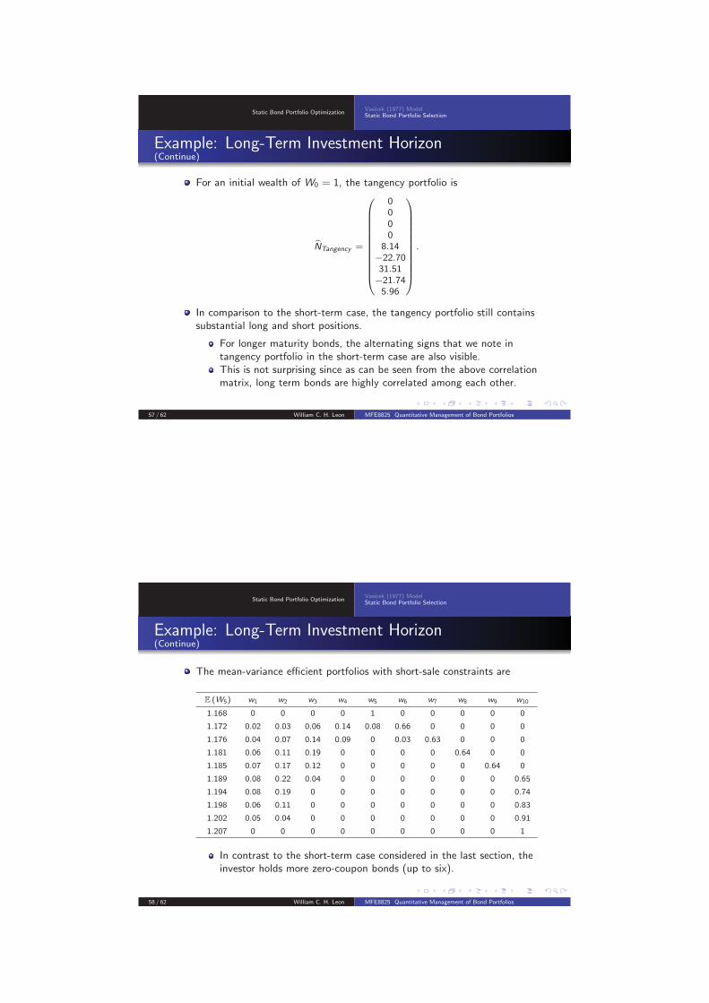
For an initial wealth of W0 = 1, the tangency portfolio is

N̂Tangency =

⎛⎜⎜⎜⎜⎜⎜⎜⎜⎜⎜⎜⎝

0000

8.14−22.7031.51−21.745.96

⎞⎟⎟⎟⎟⎟⎟⎟⎟⎟⎟⎟⎠

.

In comparison to the short-term case, the tangency portfolio still containssubstantial long and short positions.

For longer maturity bonds, the alternating signs that we note intangency portfolio in the short-term case are also visible.This is not surprising since as can be seen from the above correlationmatrix, long term bonds are highly correlated among each other.




The mean-variance efficient portfolios with short-sale constraints are

E (W5) w1 w2 w3 w4 w5 w6 w7 w8 w9 w10

1.168 0 0 0 0 1 0 0 0 0 0

1.172 0.02 0.03 0.06 0.14 0.08 0.66 0 0 0 0

1.176 0.04 0.07 0.14 0.09 0 0.03 0.63 0 0 0

1.181 0.06 0.11 0.19 0 0 0 0 0.64 0 0

1.185 0.07 0.17 0.12 0 0 0 0 0 0.64 0

1.189 0.08 0.22 0.04 0 0 0 0 0 0 0.65

1.194 0.08 0.19 0 0 0 0 0 0 0 0.74

1.198 0.06 0.11 0 0 0 0 0 0 0 0.83

1.202 0.05 0.04 0 0 0 0 0 0 0 0.91

1.207 0 0 0 0 0 0 0 0 0 1

In contrast to the short-term case considered in the last section, theinvestor holds more zero-coupon bonds (up to six).




The structure of the bond portfolios for the long-term and short-termcases differ.

In the short-term case, the maturity of the zero-coupon bonds wasconcentrated at one point on the maturity spectrum.The long-term case produces efficient portfolio that consist of shortand long bonds but no positions in intermediate bonds.




The following table compares the standard deviations of terminal wealthfor the unconstrained and the short-sale constrained case for specificexpected values of terminal wealth:

E (W5) Unconstrained Constrained

1.16775 0.0000 0.0000

1.17208 0.0095 0.0101

1.17641 0.0193 0.0204

1.18075 0.0290 0.0309

1.18508 0.0386 0.0416

1.18941 0.0483 0.0524

1.19374 0.0579 0.0634

1.19808 0.0676 0.0748

1.20241 0.0773 0.0862

1.20674 0.0869 0.0978




The result of the comparison is quite the same as in the short-terminvestment horizon case.

The rise in portfolio standard deviation due to short-sale constraintsis negligible, although the portfolio compositions vary significantly.



Conclusion

The mean-variance approach can be adapted for bond portfolio selection.

For bond market governed by the Vasicek term structure model, anunconstrained optimization yielded portfolios with huge long and shortpositions.

Since these portfolio may not be implemented in the real world, weimposed a short sales constraint.

The resulting constrained optimized portfolios were much more plausible.

Another interesting point is that the introduction of short saleconstraints did not have a significant influence on the portfoliostandard deviations.


mfe8825 quantitative management of bond portfolios

Documents