MAGNETIC METHODKevin Mickus

Department of Geosciences, Southwest Missouri State University, Springfield, MO 65804;mickus@cart1.smsu.edu

OVERVIEW

The magnetic method is a geophysical technique that measures variations in the earth’s magnetic field todetermine the location of subsurface features. This nondestructive technique has numerous applications inengineering and environmental studies, including the location of voids, near-surface faults, igneous dikes, andburied ferromagnetic objects (storage drums, pipes). Magnetic field variations can be interpreted to determinean anomaly’s depth, geometry and magnetic susceptibility.

Magnetic data, measured in gammas and either collected as total field or gradient measurements, mustbe collected in a grid or along a profile with stations spacing between 1 and 10 meters. Relatively little dataprocessing is required for total field measurements as only time varying changes (diurnal variations) are removedfrom the field data. No data processing is required for gradient data.

The interpretation of magnetic data commonly involves the construction of profiles or maps and determiningthe location of obvious magnetic anomalies. If additional interpretation is required, a residual magnetic anomalydue to an object of interest can be determined from the total magnetic field. The interpretation of the residualmagnetic anomalies involves creating models of the subsurface magnetic susceptibility variations to infer ageological cross-section. These models are generally built using a variety of methods ranging from analyticalsolutions to simple geometries to more complex three-dimensional computer algorithms.

INTRODUCTION

The magnetic method of exploring the subsurface is used to either map or locate rock types that containvarying amounts of magnetic susceptible minerals or to locate man-made ferromagnetic (e.g., iron) substances.Thus, the magnetic method has found a broad spectrum of applications in engineering and environmental studiesranging from locating voids and metal containers containing contaminants to mapping dikes that act as barriersto groundwater flow. Table 1 lists the main uses of the magnetic method in shallow geophysical applications.

The magnetic method is relatively easy to perform and inexpensive as it requires little data processing ormanipulation. The technique has good depth penetration compared to other geophysical techniques such asground penetrating radar, high frequency electromagnetics and DC-resistivity. The main disadvantages are thatsubsurface information is obtained only if there are buried ferromagnetic materials and the interpretation ofmagnetic anomalies is nonunique. This nonuniqueness means complementary data (e.g., other geophysicaldata or drill hole data) are required to determine the sources of the magnetic anomalies.

The magnetic method as applied to engineering and environmental studies is relatively straightforward. Asummary of the fundamental aspects including overviews of theory, data collection, processing, andinterpretation is discussed below. For more detailed information on the magnetic technique, numerous paperscovering engineering and environmental aspects are available in the following journals: Geophysics, GeophysicalProspecting, Exploration Geophysics, Journal of Environmental and Engineering Geophysics, and the Journalof Applied Geophysics (formerly Geoexploration). For more detailed investigation on the theoretical backgroundof the magnetic method, the reader is referred to books by Grant and West (1965) and Blakely (1995). Foroverviews of the applied magnetic method, the reader is referred to books by Telford et al. (1990) and Robinsonand Caruh (1988). Recent books by Burger (1992), Vorelsang (1995), Milson (1996), Sharma (1997) andReynolds (1998) contain a chapter on the magnetic method with an emphasis on engineering and environmentalapplications, while the overview paper by Hinze (1990) specifically focuses on engineering and environmentalmagnetic applications.

Table 1. Applications of the Magnetic Method.

Locating

Drums, pipes, cable and metallic objects Buried military ordnance (e.g., shells)

Buried well casings Underground coal burns

Underground voids including mine shafts and adits

Mapping

Archaeological remains (fire pits, cemeteries, garbage pits) Landfills

Concealed dikes and faults Steeply dipping geological contacts

PRINCIPLES OF THE MAGNETIC METHOD

Theory

The theoretical basis of the magnetic method is to a first approximation the same as the gravity method(Mickus, this volume). The main differences between the two techniques are that in the magnetic method, thetotal magnetic field (x, y and z components) is measured, whereas in the gravity method commonly only thez-component is measured. Additionally, the magnetic properties of rocks can vary by several orders ofmagnitude, while the densities of rocks usually only vary by a few percent.

The theory behind the applied magnetic method can be explained by a magnetic dipole in which the basicelements can be seen in a simple bar magnetic (Figure 1). The bar magnetic consists of two poles (dipolar),a positive north-seeking pole and a negative south-seeking pole, and these poles always exist as pairs. Thesetwo poles produce a magnetic field called the magnetic field intensity (H). If a magnetizable body (e.g., iron ormagnetite) is placed in an external magnetic field (e.g., the earth’s magnetic field), it will become magnetizedand produce a secondary magnetic field, determined by the material’s magnetic polarization (M). For lowexternal magnetic fields (e.g., the earth’s), the degree in which the body is magnetized is determined by itsmagnetic susceptibility, k, and is defined as

M = kH. (1)

Magnetic susceptibility is a nondimensional quantity and is the fundamental physical property used inthe magnetic method. The measurement of the total magnetic field, (which includes the external magneticfield and the magnetization) is called the magnetic induction (B) and is written as

B = µo (1 + k)H (2)

where, µo is the magnetic permeability of free space. The units of B are teslas, which is generally too large anumber for applied magnetic work, so gammas (10-9 teslas) are more commonly used. Also, note that B is avector quantity and in most magnetic work today, the amplitude of B is measured and it is called the totalmagnetic field.

Figure 1. Magnetic field due to a simple bar magnetic (adapted from Reynolds, 1998).

Earth’s magnetic field

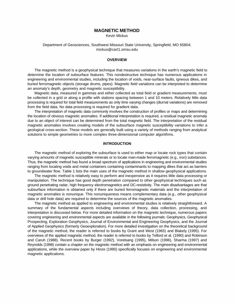
The earth’s magnetic field consists of three components: 1) the main field, 2) the external field and 3)magnetizable materials within the earth’s crust. The main field which accounts for over 99% of the earth’s totalmagnetic field is internal in origin and is thought to be caused by convection currents of conducting material(mainly iron and nickel) within the liquid outer core. The earth’s main magnetic field approximates to a firstdegree a magnetic dipole and is the inducing field for magnetizable objects within the earth’s crust. The mainfield consists of several magnetic elements, which are important in understanding the measured magneticanomaly patterns. These elements include: 1) magnitude of the field (F), 2) magnetic inclination (I) which is thedip of a magnetic compass needle from horizontal (e.g., magnetic south pole is -90o , magnetic north pole is 90o,and magnetic equator is 0o ), and 3) magnetic declination (D) which is the angle between geographic andmagnetic north. Figure 2 shows the relationship between these values. These values are collectively known asthe International Geomagnetic Reference Field (IGRF).

Additionally, the earth’s main magnetic field changes with time due to variations in the motion of theconvection currents within the outer core. These changes (called westward drift or secular variations) cause themagnitude, inclination and declination to change with time. As a consequence, the IGRF is updated every tenyears or so and is revised to give the DGRF (Definitive), which is current reference model of the earth’s magneticfield. The current DGRF can be obtained from the national geophysical data center of the National Oceanic andAtmospheric Agency (NOAA). The use of the DGRF in the magnetic method is explained below in the dataprocessing and interpretation sections.

The external magnetic field (also called diurnal variations) is due to electric currents within the earth’sionosphere. These currents are mainly caused by interactions with plasmas connected with solar winds. Thesediurnal variations fluctuate rapidly but smoothly with time (minutes to hours) with maximum amplitudes varyingfrom 50 to 200 gammas. On some days, these fluctuations are more random with amplitudes of several hundredgammas and are called magnetic storms. These storms are associated with solar flares and sunspot activity,and may persist for hours or several days. During such storms, magnetic surveying should be stopped. Theremoval of diurnal variations from field data is discussed below under data collection and processing.

The magnetizable materials within the earth’s crust create small amplitude magnetic fields that causespatial variations of the earth’s main magnetic field. These materials are the targets of the magnetic method.

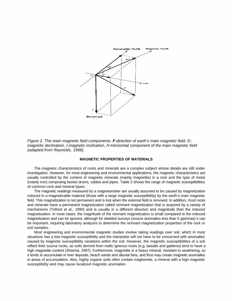
Figure 2. The main magnetic field components. F-direction of earth’s main magnetic field, D-magnetic declination, I-magnetic inclination, H-Horizontal component of the main magnetic field(adapted from Reynolds, 1998).

MAGNETIC PROPERTIES OF MATERIALS

The magnetic characteristics of rocks and minerals are a complex subject whose details are still underinvestigation. However, for most engineering and environmental applications, the magnetic characteristics areusually controlled by the content of magnetic minerals (mainly magnetite) in a rock and the type of metal(mainly iron) composing buried drums, cables and pipes. Table 2 shows the range of magnetic susceptibilitiesof common rock and mineral types.

The magnetic readings measured by a magnetometer are usually assumed to be caused by magnetizationinduced in a magnetizable material (those with a large magnetic susceptibility) by the earth’s main magneticfield. This magnetization is not permanent and is lost when the external field is removed. In addition, most rocksand minerals have a permanent magnetization called remnant magnetization that is acquired by a variety ofmechanisms (Telford et al., 1990) and is usually in a different direction and magnitude than the inducedmagnetization. In most cases, the magnitude of the remnant magnetization is small compared to the inducedmagnetization and can be ignored, although for detailed surveys (source anomalies less than 5 gammas) it canbe important, requiring laboratory analyzes to determine the remnant magnetization properties of the rock orsoil samples.

Most engineering and environmental magnetic studies involve taking readings over soil, which in mostsituations has a low magnetic susceptibility and the interpreter will not have to be concerned with anomaliescaused by magnetic susceptibility variations within the soil. However, the magnetic susceptibilities of a soilreflect their source rocks, as soils derived from mafic igneous rocks (e.g, basalts and gabbros) tend to have ahigh magnetite content (Sharma, 1997). Furthermore, magnetite is a heavy mineral, resistant to weathering, soit tends to accumulate in river deposits, beach sands and alluvial fans, and thus may create magnetic anomaliesin areas of accumulation. Also, highly organic soils often contain maghemite, a mineral with a high magneticsusceptibility and may cause localized magnetic anomalies.

MAGNETIC INSTRUMENTS (MAGNETOMETERS)

The measurement of the earth’s magnetic field using portable magnetometers has greatly improved withinlast 20 years because of the use of integrated circuit devices and the incorporation of internal computers thatallow for the storage, display and simple processing of data as it is being collected. Basically, magnetometersare most commonly used to measure the earth’s total magnetic field and magnetic field gradients. They canbe broken down into two types: 1) proton precession and 2) alkali-vapor. Figure 3 shows a commonly usedproton precession magnetometer.

Proton precession magnetometers are the most commonly used magnetometers and are available in mobileand base station modes. Mobile modes are available with or without internal computers and can have graphicdisplays that store, display and process the data in the field. These instruments consist of a sensor attachedto a nonferrous pole that is either hand carried or attached to the back of the surveyor and a processing unitattached to a shoulder harness positioned in front of the surveyor. The sensor contains a liquid

Table 2. Magnetic susceptibilities of common rocks and minerals

Rock/Mineral Type Susceptibility x 103 (SI units)

DolomiteLimestoneSandstone

ShaleGraniteBasalt

LimoniteHematite

ClayMagnetiteGypsum

Pyrite

0-0.90-3.00-20

0.01-150-50

0.2-1752.5

0.05-350.2

1200-19200-0.110.05-5

Figure 3. Proton precession magnetometer with sensor mounted on an aluminum pole. Photocourtesy of Diane Doser.

(e.g., kerosene, charcoal lighting fluid) that processes a large number of hydrogen ions. If the instrument hasbeen rented, the sensor will be shipped without the flammable liquid, so the surveyor should fill the sensor withthe manufacturers suggested fluid. The processing unit will contain either disposable batteries (usually notshipped with the unit) or more commonly, rechargeable batteries that provide the energy source for themagnetometer.

An advantage of proton precession magnetometers over older magnetometers (e.g., fluxgate) is that thesensor does not have to be oriented. However, these types of magnetometers cannot continuously measure theearth’s magnetic field like fluxgate magnetometers as readings must be taken at least 2-5 seconds apart. Newdevelopments in sensor technology using the Overhauser effect have allowed proton precession magnetometersto take readings every 0.5 seconds. Additionally, proton precession magnetometers will give erroneous readingsin regions with magnetic field gradients of 5000 gammas/m (meter) or larger. These high values are rare but canoccur near surface accumulations of iron. The instruments have accuracies of 0.5 to 1 gammas, total fieldranges from 20,000 to 100,000 gammas and can operate in temperatures from -40o C to 60o C. Base stationmagnetometers can be programmed to record readings down to every 2 seconds. These values provide morethan sufficient accuracy for most engineering and environmental applications throughout the world. Severalmanufacturers sell and rent proton precession magnetometers in North America, including Geometrics, GSMand Scintrex with prices ranging from $6,000 to $8,000 depending on the desired accessories. Additionally,instruments are being developed that contain differential GPS (global positioning systems) units, so bothhorizontal position and magnetic field readings can be obtained simultaneously.

Alkali-vapor magnetometers are basically similar to proton precession magnetometers except for the typeof sensor, which is based on the radiofrequency spectroscopy of an irradiating alkali metal. The two metalscommonly in use are cesium and potassium, with potassium having higher measurement accuracies thancesium. Alkali-vapor magnetometers have a higher sampling rate (10 readings per second) and accuracy (0.01gammas) than proton precession magnetometers. These higher accuracies make them suited for detailedstudies including archaeology, void detection and changes in soil properties. The only drawback is their higherprice ($15,000 to $17,000). These instruments can be obtained from the same manufacturers listed above.

Magnetic gradiometers can be considered as a basic magnetometer system with two different sensors(either proton precession or alkali vapor) spaced 0.2 to 0.3 meters apart (either vertically (more common) orhorizontally). The readings are measured in gammas/m and are useful in determining the lateral boundaries ofburied magnetic features. The advantages of gradiometer measurements are that they are free of noise (e.g.,diurnal variations), suppress regional magnetic anomalies in favor of shallow sources, and the earth’s mainmagnetic field does not have to be removed.

DATA COLLECTION

Magnetic data acquisition can be done on land or by air. Additionally, either total field or magnetic gradientmeasurements can be obtained, as some magnetometers are able to collect both measurementssimultaneously. The data collection techniques are similar for both types of measurements, except that basestations are not required for gradient surveys. Because most engineering and environmental studies cover asmall area and the magnetic sources are usually small in size and magnitude, land-based surveys are mostcommonly performed.

A land-based magnetic survey is a relatively simple task that can be performed by one person. First,stations are surveyed out in either a grid or along profiles perpendicular to suspected linear features (e.g., faults,pipes, dikes). The stations should be located away from any large metallic objects (e.g., fences, pipes,telephone wires, surveyors automobiles). The station spacing depends on the size of the sources and the areato be surveyed with typical spacings ranging from 1 meter when looking for cables to over 10 meters in mappinggeologic contacts. Since elevation variations and changes in latitude and longitude do not influence magneticreadings in most localized surveys, station locations can be determined using a plastic measuring tape (100or 300 meters) (or a measuring wheel) and a compass for orientation. Individual station locations can be markedwith any type of nonferrous marker (e.g., wooden or plastic stake). However, recent developments in

magnetometers have combined a differential GPS with the magnetometer (Geometrics, Inc. and GSM) that candetermine horizontal positions with sub-meter accuracy. Still, most magnetic surveys currently continue to usethe traditional methods outlined above.

Once the stations have been located, the surveyor must tune the magnetometer to the average earth’smagnetic field within the survey area. The correct tuning range can be determined from global magnetic maps(DGRF) usually available with the magnetometer manual, any introductory geophysics book or NOAA. Themagnetometer has an adjustable knob, which can be turned to the earth’s average main field (between 30,000and 65,000 gammas).

The next step in a magnetic survey is to determine if a magnetic base station is required. A base stationmay be needed to remove diurnal variations, which are unpredictable. Unless the source objectives have largemagnetic susceptibilities (e.g., buried drums, pipes) that produce magnetic fields at least one order of amagnitude larger than the diurnal variations, a permanent base station located away from all metallic objectsshould be set up, where the magnetic field is recorded at regular time intervals. This can be done by thesurveyor returning to the base station every one to five minutes or by putting a second automatically recordingmagnetometer at the base station. The former procedure is not recommended for detailed surveys as it maymiss some diurnal changes. Base station magnetometers can be set to record at a given time interval and fordetailed surveys (e.g., archaeology, voids), with the shorter the time period, the better the final results. Resultsfrom small station spacing (1 meter) archaeology studies show that if the base station is recorded at differenttimes as the field magnetometer, small amplitude linear anomalies are produced (Weymouth, 1986).

Once the base station is set up (if needed), the surveyor is ready to take readings. The magnetometersensor usually is connected to an nonferrous pole and is carried by the surveyor. The processing unit isattached to a harness worn by the surveyor (Figure 3). The sensor is commonly set at heights 2 to 2.5 metersabove the ground to avoid small-scale magnetic anomalies due to small iron objects. However, in detailedsurveys these objects may be the target. In such a case, the sensor should be lowered to 0.3 to 0.6 metersabove the ground. Once the survey begins, he/she should not be wearing any ferromagnetic material and at eachstation, at least two readings should be recorded. If the readings are not within 2 gammas, readings should betaken until they do. Also, the time of each reading should be recorded, as they will be used in correcting for thediurnal variations.

DATA PROCESSING

The observed magnetic readings obtained from a magnetic survey reflect the earth’s total magnetic fieldincluding the earth’s main field, diurnal variations and crustal magnetization sources. As compared to the gravitymethod (Mickus, this volume), there are few corrections applied to observed magnetic data. Elevationcorrections are not needed as the vertical gradient of the earth’s magnetic field is less than 0.03 gammas/m.Terrain effects are usually small and neglected unless the topography is caused by steep slopes consisting ofa high magnetic susceptibility material (>0.01 SI) (Sharma, 1997).

The most common processing technique is to remove the diurnal variations using the data collected at abase station. The base station data are plotted versus time (Figure 4). The first reading at the base station is

Figure 4. Typical diurnal variation curve used to remove diurnal variations from total fieldmagnetic data (adapted from Milson, 1996). See text for details.

regarded as the base value and any variations from this value at the base station for later times is subtractedor added to the field data (Figure 4). For example, on Figure 4 the diurnal variation curve at A is approximately25 gammas above the base level so 25 gammas are subtracted from the mobile station recorded at this time.

The only other processing technique that may be applied is to remove the earth’s main magnetic field(DGRF). This is usually performed on surveys covering many kilometers and is not performed for small-scaleengineering and environmental surveys because the earth’s main magnetic changes 0 to 2 gammas/km in east-west and 2-5 gammas/km in north-south directions. Gradiometer data does not require the removal of diurnalvariations or the DGRF.

DATA ANALYSIS AND INTERPRETATION

The object of the magnetic method is to determine information about the earth’s subsurface. The techniquesused to analyze and interpret magnetic data are basically the same as those used in the gravity method. I willhighlight the most commonly used techniques and the reader is referred to the gravity method section (Mickus,this volume) for further details.

Data presentation

Magnetic data are either collected along a profile or in a grid. The most basic interpretation technique is tocollect data along a profile and plot the profile. Then, the profile is examined for obvious magnetic maximum orminimum. Figure 5 shows a profile in central Mexico across a region with known voids (producing magneticminima) embedded in highly magnetic volcanic rocks. If further information on the voids is desired (e.g., depth,size), a residual magnetic anomaly can be determined and subsequently modeled.

Figure 5. Profile of total field magnetic anomalies over suspected and known voids in central Mexico.Boxes represent magnetic minima associated with the voids. (Adapted from Azate et al., 1990).

The most common technique in magnetic interpretation is visualizing a grid ofmagnetic or magnetic gradient data. There are a number of techniques to display gridded data including contourmaps, wire meshes, grey scale or color images. Figure 6 shows magnetic and gradiometer (vertical gradient)data contoured over a buried storage drum. Both surveys indicate magnetic field maxima over the drum withthe magnetic field indicating a north-northeast orientation. The gradient anomaly better defines the orientationplus indicates the ends of tanks. Figure 7 shows a wire mesh representation of magnetic data collected overa buried pipe. The linear, high amplitude anomaly is characteristic of linear features such as pipes and dikes.

Magnetic anomaly patterns

The magnetic field intensities of buried magnetized objects produce different anomaly patterns than gravityanomalies produced by similarly shaped objects. Because of the dipolar nature of magnetic fields, a singlemagnetized body will produce both a positive and negative anomaly and thus is more difficult to interpret thangravity anomalies. The shape of the anomaly depends on the magnetic inclination (I) where the body is located.Figure 8 shows the magnetic anomaly due a positively magnetized sphere at different magnetic inclinations.Note how only at the magnetic north pole (I=90o) is the maximum peak directly over the sphere. At otherinclinations it is offset toward the south until the magnetic equator (I=0o) where the minimum is centered overthe sphere. Thus, the body is not always directly under the maximum or minimum anomaly. Also, note all theanomalies shown in Figure 8 are for north-south profiles. Individual east- west profiles will not show the positiveand negative anomaly patterns and a misinterpretation on the location of the buried body is possible. If possible,north-south profiles should be collected.

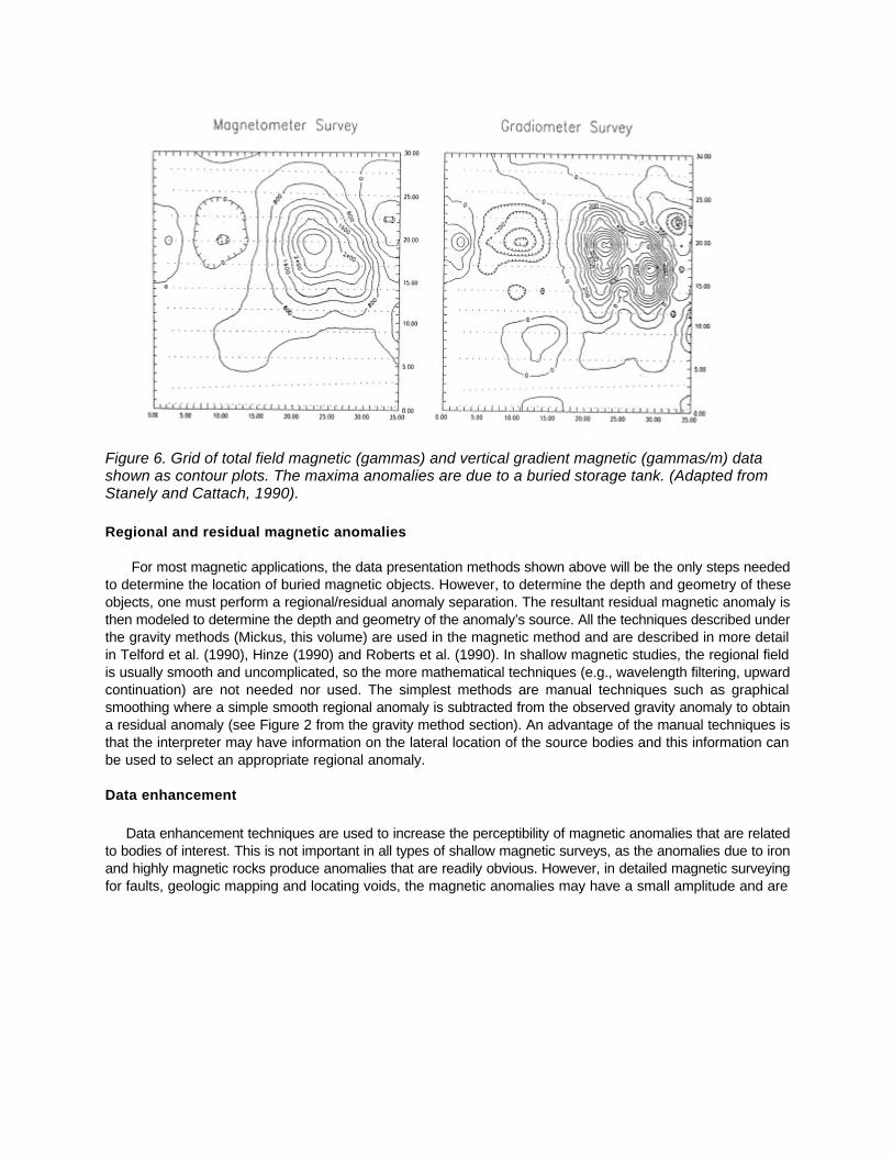
Figure 6. Grid of total field magnetic (gammas) and vertical gradient magnetic (gammas/m) datashown as contour plots. The maxima anomalies are due to a buried storage tank. (Adapted fromStanely and Cattach, 1990).

Regional and residual magnetic anomalies

For most magnetic applications, the data presentation methods shown above will be the only steps neededto determine the location of buried magnetic objects. However, to determine the depth and geometry of theseobjects, one must perform a regional/residual anomaly separation. The resultant residual magnetic anomaly isthen modeled to determine the depth and geometry of the anomaly’s source. All the techniques described underthe gravity methods (Mickus, this volume) are used in the magnetic method and are described in more detailin Telford et al. (1990), Hinze (1990) and Roberts et al. (1990). In shallow magnetic studies, the regional fieldis usually smooth and uncomplicated, so the more mathematical techniques (e.g., wavelength filtering, upwardcontinuation) are not needed nor used. The simplest methods are manual techniques such as graphicalsmoothing where a simple smooth regional anomaly is subtracted from the observed gravity anomaly to obtaina residual anomaly (see Figure 2 from the gravity method section). An advantage of the manual techniques isthat the interpreter may have information on the lateral location of the source bodies and this information canbe used to select an appropriate regional anomaly.

Data enhancement

Data enhancement techniques are used to increase the perceptibility of magnetic anomalies that are relatedto bodies of interest. This is not important in all types of shallow magnetic surveys, as the anomalies due to ironand highly magnetic rocks produce anomalies that are readily obvious. However, in detailed magnetic surveyingfor faults, geologic mapping and locating voids, the magnetic anomalies may have a small amplitude and are

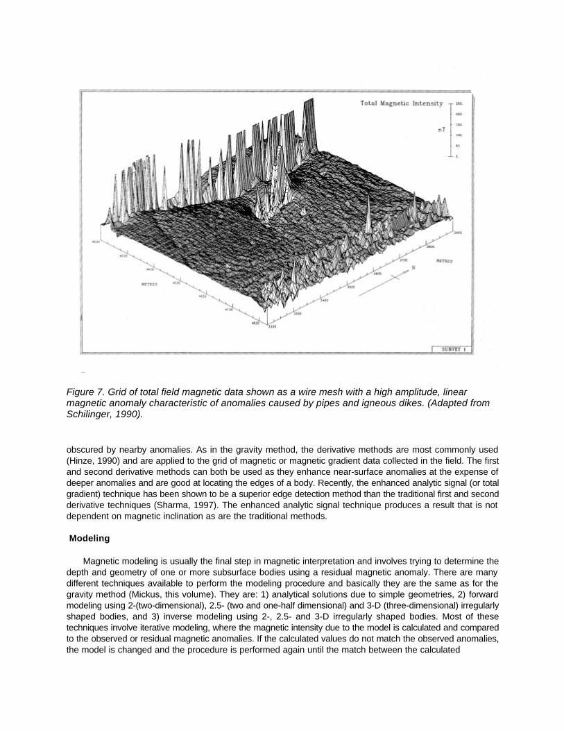
Figure 7. Grid of total field magnetic data shown as a wire mesh with a high amplitude, linearmagnetic anomaly characteristic of anomalies caused by pipes and igneous dikes. (Adapted fromSchilinger, 1990).

obscured by nearby anomalies. As in the gravity method, the derivative methods are most commonly used(Hinze, 1990) and are applied to the grid of magnetic or magnetic gradient data collected in the field. The firstand second derivative methods can both be used as they enhance near-surface anomalies at the expense ofdeeper anomalies and are good at locating the edges of a body. Recently, the enhanced analytic signal (or totalgradient) technique has been shown to be a superior edge detection method than the traditional first and secondderivative techniques (Sharma, 1997). The enhanced analytic signal technique produces a result that is notdependent on magnetic inclination as are the traditional methods.

Modeling

Magnetic modeling is usually the final step in magnetic interpretation and involves trying to determine thedepth and geometry of one or more subsurface bodies using a residual magnetic anomaly. There are manydifferent techniques available to perform the modeling procedure and basically they are the same as for thegravity method (Mickus, this volume). They are: 1) analytical solutions due to simple geometries, 2) forwardmodeling using 2-(two-dimensional), 2.5- (two and one-half dimensional) and 3-D (three-dimensional) irregularlyshaped bodies, and 3) inverse modeling using 2-, 2.5- and 3-D irregularly shaped bodies. Most of thesetechniques involve iterative modeling, where the magnetic intensity due to the model is calculated and comparedto the observed or residual magnetic anomalies. If the calculated values do not match the observed anomalies,the model is changed and the procedure is performed again until the match between the calculated

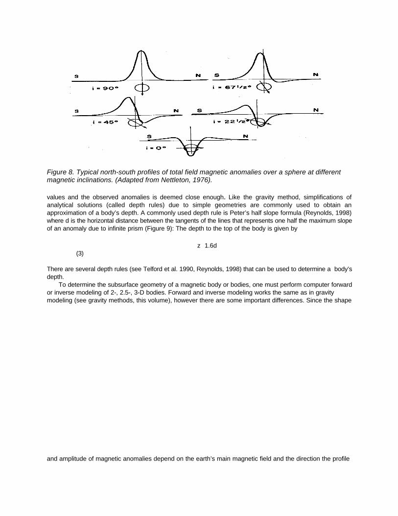
Figure 8. Typical north-south profiles of total field magnetic anomalies over a sphere at differentmagnetic inclinations. (Adapted from Nettleton, 1976).

values and the observed anomalies is deemed close enough. Like the gravity method, simplifications ofanalytical solutions (called depth rules) due to simple geometries are commonly used to obtain anapproximation of a body’s depth. A commonly used depth rule is Peter’s half slope formula (Reynolds, 1998)where d is the horizontal distance between the tangents of the lines that represents one half the maximum slopeof an anomaly due to infinite prism (Figure 9): The depth to the top of the body is given by

z≅1.6d (3)

There are several depth rules (see Telford et al. 1990, Reynolds, 1998) that can be used to determine a body’sdepth.

To determine the subsurface geometry of a magnetic body or bodies, one must perform computer forwardor inverse modeling of 2-, 2.5-, 3-D bodies. Forward and inverse modeling works the same as in gravitymodeling (see gravity methods, this volume), however there are some important differences. Since the shape

and amplitude of magnetic anomalies depend on the earth’s main magnetic field and the direction the profile

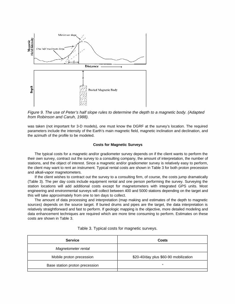
Figure 9. The use of Peter’s half slope rules to determine the depth to a magnetic body. (Adaptedfrom Robinson and Caruh, 1988).

was taken (not important for 3-D models), one must know the DGRF at the survey’s location. The requiredparameters include the intensity of the Earth’s main magnetic field, magnetic inclination and declination, andthe azimuth of the profile to be modeled.

Costs for Magnetic Surveys

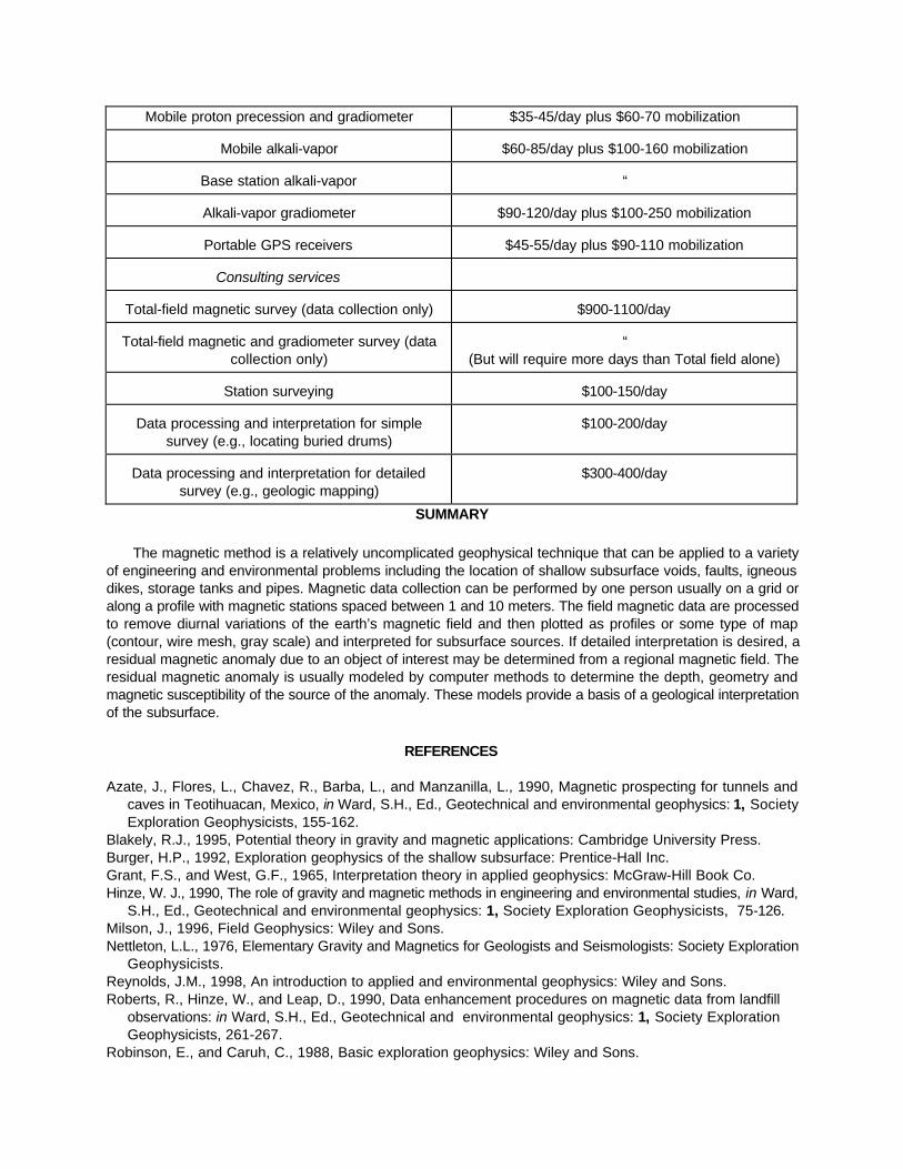
The typical costs for a magnetic and/or gradiometer survey depends on if the client wants to perform thetheir own survey, contract out the survey to a consulting company, the amount of interpretation, the number ofstations, and the object of interest. Since a magnetic and/or gradiometer survey is relatively easy to perform,the client may want to rent an instrument. Typical rental costs are shown in Table 3 for both proton precessionand alkali-vapor magnetometers.

If the client wishes to contract out the survey to a consulting firm, of course, the costs jump dramatically(Table 3). The per day costs include equipment rental and one person performing the survey. Surveying thestation locations will add additional costs except for magnetometers with integrated GPS units. Mostengineering and environmental surveys will collect between 400 and 5000 stations depending on the target andthis will take approximately from one to ten days to collect.

The amount of data processing and interpretation (map making and estimates of the depth to magneticsources) depends on the source target. If buried drums and pipes are the target, the data interpretation isrelatively straightforward and fast to perform. If geologic mapping is the objective, more detailed modeling anddata enhancement techniques are required which are more time consuming to perform. Estimates on thesecosts are shown in Table 3.

Table 3. Typical costs for magnetic surveys.

Service Costs

Magnetometer rental

Mobile proton precession $20-40/day plus $60-90 mobilization

Base station proton precession “

Mobile proton precession and gradiometer $35-45/day plus $60-70 mobilization

Mobile alkali-vapor $60-85/day plus $100-160 mobilization

Base station alkali-vapor “

Alkali-vapor gradiometer $90-120/day plus $100-250 mobilization

Portable GPS receivers $45-55/day plus $90-110 mobilization

Consulting services

Total-field magnetic survey (data collection only) $900-1100/day

Total-field magnetic and gradiometer survey (datacollection only)

“(But will require more days than Total field alone)

Station surveying $100-150/day

Data processing and interpretation for simplesurvey (e.g., locating buried drums)

$100-200/day

Data processing and interpretation for detailedsurvey (e.g., geologic mapping)

$300-400/day

SUMMARY

The magnetic method is a relatively uncomplicated geophysical technique that can be applied to a varietyof engineering and environmental problems including the location of shallow subsurface voids, faults, igneousdikes, storage tanks and pipes. Magnetic data collection can be performed by one person usually on a grid oralong a profile with magnetic stations spaced between 1 and 10 meters. The field magnetic data are processedto remove diurnal variations of the earth’s magnetic field and then plotted as profiles or some type of map(contour, wire mesh, gray scale) and interpreted for subsurface sources. If detailed interpretation is desired, aresidual magnetic anomaly due to an object of interest may be determined from a regional magnetic field. Theresidual magnetic anomaly is usually modeled by computer methods to determine the depth, geometry andmagnetic susceptibility of the source of the anomaly. These models provide a basis of a geological interpretationof the subsurface.

REFERENCES

Azate, J., Flores, L., Chavez, R., Barba, L., and Manzanilla, L., 1990, Magnetic prospecting for tunnels andcaves in Teotihuacan, Mexico, in Ward, S.H., Ed., Geotechnical and environmental geophysics: 1, SocietyExploration Geophysicists, 155-162.

Blakely, R.J., 1995, Potential theory in gravity and magnetic applications: Cambridge University Press.Burger, H.P., 1992, Exploration geophysics of the shallow subsurface: Prentice-Hall Inc.Grant, F.S., and West, G.F., 1965, Interpretation theory in applied geophysics: McGraw-Hill Book Co.Hinze, W. J., 1990, The role of gravity and magnetic methods in engineering and environmental studies, in Ward,

S.H., Ed., Geotechnical and environmental geophysics: 1, Society Exploration Geophysicists, 75-126.Milson, J., 1996, Field Geophysics: Wiley and Sons.Nettleton, L.L., 1976, Elementary Gravity and Magnetics for Geologists and Seismologists: Society Exploration

Geophysicists.Reynolds, J.M., 1998, An introduction to applied and environmental geophysics: Wiley and Sons.Roberts, R., Hinze, W., and Leap, D., 1990, Data enhancement procedures on magnetic data from landfill

observations: in Ward, S.H., Ed., Geotechnical and environmental geophysics: 1, Society ExplorationGeophysicists, 261-267.

Robinson, E., and Caruh, C., 1988, Basic exploration geophysics: Wiley and Sons.

Schilinger, C.M., 1990, Magnetometer and gradiometer surveys for detection of underground storage tanks:Bulletin Association Engineering Geologists, 27, 37-50.

Sharma, P.V., 1997, Environmental and engineering geophysics: Cambridge Univ. Press.Stanely, J., and Cattach, M., 1990, The use of high-definition magnetics in engineering site investigation:

Exploration Geophysics, 21, 91-103.Telford, W.M., Geldart, L.P., and Sheriff, R.E., 1990, Applied Geophysics, Cambridge Univ. Press.Vogelsang, D., 1995, Environmental Geophysics: Springer-Verlag.Weymouth, J.W., 1986, Archaeological site surveying program at the University of Nebraska: Geophysics,

51, 538-552.