microbenchmarks in java and c#sestoft/papers/benchmarking.pdf · 2015-09-16 · microbenchmarks in...

Microbenchmarks in Java and C#

Peter Sestoft ([email protected])

IT University of Copenhagen, Denmark

Version 0.8.0 of 2015-09-16

Abstract: Sometimes one wants to measure the speed of software, for instance, to measure whether a

new way to solve a problem is faster than the old one. Making such time measurements and microbench-

marks requires considerable care, especially on managed platforms like the Java Virtual Machine and

Microsoft’s Common Language Infrastructure (.NET), or else the results may be arbitrary and mislead-

ing.

Here we give some advice on running microbenchmarks, in particular for managed platforms. Most

examples are in Java but the advice applies to any language executed on a managed platform, including

Scala, C# and F#. This version uses Java functional interfaces and requires Java 8.

1 The challenge of managed platforms

Measuring the execution time of a piece of software is an experimental activity, involving the software

and a computer system, itself consisting of much (systems) software and some hardware. Whereas bi-

ological experiments, such as measuring bacterial growth, are influenced by natural variation and many

unknown circumstances, software performance measurements may seem straightforward: in principle,

everything is man-made and under the experimenter’s control. However, in practice, software perfor-

mance measurements are influenced by so many factors, and modern computer systems are growing so

complex, that software experiments increasingly resemble biological experiments.

One source of complications is the widespread use of managed execution platforms, such as the Java

Virtual Machine (JVM), Microsoft’s Common Language Infrastructure (.NET), and high-performance

Javascript implementations such as Google’s v8 engine. These managed execution platforms typically

accept software in intermediate form (bytecode or even source code) and compile that intermediate

form to real machine code at runtime, by so-called just-in-time compilation. This seriously affects the

execution time, for several reasons.

First, the just-in-time compilation process itself takes some time, contributing start-up overhead.

Second, just-in-time compilation typically involves adaptive optimizations, based on the execution counts

actually observed at runtime. If the code is executed only a few times, the just-in-time compiler may

quickly generate slow code; if it is executed many times, the just-in-time compiler may spend more time

generating faster code. Hence the speed of a piece of code is likely to depend on input parameters in

complex ways, making it dubious to extrapolate from measurements with short execution times. Third,

the just-in-time compiler, or its designers, will try to avoid time-consuming code analyses. This means

that code that gets optimized well in a simple context may not be optimized at all in a more complex

context that is harder to analyse. Fourth, managed platforms typically have automatic memory manage-

ment, which in practice means that the garbage collector may decide to run at any time, affecting the

code execution measurements in unpredictable ways.

In addition, all this software typically runs on top of complex operating systems (MacOS, Linux,

Windows 7), complex processors (Intel i5, AMD), and complex memory management systems (caches,

memory management hardware), adding further uncontrollable parameters.

1

2 Measuring execution time

The time spent executing some software may be measured in many different ways: wall-clock time or

elapsed time (that is, the total amount of real time that has passed), CPU time spent by the client code

only (measured by the operating system), CPU time spent by the client code and any system calls it

made, CPU time plus time spent doing input and output, and more.

Here we shall measure simply wall-clock time, because this simplifies comparison between plat-

forms (Java, C#, Linux, MacOS, Windows). Measuring wall-clock time, not just CPU time (or even

CPU cycles), means that the measurements are easily affected by other processes running on the same

machine, so one should terminate as many of those processes as possible. See warnings in section 7.

2.1 A simple timer class for Java

This Java class Timer measures wall-clock time and is portable over most Java execution platforms (in

particular Linux, MacOS and Windows):

public class Timer {

private long start, spent = 0;

public Timer() { play(); }

public double check() { return (System.nanoTime()-start+spent)/1e9; }

public void pause() { spent += System.nanoTime()-start; }

public void play() { start = System.nanoTime(); }

}

The timer is started when the Timer object is created. The elapsed time (in seconds) is returned whenever

check() is called. The methods pause and play may be used to suspend and resume the timer; see

section 5.

2.2 A simple timer class for C#

A similar Timer class for C# can be defined like this:

public class Timer {

private readonly System.Diagnostics.Stopwatch stopwatch

= new System.Diagnostics.Stopwatch();

public Timer() { Play(); }

public double Check() { return stopwatch.ElapsedMilliseconds/1000.0; }

public void Pause() { stopwatch.Stop(); }

public void Play() { stopwatch.Start(); }

}

Like the Java Timer class it measures wall-clock time in seconds.

3 Developing basic microbenchmark code

Our microbenchmark code is intended to measure CPU time, memory access time and any associated

systems overhead. This may be used to compare different data structures or algorithms, to compare

different implementations of methods, or to compare speed of access to different levels of the memory

hierarchy.

The microbenchmark code here is not suitable for measuring end-to-end performance of systems

that involve disk accesses or network accesses, in particular when these involve asynchronous operations

such as non-blocking input-output operations.

Let us assume that you want to measure the time to call and execute this little method:

2

private static double multiply(int i) {

double x = 1.1 * (double)(i & 0xFF);

return x * x * x * x * x * x * x * x * x * x

* x * x * x * x * x * x * x * x * x * x;

}

Each call to the method performs 20 floating-point multiplications, as well as an integer bitwise “and”

(&) and a conversion of a 32-bit int to a 64-bit double. Performing these operations should take

20–50 CPU cycles, or 8–20 nanoseconds (ns), on a contemporary laptop or desktop Intel i7 CPU with a

clock frequency of 2.4 GHz, since 20 / 2.4 GHz equals 8.3 ns.

The purpose of the (double)(i & 0xFF) part is to make the computation dependent on the

unknown argument i instead of a constant. The (i & 0xFF) part just makes sure that x is between

0 and 255, in other words, it does not grow very large. The dependency on the argument i prevents

the compiler from simply performing the multiplications once and for all (before the method is called),

either when the program is compiled to bytecode by javac, or when the bytecode is compiled to native

machine code by the java just-in-time compiler.

We shall now consider a sequence of increasingly meaningful ways to measure the time it takes to

perform a call of method multiply.

3.1 Mark0: measure one operation (useless)

The simplest attempt is to start the timer, call the function, and measure and print the elapsed time in

nanoseconds (ns):

public static void Mark0() { // USELESS

Timer t = new Timer();

double dummy = multiply(10);

double time = t.check() * 1e9;

System.out.printf("%6.1f ns%n", time);

}

However, this is useless for many reasons. Running a Java program that calls Mark0 from the command

line a couple of times may produce output like this:

5249.0 ns

4992.0 ns

5098.0 ns

First, this is far too slow for 20 multiplications, and secondly, the numbers may vary widely. Possibly

we are measuring the time it takes to compile the multiply method (and maybe the Timer’s check

method) from bytecode to native x86 code; it is hard to know, but the results are certainly wrong.

Moreover, on some platforms the timer resolution is so low that the result is always 0.0 ns, which is

equally wrong. From this measurement you can conclude nothing at all.

3.2 Mark1: measure many operations

A much better approach is to start the timer, execute the function many times, here 1 million times, and

print the elapsed time divided by 1 million:

public static void Mark1() { // NEARLY USELESS


Integer count = 1_000_000;

for (int i=0; i<count; i++) {

3

double dummy = multiply(i);

}

double time = t.check() * 1e9 / count;


}

The CPU now also has to perform the test on loop counter i, the increment i++ and so on, which affects

the time spent. On a modern CPU such as Intel Core 2 or i5 or i7, instruction-level parallelism means

that these operations are likely to be executed in parallel with the multiplication. In fact, the results of a

couple of runs seem somewhat reasonable:

5.0 ns

5.5 ns

5.0 ns

However, the variation from run to run still appears unpleasantly high, and the times themselves implau-

sibly low. Worse, if you increase count to 100 million in an attempt to reduce variation between runs,

then the execution time drops to 0.0 ns or 0.1 ns, highly implausible:

0.1 ns

0.1 ns

0.0 ns

3.3 Mark2: avoid dead code elimination

What happened in Mark1 probably was that the JIT compiler realized that the result of multiply was

never used, and so the loop has no effect at all — it is dead code — and therefore the loop was removed

completely. Hence the implausibly low execution times.

To avoid this, we change the benchmark loop to pretend that the result is used, by adding it to a

dummy variable whose value is returned by the method:

public static double Mark2() {


int count = 100_000_000;

double dummy = 0.0;

for (int i=0; i<count; i++)

dummy += multiply(i);



return dummy;

}

Running this program multiple times we now get more consistent and plausible results, like these:

30.5 ns

30.4 ns

30.3 ns

These execution times are somewhat reasonable for a method call, 20 floating-point multiplications, one

floating-point addition, and a few integer operations, although somewhat slow compared to our 8–20

ns estimate made above. And in fact, with another virtual machine or slightly different hardware, one

might get reproducible execution times such as 16.6 ns.

4

3.4 Mark3: automate multiple runs

Our next step is a simple convenience to automate the execution of multiple runs, instead of having to

run the entire program multiple times:


int n = 10;

int count = 100_000_000;

double dummy = 0.0;

for (int j=0; j<n; j++) {






}

return dummy;

}

The output gives a good idea of the variation, which in this particular case is very small:

30.7 ns

30.3 ns

30.1 ns

30.7 ns

30.5 ns

30.4 ns

30.9 ns

30.3 ns

30.5 ns

30.8 ns

This is much more satisfactory. All the iterations take nearly the same amount of time, and the results

are consistent with the Mark2 measurements.

3.5 Mark4: compute standard deviation

Instead of printing all the measurements we could compute and print the empirical mean and standard

deviation of the measurements:


int n = 10;

int count = 100_000_000;

double dummy = 0.0;

double st = 0.0, sst = 0.0;






st += time;

sst += time * time;

}

double mean = st/n, sdev = Math.sqrt((sst - mean*mean*n)/(n-1));

System.out.printf("%6.1f ns +/- %6.3f %n", mean, sdev);

return dummy;

}

5

This executes the same benchmark runs but reduces the amount of output:

30.3 ns +/- 0.137

This result is pleasantly consistent with those obtained from Mark3 above.

In general, one should not expect such consistency for very short methods. For instance, if one

simplifies multiply to just return the x computed in the first line, then it is possible that all iterations

of Mark3 reports 1.7 ns/call, yet Mark4 would find that the mean is 2.2 ns. The exact cause for this

observation is unknown, but probably it just indicates that one cannot reliably measure the execution

time of very small methods.

The standard deviation is a kind of summary of the variation between the 10 measurements, remov-

ing the need to inspect them all manually. More precisely, the central limit theorem from statistics tells

us that the average of n independent identically distributed observations t1, . . . , tn tends to follow the

normal distribution N(µ, σ2), also known as the Gaussian distribution, when n tends to infinity, where

µ and σ may be estimated like this:

µ = 1

n

∑nj=1

tj

σ =√

1

n−1

∑nj=1

(tj − µ)2

Moreover, from the distribution function of the normal distribution N(µ, σ2) we know that 68.3% of

the observations should fall within the interval [µ− σ, µ+ σ] and 95.4% of the observations should fall

within the wider interval [µ− 2σ, µ + 2σ], see figure 1.

Figure 1: The density function of the normal distribution N(0, 1). The area under the curve between the

blue lines at −1 and +1 is 68.3% of the total area under the curve. Hence 68.3% of the observations

should fall between −1 and +1, that is, at most one standard deviation from the mean. Similarly, 95.4%

of the observations fall between −2 and +2, that is, at most two standard deviations from the mean.

Applying this theory to the Mark4measurement above, we conclude that there is 68.3% chance that

the actual execution time for multiply is between 30.163 ns and 30.437 ns, and 95.4% chance that it

is between 30.026 and 30.574 ns. Now this theory is based on the number n of observations being very

large, as n tends to infinity, but our n is a modest 10, namely the number of repeated measurements.

For a more trustworthy application of the theory, you may choose a larger value of n, but then your

benchmarks take that much longer to run.

6

3.6 Mark5: choosing the iteration count automatically

The number of iterations (count equals 100 million) used above was rather arbitrarily chosen. While it

probably is sensible for the small multiply function, it may be far too large when measuring a more

time-consuming function. To “automate” the choice of count, and to see how the mean and standard

deviation are affected by the number of iterations, we add an outer loop. In this outer loop we double

the count until the execution time is at least 0.25 seconds:


int n = 10, count = 1, totalCount = 0;

double dummy = 0.0, runningTime = 0.0;

do {

count *= 2;

double st = 0.0, sst = 0.0;





runningTime = t.check();

double time = runningTime * 1e9 / count;

st += time;

sst += time * time;

totalCount += count;

}


System.out.printf("%6.1f ns +/- %8.2f %10d%n", mean, sdev, count);

} while (runningTime < 0.25 && count < Integer.MAX_VALUE/2);

return dummy / totalCount;

}

This might produce output like this:

100.0 ns +/- 200.00 2

100.0 ns +/- 122.47 4

62.5 ns +/- 62.50 8

50.0 ns +/- 37.50 16

46.9 ns +/- 15.63 32

40.6 ns +/- 10.36 64

39.8 ns +/- 2.34 128

36.3 ns +/- 1.79 256

36.5 ns +/- 1.25 512

35.6 ns +/- 0.49 1024

111.1 ns +/- 232.18 2048

36.1 ns +/- 1.75 4096

33.7 ns +/- 0.84 8192

32.5 ns +/- 1.07 16384

35.6 ns +/- 4.84 32768

30.4 ns +/- 0.26 65536

33.1 ns +/- 5.06 131072

30.3 ns +/- 0.49 262144

30.0 ns +/- 0.20 524288

30.6 ns +/- 1.34 1048576

30.2 ns +/- 0.24 2097152

30.5 ns +/- 0.35 4194304

30.3 ns +/- 0.20 8388608

7

As one might hope, the mean (first column) converges towards 30.3 ns, and the standard deviation

(second column) becomes smaller, as count (third column) grows. The end result is also consistent

with that of Mark4. The exception is the sudden increase to 111.1 ns for iteration count 2048, but we

also see that the standard deviation is very large in that case, which tells us we can have no confidence

in that result. This outlier measurement may be caused by the garbage collector accidentally performing

some work at that time, or the just-in-time compiler, or some other external disturbance.

A side remark: The second half of the do-while loop condition prevents count from overflowing

the int range. This effectively limits the iteration count to 1 billion (109), but that is sufficient for

methods with execution time 2.5 ns or more, and it would be meaningless to benchmark functions

that are faster than that. Alternatively, to avoid overflow one might declare count as a 64-bit long,

but on some architectures the overhead of long arithmetics and comparisons might distort the actual

measurement results.

3.7 Summary of benchmarking functions

Let us summarize the steps that led to the design of our benchmarking function Mark5:

• Mark0 measured a single function call, but that included some unknown virtual machine start up

costs, and also ran for too short a time to be measured accurately, and hence was useless.

• Mark1 improved on Mark0 by measuring a large number of function calls, hence distribution

the start up costs on these. Unfortunately, the just-in-time compiler might optimize away all the

function calls because their results were not used.

• Mark2 improved on Mark1 by accumulating the function results in the dummy variable and

returning its value, thereby preventing the just-in-time compiler from optimizing away the calls.

Unfortunately, it made just one timing measurement (of count function calls), thus not allowing

us to estimate the reliability of the reported average.

• Mark3 improved on Mark2 by making a set of ten measurements, so one can inspect the variation

in the averages. Unfortunately, visual inspection of the variation is cumbersome when making

many sets of measurements, for instance of many different functions.

• Mark4 improved on Mark3 by additionally computing the standard deviation and printing only

the average and the standard deviation for each set of 10 measurements. Unfortunately, the number

count of function calls in each set of measurements was fixed but chosen arbitrarily, and might

be far too large for some functions we want to benchmark.

• Mark5 improved on Mark4 by choosing count to be 2 initially, and doubling it until the running

time of the last measurement (in a set) was at least a quarter second, long enough to avoid problems

with virtual machine startup and clock resolution.

Hence we have arrived at a somewhat reliable and usable benchmarking function, Mark5.

8

4 General microbenchmark code

Now that we are happy with the basic benchmarking code, we generalize it so that we can measure many

different functions (not just multiply) more easily, for instance to compare alternative algorithms or

implementations.

4.1 Mark6: generalize to any function

The functional interface java.util.function.IntToDoubleFunction in Java 8 has method applyAsDouble:

public interface IntToDoubleFunction {

double applyAsDouble(int i);

}

Any function from int to double can be represented by this interface. A general benchmarking

function Mark6 would simply take an IntToDoubleFunction as argument and hence work for any such

function, not just multiply:

public static double Mark6(String msg, IntToDoubleFunction f) {

int n = 10, count = 1, totalCount = 0;

double dummy = 0.0, runningTime = 0.0, st = 0.0, sst = 0.0;

do {

count *= 2;

st = sst = 0.0;




dummy += f.applyAsDouble(i);



st += time;

sst += time * time;


}


System.out.printf("%-25s %15.1f %10.2f %10d%n", msg, mean, sdev, count);



}

In addition to the method to be benchmarked, the benchmarking function takes as argument a string

msg that describes that function. Also, the printed output has been simplified so that it is easier to

further process with other software, for instance to make charts with gnuplot (section 9) or MS Excel

(section 10).

We can now apply the general benchmarking method Mark6 to Benchmark::multiply, which

is a method reference denoting the multiply method:

Mark6("multiply", Benchmark::multiply);

The result may look like this, which says that function multiply used on average 30.3 ns per call

when called 8 million times, and that the standard deviation between 10 such runs was 0.20:

9

multiply 750.0 1289.38 2

multiply 200.0 100.00 4

multiply 212.5 80.04 8

multiply 206.3 40.02 16

multiply 209.4 93.80 32

multiply 100.0 62.58 64

multiply 48.4 5.85 128

multiply 48.0 1.79 256

multiply 48.2 6.18 512

multiply 42.6 0.65 1024

multiply 42.3 1.69 2048

multiply 41.7 2.43 4096

multiply 34.0 1.73 8192

multiply 33.2 0.57 16384

multiply 31.2 1.74 32768

multiply 35.8 6.24 65536

multiply 30.8 0.90 131072

multiply 30.9 0.60 262144

multiply 30.8 0.69 524288

multiply 31.2 1.20 1048576

multiply 30.2 0.15 2097152

multiply 30.3 0.24 4194304

multiply 30.3 0.20 8388608

This is neat, and consistent with all the previous measurements. In any case, it seems that the extra

call through the functional interface IntToDoubleFunction does not in itself slow down the program,

presumably because the just-in-time (JIT) compiler optimizes it away.

4.2 Mark7: print only the final measurement

When the mean converges and the standard deviation decreases, as in the multiply example just

shown, it would suffice to print the results for the final value of count, which can be achieved simply

by moving the computation and printing of mean and sdev out of the do-while loop in Mark6. This

is the only difference between Mark6 and the new Mark7:


...

do {

...



System.out.printf("%-25s %15.1f %10.2f %10d%n", msg, mean, sdev, count);


}

Printing just the final value makes sense if one assumes that the optimizations performed by the just-in-

time compiler and runtime system stabilize eventually, but not if the just-in-time compiler indefinitely

tries and retries new optimizations and generates new machine code.

Using Mark7 on multiply is easy:

Mark7("multiply", Benchmark::multiply);

and produce a result consistent with the final result of Mark6:

multiply 30.1 0.16 8388608

10

When benchmarking many different functions, the Mark7 simplification of the output considerably im-

proves the overview, and we can now benchmark many functions in one go. Here we pass a lambda

expression (of type IntToDoubleFunction) in each call:

Mark7("pow", i -> Math.pow(10.0, 0.1 * (i & 0xFF)));

Mark7("exp", i -> Math.exp(0.1 * (i & 0xFF)));

Mark7("log", i -> Math.log(0.1 + 0.1 * (i & 0xFF)));

Mark7("sin", i -> Math.sin(0.1 * (i & 0xFF)));

Mark7("cos", i -> Math.cos(0.1 * (i & 0xFF)));

Mark7("tan", i -> Math.tan(0.1 * (i & 0xFF)));

Mark7("asin", i -> Math.asin(1.0/256.0 * (i & 0xFF)));

Mark7("acos", i -> Math.acos(1.0/256.0 * (i & 0xFF)));

Mark7("atan", i -> Math.atan(1.0/256.0 * (i & 0xFF)));

This may produce results such as the following:

pow 76.0 0.57 4194304

exp 55.0 0.41 8388608

log 31.9 0.55 8388608

sin 116.1 0.61 4194304

cos 116.1 0.49 4194304

tan 143.4 1.40 2097152

asin 232.1 2.70 2097152

acos 216.4 2.30 2097152

atan 54.1 0.27 8388608

A word of warning: Whereas these results are quite reliable for more complicated functions such as

pow, exp and trigonometry, the result for method multiply or even simpler ones may not be. What

is measured in that case is really the just-in-time compiler’s ability to inline function calls and schedule

instructions in a particular context. For instance, on other hardware and with a different Java imple-

mentation, we have found the execution time for multiply to be 18.4 ns, 13.8 ns, and 16.5 ns, all

apparently with low standard deviation. Those results were heavily influenced, in mysterious ways, by

other code executed before and after (!) the code being benchmarked.

4.3 Mark8: problem size parameters

Often, the execution time of a method depends on the problem size. For instance, we may want to

measure the execution time of a binary array search method:

static int binarySearch(int x, int[] arr) { ... }

The method returns the index of item x in sorted array arr, or returns −1 if x is not in the array.

Clearly the execution time depends on the size of the array, so we would want to measure it for a range

of such array sizes. Moreover, we would like the array size to be printed along with the measured mean

execution time and the standard deviation.

As a further generalization, we want to make the rather arbitrarily chosen repeat count (10) and

minimal execution time (0.25 s) into user-controllable parameters.

Thus we define yet another benchmarking method that simply takes several additional parameters:

public static double Mark8(String msg, String info, IntToDoubleFunction f,

int n, double minTime) {

int count = 1, totalCount = 0;


11

do {

count *= 2;

st = sst = 0.0;







st += time;

sst += time * time;


}

} while (runningTime < minTime && count < Integer.MAX_VALUE/2);


System.out.printf("%-25s %s%15.1f %10.2f %10d%n", msg, info, mean, sdev, count);


}

A couple of convenient overloads with useful parameter values include these, where the first one is

equivalent to the old Mark7:


return Mark8(msg, "", f, 10, 0.25);

}

public static double Mark8(String msg, String info, IntToDoubleFunction f) {

return Mark8(msg, info, f, 10, 0.25);

}

To measure the binary search execution time for a range of array sizes, we run this benchmark:

for (int size = 100; size <= 10_000_000; size *= 2) {

final int[] intArray = SearchAndSort.fillIntArray(size); // sorted [0,1,...]

final int successItem = (int)(0.49 * size);

Mark8("binary_search_success",

String.format("%8d", size),

i -> SearchAndSort.binarySearch(successItem, intArray));

}

Notice the use of String.format to make sure that the info string always has the same length,

so that the ASCII output continues to line up in columns. Indeed, a possible result from running this

benchmark may be:

binary_search_success 100 4.4 0.05 67108864












12






This looks neat, but it turns out that these results probably seriously underestimate realistic execution

times, not because we measure in the wrong way, but because we measure the wrong thing: it is not

realistic to search for the same item again and again. See section 11.1 for a discussion and more realistic

results.

4.4 Collecting and further processing benchmark results

The output of a benchmark run, as shown for instance at the end of section 4.3, can be piped into a file

for further processing by other software (see also section 9):

$ java Benchmark > binary-search.out

5 Benchmarks that require setup

Sometimes a method that we want to benchmark will modify or destroy the data it works on, so the data

must be restored before each execution of the code. For instance, an array sort procedure will leave the

argument array sorted, and since there is little point in measuring how long it takes to sort an already-

sorted array, the array disorder must be reestablished before the next benchmark run, for instance by

randomly shuffling the array.

A general method for this purpose can be defined by declaring an abstract class Benchmarkable that

implements the functional interface IntToDoubleFunction and in addition has a setup method that sets

up data before performing the measurement:

public abstract class Benchmarkable implements IntToDoubleFunction {

public void setup() { }

public abstract double applyAsDouble(int i);

}

We define new variant of method Mark8 that takes a Benchmarkable argument, and avoids measuring

the setup time by suspending the timer (section 2.1) before the call to setup and resuming the timer

after it:

public static double Mark8Setup(String msg, String info, Benchmarkable f,

int n, double minTime) {

int count = 1, totalCount = 0;


do {

count *= 2;

st = sst = 0.0;



for (int i=0; i<count; i++) {

t.pause();

f.setup();

t.play();


}

13



st += time;

sst += time * time;


}

} while (runningTime < minTime && count < Integer.MAX_VALUE/2);


System.out.printf("%-25s %s%15.1f %10.2f %10d%n", msg, info, mean, sdev, count);

return dummy;

}

This method should be used only to benchmark functions that take some substantial amount of time (say,

at least 100 ns/call) to execute, otherwise the benchmark will mostly measure the amount of time it takes

to suspend and resume the timer.

To compare three algorithms for array sort: selection sort, quicksort, and heap sort, we may use a

random permutation (shuffle) of an array of 10,000 integers, like this:

final int[] intArray = SearchAndSort.fillIntArray(10_000);

Mark8Setup("selection_sort",

new Benchmarkable() {

public void setup() { SearchAndSort.shuffle(intArray); }

public double applyAsDouble(int i)

{ SearchAndSort.selsort(intArray); return 0.0; } });

Mark8Setup("quicksort",




{ SearchAndSort.quicksort(intArray); return 0.0; } });

Mark8Setup("heapsort",




{ SearchAndSort.heapsort(intArray); return 0.0; } });

Here are the results from one execution. They show that selection sort is more than 120 times slower

than quicksort, and that heap sort is 1.18 times slower than quicksort, on arrays with 10000 elements:

selection_sort 38147737.5 221026.39 8

quicksort 767679.5 2299.36 512

heapsort 829134.2 8257.46 512

6 Execution time as a function of problem size

We can further use Mark8Setup to measure the time to sort arrays of size 100, 200, 400, and so on:


final int[] intArray = SearchAndSort.fillIntArray(size);

Mark8Setup("quicksort",





{ SearchAndSort.quicksort(intArray); return 0.0; } });

14

}

System.out.printf("%n%n"); // data set divider

... and similarly for other sorting algorithms ...

The result may look like this:

quicksort 100 4486.7 60.39 65536

quicksort 200 9882.7 23.95 32768

quicksort 400 21778.9 81.49 16384

quicksort 800 47738.3 246.73 8192

quicksort 1600 102736.4 328.70 4096

quicksort 3200 222186.8 1601.44 2048

quicksort 6400 480137.4 7955.89 1024

quicksort 12800 1005463.7 1390.13 256

quicksort 25600 2147215.6 11412.37 128

quicksort 51200 4547435.9 44073.21 64

quicksort 102400 9539396.9 40881.14 32

quicksort 204800 20100187.5 247344.67 16

quicksort 409600 41916537.5 238098.67 8

quicksort 819200 87614550.0 701559.32 4

quicksort 1638400 182791750.0 1547216.20 2

Note that the standard deviation is now much larger than previously, though never more than 3 percent

of the mean. For the low iteration counts (16, 8, 4, 2) near the bottom of the table it is natural that

the standard deviation is high. For the problem size 6400, where the iteration count is still rather high

(1024), the large standard deviation may be caused by some external computer activity during one or

more of the measurements.

7 Hints and warnings

Above we have already described many pitfalls of performance measurements; here are some more:

• To minimize interference from other software during benchmark runs, you should shut down as

many external programs as possible, and in particular web browsers, Skype, Microsoft Office,

OpenOffice, mail clients, virus checkers, iTunes, virtual machines (such as Virtual PC, Parallels,

VMware), web servers and database servers running on the same machine. The Windows Update

mechanism seems particularly prone to seriously slow down the machine at inopportune times.

Although this probably affects the disk subsystem more than CPU times and memory accesses, it

appears to have some effect on that too.

• Remove or disable all logging and debugging messages in the code being benchmarked. Gener-

ating such messages can easily spend more than 90 per cent of the execution time, completely

distorting the measurements, and hiding even major speed-ups to the actual data processing.

• Never measure performance from inside an integrated development environment (IDE) such as

Eclipse or Visual Studio; use the command line. Even in “release builds” and similar, the soft-

ware may be slower due to injected debugging code, some form of execution supervision, or just

because the IDE itself consumes a lot of CPU time.

• Turn off power savings schemes in your operating system and BIOS, to prevent them from reduc-

ing CPU speed in the middle of the benchmark run. In particular, some laptops by default reduce

CPU speed when running on battery instead of mains power, and a desktop computer might simi-

larly slow down when there is no user interface activity.

15

• Compile code with relevant optimizations options, such as csc /o MyProg.cs for Microsoft’s

C# compiler. Without the /o option, the generated bytecode may include extraneous no-op in-

structions and similar (to better accommodate debugging).

• Be aware that different implementations of the Java Virtual Machine (from Oracle or from IBM,

say), and different implementations of CLI/.NET (from Microsoft or from Mono, say) may have

very different performance characteristics. Hence statements about “the speed of Java” or “the

speed of C#” should be taken with large grains of salt.

• Be aware that the Java or .NET virtual machines incorporate several different garbage collectors,

which may have very different performance characteristics.

• Be aware that different C compilers (gcc, clang, Microsoft cl, Intel’s C compiler) generate

code of very different quality, and that the same compiler will generate very different code de-

pending on the optimization level (-O, -O1, and so on). Also, most of these compilers take a

large number of other optimization-related options, allowing detailed control over code genera-

tion. Hence statements about “the speed of C” should be taken with large grains of salt.

• Be aware that different CPU brands (Intel, AMD) and different CPU microarchitectures (Net-

burst, Core, Nehalem) and different versions of these (desktop, mobile) and different generations

of these, may have different performance characteristics, even when they implement the same na-

tive code instruction set, such as x86. Confusingly, different microarchitectures (eg Intel P5, P6,

Netburst, Core) may be marketed under the same name (eg Pentium), and the same microarchi-

tecture may be marketed under different names (Intel Pentium, i3, i5, i7). Hence, if this matters

to you, take note of the processor model number. Also, the rest of the system around the CPU

matters: the speed of RAM, the latency and bandwidth of the memory bus, the size of caches, and

so on.

• If you measure the time to execute threads, input-output, GPU calls or other asynchronous activ-

ities, make sure that you wait for these activities to actually compute and terminate, for instance

by calling thread.join(), before timer.check() is called.

• Reflect on your results. If they are unreasonably fast or unreasonably slow, you may have over-

looked something important, and there may be an opportunity to learn something.

For example, once I found that array read access in C code on an AMD processor was unreason-

ably fast. It turned out that the array was never actually allocated in RAM; the memory pages

were just entered into a CPU memory management table and assumed to contain all zeroes. By

first writing to the array elements, actual allocation of the memory pages to RAM was forced, and

this increased the subsequent read access time to a realistic amount.

For another example, once I found that some early Scala code was unreasonably slow. It turned

out that because the code was written in a Scala Application trait, it was compiled to Java Vir-

tual Machine (JVM) bytecode inside a constructor, which apparently the JVM did not bother to

optimize. Putting the Scala code into an ordinary Scala function made it 12 times faster.

8 Platform identification

Sometimes the purpose of a performance test is to compare the speed of several different platforms

(virtual machines, processors, and operating systems) or several different versions of such platforms.

Then it is useful to let each platform identify itself as part of the test output.

16

Printing this information before any benchmarking is performed has the beneficial side effect of

forcing the virtual machine to load (and possibly compile) library classes involved in console input-

output, string manipulation, and string formatting, so that this does not happen in the middle of the

benchmark runs.

8.1 Platform identification in Java

In Java, the following method can be used to print relevant system information:

public static void SystemInfo() {

System.out.printf("# OS: %s; %s; %s%n",

System.getProperty("os.name"),

System.getProperty("os.version"),

System.getProperty("os.arch"));

System.out.printf("# JVM: %s; %s%n",

System.getProperty("java.vendor"),

System.getProperty("java.version"));

// The processor identifier works only on MS Windows:

System.out.printf("# CPU: %s; %d \"procs\"%n",

System.getenv("PROCESSOR_IDENTIFIER"),

Runtime.getRuntime().availableProcessors());

java.util.Date now = new java.util.Date();

System.out.printf("# Date: %s%n",

new java.text.SimpleDateFormat("yyyy-MM-dd’T’HH:mm:ssZ").format(now));

}

The hash mark (#) at the beginning of each line marks it as a non-data line in input to eg. gnuplot.

The output may look like this on a Windows 7 machine:

# OS: Windows 7; 6.1; amd64

# JVM: Oracle Corporation; 1.8.0_25

# CPU: Intel64 Family 6 Model 58 Stepping 9, GenuineIntel; 4 "procs"

# Date: 2015-02-04T14:21:35+0100

and like this on Mac OS X:

# OS: Mac OS X; 10.9.5; x86_64


# CPU: null; 8 "cores"

# Date: 2015-09-15T14:36:48+0200

and like this on Linux:

# OS: Linux; 3.2.0-72-generic; amd64


# CPU: null; 32 "procs"

# Date: 2015-02-04T14:25:02+0100

The Date stamp in the very last line says 4 February 2015 at 14:25:02 UTC plus 1 hour, that is, east

of Greenwich. There seems to be no portable way, across operating systems, to obtain more detailed

CPU data, such as brand, family, version, speed (in GHz), cache sizes, and so on. The processor count

"procs" is as reported by the Java library, and sometimes includes hyperthreading, sometimes not.

17

8.2 Platform identification in C#

This C# method can be used to print basic system information, just as the above Java method:

private static void SystemInfo() {

Console.WriteLine("# OS {0}",

Environment.OSVersion.VersionString);

Console.WriteLine("# .NET vers. {0}",

Environment.Version);

Console.WriteLine("# 64-bit OS {0}",

Environment.Is64BitOperatingSystem);

Console.WriteLine("# 64-bit proc {0}",

Environment.Is64BitProcess);

Console.WriteLine("# CPU {0}; {1} \"procs\"",

Environment.GetEnvironmentVariable("PROCESSOR_IDENTIFIER"),

Environment.ProcessorCount);

Console.WriteLine("# Date {0:s}",

DateTime.Now);

}

9 Simple charting with gnuplot

Using gnuplot one can plot the binary search data produced in section 4.3:

set term postscript

set output "binary-search-plot.ps"

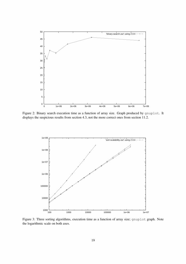
plot ’binary-search.out’ using 2:3:4 with errorlines

This says that the data (x, y, dy) are in columns 2, 3 and 4 (thus ignoring the descriptive text in column

1) of text file binary-search.out, and that dy should be used for plotting y-value error bars at

each data point (x, y). The resulting plot is shown in figure 2.

Similarly, we can plot the running times of the three sorting algorithms benchmarked in section 6,

using logarithmic axes because selection sort is so much slower than quicksort and heap sort:

set term postscript

set output "sorting-plot.ps"

set logscale xy

plot ’sort-scalability.out’ using 2:3:4 with errorlines

The resulting plot is shown in figure 3. Gnuplot has many options and features, see its manual.

10 Simple charting with Excel

In MS Excel 2010 or 2013 for Windows, choose File > Open > All Files and select a text

output file such as that created in section 4.3. A Text Import Wizard dialog appears, where you should

choose Fixed width, and may choose Start import at row 5 (to ignore the system infor-

mation at the top of the file), then click Next. The wizard will usually guess the columns correctly, in

which case just click Next again, then Finish. In Excel 2011 for Mac, choose File > Import

> Text file > Import > All files and select the appropriate text file, to get a similar Text

Import Wizard. Hint: If Excel uses decimal comma and the text file uses decimal point, or vice versa,

then open the Advanced subdialog and change Excel’s expectations; otherwise the import goes wrong.

The data appears in an Excel sheet, as shown in figure 4.

18

0

5

10

15

20

25

30

35

40

45

50

0 1e+06 2e+06 3e+06 4e+06 5e+06 6e+06 7e+06

’binary-search.out’ using 2:3:4

Figure 2: Binary search execution time as a function of array size. Graph produced by gnuplot. It

displays the suspicious results from section 4.3, not the more correct ones from section 11.2.

1000

10000

100000

1e+06

1e+07

1e+08

1e+09

100 1000 10000 100000 1e+06 1e+07

’sort-scalability.out’ using 2:3:4

Figure 3: Three sorting algorithms, execution time as a function of array size; gnuplot graph. Note

the logarithmic scale on both axes.

19

Figure 4: Binary search execution time data imported into Excel 2013.

To display this kind of data, one should almost always use a scatter plot (xy-plot), not any of the other

fancy but more business-oriented chart types. Select the data in columns B and C, that is, range B1:C17,

as shown in the figure, choose Insert > Charts > Scatter, and choose the chart subtype with

straight lines and markers. Smooth lines may look neater, but they distort the data. The result will be a

chart as shown in figure 5. The appearance of such charts can be improved interactively by right-clicking

on relevant chart elements, such as the axes, the plot lines, the data point markers, chart background,

and so on.

Figure 5: Excel scatter chart showing the binary search data from figure 4.

20

11 Benchmark design considerations

Until now we have mostly been concerned with how to measure execution time. We also need to think

about what to measure: on which inputs should we run the code when measuring execution time? The

answer of course is highly problem dependent, but for inspiration, let us consider again the binary search

benchmark.

11.1 Benchmark design for binary search

The binary search routine in section 4.3 has two input parameters whose values we need to choose: the

item x to search for, and the sorted array arr of items to search in.

• Let us consider first the array arr. It is clear that the execution time depends on the size of the

array, so we want to call the method on a range of such sizes. Indeed we did that, by virtue of the

outer for loop, in section 4.3.

The array should be sorted in non-decreasing order (or else the method does not work at all), but

still there are many possible choices of array contents: all items are equal, some items are equal,

or no items are equal (that is, all items are distinct). For binary search, the latter choice forces

the worst case execution time, so that is what we choose. Moreover, when all items are distinct,

they may be dense as in 0, 1, 2, 3, . . . or have gaps as in 1, 17, 18, 23, . . .. For the execution time

of binary search in a sorted array, this makes no difference, but for other representations of sets or

bags it may. We choose a dense set of items.

• Next, what items x should we search for? The most basic decision is whether we want successful

search (for an item that is in the array) or an unsuccessful search (for an item not in the array).

The latter forces the highest execution time, and therefore might be a reasonable choice, but

precisely for binary search it does not make much of a difference. In general one should choose a

representative mix of successful and unsuccessful searches.

In the example from section 4.3, we ran only successful searches, and always for the same item

successItem, at a position just before the middle of the array. In retrospect, this was a dubious

choice, because the same search is performed repeatedly and each one will hit the same array

positions, which are therefore almost guaranteed to be in all levels of CPU caches. This unrealistic

scenario may severely underestimate the typical execution time for a successful binary search.

There are several ways to remedy this situation. For an n-element array, we could either search

for the items 0, 1, ..., n − 1 in order, or we could repeatedly generate a pseudorandom number in

the range [0, n − 1] and search for that. However, the first approach is “too predictable”, likely to

use the caches well, and hence report unrealistically low execution times. The second approach

suffers from another problem: the cost of generating a pseudorandom item to search for is high,

comparable to that of the search itself. We will investigate this and a possible solution in the next

section.

11.2 Binary search for pseudorandom items

We can generate a pseudorandom item in the range [0, n − 1] by rnd.nextInt(n). Using the ma-

chinery already developed we can measure the cost of this operation:

final java.util.Random rnd = new java.util.Random();

final int n = 1638400;

Mark8("random_index", i -> rnd.nextInt(n));

21

Running this code tells us that the cost of generating a pseudorandom item is a whopping 12.0 ns, which

is comparable to be cost of the binary search itself as measured in section 4.3. Even when searching

an array with millions of items, this is nearly a quarter of the cost of the search itself, and thus would

seriously distort the measurements.

What can be done? One possibility is to pre-generate a large enough array items of pseudorandom

items before performing the benchmark, and sequentially retrieve and search for these items in the

benchmark itself. Then the time measurements will include the time to access the items array, but

this access will be sequential and cache-friendly, and hence hopefully not contribute too much to the

execution time:


final int[] intArray = SearchAndSort.fillIntArray(size); // sorted [0,1,...]

final int[] items = SearchAndSort.fillIntArray(size);

final int n = size;

SearchAndSort.shuffle(items);

Mark8("binary_search_success",


i -> SearchAndSort.binarySearch(items[i % n], intArray));

}

Now the results are as follows:


















These execution times are up to 7 times higher than those measured in section 4.3! Whether they are

more correct is a question of which usage scenario is more likely in practice: repeatedly searching for

the same item, or repeatedly searching for an item that is completely unrelated to the one previously

searched for. Certainly the latter gives a more conservative execution time estimate, and one that fits the

textbook complexity O(log n) for binary search better.

Note that we still perform only successful searches, which may be unrealistic. To improve on this

situation we could make the intArray contain only odd numbers 1, 3, 5, . . . and have both even and

odd numbers in the array of items to search for. It is left as an exercise to see what results this would

give.

Another possible concern is that the new higher execution times include the time to compute the

remainder operator (%) and retrieve the pre-generated pseudorandom items from the array. If we suspect

that this overhead is significant, we can measure it:

22


final int[] items = SearchAndSort.fillIntArray(size);

final int n = size;

SearchAndSort.shuffle(items);

Mark8("get_pseudorandom_items",


i -> items[i % n]);

}

The results below show that the time to access the pseudorandom items is quite negligible, and com-

pletely constant over very different items array sizes, confirming that the sequential retrieval of items

is cache-friendly:

get_pseudorandom_items 100 6.9 0.07 67108864

















12 Source code for examples

The complete source code presented here, including the examples, can be found (in Java and C#) at:

http://www.itu.dk/people/sestoft/javaprecisely/benchmarks-java.zip

http://www.itu.dk/people/sestoft/csharpprecisely/benchmarks-csharp.zip

The hope is that the reader can adapt and further develop the benchmarking code to any particular use

context.

13 Other online resources

• Brent Boyer: Robust Java benchmarking, Part 1: Issues and Part 2: Statistics and solutions [1].

• Cliff Click: How NOT to write a microbenchmark [2].

• Brian Goetz: Java theory and practice: Dynamic compilation and performance measurement [3].

• Brian Goetz: Java theory and practice: Anatomy of a flawed microbenchmark [4].

• TODO: ... more

23

14 Acknowledgements

Thanks to the many students whose unexpected benchmark results inspired this note; to Finn Schiermer

Andersen and David Christiansen for helping explain unreasonable results in C and Scala; to Claus

Brabrand for suggestions that led to big improvements in the presentation; and to Kasper Østerbye,

Michael Reichhardt Hansen for constructive comments on drafts.

15 Exercises

Exercise 1: Run the Mark1 through Mark6measurements yourself. Use the SystemInfomethod to

record basic system identification, and supplement with whatever other information you can find about

the execution platform; see section 8.

Exercise 2: Use Mark7 to measure the execution time for the mathematical functions pow, exp, and

so on, as in section 4.2. Record the results along with appropriate system identification. Preferably do

this on at least two different platforms, eg. your own computer and a fellow student’s or a computer at

the university.

Exercise 3: Run the measurements of sorting algorithm performance as in section 6. Record the results

along with appropriate system identification. Use Excel or gnuplot or some other charting package to

make graphs of the execution time as function of the problem size, as in figure 3. Preferably do this

on at least two different platforms, eg. your own computer and a fellow student’s or a computer at the

university.

Appendix: Tips from the creators of the Hotspot JVM

Below are some tips about writing micro benchmarks for the Sun/Oracle HotSpot Java Virtual Machine,

reproduced from [5]. While the advice is of general interest, the runtime options of type -X and -XX

discussed below are non-standard. They are subject to change at any time and not guaranteed to work

on, say, IBM or Apple implementations of the Java Virtual Machine.

• Rule 0: Read a reputable paper on JVMs and micro-benchmarking. A good one is Brian Goetz,

2005 [4]. Do not expect too much from micro-benchmarks; they measure only a limited range of

JVM performance characteristics.

• Rule 1: Always include a warmup phase which runs your test kernel all the way through, enough

to trigger all initializations and compilations before timing phase(s). (Fewer iterations is OK on

the warmup phase. The rule of thumb is several tens of thousands of inner loop iterations.)

• Rule 2: Always run with -XX:+PrintCompilation, -verbose:gc, etc., so you can verify that the

compiler and other parts of the JVM are not doing unexpected work during your timing phase.

• Rule 2.1: Print messages at the beginning and end of timing and warmup phases, so you can verify

that there is no output from Rule 2 during the timing phase.

• Rule 3: Be aware of the difference between -client and -server, and OSR [On-Stack Replacement]

and regular compilations. The -XX:+PrintCompilation flag reports OSR compilations with an

at-sign to denote the non-initial entry point, for example: Trouble$1::run @ 2 (41 bytes). Prefer

server to client, and regular to OSR, if you are after best performance.

• Rule 4: Be aware of initialization effects. Do not print for the first time during your timing phase,

since printing loads and initializes classes. Do not load new classes outside of the warmup phase

24

(or final reporting phase), unless you are testing class loading specifically (and in that case load

only the test classes). Rule 2 is your first line of defense against such effects.

• Rule 5: Be aware of deoptimization and recompilation effects. Do not take any code path for the

first time in the timing phase, because the compiler may junk and recompile the code, based on an

earlier optimistic assumption that the path was not going to be used at all. Rule 2 is your first line

of defense against such effects.

• Rule 6: Use appropriate tools to read the compiler’s mind, and expect to be surprised by the code

it produces. Inspect the code yourself before forming theories about what makes something faster

or slower.

• Rule 7: Reduce noise in your measurements. Run your benchmark on a quiet machine, and run it

several times, discarding outliers. Use -Xbatch to serialize the compiler with the application, and

consider setting -XX:CICompilerCount=1 to prevent the compiler from running in parallel with

itself.

Similar tips would apply to the Common Language Infrastructure (.NET) platform, but the Microsoft

.NET implementation does not seem to have (publicly available) means for controlling just-in-time com-

pilation and so on. Only the choice of garbage collector can be controlled, using the runtime settings

schema of the so-called application configuration files, named MyApp.exe.config or similar. I

have no experience with this. The Mono implementation has a range of runtime configuration options,

displayed by mono -help and mono -list-opt.

References

[1] Brent Boyer: Robust Java benchmarking, Part 1: Issues and Part 2: Statistics and solutions. IBM

developerWorks, 24 June 2008, at

http://www.ibm.com/developerworks/java/library/j-benchmark1/ and

http://www.ibm.com/developerworks/java/library/j-benchmark2/

[2] Cliff Click: How NOT to write a microbenchmark. JavaOne 2002 talk, at

http://www.azulsystems.com/events/javaone_2002/microbenchmarks.pdf

[3] Brian Goetz: Java theory and practice: Dynamic compilation and performance measurement. IBM

developerWorks, 21 December 2004, at

http://www.ibm.com/developerworks/library/j-jtp12214/

[4] Brian Goetz: Java theory and practice: Anatomy of a flawed microbenchmark. IBM developer-

Works, 22 February 2005, at

http://www.ibm.com/developerworks/java/library/j-jtp02225/index.html

[5] John Rose: Microbenchmarks: So You Want to Write a Micro-Benchmark HotSpot Internals wiki,

at https://wikis.oracle.com/display/HotSpotInternals/MicroBenchmarks

[6] Scala documentation: Parallel Collections: Measuring Performance Scala documentation page, at

http://docs.scala-lang.org/overviews/parallel-collections/performance.html

25

microbenchmarks in java and c#sestoft/papers/benchmarking.pdf · 2015-09-16 · microbenchmarks in...

Documents