mid-permian cyclothem development in the onshore canning ...mid-permian cyclothem development in the...
TRANSCRIPT
This file is part of the following reference:
Adkins, Rhonda Michelle (2003) Mid-Permian cyclothem
development in the onshore Canning Basin, Western
Australia. PhD thesis, James Cook University.
Access to this file is available from:
http://researchonline.jcu.edu.au/1345/
If you believe that this work constitutes a copyright infringement, please contact
[email protected] and quote http://researchonline.jcu.edu.au/1345/
ResearchOnline@JCU
Mid-Permian cyclothem development in the onshore CanningBasin, Western Australia
Volume I
Thesis submitted by
Rhonda Michelle Adkins (M.S. Virginia Tech)
in May 2003
for the degree of Doctor of Philosophy
in the School of Earth Sciences
James Cook University of North Queensland, Australia
PhD Thesis Adkins, Access
ii
Statement of Access
I, the undersigned author of this thesis, understand that James Cook University will
make this thesis available for use within the University Library and, by microfilm or
other means, allow access to other users in other approved libraries.
All users consulting this thesis will have to sign the following statement:
In consulting this thesis I agree not to copy closely or paraphrase it in whole or
in part without the written consent of the author; and to make proper public
written acknowledgment for any assistance that I have obtained from it.
Beyond this, I do not wish to place any restrictions on access to this thesis.
Rhonda M. Adkins May 2003
PhD Thesis Adkins, Access
iii
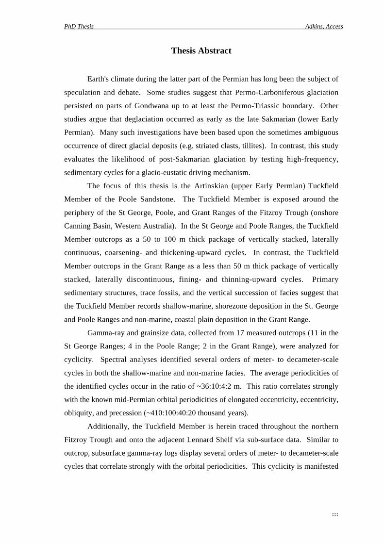
Thesis Abstract
Earth's climate during the latter part of the Permian has long been the subject of
speculation and debate. Some studies suggest that Permo-Carboniferous glaciation
persisted on parts of Gondwana up to at least the Permo-Triassic boundary. Other
studies argue that deglaciation occurred as early as the late Sakmarian (lower Early
Permian). Many such investigations have been based upon the sometimes ambiguous
occurrence of direct glacial deposits (e.g. striated clasts, tillites). In contrast, this study
evaluates the likelihood of post-Sakmarian glaciation by testing high-frequency,
sedimentary cycles for a glacio-eustatic driving mechanism.
The focus of this thesis is the Artinskian (upper Early Permian) Tuckfield
Member of the Poole Sandstone. The Tuckfield Member is exposed around the
periphery of the St George, Poole, and Grant Ranges of the Fitzroy Trough (onshore
Canning Basin, Western Australia). In the St George and Poole Ranges, the Tuckfield
Member outcrops as a 50 to 100 m thick package of vertically stacked, laterally
continuous, coarsening- and thickening-upward cycles. In contrast, the Tuckfield
Member outcrops in the Grant Range as a less than 50 m thick package of vertically
stacked, laterally discontinuous, fining- and thinning-upward cycles. Primary
sedimentary structures, trace fossils, and the vertical succession of facies suggest that
the Tuckfield Member records shallow-marine, shorezone deposition in the St. George
and Poole Ranges and non-marine, coastal plain deposition in the Grant Range.
Gamma-ray and grainsize data, collected from 17 measured outcrops (11 in the
St George Ranges; 4 in the Poole Range; 2 in the Grant Range), were analyzed for
cyclicity. Spectral analyses identified several orders of meter- to decameter-scale
cycles in both the shallow-marine and non-marine facies. The average periodicities of
the identified cycles occur in the ratio of ~36:10:4:2 m. This ratio correlates strongly
with the known mid-Permian orbital periodicities of elongated eccentricity, eccentricity,
obliquity, and precession (~410:100:40:20 thousand years).
Additionally, the Tuckfield Member is herein traced throughout the northern
Fitzroy Trough and onto the adjacent Lennard Shelf via sub-surface data. Similar to
outcrop, subsurface gamma-ray logs display several orders of meter- to decameter-scale
cycles that correlate strongly with the orbital periodicities. This cyclicity is manifested
PhD Thesis Adkins, Access
iv
by the systematic bundling of smaller-scale cycles into larger-scale cycles that can be
traced laterally for more than 200 km.
For comparison, correlative shallow-marine cycles from the Artinskian to
Ufimian Pebbley Beach Formation (Sydney Basin, New South Wales) were also
studied. Four outcrop sections were measured and correlated, giving a total
stratigraphic column of approximately 45 m. Spectral analysis of gamma-ray data
identified several orders of meter- to decameter-scale cycles. These cycles correlate
strongly with the mid-Permian orbital periodicities and the identified Tuckfield Member
cycles.
The favorable comparison between the Tuckfield Member cycles and the orbital
parameters indicates that Milankovitch-forcing of climate influenced the formation of
depositional cyclicity. Furthermore, it is highly probable that these cycles are glacio-
eustatic in origin due to their laterally extensive nature and positive correlation with
identified cyclicity in New South Wales. This suggests that Permo-Carboniferous
glaciation must have persisted into at least the Ufimian stage of the Late Permian.
PhD Thesis Adkins, Access
v
Acknowledgments
This project benefited from the assistance and support of many people and
professional organizations. The research was funded by the Australian Research
Council, the American Association of Petroleum Geologists, and the Society of
Professional Well Log Analysts. Additional support was provided by James Cook
University in the form of an International Postgraduate Research Scholarship and a
School of Earth Sciences Scholarship. The Petroleum Exploration Society of Australia,
the Geological Society of Australia, and the Australasian Sedimentologists Group (all of
whom provided grants to attend professional conferences) are gratefully acknowledged
for their support.
The Geological Survey of Western Australia is also thanked for its advice and
assistance. At the survey, Neil Apak and Rosie Emms provided much appreciated
geological and logistical help. At James Cook University, the Advanced Analytical
Center assisted with the collection of geochemical data. Additionally, Graham Weedon
is thanked for providing a copy of his spectral analysis program to our research group.
Thanks are also given to Phil Playford and Albert Brakel who reviewed the manuscript
associated with Chapter 1. The entire thesis was much improved by their constructive
comments. In the Canning Basin, the Kimberley Land Council, local aboriginal
communities, and local station owners/managers are gratefully acknowledged for land
access and assistance in the field.
I would also like to acknowledge many people in the School of Earth Sciences at
James Cook University. I greatly appreciate the assistance that I received from
departmental staff members (especially Melissa Thomson, Rachel Mahon, Kevin
Hooper, and Paul Givney). As a post-doc, Steve Abbott inspired this project before
moving on to bigger and better things. Helen Lever assisted with fieldwork in New
South Wales and generally acted as an empathetic sounding board for this work.
Members of the Marine Group and Samri provided much appreciated advice, support,
and companionship. Keith Crook and Peter Crosdale are especially noted for their
geological help. People in my office block (particularly Mike Page), Cameron
Huddlestone-Holmes (and Laurene), Tom Evans (and Rachel), and Katharine Grant are
especially noted for their friendship and general support.
PhD Thesis Adkins, Access
vi
Of course, my biggest thanks go to my advisor, Bob Carter. In addition to
providing geological/professional guidance, Bob also supplied financial and (sometimes
much needed) emotional support. During the past three years, I have come to realize
that Bob is not only a superb geologist but also a fair, forward-thinking, and extremely
generous man. I consider myself fortunate to have had the opportunity to study under
his tutelage.
Finally, I would like to thank my friends and family in the USA. There are no words
to describe how much I appreciated their support and encouragement during my time in
Australia. I also give a huge, heart-felt thanks to Peter Welch: my field assistant,
computer technician, personal chef, dear friend, and most cherished love. He has been
my source of sanity throughout everything, and none of this would have been possible
without his unending support.
PhD Thesis Adkins, Access
vii
Table of Contents
Volume I
Thesis Abstract . . . . . . . . . . . . . . . . . . . . . . . iii
Acknowledgments . . . . . . . . . . . . . . . . . . . . . . v
List of Figures. . . . . . . . . . . . . . . . . . . . . . . . xi
List of Tables . . . . . . . . . . . . . . . . . . . . . . . . xiv
Preface
Mid-Permian cyclothem development in the onshore Canning Basin,
Western Australia: project overview and thesis details . . . . . . . . . . 1
Introduction . . . . . . . . . . . . . . . . . . . . . . . 2
Project Details. . . . . . . . . . . . . . . . . . . . . . . 2
Thesis Format and Chapter Summaries . . . . . . . . . . . . . . 3
Chapter 1
Regressive systems tract cyclici ty in shorezone deposits: the
sedimentology and stratigraphy of the Early Permian Tuckfield Member
(Poole Sandstone), onshore Canning Basin, Western Australia . . . . . . . 7
Abstract . . . . . . . . . . . . . . . . . . . . . . . . 8
Key Words . . . . . . . . . . . . . . . . . . . . . . . . 8
Introduction . . . . . . . . . . . . . . . . . . . . . . . 8
Methods . . . . . . . . . . . . . . . . . . . . . . . . 11
Regional Setting and Depositional History . . . . . . . . . . . . . 15
The Tuckfield Member of the Poole Sandstone . . . . . . . . . . . . 17
Cycle Model . . . . . . . . . . . . . . . . . . . . . . 17
Detailed Cycle Analyses . . . . . . . . . . . . . . . . . . 22
Petrography . . . . . . . . . . . . . . . . . . . . . 25
Geochemistry . . . . . . . . . . . . . . . . . . . . . 25
Depositional Environment. . . . . . . . . . . . . . . . . . . 25
Sequence Stratigraphic Framework. . . . . . . . . . . . . . . . 29
Conclusions . . . . . . . . . . . . . . . . . . . . . . 32
PhD Thesis Adkins, Access
viii
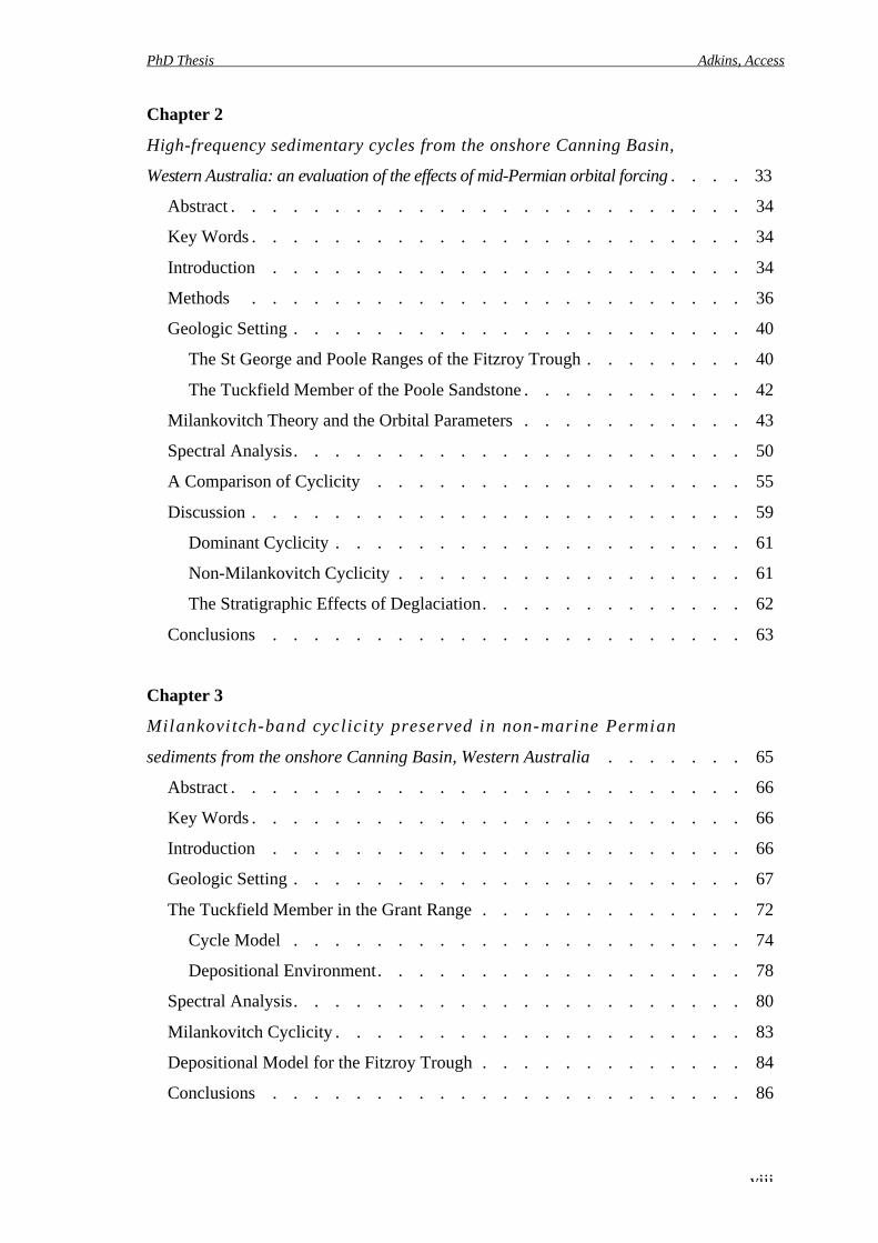
Chapter 2
High-frequency sedimentary cycles from the onshore Canning Basin,
Western Australia: an evaluation of the effects of mid-Permian orbital forcing . . . . 33
Abstract . . . . . . . . . . . . . . . . . . . . . . . . . 34
Key Words . . . . . . . . . . . . . . . . . . . . . . . . 34
Introduction . . . . . . . . . . . . . . . . . . . . . . . 34
Methods . . . . . . . . . . . . . . . . . . . . . . . . 36
Geologic Setting . . . . . . . . . . . . . . . . . . . . . . 40
The St George and Poole Ranges of the Fitzroy Trough . . . . . . . . 40
The Tuckfield Member of the Poole Sandstone . . . . . . . . . . . 42
Milankovitch Theory and the Orbital Parameters . . . . . . . . . . . 43
Spectral Analysis. . . . . . . . . . . . . . . . . . . . . . 50
A Comparison of Cyclicity . . . . . . . . . . . . . . . . . . 55
Discussion . . . . . . . . . . . . . . . . . . . . . . . . 59
Dominant Cyclicity . . . . . . . . . . . . . . . . . . . . 61
Non-Milankovitch Cyclicity . . . . . . . . . . . . . . . . . 61
The Stratigraphic Effects of Deglaciation. . . . . . . . . . . . . 62
Conclusions . . . . . . . . . . . . . . . . . . . . . . . 63
Chapter 3
Milankovi tch-band cyclicity preserved in non-marine Permian
sediments from the onshore Canning Basin, Western Australia . . . . . . . 65
Abstract . . . . . . . . . . . . . . . . . . . . . . . . . 66
Key Words . . . . . . . . . . . . . . . . . . . . . . . . 66
Introduction . . . . . . . . . . . . . . . . . . . . . . . 66
Geologic Setting . . . . . . . . . . . . . . . . . . . . . . 67
The Tuckfield Member in the Grant Range . . . . . . . . . . . . . 72
Cycle Model . . . . . . . . . . . . . . . . . . . . . . 74
Depositional Environment. . . . . . . . . . . . . . . . . . 78
Spectral Analysis. . . . . . . . . . . . . . . . . . . . . . 80
Milankovitch Cyclicity . . . . . . . . . . . . . . . . . . . . 83
Depositional Model for the Fitzroy Trough . . . . . . . . . . . . . 84
Conclusions . . . . . . . . . . . . . . . . . . . . . . . 86
PhD Thesis Adkins, Access
ix
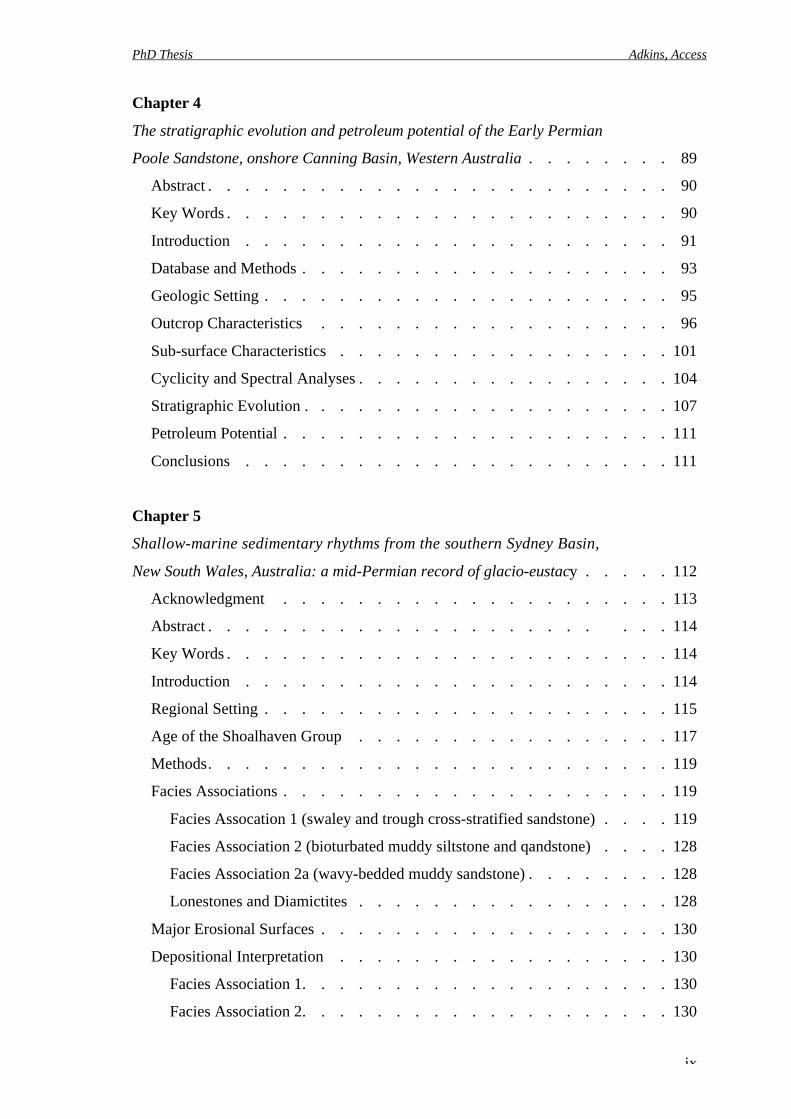
Chapter 4
The stratigraphic evolution and petroleum potential of the Early Permian
Poole Sandstone, onshore Canning Basin, Western Australia . . . . . . . . 89
Abstract . . . . . . . . . . . . . . . . . . . . . . . . . 90
Key Words . . . . . . . . . . . . . . . . . . . . . . . . 90
Introduction . . . . . . . . . . . . . . . . . . . . . . . 91
Database and Methods . . . . . . . . . . . . . . . . . . . . 93
Geologic Setting . . . . . . . . . . . . . . . . . . . . . . 95
Outcrop Characteristics . . . . . . . . . . . . . . . . . . . 96
Sub-surface Characteristics . . . . . . . . . . . . . . . . . . 101
Cyclicity and Spectral Analyses . . . . . . . . . . . . . . . . . 104
Stratigraphic Evolution . . . . . . . . . . . . . . . . . . . . 107
Petroleum Potential . . . . . . . . . . . . . . . . . . . . . 111
Conclusions . . . . . . . . . . . . . . . . . . . . . . . 111
Chapter 5
Shallow-marine sedimentary rhythms from the southern Sydney Basin,
New South Wales, Australia: a mid-Permian record of glacio-eustacy . . . . . 112
Acknowledgment . . . . . . . . . . . . . . . . . . . . . 113
Abstract . . . . . . . . . . . . . . . . . . . . . . . . 114
Key Words . . . . . . . . . . . . . . . . . . . . . . . . 114
Introduction . . . . . . . . . . . . . . . . . . . . . . . 114
Regional Setting . . . . . . . . . . . . . . . . . . . . . . 115
Age of the Shoalhaven Group . . . . . . . . . . . . . . . . . 117
Methods. . . . . . . . . . . . . . . . . . . . . . . . . 119
Facies Associations . . . . . . . . . . . . . . . . . . . . . 119
Facies Assocation 1 (swaley and trough cross-stratified sandstone) . . . . 119
Facies Association 2 (bioturbated muddy siltstone and qandstone) . . . . 128
Facies Association 2a (wavy-bedded muddy sandstone) . . . . . . . . 128
Lonestones and Diamictites . . . . . . . . . . . . . . . . . 128
Major Erosional Surfaces . . . . . . . . . . . . . . . . . . . 130
Depositional Interpretation . . . . . . . . . . . . . . . . . . 130
Facies Association 1. . . . . . . . . . . . . . . . . . . . 130
Facies Association 2. . . . . . . . . . . . . . . . . . . . 130
PhD Thesis Adkins, Access
x
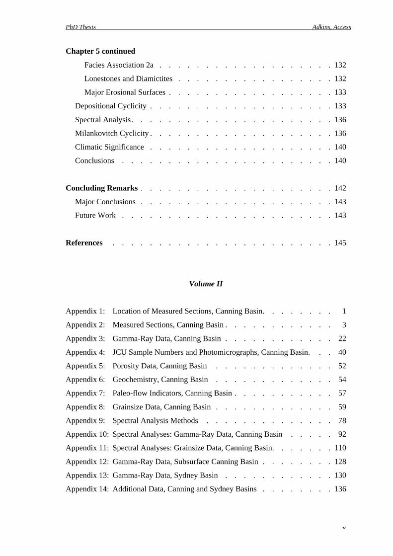
Chapter 5 continued
Facies Association 2a . . . . . . . . . . . . . . . . . . . 132
Lonestones and Diamictites . . . . . . . . . . . . . . . . . 132
Major Erosional Surfaces . . . . . . . . . . . . . . . . . . 133
Depositional Cyclicity . . . . . . . . . . . . . . . . . . . . 133
Spectral Analysis. . . . . . . . . . . . . . . . . . . . . . 136
Milankovitch Cyclicity . . . . . . . . . . . . . . . . . . . . 136
Climatic Significance . . . . . . . . . . . . . . . . . . . . 140
Conclusions . . . . . . . . . . . . . . . . . . . . . . . 140
Concluding Remarks . . . . . . . . . . . . . . . . . . . . . 142
Major Conclusions . . . . . . . . . . . . . . . . . . . . . 143
Future Work . . . . . . . . . . . . . . . . . . . . . . . 143
References . . . . . . . . . . . . . . . . . . . . . . . . 145
Volume II
Appendix 1: Location of Measured Sections, Canning Basin. . . . . . . . 1
Appendix 2: Measured Sections, Canning Basin . . . . . . . . . . . . 3
Appendix 3: Gamma-Ray Data, Canning Basin . . . . . . . . . . . . 22
Appendix 4: JCU Sample Numbers and Photomicrographs, Canning Basin. . . 40
Appendix 5: Porosity Data, Canning Basin . . . . . . . . . . . . . 52
Appendix 6: Geochemistry, Canning Basin . . . . . . . . . . . . . 54
Appendix 7: Paleo-flow Indicators, Canning Basin . . . . . . . . . . . 57
Appendix 8: Grainsize Data, Canning Basin . . . . . . . . . . . . . 59
Appendix 9: Spectral Analysis Methods . . . . . . . . . . . . . . 78
Appendix 10: Spectral Analyses: Gamma-Ray Data, Canning Basin . . . . . 92
Appendix 11: Spectral Analyses: Grainsize Data, Canning Basin. . . . . . . 110
Appendix 12: Gamma-Ray Data, Subsurface Canning Basin . . . . . . . . 128
Appendix 13: Gamma-Ray Data, Sydney Basin . . . . . . . . . . . . 130
Appendix 14: Additional Data, Canning and Sydney Basins . . . . . . . . 136
PhD Thesis Adkins, Access
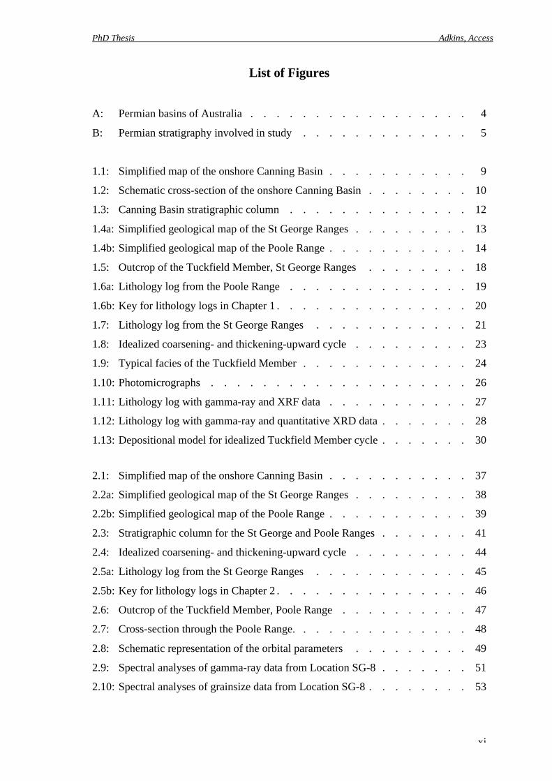
xi
List of Figures
A: Permian basins of Australia . . . . . . . . . . . . . . . . . 4
B: Permian stratigraphy involved in study . . . . . . . . . . . . . 5
1.1: Simplified map of the onshore Canning Basin . . . . . . . . . . . 9
1.2: Schematic cross-section of the onshore Canning Basin . . . . . . . . 10
1.3: Canning Basin stratigraphic column . . . . . . . . . . . . . . 12
1.4a: Simplified geological map of the St George Ranges . . . . . . . . . 13
1.4b: Simplified geological map of the Poole Range . . . . . . . . . . . 14
1.5: Outcrop of the Tuckfield Member, St George Ranges . . . . . . . . 18
1.6a: Lithology log from the Poole Range . . . . . . . . . . . . . . 19
1.6b: Key for lithology logs in Chapter 1 . . . . . . . . . . . . . . . 20
1.7: Lithology log from the St George Ranges . . . . . . . . . . . . 21
1.8: Idealized coarsening- and thickening-upward cycle . . . . . . . . . 23
1.9: Typical facies of the Tuckfield Member . . . . . . . . . . . . . 24
1.10: Photomicrographs . . . . . . . . . . . . . . . . . . . . 26
1.11: Lithology log with gamma-ray and XRF data . . . . . . . . . . . 27
1.12: Lithology log with gamma-ray and quantitative XRD data . . . . . . . 28
1.13: Depositional model for idealized Tuckfield Member cycle . . . . . . . 30
2.1: Simplified map of the onshore Canning Basin . . . . . . . . . . . 37
2.2a: Simplified geological map of the St George Ranges . . . . . . . . . 38
2.2b: Simplified geological map of the Poole Range . . . . . . . . . . . 39
2.3: Stratigraphic column for the St George and Poole Ranges . . . . . . . 41
2.4: Idealized coarsening- and thickening-upward cycle . . . . . . . . . 44
2.5a: Lithology log from the St George Ranges . . . . . . . . . . . . 45
2.5b: Key for lithology logs in Chapter 2 . . . . . . . . . . . . . . . 46
2.6: Outcrop of the Tuckfield Member, Poole Range . . . . . . . . . . 47
2.7: Cross-section through the Poole Range. . . . . . . . . . . . . . 48
2.8: Schematic representation of the orbital parameters . . . . . . . . . 49
2.9: Spectral analyses of gamma-ray data from Location SG-8 . . . . . . . 51
2.10: Spectral analyses of grainsize data from Location SG-8 . . . . . . . . 53

PhD Thesis Adkins, Access
xii
3.1: Simplified map of the onshore Canning Basin . . . . . . . . . . . 68
3.2: Early Permian stratigraphic column for the Fitzroy Trough . . . . . . . 69
3.3: Simplified geological map of the Grant Range . . . . . . . . . . . 70
3.4: Early Permian (Sakmarian) paleo-geographic reconstruction . . . . . . 71
3.5: Typical outcrops of the Tuckfield Member . . . . . . . . . . . . 73
3.6a: Lithology log from the Grant Range . . . . . . . . . . . . . . 75
3.6b: Key for lithology log in Chapter 3 . . . . . . . . . . . . . . . 76
3.7: Shallow-marine and non-marine cycle models, Tuckfield Member . . . . 77
3.8: Mud pellets and sandstone clasts typical of non-marine Tuckfield sediments . 79
3.9: Spectral analyses of gamma-ray data from Location G-1 . . . . . . . 81
3.10: Spectral analyses of gamma-ray data from Location G-2 . . . . . . . 82
3.11: Simplified depositional model for the mid-Permian Fitzroy Trough . . . . 87
4.1: Simplified map of the Fitzroy Trough . . . . . . . . . . . . . . 92
4.2: Early Permian stratigraphic column for the Fitzroy Trough . . . . . . . 97
4.3a Comparison of outcrop and sub-surface stratigraphy . . . . . . . . . 98
4.3b Key for lithology log in Chapter 4 . . . . . . . . . . . . . . . 99
4.4: Outcrop of the Tuckfield Member, Poole Range . . . . . . . . . . 100
4.5 Sub-surface gamma-ray log, Sundown 2 . . . . . . . . . . . . . 102
4.6 Sub-surface cross-section, approximately perpendicular to strike . . . . . 103
4.7 Tuckfield Member isopach map . . . . . . . . . . . . . . . . 105
4.8 Sub-surface cross-section, approximately parallel to strike . . . . . . . 106
4.9 Spectral analyses of gamma-ray data from Terrace 1 . . . . . . . . . 108
5.1: Simplified map of the southern Sydney Basin . . . . . . . . . . . 116
5.2: Stratigraphic units of the southern Sydney Basin . . . . . . . . . . 118
5.3a: Lithology log from Point Upright . . . . . . . . . . . . . . . 120
5.3b: Key for lithology logs in Chapter 5 . . . . . . . . . . . . . . . 121
5.4: Lithology log from south of Pebbly Beach . . . . . . . . . . . . 122
5.5: Lithology log from Mill Point . . . . . . . . . . . . . . . . 123
5.6: Lithology log from Clear Point . . . . . . . . . . . . . . . . 124
5.7: Correlation of Pebbley Beach sections. . . . . . . . . . . . . . 125
5.8: Composite Pebbley Beach lithology log . . . . . . . . . . . . . 126
5.9: Typical facies from the Pebbley Beach Formation . . . . . . . . . . 127

PhD Thesis Adkins, Access
xiii
5.10: Ice-rafted debris . . . . . . . . . . . . . . . . . . . . . 129
5.11: Erosional surface at Mill Point . . . . . . . . . . . . . . . . 131
5.12: Cycles at Point Upright. . . . . . . . . . . . . . . . . . . 134
5.13: Idealized cycle model, Pebbley Beach Formation . . . . . . . . . . 135
5.14: Spectral analyses of gamma-ray data from composite Pebbley Beach section . 137
PhD Thesis Adkins, Access
xiv
List of Tables
2.1: Detected Tuckfield Member cycles, St George and Poole Ranges. . . . . 54
2.2: Computed Tuckfield Member cycle ratios (gamma-ray data) . . . . . . 56
2.3: Computed Tuckfield Member cycle ratios (grainsize data) . . . . . . . 57
2.4: Comparision of shallow-marine cycles with Milankovitch periodicities. . . 58
2.5: Global comparison of post-Sakmarian shallow-marine cycles . . . . . . 60
3.1: Comparison of non-marine Tuckfield Member cycles with shallow-
marine Tuckfield Member cycles and Milankovitch periodicities . . . . . 85
4.1: Well data, northern Fitzroy Trough . . . . . . . . . . . . . . . 94
5.1: Comparison of Pebbley Beach cycles with Milankovitch periodicities . . . 139
PhD Thesis Adkins, Access
xv
Statement of Sources
Declaration
I declare that this thesis is my own work and has not been submitted in any form for
another degree or diploma at any university or other institute of tertiary education.
Information derived from the published or unpublished work of others has been
acknowledged in the text and a list of references is given.
Rhonda M. Adkins May 2003
PhD Thesis Adkins, Preface
1
Preface
Mid-Permian cyclothem development in the onshoreCanning Basin, Western Australia: project overview and
thesis details
PhD Thesis Adkins, Preface
2
INTRODUCTION
The Permian was a period of significant climatic change. During that time, the
late Paleozoic ice age reached its climax, waned, and eventually gave way to global
greenhouse conditions (Crowell, 1978). Similar to the Permo-Carboniferous, Earth's
climate during the past 35 million years has been characterized by alternating glacial
(colder) and interglacial (warmer) phases (e.g. Dickens, 1996; Zachos et al., 2001). As
occurred during the late Paleozoic, it can be expected that today's glaciers will
eventually retreat and again give way to global greenhouse conditions. For this reason,
it is important for us to gain a better understanding of Earth's climatic evolution during
the Permian. By doing so, we may obtain valuable insight into Earth's present climatic
systems and be able to better predict future climatic variations.
Today, it is widely accepted that the earliest Permian was marked by widespread
glaciation. Likewise, it is equally accepted that, by the earliest Triassic, global
greenhouse conditions prevailed. However, Earth's climate during the transitional
period between the earliest Permian and the earliest Triassic remains the subject of
much speculation. Evidence suggests that glacial retreat began during the Sakmarian
stage of the Early Permian (Dickens, 1996), but exactly how long glaciation continued
past this point is debatable. Some believe that there is strong evidence in Australia that
glaciation may have persisted up to the Triassic boundary (Veevers, 2000a). However,
others suggest that Gondwanan deglaciation and the onset of global greenhouse
conditions occurred by the end of the Early Permian (Visser, 1993a; von Brun, 1996).
Some have even argued that Gondwanan deglaciation occurred as early as the late
Sakmarian (Dickens, 1985; 1996; Scotese et al., 1999). Historically, many of these
investigations have been based upon the sometimes ambiguous occurrence of direct
glacial deposits (e.g. striated pavements, tillites, and outwash deposits). This study has
evaluated the likelihood of the occurrence of mid- to Late Permian (post-Sakmarian)
glaciation by testing high-frequency sedimentary cycles for a glacio-eustatic driving
mechanism.
PROJECT DETAILS
This thesis is part of a larger Australia-wide study (initiated by Dr. Steve
Abbott) testing for post-Sakmarian glacio-eustatic cyclothem development. Australia is
an ideal place in which to test for post-Sakmarian glacio-eustacy because thick
packages of Permian deposits occur in sedimentary basins throughout the continent
PhD Thesis Adkins, Preface
3
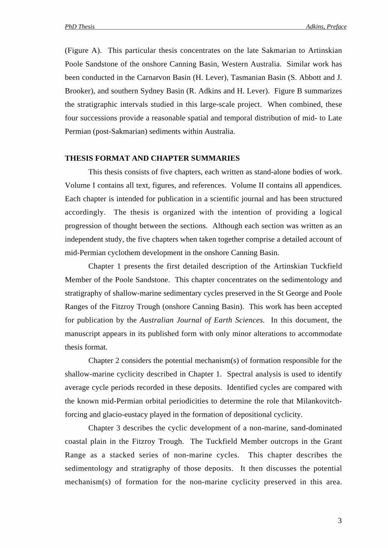
(Figure A). This particular thesis concentrates on the late Sakmarian to Artinskian
Poole Sandstone of the onshore Canning Basin, Western Australia. Similar work has
been conducted in the Carnarvon Basin (H. Lever), Tasmanian Basin (S. Abbott and J.
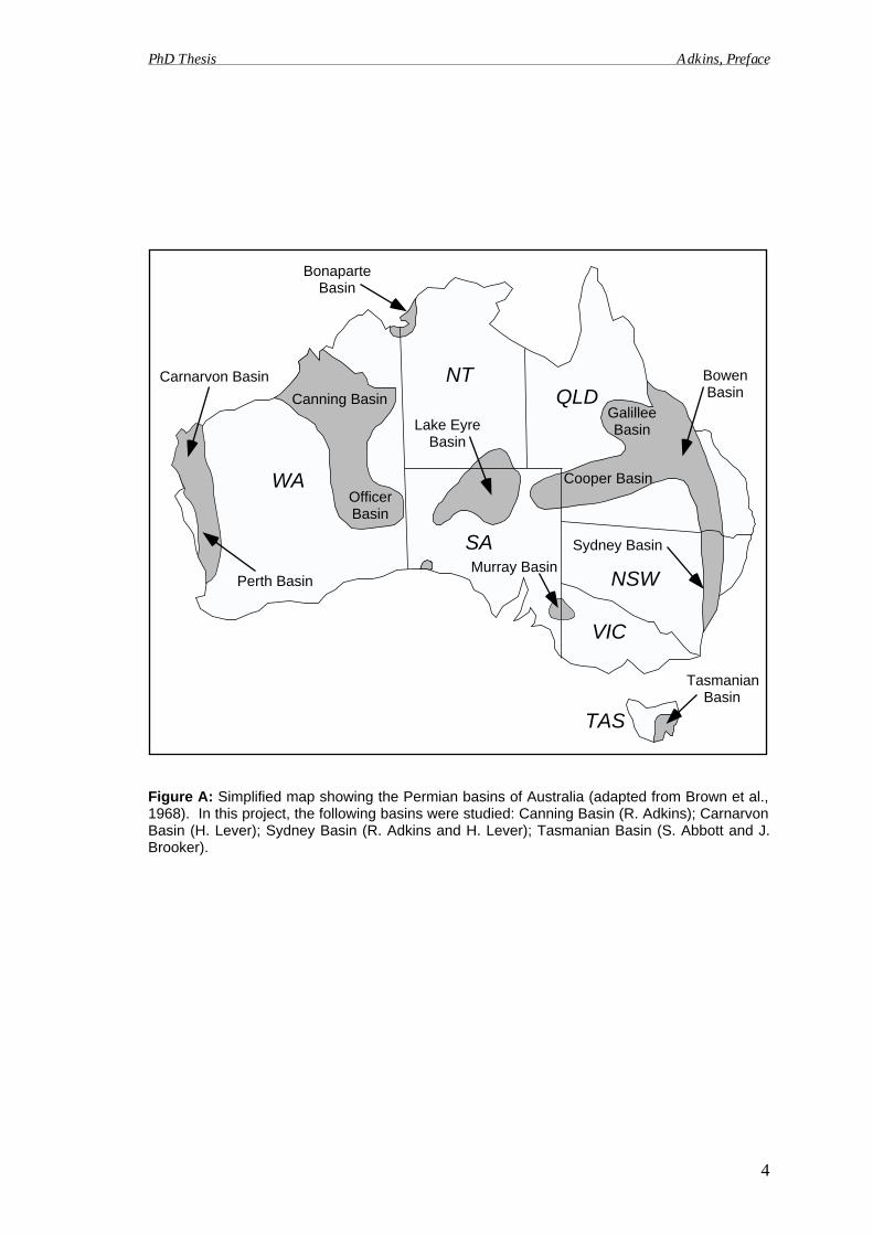
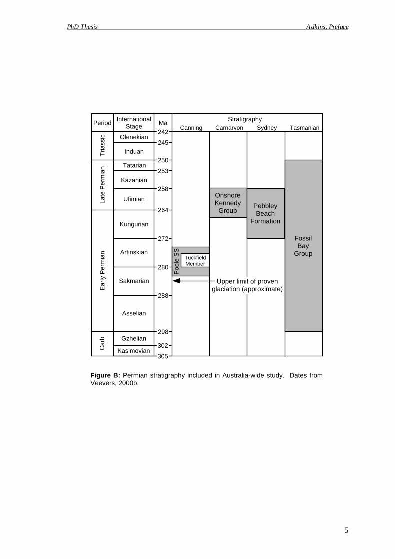
Brooker), and southern Sydney Basin (R. Adkins and H. Lever). Figure B summarizes
the stratigraphic intervals studied in this large-scale project. When combined, these
four successions provide a reasonable spatial and temporal distribution of mid- to Late
Permian (post-Sakmarian) sediments within Australia.
THESIS FORMAT AND CHAPTER SUMMARIES
This thesis consists of five chapters, each written as stand-alone bodies of work.
Volume I contains all text, figures, and references. Volume II contains all appendices.
Each chapter is intended for publication in a scientific journal and has been structured
accordingly. The thesis is organized with the intention of providing a logical
progression of thought between the sections. Although each section was written as an
independent study, the five chapters when taken together comprise a detailed account of
mid-Permian cyclothem development in the onshore Canning Basin.
Chapter 1 presents the first detailed description of the Artinskian Tuckfield
Member of the Poole Sandstone. This chapter concentrates on the sedimentology and
stratigraphy of shallow-marine sedimentary cycles preserved in the St George and Poole
Ranges of the Fitzroy Trough (onshore Canning Basin). This work has been accepted
for publication by the Australian Journal of Earth Sciences. In this document, the
manuscript appears in its published form with only minor alterations to accommodate
thesis format.
Chapter 2 considers the potential mechanism(s) of formation responsible for the
shallow-marine cyclicity described in Chapter 1. Spectral analysis is used to identify
average cycle periods recorded in these deposits. Identified cycles are compared with
the known mid-Permian orbital periodicities to determine the role that Milankovitch-
forcing and glacio-eustacy played in the formation of depositional cyclicity.
Chapter 3 describes the cyclic development of a non-marine, sand-dominated
coastal plain in the Fitzroy Trough. The Tuckfield Member outcrops in the Grant
Range as a stacked series of non-marine cycles. This chapter describes the
sedimentology and stratigraphy of those deposits. It then discusses the potential
mechanism(s) of formation for the non-marine cyclicity preserved in this area.
Carnarvon Basin
Perth Basin
Canning Basin
OfficerBasin
GalilleeBasin
Cooper Basin
Sydney Basin
Lake EyreBasin
TasmanianBasin
BowenBasin
NT
WA
SA
VIC
NSW
QLD
TAS
BonaparteBasin
Murray Basin
Figure A: Simplified map showing the Permian basins of Australia (adapted from Brown et al.,1968). In this project, the following basins were studied: Canning Basin (R. Adkins); CarnarvonBasin (H. Lever); Sydney Basin (R. Adkins and H. Lever); Tasmanian Basin (S. Abbott and J.Brooker).
PhD Thesis Adkins, Preface
4
MaPeriodInternational
StageStratigraphy
242
245
250
253
258
264
272
280
288
Tria
ssic
Late
Per
mia
nE
arly
Per
mia
n
Olenekian
Induan
Tatarian
Kazanian
Ufimian
Kungurian
Artinskian
Sakmarian
Asselian
Poo
le S
S
Canning Carnarvon TasmanianSydney
OnshoreKennedy
GroupPebbleyBeach
Formation
FossilBay
Group
302
305
Car
b Gzhelian
Kasimovian
298
Figure B: Permian stratigraphy included in Australia-wide study. Dates fromVeevers, 2000b.
Upper limit of provenglaciation (approximate)
PhD Thesis Adkins, Preface
5
TuckfieldMember
PhD Thesis Adkins, Preface
6
Chapter 4 considers the development of the Poole Sandstone (Nura Nura and
Tuckfield Members) on a regional scale. Thirty subsurface gamma-ray logs are used to
map the Poole Sandstone and trace cyclothem development throughout the northern
Fitzroy Trough and onto the adjacent Lennard Shelf (covering an area of approximately
15,000 km2).
For comparison, Chapter 5 addresses cyclothem development in the Pebbley
Beach Formation of the Shoalhaven Group (southern Sydney Basin, New South Wales).
If cycles identified in the Canning Basin are indeed glacio-eustatic in origin,
comparable cyclicity should be preserved in analogous environments worldwide. This
study utilizes the techniques developed in Western Australia to assess cyclicity recorded
in mid-Permian shallow-marine deposits in eastern Australia.
Chapter 1
Regressive systems tract cyclicity in shorezone deposits:the sedimentology and stratigraphy of the Early PermianTuckfield Member (Poole Sandstone), onshore Canning
Basin, Western Australia
PhD Thesis Adkins, Chapter 1
8
ABSTRACT
The Early Permian Tuckfield Member of the Poole Sandstone is exposed around
the periphery of the St George and Poole Ranges of the Fitzroy Trough (onshore
Canning Basin, Western Australia). It outcrops as a 50 to 100 m thick package of
vertically stacked, coarsening- and thickening-upward cycles. These cycles consist
upwards of siltstone, sandstone, and mud-pellet conglomerate, with minor amounts of
silty mudstone at the base of some cycles. At the outcrop scale, cycles range in
thickness from less than 5 m up to approximately 12 m and dictate the
geomorphological features of the area, with benches occurring at cycle tops. Primary
sedimentary structures, trace fossils, and the vertical succession of facies suggest that
each cycle records an episode of shorezone progradation. The Tuckfield Member in
the St George and Poole Ranges is here interpreted to consist predominantly of a
stacked series of regressive systems tract cycles.
Key Words: Canning Basin, cyclicity, Permian, Poole Sandstone, regressive systems
tract, Tuckfield Member
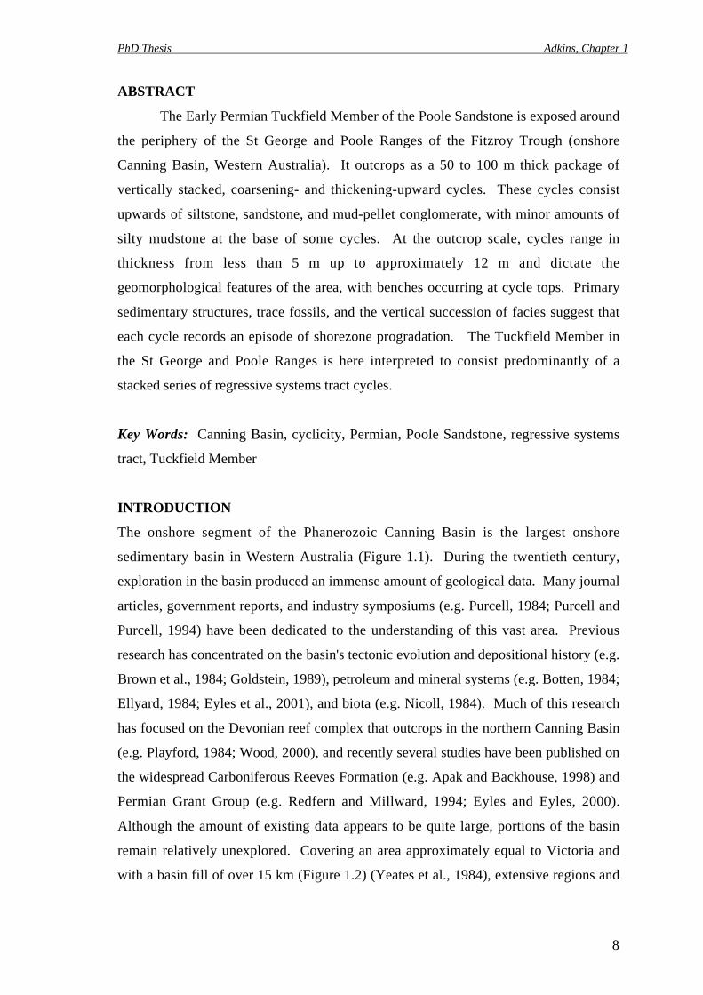
INTRODUCTION
The onshore segment of the Phanerozoic Canning Basin is the largest onshore
sedimentary basin in Western Australia (Figure 1.1). During the twentieth century,
exploration in the basin produced an immense amount of geological data. Many journal
articles, government reports, and industry symposiums (e.g. Purcell, 1984; Purcell and
Purcell, 1994) have been dedicated to the understanding of this vast area. Previous
research has concentrated on the basin's tectonic evolution and depositional history (e.g.
Brown et al., 1984; Goldstein, 1989), petroleum and mineral systems (e.g. Botten, 1984;
Ellyard, 1984; Eyles et al., 2001), and biota (e.g. Nicoll, 1984). Much of this research
has focused on the Devonian reef complex that outcrops in the northern Canning Basin
(e.g. Playford, 1984; Wood, 2000), and recently several studies have been published on
the widespread Carboniferous Reeves Formation (e.g. Apak and Backhouse, 1998) and
Permian Grant Group (e.g. Redfern and Millward, 1994; Eyles and Eyles, 2000).
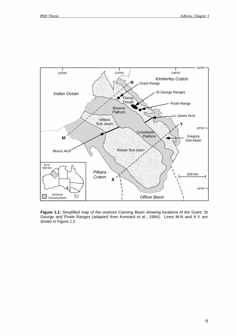
Although the amount of existing data appears to be quite large, portions of the basin
remain relatively unexplored. Covering an area approximately equal to Victoria and
with a basin fill of over 15 km (Figure 1.2) (Yeates et al., 1984), extensive regions and
200 km
500 km
Jones Arch
Munro Arch
BroomePlatform
M
YWillara
Sub -basin
Indian Ocean
Kimberley Craton
PilbaraCraton
Officer Basin
Poole Range
St George Ranges
Crosslands Platform
24º00´
20º00´
16º00´
128º00´124º00´120º00´
FitzroyTrough
Grant Range
Figure 1.1: Simplified map of the onshore Canning Basin showing locations of the Grant, StGeorge and Poole Ranges (adapted from Kennard et al., 1994). Lines M-N and X-Y areshown in Figure 1.2.
PhD Thesis Adkins, Chapter 1
GregorySub-basin
OnshoreCanning Basin
9
200 km
Triassic-Cretaceous
Late Carboniferous-Permian
Middle Devonian-Early Carboniferous
?Silurian-Early Devonian
Ordovician
Key
0
2
4
6
8
dept
h (k
m)
M N
YX
0
2
4
6
8
10
12
14
16
18
dept
h (k
m)
Willara Sub-basin Broome Platform Fitzroy Trough
GregorySub-basinKidson Sub-basin
SW NE
NESW
Figure 1.2: Schematic cross-section of the Canning Basin (adapted from Yeates et al., 1984).Location of section lines is shown in Figure 1.1.
PhD Thesis Adkins, Chapter 1
10
PhD Thesis Adkins, Chapter 1
11
many depositional units in the onshore Canning Basin have yet to be studied in any
detail.
The Early Permian Poole Sandstone (defined by Guppy et al., 1952, 1958) has
been considered as a potential petroleum reservoir (Jackson et al., 1994; Apak and
Carlsen, 1996), a source rock (Horstman, 1984; Kennard et al., 1994), and an important
aquifer (Yeates et al., 1984). Although it may thereby be economically important, the
Poole Sandstone remains poorly understood because few sedimentological and/or
stratigraphic analyses have been performed on this unit. In 1976, Crowe and Towner
published two brief reports on the Poole Sandstone: the first report introduced the
uppermost Christmas Creek Member (Crowe and Towner, 1976a), whereas the second
discussed the depositional environment of the lowermost Nura Nura Member (Crowe
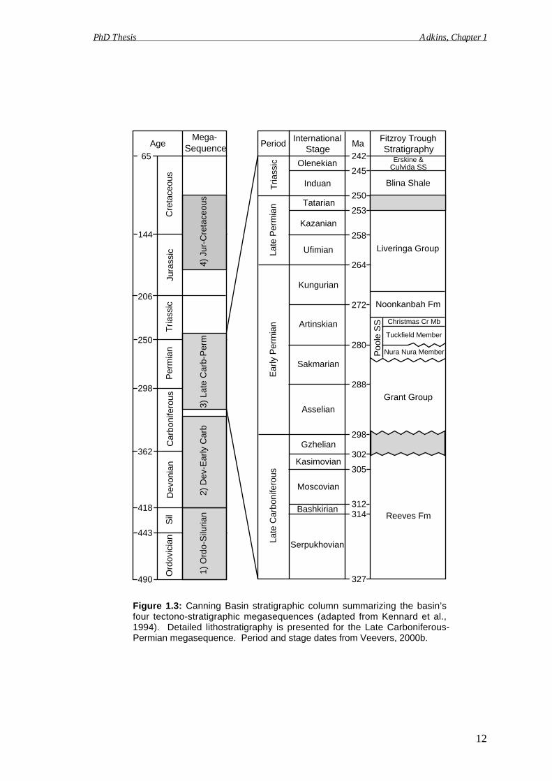
and Towner, 1976b) (Figure 1.3). Since 1976, the Geological Survey of Western
Australia and the Bureau of Mineral Resources (now Geoscience Australia) have
published general descriptions of the unit with geological maps (e.g. Crowe and
Towner, 1981; Gibson and Crowe, 1982) and in reports on Permo-Carboniferous
hydrocarbon prospectivity (Apak, 1996; Havord et al., 1997). Other than these few
government reports, only brief descriptions of the Poole Sandstone can be found in a
few large-scale overview papers (e.g. Yeates et al., 1984).
This article describes in detail the sedimentology and stratigraphy of the middle
Tuckfield Member of the Poole Sandstone (Figure 1.3). This work has practical
applications because it is the first in-depth study of the Tuckfield Member, thereby
providing a sedimentological and stratigraphic framework for this prospective unit.
Additionally, this paper lays the foundation for subsequent work addressing
Milankovitch-band cyclicity that is preserved in the Tuckfield Member.
METHODS
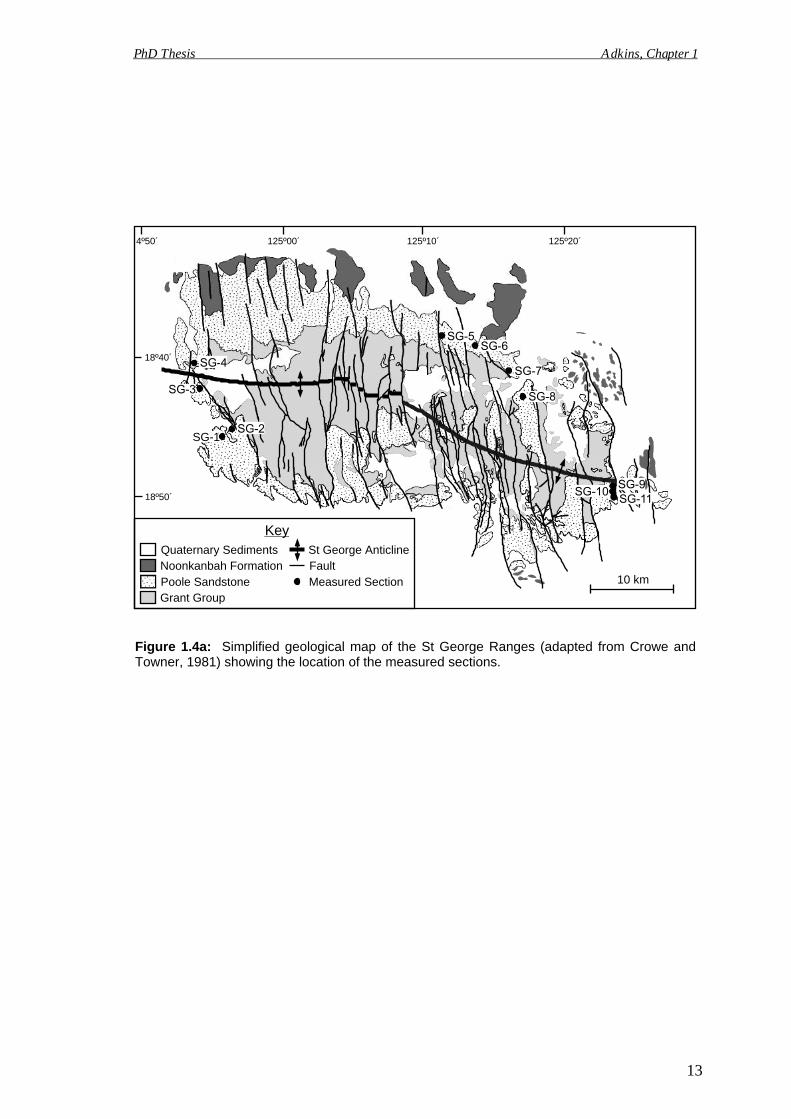
This research is based upon field investigations of the Tuckfield Member, where
it is exposed around the periphery of the St George and Poole Ranges of the Fitzroy
Trough (Figure 1.4; Appendix 1). Fifteen outcrop sections of the Tuckfield Member
were evaluated on a bed-by-bed basis for lithology, fossils, and sedimentary structures,
including bed thickness variations and vertical stacking of facies (Appendix 2).
Measured sections, ranging from 30 to 110 m thick, focus on the documentation of
repetitive, meter-scale cycles recorded within the succession. Based upon these
observations, an idealized cycle model has been developed for the Tuckfield Member.
MaPeriodInternational Fitzroy Trough
242
245
250
253
258
264
272
280
288
298
302
305
312314
Tria
ssic
Late
Per
mia
nE
arly
Per
mia
nLa
te C
arbo
nife
rous
Olenekian
Induan
Tatarian
Kazanian
Ufimian
Kungurian
Artinskian
Sakmarian
Asselian
Gzhelian
Kasimovian
Moscovian
Bashkirian
Serpukhovian
Blina Shale
Liveringa Group
Noonkanbah Fm
Poo
le S
S
Grant Group
Reeves Fm
Nura Nura Member
Tuckfield Member
Christmas Cr Mb
Cre
tace
ous
Jura
ssic
Tria
ssic
Per
mia
nC
arbo
nife
rous
Dev
onia
nS
ilO
rdov
icia
n443
362
298
250
206
144
65
1) O
rdo-
Silu
rian
2) D
ev-E
arly
Car
b3)
Lat
e C
arb-
Per
m4)
Jur
-Cre
tace
ous
AgeMega-
418
490 327
Figure 1.3: Canning Basin stratigraphic column summarizing the basin’sfour tectono-stratigraphic megasequences (adapted from Kennard et al.,1994). Detailed lithostratigraphy is presented for the Late Carboniferous-Permian megasequence. Period and stage dates from Veevers, 2000b.
PhD Thesis Adkins, Chapter 1
12
Erskine &Stratigraphy
Culvida SS
StageSequence
Noonkanbah FormationPoole Sandstone Measured Section
FaultSt George AnticlineQuaternary Sediments
Grant Group
Key
10 km
SG-1
18º40´
18º50´
125º00´ 125º10´ 125º20´4º50´
Figure 1.4a: Simplified geological map of the St George Ranges (adapted from Crowe andTowner, 1981) showing the location of the measured sections.
PhD Thesis Adkins, Chapter 1
13

10 km
Poole Sandstone Fault
Grant Group Measured Section
Poole AnticlineQuaternary Sediments
Key
125º50´
18º50´
Figure 1.4b: Simplified geological map of the Poole Range(adapted from Crowe and Towner, 1981) showing thelocation of the measured sections.
PhD Thesis Adkins, Chapter 1
14
PhD Thesis Adkins, Chapter 1
15
Gamma-ray measurements were collected from each outcrop at a 0.5 m spacing
and plotted against the corresponding lithological log (Appendices 2 and 3). Gamma-
ray emissions are related to the content of radiogenic isotopes of potassium, uranium,
and thorium. These elements (particularly potassium) are common in clay minerals
(Cant, 1992) and hence, the gamma-ray log from each measured section should reflect
the amount of clay present and quantitatively detect changes in lithology.
To better understand the nature of the Tuckfield Member, one typical cycle was
analyzed in detail. Ten hand-sized samples were collected from a 3.5 m section of
outcrop (one cycle) located on the eastern side of the St George Ranges. Thin-sections
were prepared for each sample and analyzed for cycle trends. Petrographic data,
including mineralogy, grainsize, roundness, sorting, and porosity, were recorded from
each thin-section. Porosities were calculated using the following method. Rock chips
were impregnated with dyed epoxy before being made into thin-sections. Digital
photographs were taken of the thin-sections and set to a scale of 256 greys (Appendix
4). In the grey-scale photographs, epoxy-filled pore spaces are easily differentiated
from the samples' mineralogy. For each thin-section, the computer program NIH was
used to create a density slice corresponding to pore space. The area of each density
slice was then calculated and used as a proxy for the rock's porosity (Appendix 5). XRF
and quantitative XRD data (Appendix 6) were also collected from each hand-sample to
better constrain compositional and mineralogical trends in the cycle.
REGIONAL SETTING AND DEPOSITIONAL HISTORY
The onshore Canning Basin is a broad, intracratonic rift basin located between
the Proterozoic Kimberley Craton to the northeast and the Archean Pilbara Craton to the
southwest (Figure 1.1) (Purcell, 1984). Cretaceous sediments in the basin extend
southward, connecting the Canning Basin to the Phanerozoic Officer Basin (Yeates et
al., 1984).
Although the onshore Canning Basin is now quite stable, it had a complex
tectonic evolution that lasted from the Early Ordovician to the Tertiary. At ca 500 Ma,
thrust-related shearing in basement rock to the north (Shaw et al., 1992a) resulted in
extension, rapid subsidence, and the formation of the basin. Successive episodes of
crustal stretching followed by tectonic quiescence resulted in the deposition of four
tectono-stratigraphic megasequences: (i) Ordovician-Silurian; (ii) Devonian-Early
PhD Thesis Adkins, Chapter 1
16
Carboniferous; (iii) Late Carboniferous-Permian; and (iv) Jurassic-Cretaceous (Kennard
et al., 1994) (Figure 1.3).
This paper focuses on deposits of the Late Carboniferous-Permian
megasequence (Figure 1.3). The deposition of this megasequence was initiated by
compression and inversion of pre-existing Devonian faults (Meda Transpressional
Movement) during the mid-Carboniferous. This movement probably coincided with the
peak of the Alice Springs Orogeny, when Laurasia and Gondwana collided, subjecting
much of western and central Australia to compression and uplift (Shaw et al., 1992b).
In the Canning Basin, this time is marked by the deposition of syntectonic fluvial,
glaciofluvial, and glaciomarine deposits (Kennard et al., 1994; Redfern and Millward,
1994) of the Reeves Formation (formerly the Lower Grant Group: Apak and
Backhouse, 1998) (Figure 1.3). By the earliest Permian, renewed extension and rapid
subsidence (Point Moody Extensional Movement) corresponded with continued glacial
conditions (Kennard et al., 1994) and deposition of the Grant Group (formerly the
Upper Grant Group: Apak and Backhouse, 1998). Following the Point Moody
Extensional Movement, the basin entered an extended period of tectonic quiescence that
was interrupted by short pulses of regional tectonism. This period was also marked by
the widespread deposition of a transgressive, shallow-marine sand sheet (Poole
Sandstone) that coincided with the termination of glacial conditions throughout the
basin. From the mid-Permian to the Early Triassic, two successive third-order
transgressive-regressive cycles (Poole-Noonkanbah-Liveringa and Blina-Erskine),
consisting of marine shale and siltstone overlain by shallow shelf and fluvial sandstone,
were deposited in the Canning Basin (Kennard et al., 1994).
Today, regionally-extensive, northwest-trending extensional faults define the
predominant structure of the basin (Kennard et al., 1994). Two major northwest-
trending depositional troughs are separated by an uplifted mid-basin arch (Figures 1.1
and 1.2). This arch dips gently to the southeast and is capped by a thin succession (1-2
km) of predominantly Ordovician, Devonian and Permian rocks (Bentley, 1984). The
elongated northern trough contains up to 18 km of predominantly Devonian and
younger sediments. It is further divided by a basement high (the Jones Arch) into the
asymmetrical Fitzroy Trough to the northwest and the Gregory Sub-basin to the
southeast. The southern trough contains a 4 to 5 km thick succession of Ordovician to
Silurian rocks with a thin cap (approximately 1-2 km) of Devonian and younger
sediments (Kennard et al., 1994). The southern trough is divided by a basement high
PhD Thesis Adkins, Chapter 1
17
(the Munro Arch) into the Willara Sub-basin to the northwest and the broad Kidson
Sub-basin to the southeast.
THE TUCKFIELD MEMBER OF THE POOLE SANDSTONE
The Tuckfield Member is one of three distinct depositional units that together
comprise the Poole Sandstone. The Poole Sandstone is a laterally extensive package of
shallow-marine and non-marine sediments. It consists of the lower Nura Nura Member,
the middle Tuckfield Member, and the upper Christmas Creek Member (Figure 1.3).
Today, the Poole Sandstone is predominantly encountered in the sub-surface. However,
dextral wrench faulting in the Late Triassic to Early Jurassic (Fitzroy Transpressional
Movement) uplifted and exposed thick outcrop sections of the Poole Sandstone in a few
locations throughout the basin (Kennard et al., 1994).
The best exposures of the Tuckfield Member are found in the Grant, St George,
and Poole Ranges of the Fitzroy Trough (Figure 1.1; Appendix 1). This study
concentrates on outcrops around the periphery of the St George and Poole Ranges. In
these areas, the Tuckfield Member conformably to disconformably overlies the Nura
Nura Member and conformably underlies the Christmas Creek Member. In the Fitzroy
Trough, no age-diagnostic fossils occur in the Tuckfield Member. However,
palynomorphs from elsewhere in the basin indicate an early to late Artinskian age for
this unit (Figure 1.3) (Yeates et al., 1975).
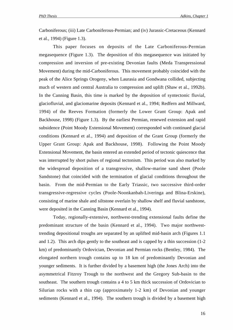
In the St George and Poole Ranges, the Tuckfield Member outcrops as a series
of small (up to approximately 150 m high), rounded hills (Figure 1.5). Each hill
comprises multiple, vertically stacked, flat-lying benches that can be traced laterally for
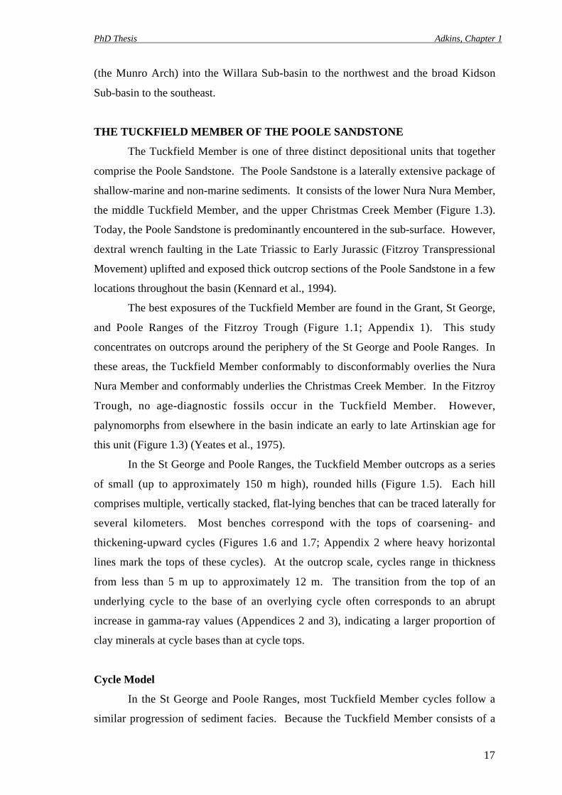
several kilometers. Most benches correspond with the tops of coarsening- and
thickening-upward cycles (Figures 1.6 and 1.7; Appendix 2 where heavy horizontal
lines mark the tops of these cycles). At the outcrop scale, cycles range in thickness
from less than 5 m up to approximately 12 m. The transition from the top of an
underlying cycle to the base of an overlying cycle often corresponds to an abrupt
increase in gamma-ray values (Appendices 2 and 3), indicating a larger proportion of
clay minerals at cycle bases than at cycle tops.
Cycle Model
In the St George and Poole Ranges, most Tuckfield Member cycles follow a
similar progression of sediment facies. Because the Tuckfield Member consists of a
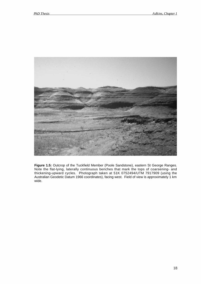
Figure 1.5: Outcrop of the Tuckfield Member (Poole Sandstone), eastern St George Ranges.Note the flat-lying, laterally continuous benches that mark the tops of coarsening- andthickening-upward cycles. Photograph taken at 51K 0752494/UTM 7917909 (using theAustralian Geodetic Datum 1966 coordinates), facing west. Field of view is approximately 1 kmwide.
PhD Thesis Adkins, Chapter 1
18
30
90 310
40
10
Nur
aT
uckf
ield
X-m
as
200gamma-ray claysand
sedimentarystructures c z vf fl fu m c
?
?
?
0 mvc
20
Poole Range Outcrop (Location P-2)
Cre
ekN
ura
Figure 1.6a: Lithology log with associated gamma-ray data from the PooleRange. The base of the measured section is located at 51K 0795598/UTM7913141 (using the Australian Geodetic Datum 1966 coordinates). Heavyhorizontal lines mark the tops of coarsening- and thickening-upward cycles.These lines generally correspond to the benches shown in Figure 1.5.Grainsize increments from left to right on x-axis are as follows: c (clay/mud);z (silt); vf (very fine sand); fl (lower half of fine sand); fu (upper half of finesand); m (medium sand); c (coarse sand); vc (very coarse sand). Fine sandwas divided into lower and upper halves to better depict variations ingrainsize. Member names are given in the right-hand column. See Figure1.6b for key.
PhD Thesis Adkins, Chapter 1
19
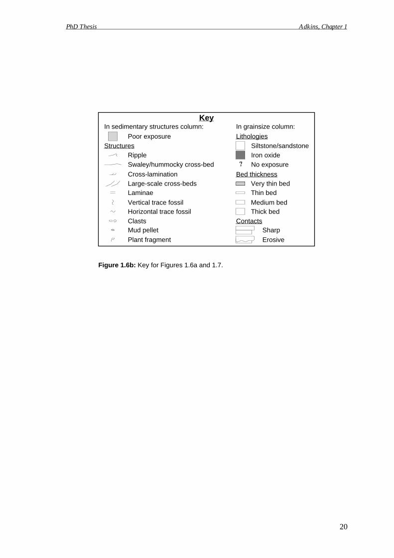
Ripple
Swaley/hummocky cross-bed
Iron oxide
Cross-lamination
No exposure
Thin bedLaminaeVery thin bed
Horizontal trace fossil
Contacts
Vertical trace fossilThick bed
Plant fragment
Clasts
Erosive
SharpMud pellet
Large-scale cross-bedsBed thickness
Poor exposure Lithologies
Siltstone/sandstoneStructures
In grainsize column:In sedimentary structures column:
Medium bed
Key
Figure 1.6b: Key for Figures 1.6a and 1.7.
PhD Thesis Adkins, Chapter 1
20
30
10
20
40
60
?
50
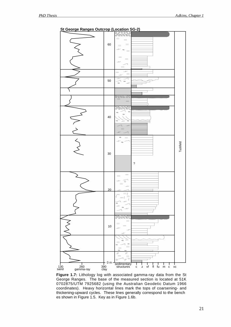
sedimentarystructures c z vf fl fu m c vc130 390260
gamma-ray claysand
0 m
Tuck
field
St George Ranges Outcrop (Location SG-2)
Figure 1.7: Lithology log with associated gamma-ray data from the StGeorge Ranges. The base of the measured section is located at 51K0702875/UTM 7925682 (using the Australian Geodetic Datum 1966coordinates). Heavy horizontal lines mark the tops of coarsening- andthickening-upward cycles. These lines generally correspond to the bench-es shown in Figure 1.5. Key as in Figure 1.6b.
PhD Thesis Adkins, Chapter 1
21
PhD Thesis Adkins, Chapter 1
22
repetitive, vertically stacked series of cycles, a generalized cycle model can be used to
describe the basic sedimentology of the Tuckfield Member in this area (Figure 1.8).
A scree-covered, gentle slope often occurs at the base of cycles. This area of
poor exposure usually grades upward from silty mudstone to very thin-bedded, rippled
siltstone with asymmetrical cross-lamination (Figure 1.9a). These deposits gradually
coarsen and thicken upward to medium-bedded, fine-grained sandstone. Within this
coarsening- and thickening-upward package, ripple cross-laminated beds are gradually
replaced by beds with flat-lying, internal laminae. Symmetrical ripple marks occur
throughout the cycle, but are more prevalent near the base, whereas non-rippled beds
are more prevalent near the top of the cycle. Ripple marks record a variety of bi-
directional currents with a dominant paleo-flow to the northwest/southeast (Appendix
7). Beds tend to be laterally continuous with non-erosive to slightly erosive bases.
Detrital muscovite flakes often occur on bedding planes. Thin beds of iron oxide and
surficial ferruginization are common throughout this package. Abundant horizontal
trace fossils, typical of a Cruziana ichnofacies, often occur on bedding planes and are
preferentially preserved in the ferruginous zones (Figure 1.9b).
Overlying this gradually coarsening- and thickening-upward succession is
medium- to thick-bedded, medium-grained sandstone. These thicker sands can be: (i)
massive; (ii) have large-scale, trough- to planar-cross beds; or (iii) consist of a series of
extremely faint, thin to medium beds with planar laminations. These coarser sand
bodies usually have erosive bases and often contain abundant vertical burrows, typical
of a Skolithos ichnofacies (Figure 1.9c). Rare root beds are also present.
Iron-rich, silty mud-pellet and plant-fragment conglomerates occasionally cap
these cycles (Figure 1.9d). The silty mud pellets tend to be elongated and bedding-
parallel, with a muddy center and a thick (up to 1 cm) iron-oxide outer shell. The
conglomerates have an iron-rich sandy matrix. They occur in the western part of the
area. They range in thickness from a few centimeters up to approximately 1 m. The
thinner beds typically occur in the central part of the St George Ranges, whereas the
thicker beds typically occur in the western part of these ranges.
Detailed Cycle Analyses
One cycle was studied in detail to gain a better understanding of cycle
development in the Tuckfield Member. A particular cycle was chosen based upon its
representative nature and total thickness. Ten hand-sized samples were analyzed for
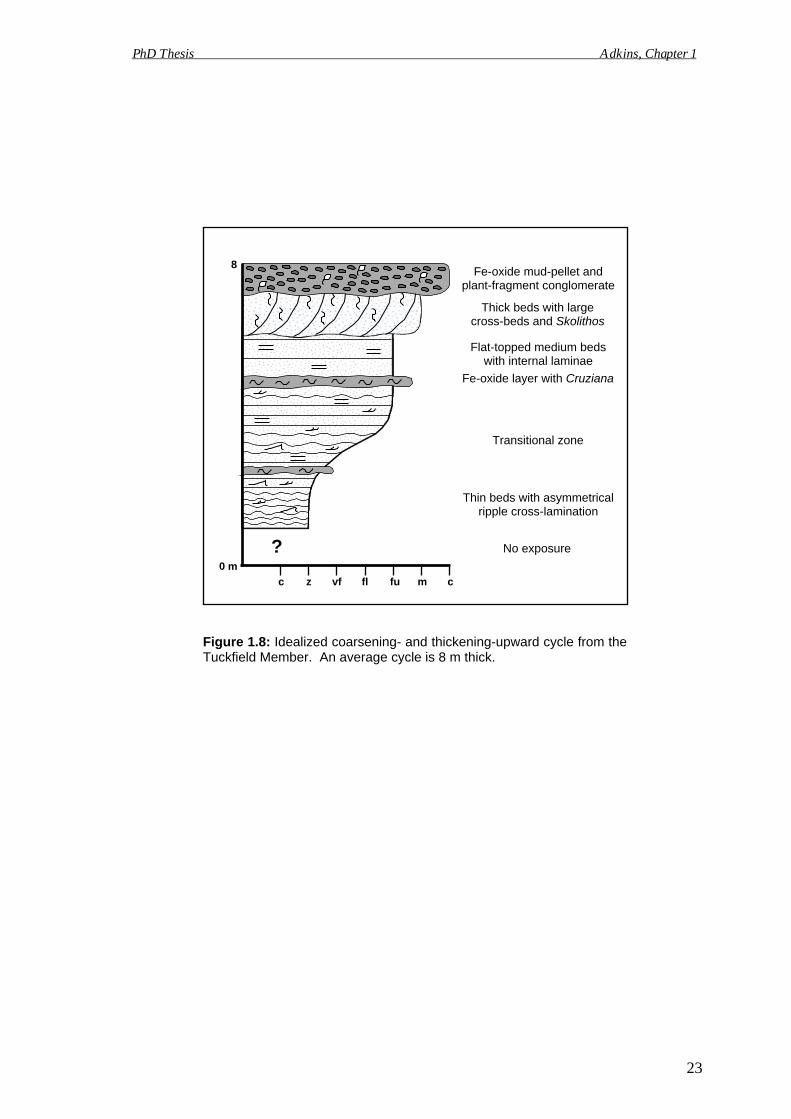
c z vf fl fu m c
0 m
8
? No exposure
Thin beds with asymmetricalripple cross-lamination
Fe-oxide layer with Cruziana
Flat-topped medium bedswith internal laminae
Transitional zone
Thick beds with largecross-beds and Skolithos
Fe-oxide mud-pellet andplant-fragment conglomerate
Figure 1.8: Idealized coarsening- and thickening-upward cycle from theTuckfield Member. An average cycle is 8 m thick.
PhD Thesis Adkins, Chapter 1
23
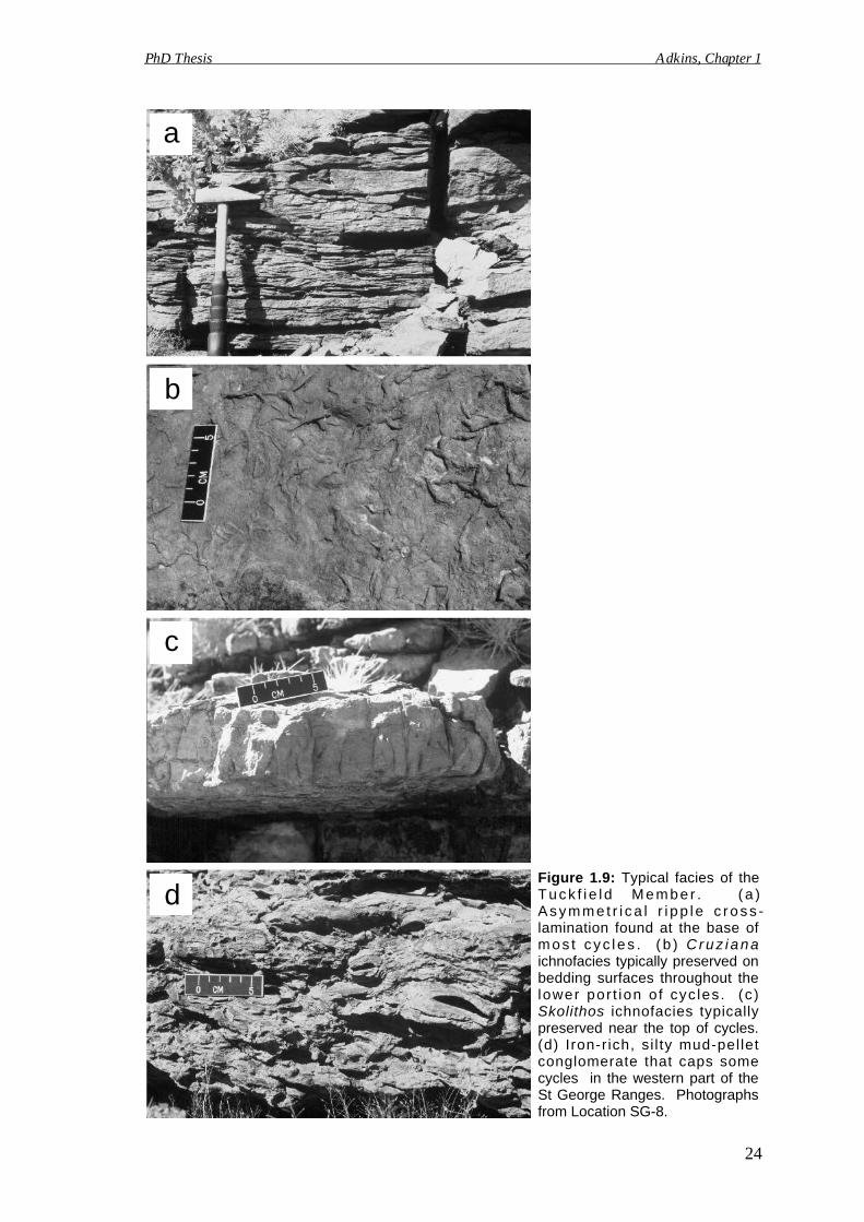
Figure 1.9: Typical facies of theT u c k f i e l d M e m b e r . ( a )A s y m m e t r i c a l r i p p l e c r o s s -lamination found at the base ofm o s t c y c l e s . ( b ) C r u z i a n aichnofacies typically preserved onbedding surfaces throughout thelower por t ion o f cyc les . (c )Skolithos ichnofacies typicallypreserved near the top of cycles.(d) Iron-rich, si l ty mud-pelletconglomerate that caps somecycles in the western part of theSt George Ranges. Photographsfrom Location SG-8.
a
b
c
d
PhD Thesis Adkins, Chapter 1
24
PhD Thesis Adkins, Chapter 1
25
petrographic (grainsize, roundness, sorting, and porosity) and geochemical (XRF and
quantitative XRD) information. The base of the cycle could not be analyzed because of
poor outcrop exposure.
PETROGRAPHY
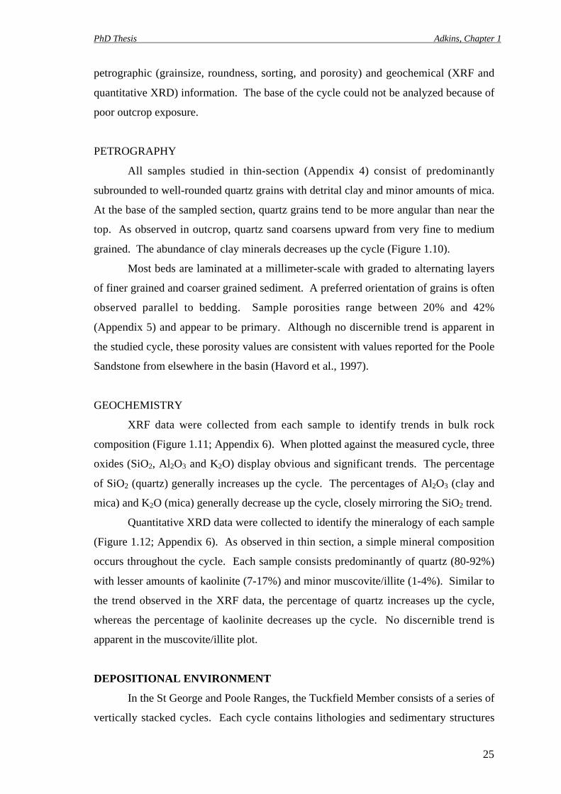
All samples studied in thin-section (Appendix 4) consist of predominantly
subrounded to well-rounded quartz grains with detrital clay and minor amounts of mica.
At the base of the sampled section, quartz grains tend to be more angular than near the
top. As observed in outcrop, quartz sand coarsens upward from very fine to medium
grained. The abundance of clay minerals decreases up the cycle (Figure 1.10).
Most beds are laminated at a millimeter-scale with graded to alternating layers
of finer grained and coarser grained sediment. A preferred orientation of grains is often
observed parallel to bedding. Sample porosities range between 20% and 42%
(Appendix 5) and appear to be primary. Although no discernible trend is apparent in
the studied cycle, these porosity values are consistent with values reported for the Poole
Sandstone from elsewhere in the basin (Havord et al., 1997).
GEOCHEMISTRY
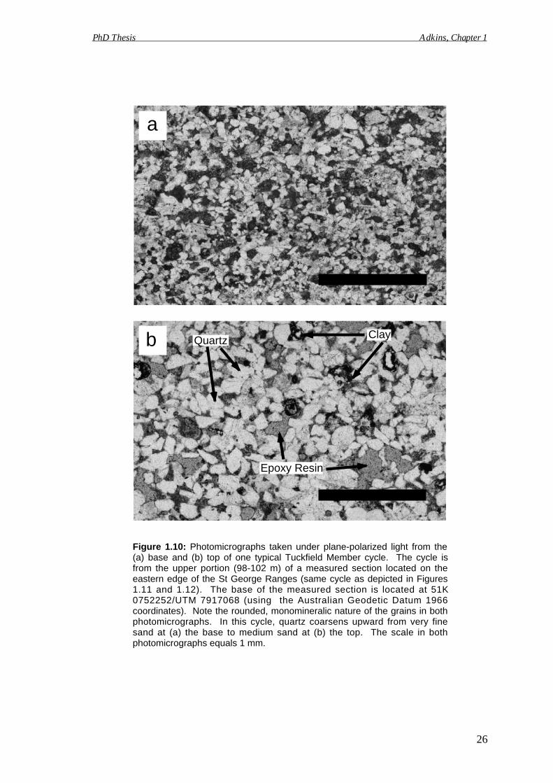
XRF data were collected from each sample to identify trends in bulk rock
composition (Figure 1.11; Appendix 6). When plotted against the measured cycle, three
oxides (SiO2, Al2O3 and K2O) display obvious and significant trends. The percentage
of SiO2 (quartz) generally increases up the cycle. The percentages of Al2O3 (clay and
mica) and K2O (mica) generally decrease up the cycle, closely mirroring the SiO2 trend.
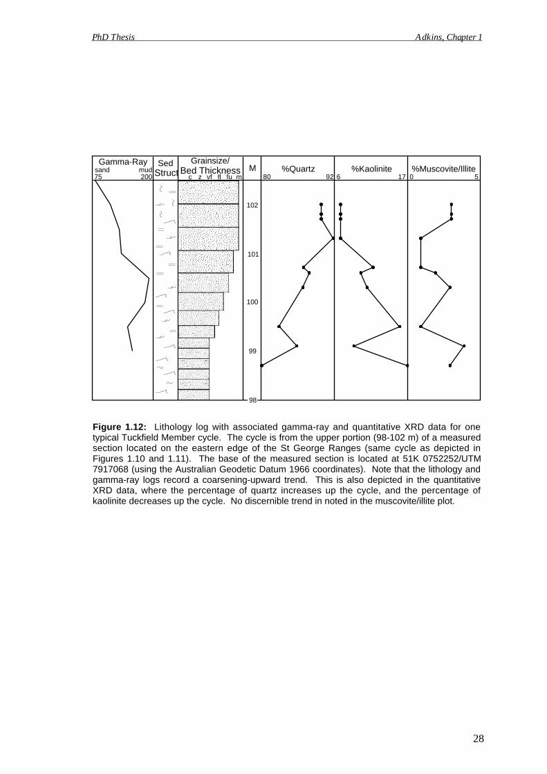
Quantitative XRD data were collected to identify the mineralogy of each sample
(Figure 1.12; Appendix 6). As observed in thin section, a simple mineral composition
occurs throughout the cycle. Each sample consists predominantly of quartz (80-92%)
with lesser amounts of kaolinite (7-17%) and minor muscovite/illite (1-4%). Similar to
the trend observed in the XRF data, the percentage of quartz increases up the cycle,
whereas the percentage of kaolinite decreases up the cycle. No discernible trend is
apparent in the muscovite/illite plot.
DEPOSITIONAL ENVIRONMENT
In the St George and Poole Ranges, the Tuckfield Member consists of a series of
vertically stacked cycles. Each cycle contains lithologies and sedimentary structures
a
b Clay
Epoxy Resin
Figure 1.10: Photomicrographs taken under plane-polarized light from the(a) base and (b) top of one typical Tuckfield Member cycle. The cycle isfrom the upper portion (98-102 m) of a measured section located on theeastern edge of the St George Ranges (same cycle as depicted in Figures1.11 and 1.12). The base of the measured section is located at 51K0752252/UTM 7917068 (using the Australian Geodetic Datum 1966coordinates). Note the rounded, monomineralic nature of the grains in bothphotomicrographs. In this cycle, quartz coarsens upward from very finesand at (a) the base to medium sand at (b) the top. The scale in bothphotomicrographs equals 1 mm.
PhD Thesis Adkins, Chapter 1
26
Quartz
99
100
101
102
98
%SiO287 95 3 8
%Al2O30.05 0.30
%K2Oc z vf fl fu m
MGrainsize/SedGamma-Ray
75 200sand mud
Figure 1.11: Lithology log with associated gamma-ray and XRF data for one typical TuckfieldMember cycle. The cycle is from the upper portion (98-102 m) of a measured section locatedon the eastern edge of the St George Ranges (same cycle as depicted in Figures 1.10 and1.12). The base of the measured section is located at 51K 0752252/UTM 7917068 (using theAustralian Geodetic Datum 1966 coordinates). Note that the lithology and gamma-ray logsrecord a coarsening-upward trend. This is also depicted in the XRF data, where thepercentage of SiO 2 (quartz) increases up the cycle, and the percentages of Al 2O3 (clay and
mica) and K2O (mica) decrease up the cycle.
Bed ThicknessStruct
PhD Thesis Adkins, Chapter 1
27
99
100
101
102
98
c z vf fl fu mM
Grainsize/SedGamma-Ray
75 200sand mud %Quartz
80 92%Kaolinite
6 17 0 5%Muscovite/Illite
Figure 1.12: Lithology log with associated gamma-ray and quantitative XRD data for onetypical Tuckfield Member cycle. The cycle is from the upper portion (98-102 m) of a measuredsection located on the eastern edge of the St George Ranges (same cycle as depicted inFigures 1.10 and 1.11). The base of the measured section is located at 51K 0752252/UTM7917068 (using the Australian Geodetic Datum 1966 coordinates). Note that the lithology andgamma-ray logs record a coarsening-upward trend. This is also depicted in the quantitativeXRD data, where the percentage of quartz increases up the cycle, and the percentage ofkaolinite decreases up the cycle. No discernible trend in noted in the muscovite/illite plot.
PhD Thesis Adkins, Chapter 1
Struct Bed Thickness
28
PhD Thesis Adkins, Chapter 1
29
that are indicative of a prograding sandy shorezone (as defined by Galloway and
Hobday, 1996) (Figure 1.13). All data presented herein (field observations, gamma-ray
logs, petrography, and geochemical analyses) are consistent with each cycle coarsening
and shallowing upwards. Sedimentary structures near the base of most cycles
(asymmetrical ripple cross-lamination, Cruziana ichnofacies) are indicative of
deposition in a high-energy, lower to middle shoreface environment. Sedimentary
structures near the top of most cycles (flat-lying beds, low-angle planar laminae,
Skolithos ichnofacies) are indicative of deposition in a high-energy, upper shoreface to
foreshore environment. Erosive beds throughout the Tuckfield Member may record
storm events or mark the location of rip or tidal channels.
The mud-pellet conglomerates that cap many Tuckfield cycles were previously
noted by Yeates et al. (1984). In the same paper, the authors suggest that similar iron-
rich beds in the Liveringa Group (Lightjack Formation: Figure 1.3) may have
precipitated where saltwater and freshwater mixed. I suggest that the Tuckfield
conglomerates probably formed in a supratidal mud-flat environment. This would
account for the presence of the finer grained sediment that is otherwise largely absent in
the Tuckfield Member. By the Artinskian, the climate of northern Western Australia
was starting to become progressively warmer and drier (Scotese et al., 1999). In such
climates, supratidal deposits can be oxidized and deformed by desiccation. Therefore,
supratidal environments in the Canning Basin would have been ideal for the formation
of oxidized, iron-coated mud pellets. Subsequent drowning, associated with storm
events or relative sea-level change, could have introduced the coarser grained sediment
that now forms the matrix of the Tuckfield Member conglomerates.
SEQUENCE STRATIGRAPHIC FRAMEWORK
The discipline of sequence stratigraphy began in the mid-1970’s with the work
of Peter Vail and his collegues at Exxon petroleum company (in Payton, 1977). Using
seismic data, the Vail group recognized a series of unconformity-bounded sequences in
the stratigraphic record. This work introduced the now popular concept of systems
tracts and lead to the development of the sequence stratigraphic model.
Contemporaneously, the Vail group asserted that, through sequence analysis, an
accurate chart of relative sea-level change could be constructed (Vail et al., 1977).
Exxon’s global model recognized several orders of sea-level fluctuation, ranging from a
few million years (3rd order cycles) to tens of millions of years (2nd order cycles) to
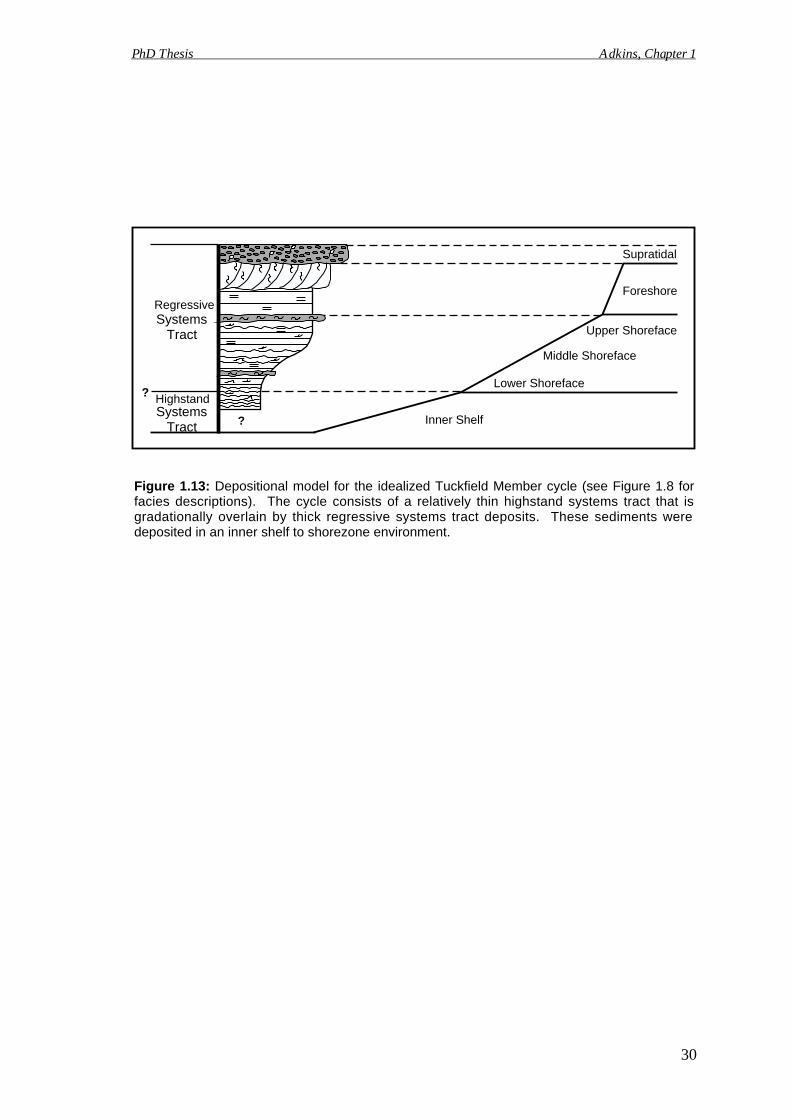
Foreshore
Upper Shoreface
Middle Shoreface
Lower Shoreface
Inner Shelf
Supratidal
?
?
Regressive
Highstand
Figure 1.13: Depositional model for the idealized Tuckfield Member cycle (see Figure 1.8 forfacies descriptions). The cycle consists of a relatively thin highstand systems tract that isgradationally overlain by thick regressive systems tract deposits. These sediments weredeposited in an inner shelf to shorezone environment.
PhD Thesis Adkins, Chapter 1
30
SystemsTract
SystemsTract
PhD Thesis Adkins, Chapter 1
greater than one hundred million years (1st order cycles). Although higher frequency
Milankovitch-scale cycles (20,000 to 100,000 years) were not included in Vail’s
original sea-level curve, they have been well documented elsewhere in the literature
(e.g. Shackleton and Opdyke, 1976; Abbott and Carter, 1994; Tiedemann et al., 1994;
Zachos et al., 1997).
In accordance with Vail’s sea-level curve, the Exxon sequence stratigraphic
model describes the idealized architecture of sediments deposited during a single sea-
level cycle. These deposits are divided into three main, geometrically separate
stratigraphic bodies, termed systems tracts (e.g. Vail et al., 1991). The lowstand
systems tract consists of sediments deposited at and around a sea-level lowstand. The
transgressive systems tract is deposited during the rising part of the sea-level cycle,
whereas the highstand systems tract is deposited mainly during and shortly after a sea-
level cycle peak.
In the original Exxon model, sedimentation does not occur on the shelf during
the falling portion of the sea-level cycle since this is typically a time of erosion.
However, subsequent studies (e.g. Hunt and Tucker, 1992; Posametier et al., 1992;
Naish and kamp, 1997) have demonstrated that deposition may occur on the shelf if the
correct balance of relative sea-level fall and rate of sediment supply is met. In such
cases, the term forced regressive systems tract applies when sediments are bounded
below by a regressive surface of erosion (Hunt and Tucker, 1992; Plint, 1988). The
term regressive systems tract applies when regressive deposits shoal gradationally
upwards from shelf into shoreface facies (Naish and Kamp, 1997).
Naish and Kamp (1997) first introduced and defined the regressive systems tract
based upon Plio-Pleistocene cycles from the Rangitikei River Valley (Wanganui Basin,
North Island, New Zealand). The deposits described by them consist of gradationally
based, strongly progradational, shoreline sediments that accumulated during falling sea-
level.
Similar in nature to the Rangitikei cyclothems, a typical Tuckfield Member
cycle consists of gradationally based, strongly progradational, shoreline sediments that
probably accumulated during falling sea-level. Therefore, the Tuckfield Member can
be interpreted as almost entirely regressive systems tract deposits (Figure 1.13). The
poorly exposed silty mudstone at the base of some cycles may represent inner shelf
sediments that belong to the highstand systems tract. However, these finer-grained,
31
PhD Thesis Adkins, Chapter 1
poorly exposed deposits are typically thin and grade upward into the thicker shoreface
and foreshore sediments that are herein ascribed to the regressive systems tract.
CONCLUSIONS
This is the first detailed investigation into the sedimentology and stratigraphy of
the Early Permian Tuckfield Member of the Poole Sandstone. In the St George and
Poole Ranges, at least 12 vertically stacked, coarsening- and thickening-upward
Tuckfield Member cycles have been identified in outcrop. These cycles range in
thickness from less than 5 m up to approximately 12 m. Each cycle contains lithologies
and sedimentary structures that are indicative of a prograding sandy shorezone. Based
on the data presented here, the Tuckfield Member is interpreted to consist
predominantly of a vertically stacked series of regressive systems tract cycles.
32
Chapter 2
High-frequency sedimentary cycles from the onshoreCanning Basin, Western Australia: an evaluation of the
effects of mid-Permian orbital forcing
PhD Thesis Adkins, Chapter 2
34
ABSTRACT
The Artinskian Tuckfield Member of the Poole Sandstone outcrops around the
periphery of the St George and Poole Ranges of the Fitzroy Trough (onshore Canning
Basin, Western Australia). In this area, the Tuckfield Member consists of a series of
laterally extensive, coarsening- and thickening-upward cycles that were deposited
predominantly in a shorezone environment. In outcrop, these cycles are typically 5 to
12 m thick. Gamma-ray and grainsize data, collected from 15 outcrops located
throughout the study area, were analyzed to better define cyclicity. Spectral analysis
identified several orders of meter- to decameter-scale cycles recorded in the Tuckfield
Member. The average periodicities of the identified cycles occur in the ratio of
~36:10:4:2 m. This ratio correlates strongly with the known mid-Permian orbital
periodicities of elongated eccentricity, eccentricity, obliquity, and precession
(~410:100:40:20 thousand years). This favorable comparison indicates that
Milankovitch-forcing and glacio-eustacy probably controlled the formation of
depositional cyclicity in the Tuckfield Member. The 5 to 12 m cycle, predominant in
outcrop, suggests that eccentricity and possibly obliquity were the main influences on
global sea-level fluctuation during this time. If these interpretation are correct, Permo-
Carboniferous glaciation persisted into at least the Artinskian stage of the Early
Permian.
Key Words: Canning Basin, glacio-eustacy, Late Paleozoic glaciation, Milankovitch
cyclicity, Permian, Poole Sandstone, Tuckfield Member
INTRODUCTION
Permo-Carboniferous sedimentary rocks record the longest known period of
Phanerozoic glaciation. During this time continental ice-sheets flourished on
Gondwana as it slowly drifted across the south pole (Crowell, 1975; Crowell, 1995). A
direct record of this glaciation can be found on all present-day Gondwanan continents
(Africa, Antarctica, Asia, Australia, and South America) as ice-affected landscapes and
glacial deposits (e.g. Crowell, 1978; Hambrey and Harland, 1981; Visser, 1989;
Gonzalez-Bonorino and Eyles, 1995). This record indicates that glaciation extended
into the Sakmarian stage of the Early Permian. Although the Sakmarian probably
marks the end of widespread Gondwanan glaciation (Scotese et al., 1999), there is
debatable evidence that ice-sheets may have remained on parts of Gondwana up to at
PhD Thesis Adkins, Chapter 2
35
least the Triassic boundary (Veevers et al., 1994a; Veevers, 2000a). However, due to
the ambiguous nature of this data, much uncertainty still exists concerning the exact
timing of Permo-Carboniferous deglaciation.
Fortunately, the direct evidence that is restricted to ice-proximal environments
(striated pavements, tillites, and outwash deposits) is not necessary to infer the presence
of massive continental ice-sheets and polar ice-caps. Periodic to quasi-periodic
oscillations in Earth's orbital parameters affect the distribution and amount of incident
solar energy reaching Earth's surface (Hays et al., 1976; Berger, 1977). During ice-
house periods, glaciers wax and wane in response to these orbital oscillations (e.g. De
Boer and Smith, 1994; Naish et al., 1998; Zachos et al., 2001). This waxing and waning
can directly affect global sea-level and influence sedimentation worldwide, resulting in
the deposition of cyclic, vertically stacked, coarsening- or fining-upward marine
sequences (Imbrie and Imbrie, 1979; Berger, 1988; Carter et al., 1999; Saul et al.,
1999).
Since the work of Udden (1912), Permo-Carboniferous stratigraphic cyclicity
has been recognized in marine sediments worldwide (e.g. Weller, 1931; Bush and
Rollins, 1984; Veevers and Powell, 1987; Ross and Ross, 1988). This cyclicity has
been convincingly linked to Milankovitch orbital modulations and glacio-eustacy (e.g.
Wanless and Shephard, 1936; Heckel, 1977; Ross and Ross, 1985; Klein and Willard,
1989; Connolly and Stanton, 1992). Historically, investigations of Late Paleozoic
cyclicity have focused on Carboniferous and earliest Permian strata (e.g. Ramsbottom,
1979; Algeo and Wilkinson, 1988; Goldhammer et al., 1994; Miller and Eriksson,
2000). Although these studies have been invaluable to our understanding of global sea-
level fluctuation and climate change, they reveal little concerning the exact timing of
Permian deglaciation. However, a few publications have suggested that mid- to Late
Permian (post-Sakmarian) strata may also record Milankovitch-scale, glacio-eustatic
cyclicity (Borer and Harris, 1991; Michaelsen and Henderson, 2000; Rampino et al.,
2000). If these studies are correct, they support the idea that glaciers may have
persisted on Gondwana (or elsewhere) up to at least the Triassic boundary (Rampino et
al., 2000).
Australia is an ideal location in which to test for post-Sakmarian glacio-eustacy.
Unlike other Gondwanan continents, Australia contains Permian successions that are
predominantly marine and variably complete. Thick packages of Permian deposits
outcrop and sub-crop in sedimentary basins throughout the continent. This chapter

PhD Thesis Adkins, Chapter 2
36
describes high-frequency, sedimentary cycles recorded within the Artinskian Tuckfield
Member of the Poole Sandstone (onshore Canning Basin, Western Australia). These
cycles are tested for a glacio-eustatic driving-mechanism by quantitatively comparing
them to the known mid-Permian orbital parameters.
METHODS
This research is based upon field investigations of the Artinskian Tuckfield
Member, where it is exposed around the periphery of the St George and Poole Ranges
of the Fitzroy Trough (Figures 2.1 and 2.2; Appendix 1). Fifteen outcrop sections,
ranging from 30 to 110 m thick, were evaluated for lithofacies, sedimentary structures,
fossils, bed thickness variations, and vertical stacking patterns (Appendix 2).
Gamma-ray measurements were collected from each outcrop and plotted against
the corresponding lithological log (Appendices 2 and 3). Measurements were collected
at a 0.5 m vertical/stratigraphic spacing using a hand-held gamma-ray spectrometer.
This instrument measures natural gamma-ray emissions that are related to the content of
radiogenic isotopes of potassium, uranium, and thorium. These elements (particularly
potassium) are common in clay minerals (Cant, 1992). Therefore, gamma-ray
measurements should reflect the amount of clay present in terrigenous successions and
may be used to detect quantitative changes in lithology.
To better constrain cyclicity in the Tuckfield Member, spectral analyses were
run on gamma-ray and grainsize data from each measured section. Gamma-ray data
were collected directly from outcrop (Appendix 3). Grainsize data were generated (at a
0.5 m spacing) from lithological logs using a simple coding procedure in which each
grain-size division (silt, fine sand, etc.) is assigned a numeric value (Appendix 8). As a
cross-check on the results, two different spectral programs were used to analyze each
dataset (Appendices 9-11). "Timeseries," described in Weedon and Read (1995), uses
the standard Blackman-Tukey method (Blackman and Tukey, 1958) to generate power
spectra. "AnalySeries 1.1" (Paillard et al., 1996) uses a variety of different methods to
generate power spectra. In this study, the Blackman-Tukey and Maximum Entropy
(Haykin, 1983) methods are used. Results from the spectral analyses are compared with
known mid-Permian orbital periodicities to determine the role (if any) of Milankovitch-
forcing in the formation of depositional cyclicity.
200 km
Onshore
500 km
Willara
Indian Ocean
Kimberley Craton
PilbaraCraton
Officer Basin
Poole Range
St George Ranges
24º00´
20º00´
16º00´
128º00´124º00´120º00´
Fitzroy Trough
Lennard Shelf
BillilunaShelfTerrace
BalgoGregory Sub-basin
Crossland Platform
Broome Platform
Jurgurra Terrace
Barbwire Terrace
Tabletop Shelf
Rya
n S
helf
SamphireEmbayment
Kidson Sub-basin
Sub-basin
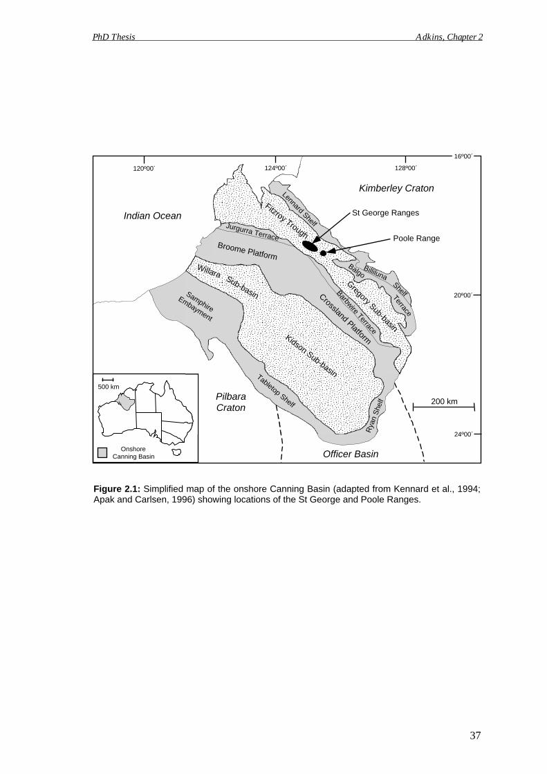
Figure 2.1: Simplified map of the onshore Canning Basin (adapted from Kennard et al., 1994;Apak and Carlsen, 1996) showing locations of the St George and Poole Ranges.
PhD Thesis Adkins, Chapter 2
Canning Basin
37
Noonkanbah FormationPoole Sandstone Measured Section
FaultSt George AnticlineQuaternary Sediments
Grant Group
Key
10 km
SG-1
18º40´
18º50´
125º00´ 125º10´ 125º20´4º50´
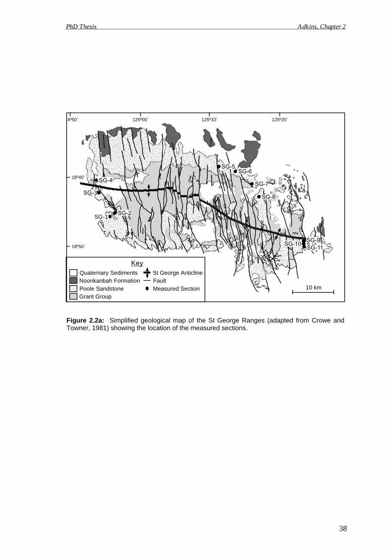
Figure 2.2a: Simplified geological map of the St George Ranges (adapted from Crowe andTowner, 1981) showing the location of the measured sections.
PhD Thesis Adkins, Chapter 2
38
10 km
Poole Sandstone Fault
Grant Group Measured Section
Poole AnticlineQuaternary Sediments
Key
125º50´
18º50´
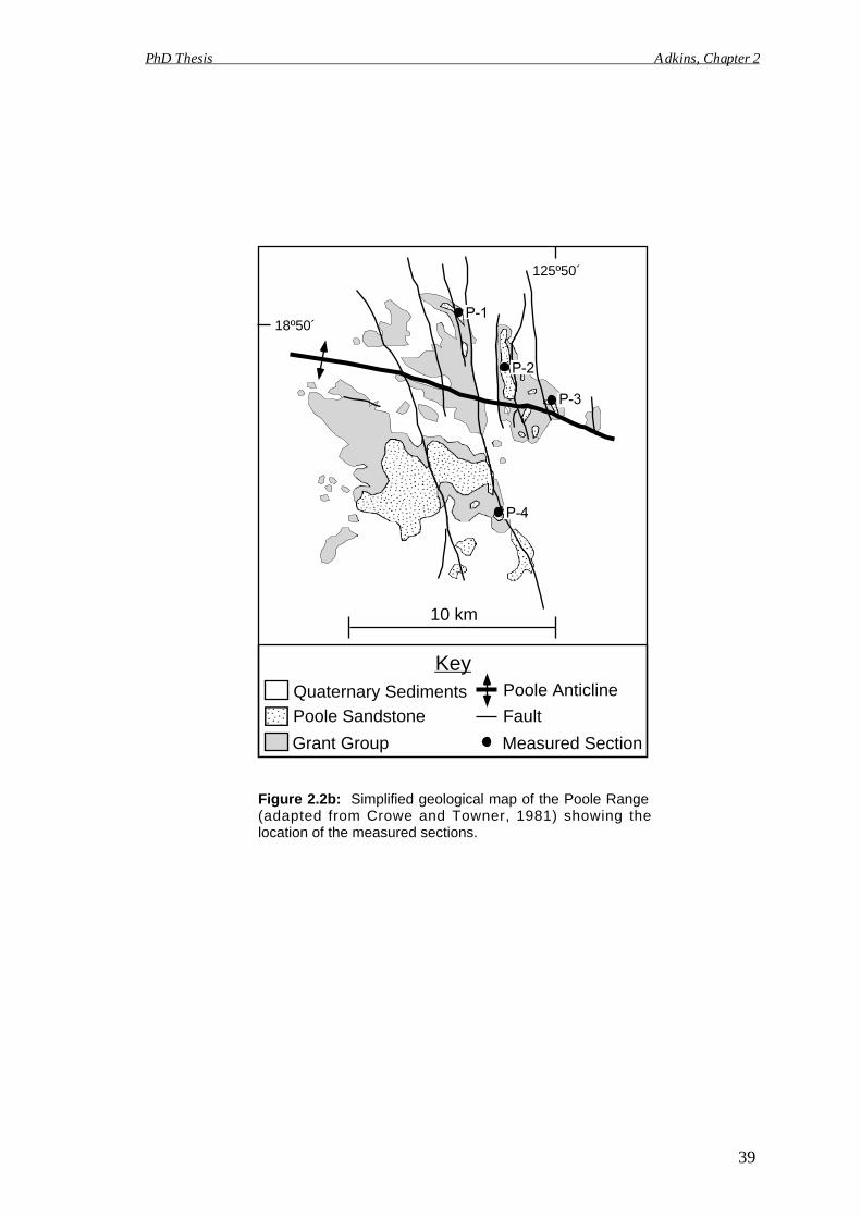
Figure 2.2b: Simplified geological map of the Poole Range(adapted from Crowe and Towner, 1981) showing thelocation of the measured sections.
PhD Thesis Adkins, Chapter 2
39
PhD Thesis Adkins, Chapter 2
40
GEOLOGIC SETTING
The onshore Canning Basin is the largest sedimentary basin in Western
Australia. It lies between the Proterozoic Kimberley Craton to the northeast and the
Archean Pilbara Craton to the southwest (Figure 2.1) (Purcell, 1984). Major northwest-
trending faults, controlled by terrane boundaries in underlying basement rock, define
the predominant structure of the basin (Hocking et al., 1994). Within the basin, two
northwest-trending depositional troughs, flanked by narrow shelves and terraces, are
separated by an uplifted mid-basin arch. The northern trough is divided by a basement
high into the Fitzroy Trough to the northwest and the Gregory Sub-basin to the
southeast. The southern trough is divided by a basement high into the Willara and
Kidson Sub-basins (Kennard et al., 1994).
Since the Early Ordovician, the Canning Basin has experienced four phases of
extension and transpression, each lasting approximately 70-80 million years. These
tectonic phases resulted in the deposition of four tectono-stratigraphic megasequences:
(i) Ordovician-Silurian; (ii) Devonian-Early Carboniferous; (iii) Late Carboniferous-
Permian; and (iv) Jurassic-Cretaceous (Kennard et al., 1994). Subsidence associated
with the Late Carboniferous-Permian megasequence was the most pronounced and
resulted in the deposition of a thick Permo-Carboniferous succession throughout the
basin. In the northern Fitzroy Trough, Late Carboniferous-Permian strata attain a
thickness of more than 4 km (Eyles and Eyles, 2000).
The St George and Poole Ranges of the Fitzroy Trough
Although deposits of the Late Carboniferous-Permian megasequence are
predominantly encountered in the sub-surface, a thick succession of Permian strata
outcrops in the highly-faulted, anticlinal St George and Poole Ranges of the Fitzroy
Trough (Figures 2.2 and 2.3). Strata from the St George and Poole Ranges record a
variety of glacially-influenced, shallow-marine to non-marine depositional
environments. These strata consist predominantly of siltstone and sandstone with only
minor amounts of finer and coarser grained sediment.
At the base of this succession, the Sakmarian Carolyn Formation (upper Grant
Group) is divided into the lower Wye Worry and upper Millajiddee Members (Crowe
and Towner, 1976a). The Wye Worry Member consists predominantly of calcareous
siltstone and sandy siltstone with locally abundant glacial dropstones (Crowe and
Towner, 1981). General characteristics of the Wye Worry Member suggest that it was
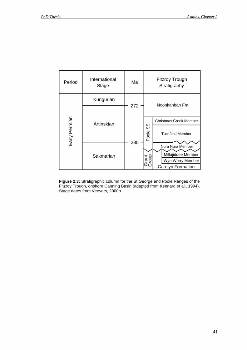
272
280
Fitzroy Trough
Noonkanbah Fm
Poo
le S
S
Christmas Creek Member
Nura Nura Member
Tuckfield Member
Kungurian
Artinskian
Sakmarian
InternationalMaPeriod
Ear
ly P
erm
ian
Carolyn Formation
Millajiddee Member
Wye Worry Member
Gra
ntG
roup
Figure 2.3: Stratigraphic column for the St George and Poole Ranges of theFitzroy Trough, onshore Canning Basin (adapted from Kennard et al., 1994).Stage dates from Veevers, 2000b.
PhD Thesis Adkins, Chapter 2
41
StratigraphyStage
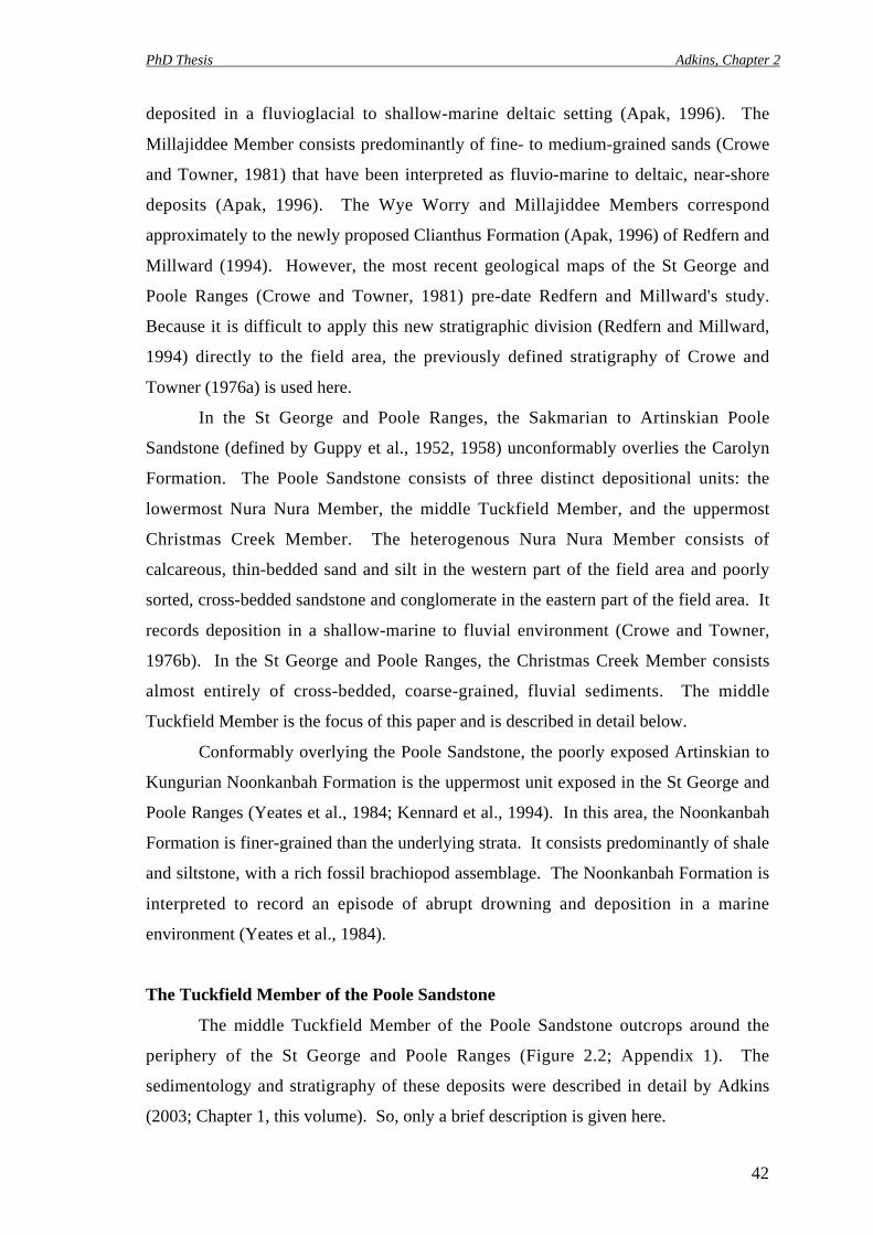
PhD Thesis Adkins, Chapter 2
42
deposited in a fluvioglacial to shallow-marine deltaic setting (Apak, 1996). The
Millajiddee Member consists predominantly of fine- to medium-grained sands (Crowe
and Towner, 1981) that have been interpreted as fluvio-marine to deltaic, near-shore
deposits (Apak, 1996). The Wye Worry and Millajiddee Members correspond
approximately to the newly proposed Clianthus Formation (Apak, 1996) of Redfern and
Millward (1994). However, the most recent geological maps of the St George and
Poole Ranges (Crowe and Towner, 1981) pre-date Redfern and Millward's study.
Because it is difficult to apply this new stratigraphic division (Redfern and Millward,
1994) directly to the field area, the previously defined stratigraphy of Crowe and
Towner (1976a) is used here.
In the St George and Poole Ranges, the Sakmarian to Artinskian Poole
Sandstone (defined by Guppy et al., 1952, 1958) unconformably overlies the Carolyn
Formation. The Poole Sandstone consists of three distinct depositional units: the
lowermost Nura Nura Member, the middle Tuckfield Member, and the uppermost
Christmas Creek Member. The heterogenous Nura Nura Member consists of
calcareous, thin-bedded sand and silt in the western part of the field area and poorly
sorted, cross-bedded sandstone and conglomerate in the eastern part of the field area. It
records deposition in a shallow-marine to fluvial environment (Crowe and Towner,
1976b). In the St George and Poole Ranges, the Christmas Creek Member consists
almost entirely of cross-bedded, coarse-grained, fluvial sediments. The middle
Tuckfield Member is the focus of this paper and is described in detail below.
Conformably overlying the Poole Sandstone, the poorly exposed Artinskian to
Kungurian Noonkanbah Formation is the uppermost unit exposed in the St George and
Poole Ranges (Yeates et al., 1984; Kennard et al., 1994). In this area, the Noonkanbah
Formation is finer-grained than the underlying strata. It consists predominantly of shale
and siltstone, with a rich fossil brachiopod assemblage. The Noonkanbah Formation is
interpreted to record an episode of abrupt drowning and deposition in a marine
environment (Yeates et al., 1984).
The Tuckfield Member of the Poole Sandstone
The middle Tuckfield Member of the Poole Sandstone outcrops around the
periphery of the St George and Poole Ranges (Figure 2.2; Appendix 1). The
sedimentology and stratigraphy of these deposits were described in detail by Adkins
(2003; Chapter 1, this volume). So, only a brief description is given here.
PhD Thesis Adkins, Chapter 2
43
In the St George and Poole Ranges, the Tuckfield Member consists of a series of
vertically stacked, coarsening- and thickening-upward cycles (Appendix 2). In outcrop,
these cycles are typically 7 to 12 m thick in the St George Ranges and 5 to 7 m thick in
the Poole Range, with some thinner cycles (2 to 4 m) observed at most locations. A
typical cycle consists upward of silty mudstone, siltstone, and sandstone. A supratidal,
mud-pellet and plant-fragment conglomerate often caps cycles in the western part of the
area (see Figures 2.4 and 2.5 for more detailed information). Primary sedimentary
structures, trace fossils and the vertical succession of facies suggest that each cycle
records an episode of shorezone progradation (Figure 2.4; Chapter 1, this volume).
Although the Tuckfield Member was probably deposited in less than 20 m of water
throughout the Fitzroy Trough (Brakel and Totterdell, 1993), relative cycle thicknesses
and the occurrence of supratidal deposits in the St George Ranges suggest that the Poole
Range records deposition in a slightly deeper, more shore-distal environment than the St
George Ranges.
Tuckfield Member cycles are laterally continuous in the field area. Flat-lying
benches usually correspond with cycle tops (Figure 2.6; Appendix 2). In Figures 2.5
and 2.7, heavy horizontal lines mark the tops of cycles. In Figure 2.7, eleven vertically
stacked, coarsening- and thickening-upward cycles are traced in the Poole Range for a
distance of over 10 km. Although Tuckfield Member cycles are also laterally
continuous in the St George Ranges, it is difficult to correlate the measured sections
from this area with absolute certainty. This difficulty can be attributed to the distance
between measured outcrops (typically 5 to 10 km), the limited variation of sedimentary
facies, and the highly faulted nature of the St George Ranges.
MILANKOVITCH THEORY AND THE ORBITAL PARAMETERS
Milankovitch theory is an astronomical theory of glaciation. It predicts that
fluctuations in the seasonal and geographic distribution of incident solar energy drive
climate change, the waxing and waning of glaciers, and therefore global sea-level (e.g.
Imbrie and Imbrie, 1979). Three orbital perturbations affect this distribution of incident
solar energy: eccentricity, obliquity, and precession (Figure 2.8). Eccentricity refers to
the shape of Earth's orbit around the sun, which varies from elliptical to near circular.
The period over which eccentricity varies from a maximum to a minimum and back is
approximately 100,000 years. A superimposed regular variation of eccentricity also
occurs at about 410,000 years. Obliquity refers to the angle of tilt in Earth's axis
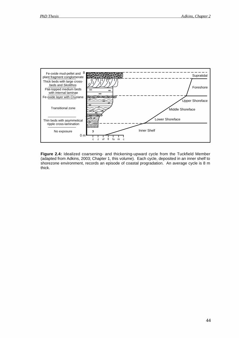
Foreshore
Upper Shoreface
Middle Shoreface
Lower Shoreface
Inner Shelf
Supratidal
?
8
0 mc z vf fl fu m c
Fe-oxide mud-pellet andplant fragment conglomerateThick beds with large cross-
beds and SkolithosFlat-topped medium beds
with internal laminaeFe-oxide layer with Cruziana
Transitional zone
Thin beds with asymmeticalripple cross-lamination
No exposure
Figure 2.4: Idealized coarsening- and thickening-upward cycle from the Tuckfield Member(adapted from Adkins, 2003; Chapter 1, this volume). Each cycle, deposited in an inner shelf toshorezone environment, records an episode of coastal progradation. An average cycle is 8 mthick.
PhD Thesis Adkins, Chapter 2
44
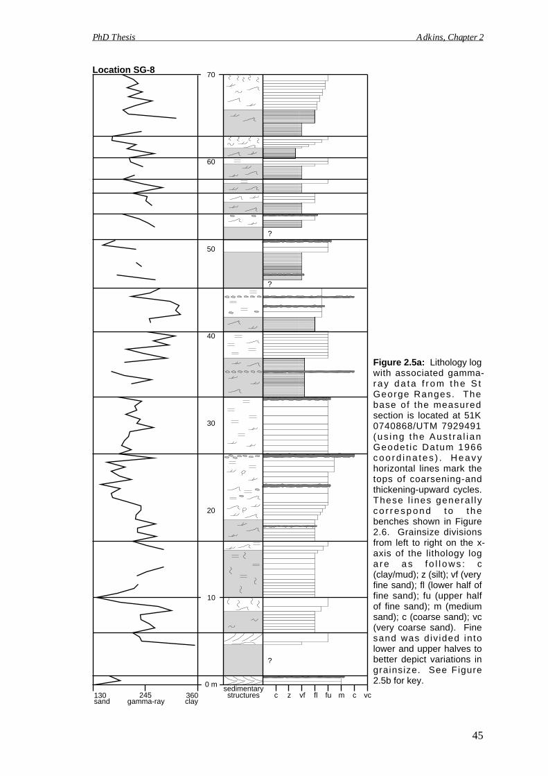
30
60
20
40
50
?
?
?
130 360245sand gamma-ray clay
sedimentarystructures c z vf fl fu m c vc
0 m
70Location SG-8
Figure 2.5a: Lithology logwith associated gamma-r a y d a t a f r o m t h e S tGeorge Ranges. Thebase of the measuredsection is located at 51K0740868/UTM 7929491(us ing the Aus t ra l i anGeodet ic Datum 1966coo rd i na tes ) . Heavyhorizontal lines mark thetops of coarsening-andthickening-upward cycles.These l ines genera l lyc o r r e s p o n d t o t h ebenches shown in Figure2.6. Grainsize divisionsfrom left to right on the x-axis of the lithology loga r e a s f o l l o w s : c(clay/mud); z (silt); vf (veryfine sand); fl (lower half offine sand); fu (upper halfof fine sand); m (mediumsand); c (coarse sand); vc(very coarse sand). Finesand was d iv ided in tolower and upper halves tobetter depict variations ingrainsize. See Figure2.5b for key.
10
PhD Thesis Adkins, Chapter 2
45
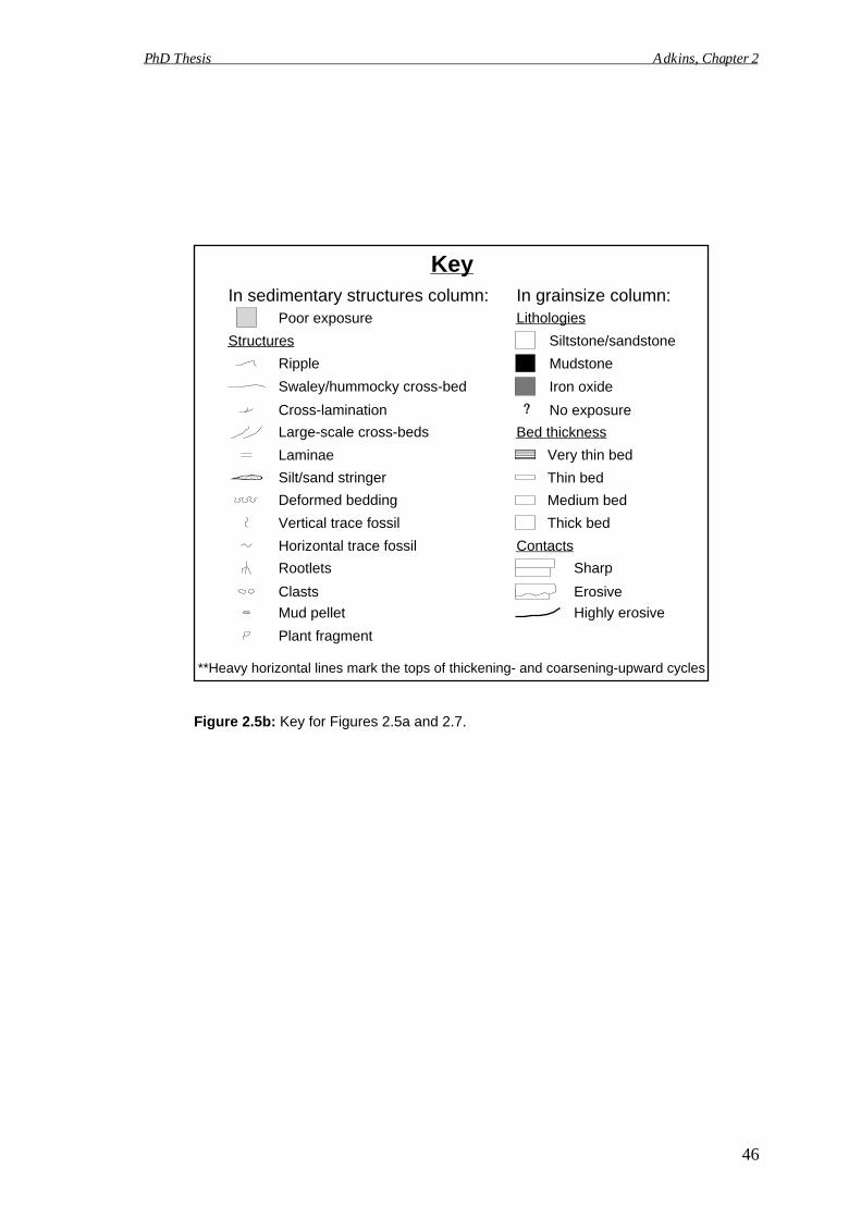
MudstoneRipple
Swaley/hummocky cross-bed Iron oxide
Cross-lamination No exposure
Silt/sand stringer Thin bed
Laminae Very thin bed
Horizontal trace fossil Contacts
Vertical trace fossil Thick bed
Plant fragment
Clasts Erosive
Rootlets Sharp
Mud pellet Highly erosive
Large-scale cross-beds Bed thickness
Poor exposure Lithologies
Siltstone/sandstoneStructures
In grainsize column:In sedimentary structures column:
Medium bedDeformed bedding
Key
**Heavy horizontal lines mark the tops of thickening- and coarsening-upward cycles
Figure 2.5b: Key for Figures 2.5a and 2.7.
PhD Thesis Adkins, Chapter 2
46
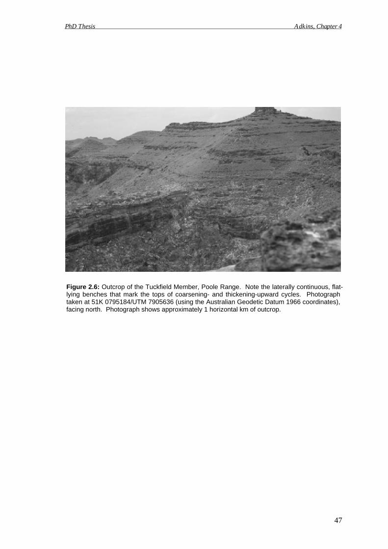
PhD Thesis Adkins, Chapter 4
47
Figure 2.6: Outcrop of the Tuckfield Member, Poole Range. Note the laterally continuous, flat-lying benches that mark the tops of coarsening- and thickening-upward cycles. Photographtaken at 51K 0795184/UTM 7905636 (using the Australian Geodetic Datum 1966 coordinates),facing north. Photograph shows approximately 1 horizontal km of outcrop.
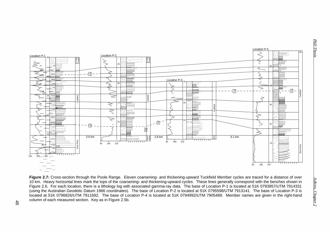
?
Nu
raN
ura
?
??
??
Location P-150
40
30
20
10
0 m100 200 300
?
?
Nur
a N
ura
X-m
asC
reek
3.6 km 2.8 km
Location P-3
Location P-2
6.1 km
Location P-4
31020090
40
30
20
10
0 m
?
?
Nur
aN
ura
X-m
asC
reek
30
20
10
0 m51030090
?
?
50
40
30
20
10
0 m37023090
?
?
?
?
Nur
a N
ura
?
X
Tuc
kfie
ld
Tuc
kfie
ld
Tuc
kfie
ld
Tuc
kfie
ld
Figure 2.7: Cross-section through the Poole Range. Eleven coarsening- and thickening-upward Tuckfield Member cycles are traced for a distance of over10 km. Heavy horizontal lines mark the tops of the coarsening- and thickening-upward cycles. These lines generally correspond with the benches shown inFigure 2.6. For each location, there is a lithology log with associated gamma-ray data. The base of Location P-1 is located at 51K 0793957/UTM 7914331(using the Australian Geodetic Datum 1966 coordinates). The base of Location P-2 is located at 51K 0795598/UTM 7913141. The base of Location P-3 islocated at 51K 0796826/UTM 7911692. The base of Location P-4 is located at 51K 0794992/UTM 7905489. Member names are given in the right-handcolumn of each measured section. Key as in Figure 2.5b.
PhD T
hesis
Adkins, C
hapter 2
31
48
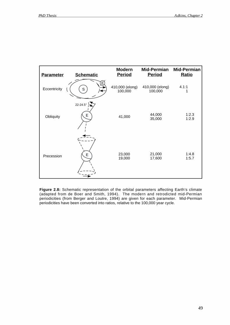
E
E
Eccentricity
Obliquity
Precession
410,000 (elong)100,000
4.1:11
1:2.31:2.9
1:4.81:5.7
44,00035,000
21,00017,600
Mid-Permian Mid-PermianParameter Schematic
E
S
Modern
410,000 (elong)100,000
41,000
23,00019,000
22-24.5°
Figure 2.8: Schematic representation of the orbital parameters affecting Earth’s climate(adapted from de Boer and Smith, 1994). The modern and retrodicted mid-Permianperiodicities (from Berger and Loutre, 1994) are given for each parameter. Mid-Permianperiodicities have been converted into ratios, relative to the 100,000 year cycle.
PhD Thesis Adkins, Chapter 2
49
Period Period Ratio
PhD Thesis Adkins, Chapter 2
50
relative to the plane in which it rotates around the Sun. Obliquity varies between 22º
and 24.5º and has a modern period of approximately 41,000 years. Precession refers to
the wobble of Earth's axis of rotation that follows a roughly cone-shaped envelope. The
modern precessional period is approximately 26,000 years with dual components of
23,000 and 19,000 years. For a more detailed review of the orbital parameters, see:
Imbrie and Imbrie, 1979; Imbrie, 1985; Schwarzacher, 1993; or House, 1995.
The astronomical periods listed above are for the present. Berger and Loutre
(1994) demonstrated that these values have changed throughout time. The astronomical
periods for precession and obliquity have slowly lengthened during the past 2.5 billion
years. This can be partially attributed to the combined lengthening of the Earth-Moon
distance and the lengthening of the average day (Lambeck, 1980). Two hundred
seventy (270) Ma (mid-Permian), obliquity had a periodicity with dual components of
approximately 44,000 and 35,000 years. Precession had a periodicity with dual
components of approximately 21,000 and 17,600 years (Figure 2.8). Eccentricity is not
influenced by these variations. Therefore, the periods of eccentricity and elongated
eccentricity (100,000 and 410,000 years) have remained relatively constant (Berger and
Loutre, 1994).
SPECTRAL ANALYSIS
Spectral analysis is an objective, statistical method that can detect regular
cyclicity in a dataset (Weedon, 1991). Although much speculation preceded their work,
Hays et al. (1976) were the first to use spectral analysis to demonstrate that major
climatic changes can be directly linked to variations in Earth's orbital parameters. This
was achieved by identifying periodicities in oxygen isotope data (from planktonic
foraminifera) that are consistent with the known periodicities of eccentricity, obliquity,
and precession. Since that pivotal study, spectral analysis has been used to identify
orbitally-induced, climatic variations recorded throughout the stratigraphic column
(Reijmer et al., 1994; Weedon and Read, 1995; Weedon et al., 1999; Sierro et al.,
2000).
In this study, gamma-ray data from each measured outcrop were analyzed using
two spectral analysis programs (Appendices 9 and 10). Spectral plots generated from
analysis of gamma-ray data from Location SG-8 are presented in Figure 2.9. In both
plots (Figures 2.9a and 2.9b), spectral peaks represent cycles recorded in the rock
record. The reciprocal of the frequency for each peak is equal to the average period of
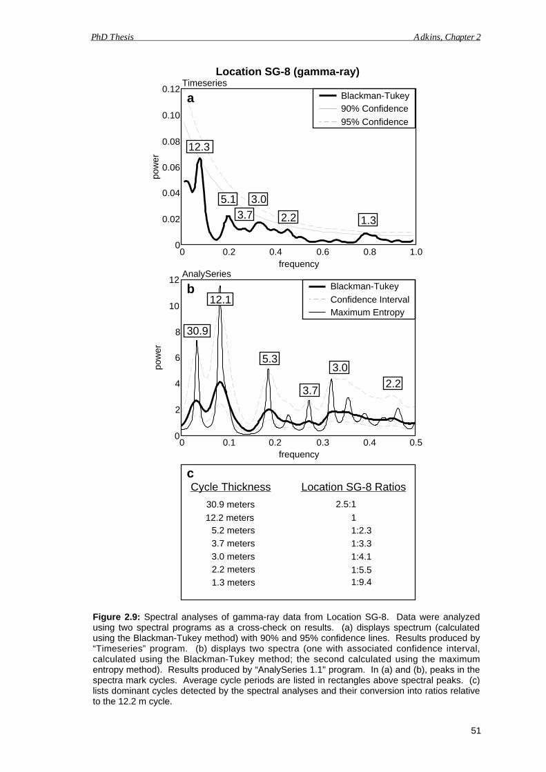
0.50.40.30.20.100
12Blackman-Tukey
Confidence Interval
frequency
pow
er
AnalySeries
10
8
6
4
2
Maximum Entropy12.1
3.7
30.9
5.33.0
2.2
b
0 0.2 0.4 0.6 0.8 1.00
0.06
0.10
0.12Blackman-Tukey90% Confidence
95% Confidence
frequency
pow
er
Timeseries
0.08
0.04
0.02
12.3
5.1
1.32.2
3.0
3.7
a
Cycle Thickness
30.9 meters
12.2 meters
3.0 meters
3.7 meters
1.3 meters
2.2 meters
1:3.3
1:4.1
1:5.51:9.4
5.2 meters
Location SG-8 Ratios
2.5:1
11:2.3
c
Location SG-8 (gamma-ray)
Figure 2.9: Spectral analyses of gamma-ray data from Location SG-8. Data were analyzedusing two spectral programs as a cross-check on results. (a) displays spectrum (calculatedusing the Blackman-Tukey method) with 90% and 95% confidence lines. Results produced by“Timeseries” program. (b) displays two spectra (one with associated confidence interval,calculated using the Blackman-Tukey method; the second calculated using the maximumentropy method). Results produced by “AnalySeries 1.1" program. In (a) and (b), peaks in thespectra mark cycles. Average cycle periods are listed in rectangles above spectral peaks. (c)lists dominant cycles detected by the spectral analyses and their conversion into ratios relativeto the 12.2 m cycle.
PhD Thesis Adkins, Chapter 2
51
PhD Thesis Adkins, Chapter 2
52
that cycle in meters (shown in rectangles above spectral peaks). Spectral peaks
generated by the two programs were compared, averaged, and used to determine the
periodicities of all significant cycles recorded at each location. For Location SG-8,
cycles with periodicities of 30.9 m, 12.2 m, 5.2 m, 3.7 m, 3.0 m, 2.2 m and 1.3 m were
detected (Figure 2.9c).
As a further check on the results, a similar process was performed on grainsize
data from each measured outcrop (Appendices 9 and 11). Spectral plots generated from
the analysis of grainsize data from Location SG-8 are presented in Figures 2.10a and
2.10b. Cycles with periodicities of 48.3 m, 13.9 m, 5.7 m, 4.6 m, 3.3 m, 2.4 m, 1.9 m
and 1.6 m were detected (Figure 2.10c).
Table 2.1 summarizes the results of all spectral analyses performed in this study.
The table is organized in a manner that will allow easy comparison of the detected
periodicities from the 15 measured sections. This table is also organized to allow a
comparison between the results presented here and the results presented in Tables 2.2-
2.4, which will be discussed later in the text. Detected cycles can be grouped into six
main categories/columns that are labeled A through F in Table 2.1. Additional cycles
were detected in some datasets. They are listed in columns labeled 1 through 4.
In Table 2.1, periodicities detected from the analysis of gamma-ray data are
listed in plain text. Periodicities detected from the analysis of grainsize data are listed
in bold text. For most outcrops, periodicities from grainsize data compare favorably
with periodicities from gamma-ray data. The largest discrepancies occur in Column A
(e.g. Location SG-10), where cycles with the longest periods are listed. These
discrepancies are probably related to the total length of the measured sections. Because
spectral programs search for repetitive cycles, they cannot accurately detect
periodicities greater than about half the total length of the dataset. Since the outcrops in
this study range between 30 and 110 m thick, many of the periodicities listed in Column
A are approaching the spectral programs' upper limit of detection. This may have
resulted in some erroneous spectral peaks.
In addition to a favorable comparison between the gamma-ray and grainsize
periods for each outcrop, the results from the 15 different locations also compare
favorably with one another. In Column B (Table 2.1), most of the detected periodicities
fall within a limited range. One notable observation is the difference in periodicities
from the two areas. In the St George Ranges, the periodicities listed in Column B range
between 7.4 m and 13.9 m with an average thickness of 10.9 m. In the Poole Range, the
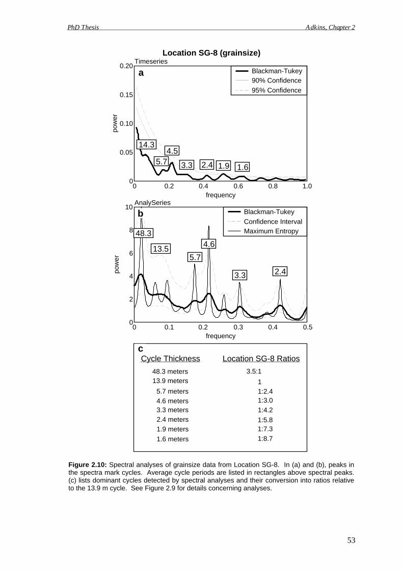
0.50.40.30.20.100
2
4
6
8
10Blackman-Tukey
Confidence Interval
frequency
pow
er
AnalySeries
Maximum Entropy
13.54.6
48.3
5.7
2.43.3
b
0 0.2 0.4 0.6 0.8 1.00
0.05
0.10
0.15
0.20Blackman-Tukey90% Confidence
95% Confidence
frequency
pow
er
Timeseries
14.3
5.71.61.92.43.3
4.5
a
Location SG-8 (grainsize)
Cycle Thickness
48.3 meters13.9 meters
3.3 meters
1.9 meters
2.4 meters1:4.2
1:5.81:7.3
1:8.7
4.6 meters
5.7 meters
Location SG-8 Ratios
3.5:1
11:2.41:3.0
1.6 meters
c
Figure 2.10: Spectral analyses of grainsize data from Location SG-8. In (a) and (b), peaks inthe spectra mark cycles. Average cycle periods are listed in rectangles above spectral peaks.(c) lists dominant cycles detected by spectral analyses and their conversion into ratios relativeto the 13.9 m cycle. See Figure 2.9 for details concerning analyses.
PhD Thesis Adkins, Chapter 2
53
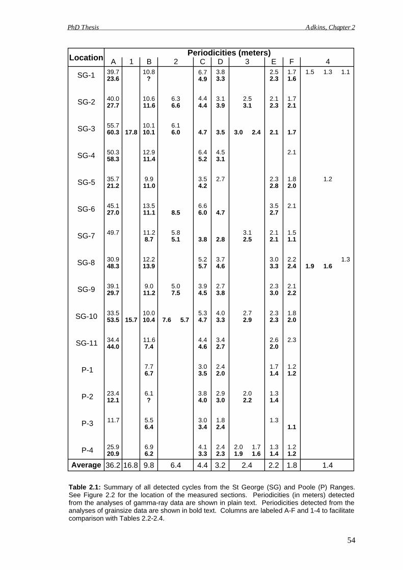
P-4
P-1
P-2
P-3
SG-11
SG-10
SG-9
SG-8
SG-7
SG-6
SG-5
SG-2
SG-3
SG-4
SG-1
Location A B C D E FPeriodicities (meters)
39.723.6
10.8?
6.74.9
3.83.3
2.52.3
1.71.6
1.5 1.3 1.1
40.027.7
10.611.6
6.36.6
4.44.4
3.13.9
2.53.1
2.12.3
1.72.1
55.760.3 17.8
10.110.1
6.16.0 4.7 3.5 3.0 2.4 2.1 1.7
50.358.3
12.911.4
6.45.2
4.53.1
2.1
35.721.2
9.911.0
3.54.2
2.7 2.32.8
1.82.0
1.2
45.127.0
13.511.1 8.5
6.66.0 4.7
3.52.7
2.1
49.7 11.28.7
5.85.1 3.8 2.8
3.12.5
2.12.1
1.51.1
30.948.3
12.213.9
5.25.7
3.74.6
3.03.3
2.22.4 1.9 1.6
1.3
39.129.7
9.011.2
5.07.5
3.94.5
2.73.8
2.33.0
2.12.2
33.553.5 15.7
10.010.4 7.6 5.7
5.34.7
4.03.3
2.72.9
2.32.3
1.82.0
34.444.0
11.67.4
4.44.6
3.42.7
2.62.0
2.3
7.76.7
3.03.5
2.42.0
1.71.4
1.21.2
23.412.1
6.1?
3.84.0
2.93.0
2.02.2
1.31.4
11.7 5.56.4
3.03.4
1.82.4
1.31.1
25.920.9
6.96.2
4.13.3
2.42.3
2.01.9
1.71.6
1.31.4
1.21.2
1 2 3 4
Average 36.2 16.8 9.8 4.4 3.2 2.2 1.86.4 2.4 1.4
Table 2.1: Summary of all detected cycles from the St George (SG) and Poole (P) Ranges.See Figure 2.2 for the location of the measured sections. Periodicities (in meters) detectedfrom the analyses of gamma-ray data are shown in plain text. Periodicities detected from theanalyses of grainsize data are shown in bold text. Columns are labeled A-F and 1-4 to facilitatecomparison with Tables 2.2-2.4.
PhD Thesis Adkins, Chapter 2
54
PhD Thesis Adkins, Chapter 2
55
detected periodicities range between 5.5 m and 7.7 m with an average thickness of 6.5
m. Columns C through F show similar relationships with thinner cycles noted in the
Poole Range than in the St George Ranges.
A COMPARISON OF CYCLICITY
To test for a glacio-eustatic driving mechanism, cycles detected in the Tuckfield
Member (Table 2.1) were compared to the known mid-Permian orbital parameters
(Figure 2.8). Since the periodicities of the Tuckfield cycles are spatial (given in meters)
and the periodicities of the orbital parameters are temporal (given in years), a direct
comparison could not be made. To effectively compare the two, all sets of periodicities
had to be converted into sets of ratios.
Table 2.2 summarizes the conversion of the periodicities detected from the
analysis of gamma-ray data into ratios. For this conversion, cycle periodicities in
Column B (Table 2.1) were set to one (Table 2.2). Detected periodicities in each
dataset were converted into ratios relative to the associated Column B periodicity (Table
2.1). For example, at Location SG-1 the cycle periodicity listed in column B is 10.8 m.
The cycle periodicity listed in Column C is 6.7 m (Table 2.1). Since the number of 6.7
m cycles (Column C) in each 10.8 m cycle (Column B) equals 1.6 (10.8 ÷ 6.7 = 1.6),
the Column C ratio in Table 2.2 for Location SG-1 is 1:1.6. At the base of Table 2.2,
the average ratio for each column is given.
Table 2.3 summarizes the conversion of the periodicities detected from the
analysis of grainsize data into ratios, using the above method. Again, the average ratios
for each column is given at the base of the table.
The orbital parameters were converted into ratios by setting the 100,000 year
cycle equal to one. For example, the number of 17,600 year cycles in each 100,000
year cycle is equal to 5.7 (100,000 ÷ 17,600 = 5.7). Therefore, the ratio used for the
17,600 year cycle is 1:5.7. The complete listing of Milankovitch ratios is given in
Figure 2.8.
Table 2.4 lists the average gamma-ray ratios, the average grainsize ratios, and
the ratios for the mid-Permian orbital parameters. These three sets of results compare
favorably with one another. There is also a favorable comparison between the gamma-
ray ratios and the grainsize ratios for the "extra," non-Milankovitch-band periodicities
(Table 2.4).
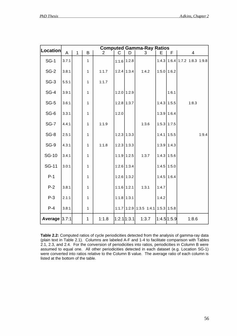
P-4 3.8:1 1 1:1.7 1:2.9 1:3.5 1:4.1 1:5.3 1:5.8
P-1 1 1:2.6 1:3.2 1:4.5 1:6.4
P-2 3.8:1 1 1:1.6 1:2.1 1:3.1 1:4.7
P-3 2.1:1 1 1:1.8 1:3.1 1:4.2
SG-11 3.0:1 1 1:2.6 1:3.4 1:4.5 1:5.0
SG-10 3.4:1 1 1:1.9 1:2.5 1:3.7 1:4.3 1:5.6
SG-9 4.3:1 1 1:1.8 1:2.3 1:3.3 1:3.9 1:4.3
SG-8 2.5:1 1 1:2.3 1:3.3 1:4.1 1:5.5 1:9.4
SG-7 4.4:1 1 1:1.9 1:3.6 1:5.3 1:7.5
SG-6 3.3:1 1 1:2.0 1:3.9 1:6.4
SG-5 3.6:1 1 1:2.8 1:3.7 1:4.3 1:5.5 1:8.3
SG-2 3.8:1 1 1:1.7 1:2.4 1:3.4 1:4.2 1:5.0 1:6.2
SG-3 5.5:1 1 1:1.7
SG-4 3.9:1 1 1:2.0 1:2.9 1:6.1
SG-1 3.7:1 1 1:1.6 1:2.8 1:4.3 1:6.4 1:7.2 1:8.3 1:9.8
Location A B C D E FComputed Gamma-Ray Ratios
Average 3.7:1 1 1:1.8 1:2.11:3.1 1:3.7 1:4.5 1:5.9 1:8.6
1 2 3 4
Table 2.2: Computed ratios of cycle periodicities detected from the analysis of gamma-ray data(plain text in Table 2.1). Columns are labeled A-F and 1-4 to facilitate comparison with Tables2.1, 2.3, and 2.4. For the conversion of periodicities into ratios, periodicities in Column B wereassumed to equal one. All other periodicities detected in each dataset (e.g. Location SG-1)were converted into ratios relative to the Column B value. The average ratio of each column islisted at the bottom of the table.
PhD Thesis Adkins, Chapter 2
56
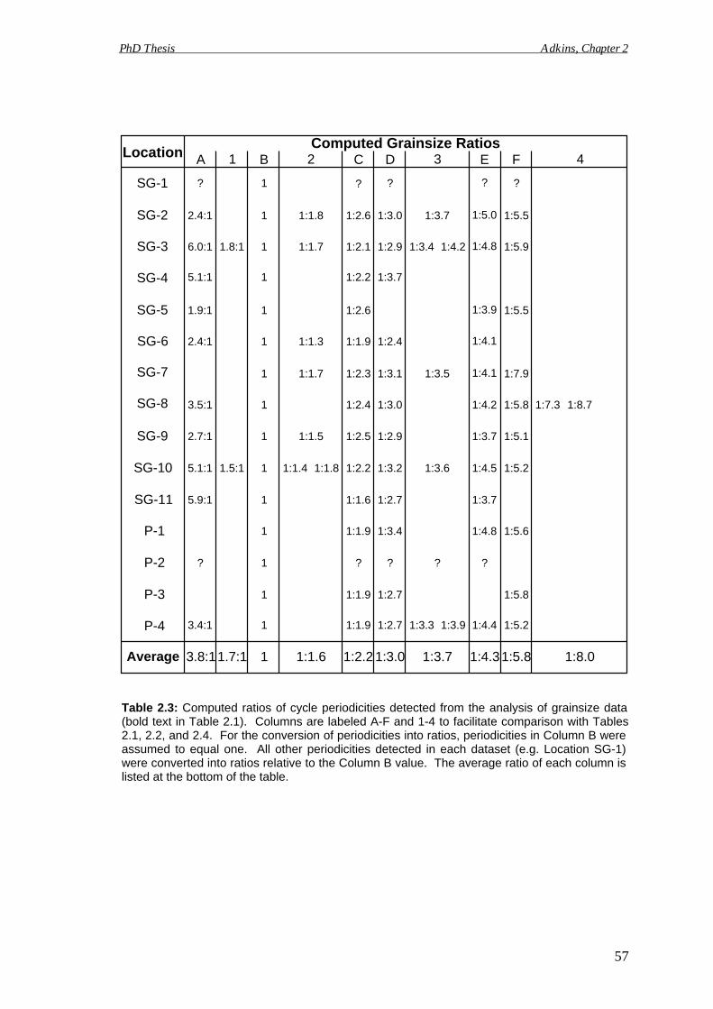
P-4 3.4:1 1 1:1.9 1:2.7 1:3.3 1:3.9 1:4.4 1:5.2
P-1 1 1:1.9 1:3.4 1:4.8 1:5.6
P-2 ? 1 ? ? ? ?
P-3 1 1:1.9 1:2.7 1:5.8
SG-11 5.9:1 1 1:1.6 1:2.7 1:3.7
SG-10 5.1:1 1.5:1 1 1:1.4 1:1.8 1:2.2 1:3.2 1:3.6 1:4.5 1:5.2
SG-9 2.7:1 1 1:1.5 1:2.5 1:2.9 1:3.7 1:5.1
SG-8 3.5:1 1 1:2.4 1:3.0 1:4.2 1:5.8 1:7.3 1:8.7
SG-7 1 1:1.7 1:2.3 1:3.1 1:3.5 1:4.1 1:7.9
SG-6 2.4:1 1 1:1.3 1:1.9 1:2.4 1:4.1
SG-5 1.9:1 1 1:2.6 1:3.9 1:5.5
SG-2 2.4:1 1 1:1.8 1:2.6 1:3.0 1:3.7 1:5.0 1:5.5
SG-3 6.0:1 1.8:1 1 1:1.7 1:2.1 1:2.9 1:3.4 1:4.2 1:4.8 1:5.9
SG-4 5.1:1 1 1:2.2 1:3.7
SG-1 ? 1 ? ? ? ?
Location A B C D E FComputed Grainsize Ratios
Average 3.8:11.7:1 1 1:1.6 1:2.2 1:3.0 1:3.7 1:4.31:5.8 1:8.0
1 2 3 4
Table 2.3: Computed ratios of cycle periodicities detected from the analysis of grainsize data(bold text in Table 2.1). Columns are labeled A-F and 1-4 to facilitate comparison with Tables2.1, 2.2, and 2.4. For the conversion of periodicities into ratios, periodicities in Column B wereassumed to equal one. All other periodicities detected in each dataset (e.g. Location SG-1)were converted into ratios relative to the Column B value. The average ratio of each column islisted at the bottom of the table.
PhD Thesis Adkins, Chapter 2
57
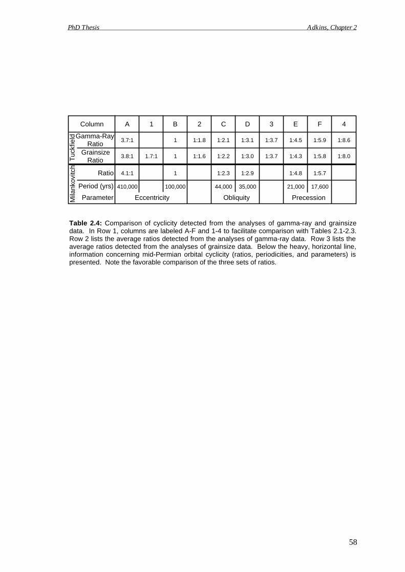
Gamma-Ray
Grainsize
Mila
nkov
itch
Parameter Eccentricity Obliquity Precession
Period (yrs)
Ratio 4.1:1 1 1:2.3 1:2.9 1:4.8 1:5.7
17,60021,00035,00044,000100,000410,000
3.8:1 1.7:1 1 1:1.6 1:2.2 1:3.0 1:3.7 1:4.3 1:5.8 1:8.0
1:8.61:5.91:4.51:3.71:3.11:2.11:1.813.7:1
Tuc
kfie
ld
Column A B1 2 C D 3 E F 4
Table 2.4: Comparison of cyclicity detected from the analyses of gamma-ray and grainsizedata. In Row 1, columns are labeled A-F and 1-4 to facilitate comparison with Tables 2.1-2.3.Row 2 lists the average ratios detected from the analyses of gamma-ray data. Row 3 lists theaverage ratios detected from the analyses of grainsize data. Below the heavy, horizontal line,information concerning mid-Permian orbital cyclicity (ratios, periodicities, and parameters) ispresented. Note the favorable comparison of the three sets of ratios.
PhD Thesis Adkins, Chapter 2
58
Ratio
Ratio

PhD Thesis Adkins, Chapter 2
59
DISCUSSION
The favorable comparison between the Tuckfield Member cycles and the mid-
Permian orbital parameters indicates that orbital cyclicity was probably the driving
force in the formation of the Tuckfield Member cycles. However, this positive
correlation does not necessarily mean that the Tuckfield Member cycles are glacio-
eustatic in origin. For example, Fielding and Webb (1996) used spectral analysis to
identify Milankovitch-scale cyclicity in Late Permian alluvial deposits from the
Bainmedart Coal Measures in Antarctica. They attributed the observed cyclicity to
changing sediment supply that was controlled by orbitally-forced climate change, not
glacio-eustatic sea-level fluctuations.
Although the Bainmedart Coal Measures record Milankovitch-scale cyclicity
and are similar in age to the Tuckfield Member, these deposits cannot be used as a
direct analog. The depositional environment of the two areas are too dissimilar for a
worthwhile comparison. To gain a better understanding of the Tuckfield Member
cycles, it is best to compare them with other mid- to Late Permian shallow-marine,
cyclic deposits (Table 2.5). The number of publications documenting such deposits are
extremely limited. Three notable exceptions are considered here (Table 2.5).
In Australia, the Artinskian to Ufimian Pebbley Beach Formation of the
southern Sydney Basin consists of a series of coarsening-upward, shallow-marine,
siliciclastic cycles (Chapter 5, this volume). Spectral analysis of gamma-ray data from
the Pebbley Beach Formation reveals several orders of cyclicity, with periodicities of
8.5 m, 4.9 m, 3.2 m, 1.8 m and 1.3 m (Table 2.5). These Pebbley Beach cycles have
been attributed to changes in eccentricity (8.5 m cycle), obliquity (4.9 and 3.2 m
cycles), and precession (1.8 and 1.3 m cycles).
The Upper Guadalupian (latest Permian) Yates Formation of the Permian Basin
(USA) consists of a series of outer- to inner-shelf, alternating carbonate/siliciclastic
cycles. Borer and Harris (1991) utilized Fischer plots and spectral analysis to constrain
cyclicity within this unit. They identified large-scale (30 m) cycles that contained 4
smaller-scale cycles of varying thickness. The 30 m cycles were interpreted to be
400,000 year eccentricity cycles, whereas the smaller-scale cycles were interpreted to be
100,000 year eccentricity cycles (Table 2.5).
At the Permo-Triassic boundary, the Gartnerkofel section from the Carnic Alps
in Austria consists of dolomitized limestone and interbedded thin marls and shales of
shallow-marine origin (Rampino et al., 2000). Spectral analysis of gamma-ray data
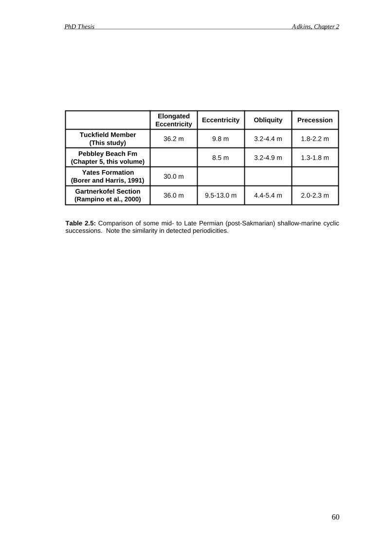
ElongatedEccentricity Obliquity Precession
Tuckfield Member
Pebbley Beach Fm
Yates Formation
Gartnerkofel Section
36.2 m
30.0 m
36.0 m
9.8 m
8.5 m
9.5-13.0 m
3.2-4.4 m
3.2-4.9 m
4.4-5.4 m
1.8-2.2 m
1.3-1.8 m
2.0-2.3 m
Table 2.5: Comparison of some mid- to Late Permian (post-Sakmarian) shallow-marine cyclicsuccessions. Note the similarity in detected periodicities.
PhD Thesis Adkins, Chapter 2
60
(This study)
(Chapter 5, this volume)
(Borer and Harris, 1991)
(Rampino et al., 2000)
Eccentricity
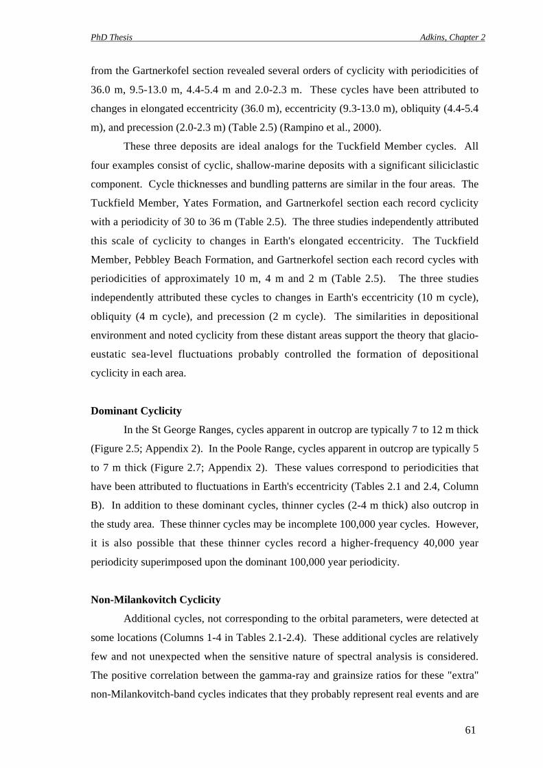
PhD Thesis Adkins, Chapter 2
from the Gartnerkofel section revealed several orders of cyclicity with periodicities of
36.0 m, 9.5-13.0 m, 4.4-5.4 m and 2.0-2.3 m. These cycles have been attributed to
changes in elongated eccentricity (36.0 m), eccentricity (9.3-13.0 m), obliquity (4.4-5.4
m), and precession (2.0-2.3 m) (Table 2.5) (Rampino et al., 2000).
These three deposits are ideal analogs for the Tuckfield Member cycles. All
four examples consist of cyclic, shallow-marine deposits with a significant siliciclastic
component. Cycle thicknesses and bundling patterns are similar in the four areas. The
Tuckfield Member, Yates Formation, and Gartnerkofel section each record cyclicity
with a periodicity of 30 to 36 m (Table 2.5). The three studies independently attributed
this scale of cyclicity to changes in Earth's elongated eccentricity. The Tuckfield
Member, Pebbley Beach Formation, and Gartnerkofel section each record cycles with
periodicities of approximately 10 m, 4 m and 2 m (Table 2.5). The three studies
independently attributed these cycles to changes in Earth's eccentricity (10 m cycle),
obliquity (4 m cycle), and precession (2 m cycle). The similarities in depositional
environment and noted cyclicity from these distant areas support the theory that glacio-
eustatic sea-level fluctuations probably controlled the formation of depositional
cyclicity in each area.
Dominant Cyclicity
In the St George Ranges, cycles apparent in outcrop are typically 7 to 12 m thick
(Figure 2.5; Appendix 2). In the Poole Range, cycles apparent in outcrop are typically 5
to 7 m thick (Figure 2.7; Appendix 2). These values correspond to periodicities that
have been attributed to fluctuations in Earth's eccentricity (Tables 2.1 and 2.4, Column
B). In addition to these dominant cycles, thinner cycles (2-4 m thick) also outcrop in
the study area. These thinner cycles may be incomplete 100,000 year cycles. However,
it is also possible that these thinner cycles record a higher-frequency 40,000 year
periodicity superimposed upon the dominant 100,000 year periodicity.
Non-Milankovitch Cyclicity
Additional cycles, not corresponding to the orbital parameters, were detected at
some locations (Columns 1-4 in Tables 2.1-2.4). These additional cycles are relatively
few and not unexpected when the sensitive nature of spectral analysis is considered.
The positive correlation between the gamma-ray and grainsize ratios for these "extra"
non-Milankovitch-band cycles indicates that they probably represent real events and are
61

PhD Thesis Adkins, Chapter 2
not simply erroneous peaks in the spectral plots. These "extra" cycles may record
localized tectonic activity or short- to long-term changes in sediment supply.
The Stratigraphic Effects of Deglaciation
Eyles and Eyles have published several recent papers on the Permo-
Carboniferous system of Australia (e.g. Eyles et al., 1997; Eyles et al., 1998; Eyles et
al., 2001; Eyles and Eyles, 2000). Much of their work has focused on the development
of large-scale, 30+ million-year, diamictite/shale/sandstone sequences that occur
throughout Western Australia (e.g. Eyles et al., 2002; Eyles et al., 2003). Within these
sequences, the lowermost diamictite succession is typically composed of rapidly
deposited, glacially influenced, marine strata. The middle succession typically consists
of fossiliferous cool water shales. The upper sandstone succession typically comprises
shallow marine, wave- and storm-influenced sandstone (Eyles et al., 2002; Eyles et al.,
2003).
These studies suggest that tectonism, not glacio-eustacy, is responsible for the
formation of the observed sequences. In their model, the lower diamictite part of the
sequence records basin infilling of coarse debris produced by faulting and glaciation of
the adjacent craton. The middle shale part of the sequence marks a phase of sediment
under-filling, characterized by tectonic subsidence, an increase in relative sea-level, and
a reduction in sediment supply. The upper sandstone part of the sequence records a late
stage in the tectonic cycle when subsidence rates have decreased and sediment supply
overcomes accommodation space (Eyles et al., 2002; Eyles et al., 2003).
In the Canning Basin, the upper sandstone unit of Eyles and Eyles’ tripartite
sequence consists of the Clianthus Formation (i.e. Wye Worry and Millajiddee
Members), the Poole Sandstone, and the Noonkanbah Formation (Eyles et al., 2002).
As discussed earlier, these are the rocks that outcrop in the St George and Poole
Ranges. These strata appear to provide a direct record of Permian deglaciation
superimposed upon the larger, tectonic sequence described by Eyles et al. (2002).
During the earliest Permian, continental ice covered much of Australia.
Palynological analysis indicates that the glacial climax was reached in the northern
regions of Western Australia (Pilbara Craton) during the Sakmarian (Crowell and
Frakes, 1971). In the Canning Basin, glacially-influenced deposits of the Wye Worry
Member (Carolyn Formation) record the presence of these nearby icesheets.
62
PhD Thesis Adkins, Chapter 2
By the latest Sakmarian, continental glaciers had started to retreat from the area
(Redfern and Millward, 1994) as Australia slowly drifted northward into a more
temperate climatic zone (Scotese et al., 1999). A lack of glacial sediments of this age in
the Canning Basin provides evidence of this retreat. The non-cyclic, shallow-marine to
fluvial deposits of the Millajiddee (Carolyn Formation) and Nura Nura (Poole
Sandstone) Members record a gradual reduction in water depths that coincided with
short pulses of regional tectonism (Kennard et al., 1994; Eyles and Eyles, 2000).
By the Artinskian, the Canning Basin had reached a phase of tectonic
equilibrium (Kennard et al., 1994). Therefore, the waxing and waning of glaciers,
which remained on Antarctica (Eyles et al., 1997, 1998) and possibly parts of southern
Australia (Crowell, 1975) and the north pole (Scotese et al., 1999), were able to drive
local sea-level fluctuation within the Canning Basin. These fluctuations caused the
deposition of high-frequency, shallow-marine sedimentary cycles such as those of the
Tuckfield Member.
In the St George and Poole Ranges, the fluvial Christmas Creek Member marks
the final episode of shorezone progradation associated with the high-frequency sea-level
change recorded by the Tuckfield Member. This progradation was followed by abrupt
drowning and deposition of the marine Noonkanbah Formation. This abrupt
transgression may record one of the last major episodes of ice-sheet decay during the
Permian.
CONCLUSIONS
A thick succession of Permian strata outcrops in the St George and Poole
Ranges of the Fitzroy Trough (onshore Canning Basin). This succession records the
effects of gradual Gondwanan deglaciation during the mid-Permian.
Outcrop exposures around the periphery of the St George and Poole Ranges
have allowed for detailed measurements of the Artinskian Tuckfield Member (Poole
Sandstone). In the Poole Range, eleven vertically stacked, laterally extensive,
coarsening- and thickening upward cycles were identified in outcrop. In the St George
Ranges, at least 14 such cycles can be identified in outcrop. Spectral analysis of
gamma-ray and grainsize data were used to better constrain this cyclicity. Ratios
between identified Tuckfield Member cycles correlate strongly with the predicted mid-
Permian orbital parameters of eccentricity, obliquity, and precession. Although all three
63
PhD Thesis Adkins, Chapter 2
orbital perturbations are recorded in the Tuckfield Member, eccentricity and possibly
obliquity were the main influences on depositional cyclicity during this time.
Additionally, Tuckfield Member cycles compare favorably with mid- to Late
Permian shallow-marine cyclic deposits identified in Australia, Europe, and North
America. This favorable comparison, combined with their strong correlation to
Milankovitch periodicities, suggests that the Tuckfield Member cycles are glacio-
eustatic in origin. Therefore, Permo-Carboniferous glaciation must have extended into
at least the Artinskian stage of the Early Permian.
64
PhD Thesis Adkins, Chapter 3
Chapter 3
Milankovitch-band cyclicity preserved in non-marinePermian sediments from the onshore Canning Basin,
Western Australia
PhD Thesis Adkins, Chapter 3
66
ABSTRACT
The Early Permian Tuckfield Member of the Poole Sandstone is exposed along
the southeastern margin of the Grant Range (Fitzroy Trough, onshore Canning Basin).
In this area, the Tuckfield Member outcrops as a less than 50 m thick package of
laterally discontinuous, highly ferruginous, thinning-upward cycles. At the outcrop
scale, cycles range in thickness from 2 to 8 m. A typical cycle consists of a fining-
upward succession of sandstone and siltstone. Sandstone clasts, individual mud pellets,
and locally continuous mud-pellet and plant-fragment conglomerate occur throughout
the studied interval. Sedimentary structures and the vertical stacking of facies suggest
that the Tuckfield Member predominantly records braided channel deposition on a
sand-rich coastal plain in the Grant Range area.
To constrain the origin of the depositional cyclicity that is apparent in outcrop,
spectral analyses were performed on gamma-ray data from two locations. Several
orders of meter- to decameter-scale cycles were identified. Statistical analysis shows
that the ratios between these cycles correlate strongly with the known mid-Permian
orbital periodicities of eccentricity, obliquity, and precession. This comparison
suggests that Milankovitch-forcing of climate was responsible for the formation of the
non-marine depositional cyclicity recorded in the Tuckfield Member.
Key Words: Canning Basin, Milankovitch cyclicity, Permian, Poole Sandstone,
Tuckfield Member
INTRODUCTION
Depositional cyclicity has long been recognized in both marine and non-marine
sedimentary succession (e.g. Uden, 1912; Barrell, 1913). The formation of such cycles
has been attributed to many factors, including tectonism (e.g. Tankard, 1986), changing
sediment supply (e.g. Smith and Ashley, 1985), and relative sea-level fluctuation (e.g.
Ross and Ross, 1995). During the twentieth century, many studies demonstrated that
Milankovitch-forcing of climate can influence global sea-level (e.g. Veevers and
Powell, 1987; Boardman and Heckel, 1989). Likewise, other studies showed that
orbitally driven climatic variations are able to affect local sedimentation (e.g. Talbot,
1985; Spaulding, 1991). Therefore, it is not surprising that depositional cyclicity can
often be linked to Earth's orbital parameters (e.g. Heckel, 1986; Read, 1995; Carter and
Naish, 1998).
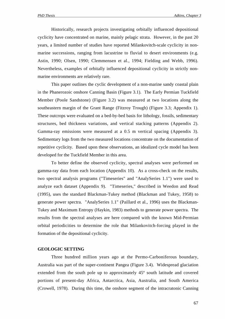
PhD Thesis Adkins, Chapter 3
67
Historically, research projects investigating orbitally influenced depositional
cyclicity have concentrated on marine, mainly pelagic strata. However, in the past 20
years, a limited number of studies have reported Milankovitch-scale cyclicity in non-
marine successions, ranging from lacustrine to fluvial to desert environments (e.g.
Astin, 1990; Olsen, 1990; Clemmensen et al., 1994; Fielding and Webb, 1996).
Nevertheless, examples of orbitally influenced depositional cyclicity in strictly non-
marine environments are relatively rare.
This paper outlines the cyclic development of a non-marine sandy coastal plain
in the Phanerozoic onshore Canning Basin (Figure 3.1). The Early Permian Tuckfield
Member (Poole Sandstone) (Figure 3.2) was measured at two locations along the
southeastern margin of the Grant Range (Fitzroy Trough) (Figure 3.3; Appendix 1).
These outcrops were evaluated on a bed-by-bed basis for lithology, fossils, sedimentary
structures, bed thickness variations, and vertical stacking patterns (Appendix 2).
Gamma-ray emissions were measured at a 0.5 m vertical spacing (Appendix 3).
Sedimentary logs from the two measured locations concentrate on the documentation of
repetitive cyclicity. Based upon these observations, an idealized cycle model has been
developed for the Tuckfield Member in this area.
To better define the observed cyclicity, spectral analyses were performed on
gamma-ray data from each location (Appendix 10). As a cross-check on the results,
two spectral analysis programs ("Timeseries" and "AnalySeries 1.1") were used to
analyze each dataset (Appendix 9). "Timeseries," described in Weedon and Read
(1995), uses the standard Blackman-Tukey method (Blackman and Tukey, 1958) to
generate power spectra. "AnalySeries 1.1" (Paillard et al., 1996) uses the Blackman-
Tukey and Maximum Entropy (Haykin, 1983) methods to generate power spectra. The
results from the spectral analyses are here compared with the known Mid-Permian
orbital periodicities to determine the role that Milankovitch-forcing played in the
formation of the depositional cyclicity.
GEOLOGIC SETTING
Three hundred million years ago at the Permo-Carboniferous boundary,
Australia was part of the super-continent Pangea (Figure 3.4). Widespread glaciation
extended from the south pole up to approximately 45º south latitude and covered
portions of present-day Africa, Antarctica, Asia, Australia, and South America
(Crowell, 1978). During this time, the onshore segment of the intracratonic Canning
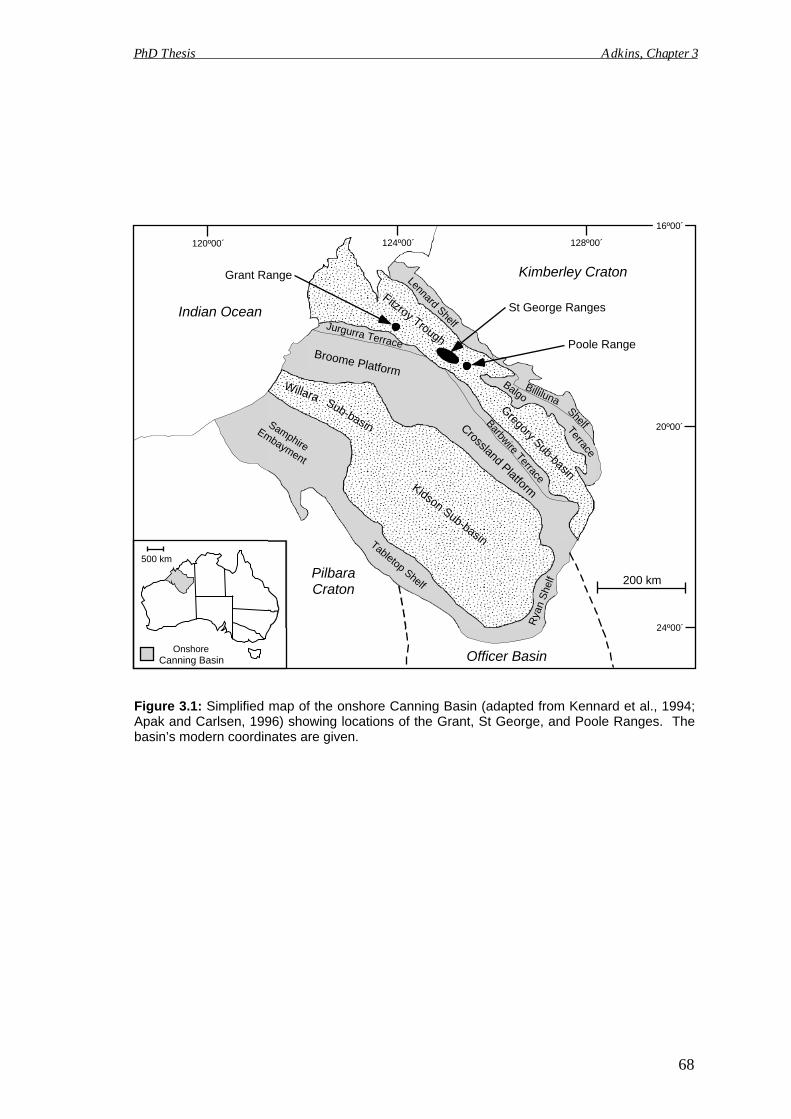
200 km
Onshore
500 km
Willara
Indian Ocean
Kimberley Craton
PilbaraCraton
Officer Basin
Poole Range
St George Ranges
24º00´
20º00´
16º00´
128º00´124º00´120º00´
Fitzroy Trough
Lennard Shelf
BillilunaShelfTerrace
BalgoGregory Sub-basin
Crossland Platform
Broome Platform
Jurgurra Terrace
Barbwire Terrace
Tabletop Shelf
Rya
n S
helf
SamphireEmbayment
Kidson Sub-basin
Sub-basin
Grant Range
Figure 3.1: Simplified map of the onshore Canning Basin (adapted from Kennard et al., 1994;Apak and Carlsen, 1996) showing locations of the Grant, St George, and Poole Ranges. Thebasin’s modern coordinates are given.
PhD Thesis Adkins, Chapter 3
Canning Basin
68
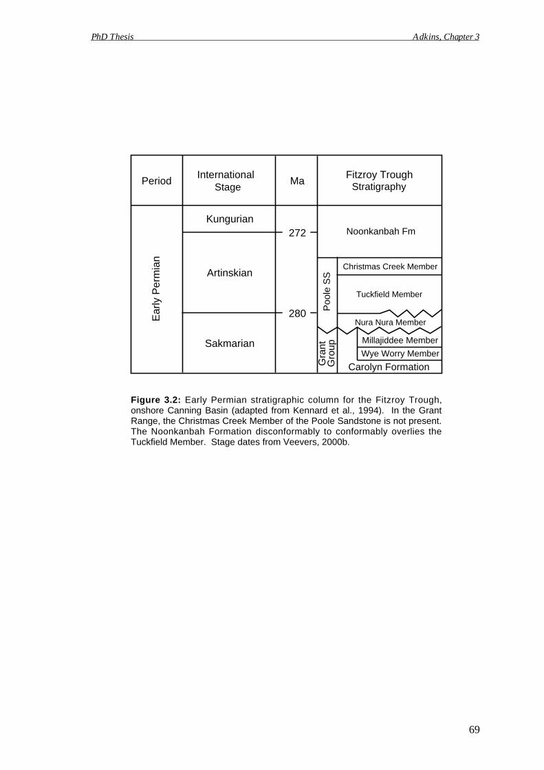
272
280
Fitzroy Trough
Noonkanbah Fm
Poo
le S
S
Christmas Creek Member
Nura Nura Member
Tuckfield Member
Kungurian
Artinskian
Sakmarian
InternationalMaPeriod
Ear
ly P
erm
ian
Carolyn Formation
Millajiddee Member
Wye Worry Member
Gra
ntG
roup
Figure 3.2: Early Permian stratigraphic column for the Fitzroy Trough,onshore Canning Basin (adapted from Kennard et al., 1994). In the GrantRange, the Christmas Creek Member of the Poole Sandstone is not present.The Noonkanbah Formation disconformably to conformably overlies theTuckfield Member. Stage dates from Veevers, 2000b.
PhD Thesis Adkins, Chapter 3
69
Stage Stratigraphy
10 kmNoonkanbah FormationPoole Sandstone Measured Section
FaultGrant AnticlineQuaternary Sediments
Grant Group
Key
G-1
G-2
124º00´
18º00´
124º10´
Figure 3.3: Simplified geological map of the Grant Range (adapted from Crowe and Towner,1981) showing the location of the measured sections.
PhD Thesis Adkins, Chapter 3
70
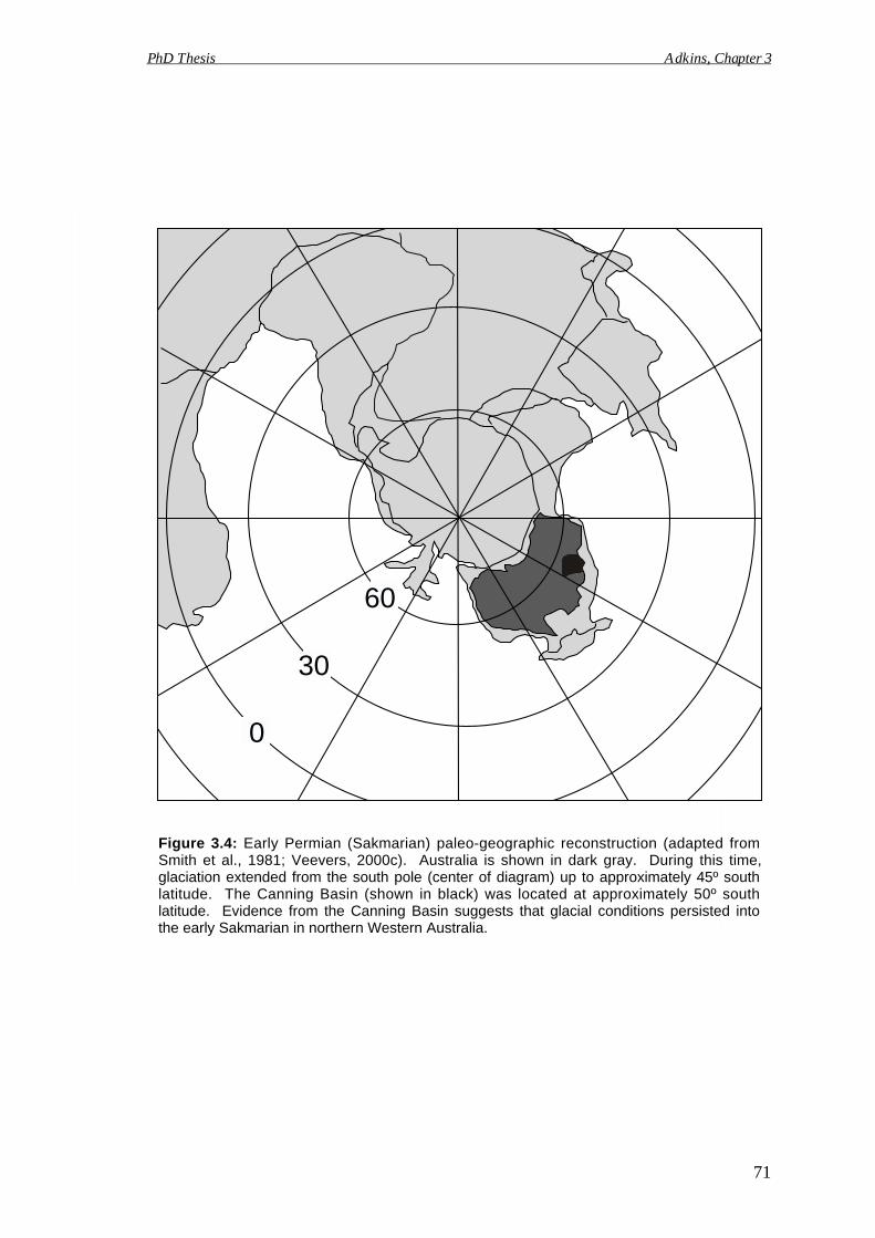
30
0
60
Figure 3.4: Early Permian (Sakmarian) paleo-geographic reconstruction (adapted fromSmith et al., 1981; Veevers, 2000c). Australia is shown in dark gray. During this time,glaciation extended from the south pole (center of diagram) up to approximately 45º southlatitude. The Canning Basin (shown in black) was located at approximately 50º southlatitude. Evidence from the Canning Basin suggests that glacial conditions persisted intothe early Sakmarian in northern Western Australia.
PhD Thesis Adkins, Chapter 3
71
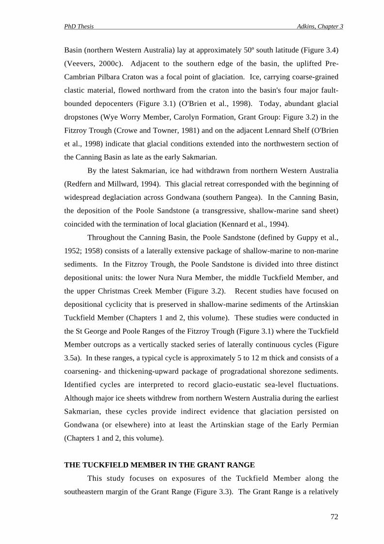
PhD Thesis Adkins, Chapter 3
72
Basin (northern Western Australia) lay at approximately 50º south latitude (Figure 3.4)
(Veevers, 2000c). Adjacent to the southern edge of the basin, the uplifted Pre-
Cambrian Pilbara Craton was a focal point of glaciation. Ice, carrying coarse-grained
clastic material, flowed northward from the craton into the basin's four major fault-
bounded depocenters (Figure 3.1) (O'Brien et al., 1998). Today, abundant glacial
dropstones (Wye Worry Member, Carolyn Formation, Grant Group: Figure 3.2) in the
Fitzroy Trough (Crowe and Towner, 1981) and on the adjacent Lennard Shelf (O'Brien
et al., 1998) indicate that glacial conditions extended into the northwestern section of
the Canning Basin as late as the early Sakmarian.
By the latest Sakmarian, ice had withdrawn from northern Western Australia
(Redfern and Millward, 1994). This glacial retreat corresponded with the beginning of
widespread deglaciation across Gondwana (southern Pangea). In the Canning Basin,
the deposition of the Poole Sandstone (a transgressive, shallow-marine sand sheet)
coincided with the termination of local glaciation (Kennard et al., 1994).
Throughout the Canning Basin, the Poole Sandstone (defined by Guppy et al.,
1952; 1958) consists of a laterally extensive package of shallow-marine to non-marine
sediments. In the Fitzroy Trough, the Poole Sandstone is divided into three distinct
depositional units: the lower Nura Nura Member, the middle Tuckfield Member, and
the upper Christmas Creek Member (Figure 3.2). Recent studies have focused on
depositional cyclicity that is preserved in shallow-marine sediments of the Artinskian
Tuckfield Member (Chapters 1 and 2, this volume). These studies were conducted in
the St George and Poole Ranges of the Fitzroy Trough (Figure 3.1) where the Tuckfield
Member outcrops as a vertically stacked series of laterally continuous cycles (Figure
3.5a). In these ranges, a typical cycle is approximately 5 to 12 m thick and consists of a
coarsening- and thickening-upward package of progradational shorezone sediments.
Identified cycles are interpreted to record glacio-eustatic sea-level fluctuations.
Although major ice sheets withdrew from northern Western Australia during the earliest
Sakmarian, these cycles provide indirect evidence that glaciation persisted on
Gondwana (or elsewhere) into at least the Artinskian stage of the Early Permian
(Chapters 1 and 2, this volume).
THE TUCKFIELD MEMBER IN THE GRANT RANGE
This study focuses on exposures of the Tuckfield Member along the
southeastern margin of the Grant Range (Figure 3.3). The Grant Range is a relatively
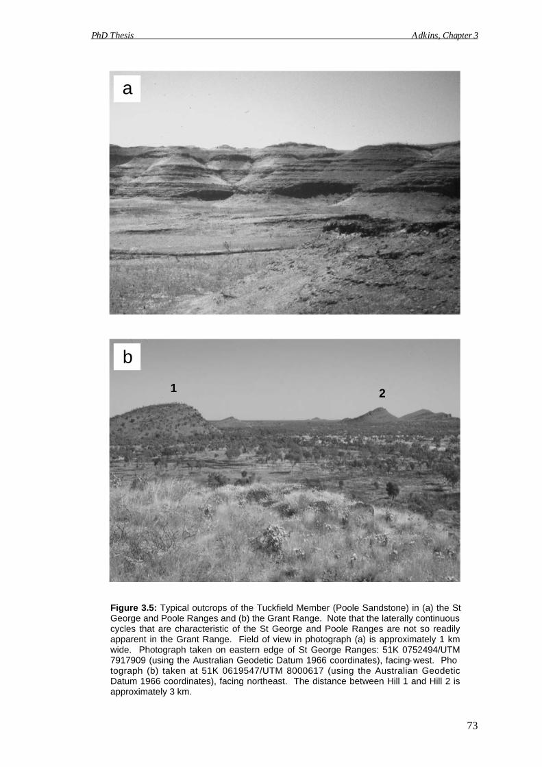
1 2
Figure 3.5: Typical outcrops of the Tuckfield Member (Poole Sandstone) in (a) the StGeorge and Poole Ranges and (b) the Grant Range. Note that the laterally continuouscycles that are characteristic of the St George and Poole Ranges are not so readilyapparent in the Grant Range. Field of view in photograph (a) is approximately 1 kmwide. Photograph taken on eastern edge of St George Ranges: 51K 0752494/UTM7917909 (using the Australian Geodetic Datum 1966 coordinates), facing west. Pho-tograph (b) taken at 51K 0619547/UTM 8000617 (using the Australian GeodeticDatum 1966 coordinates), facing northeast. The distance between Hill 1 and Hill 2 isapproximately 3 km.
a
b
PhD Thesis Adkins, Chapter 3
73

PhD Thesis Adkins, Chapter 3
74
small (approximately 300 km2) anticlinal feature that is located approximately 100 km
northwest of the St George Ranges (Figure 3.1). In the Grant Range, the Tuckfield
Member outcrops as a series of small (typically less than 50 m high), disconnected hills
(Figure 3.5b). Upon first inspection, these deposits appear cyclic and are reminiscent of
the shallow-marine sedimentary cycles observed in the St George and Poole Ranges
(Chapters 1 and 2, this volume). Deposits from all three ranges outcrop as alternating,
cyclic bands of more resistant and less resistant (often unexposed) rock.
However, closer study reveals that Tuckfield Member deposits in the two areas
(Grant Range and St George/Poole Ranges) are inherently different. Although locally
continuous, Grant Range cycles have a limited lateral extent (usually less than 100 m)
and typically cannot be traced from outcrop (hill) to outcrop (hill). In the Grant Range,
the Tuckfield Member (i) is more ferruginous; (ii) is not fossiliferous (no marine trace
or body fossils observed); and (iii) contains more sandstone clasts and individual mud
pellets than in the St George and Poole Ranges.
Two outcrop sections from the Grant Range were measured in detail
(Appendices 2 and 3). The sedimentary log and associated gamma-ray data from
Location G-1 are presented in Figure 3.6. In this representative log, the cyclic
alternation between areas of exposure and non-exposure is evident. Due to superficial
similarities, it would be easy to assume that these cyclic deposits conform to the
coarsening- and thickening-upward cycle model developed for the shallow-marine
sediments of the St George and Poole Ranges (Figure 3.7a). However, a fining- and
thinning-upward cycle model is not only a reasonable alternative but also typically a
more appropriate one (Figure 3.7b). In Figure 3.6a, heavy horizontal lines mark the
boundaries between successive fining- and thinning-upward cycles. At the outcrop
scale, a typical cycle ranges between 2 and 8 m thick.
Cycle Model
In the Grant Range, most Tuckfield Member cycles follow a similar progression
of sediment facies. Because these deposits outcrop as a vertically stacked series of
cycles, a generalized cycle model can be used to describe the basic sedimentology of
the Tuckfield Member in this area (Figure 3.7b).
At its base, a typical cycle consists of medium- to thick-bedded, fine- to
medium-grained sandstone. These sands usually contain large-scale, trough to planar
cross-beds and have erosive bases. Internal laminae (parallel to bedding) and
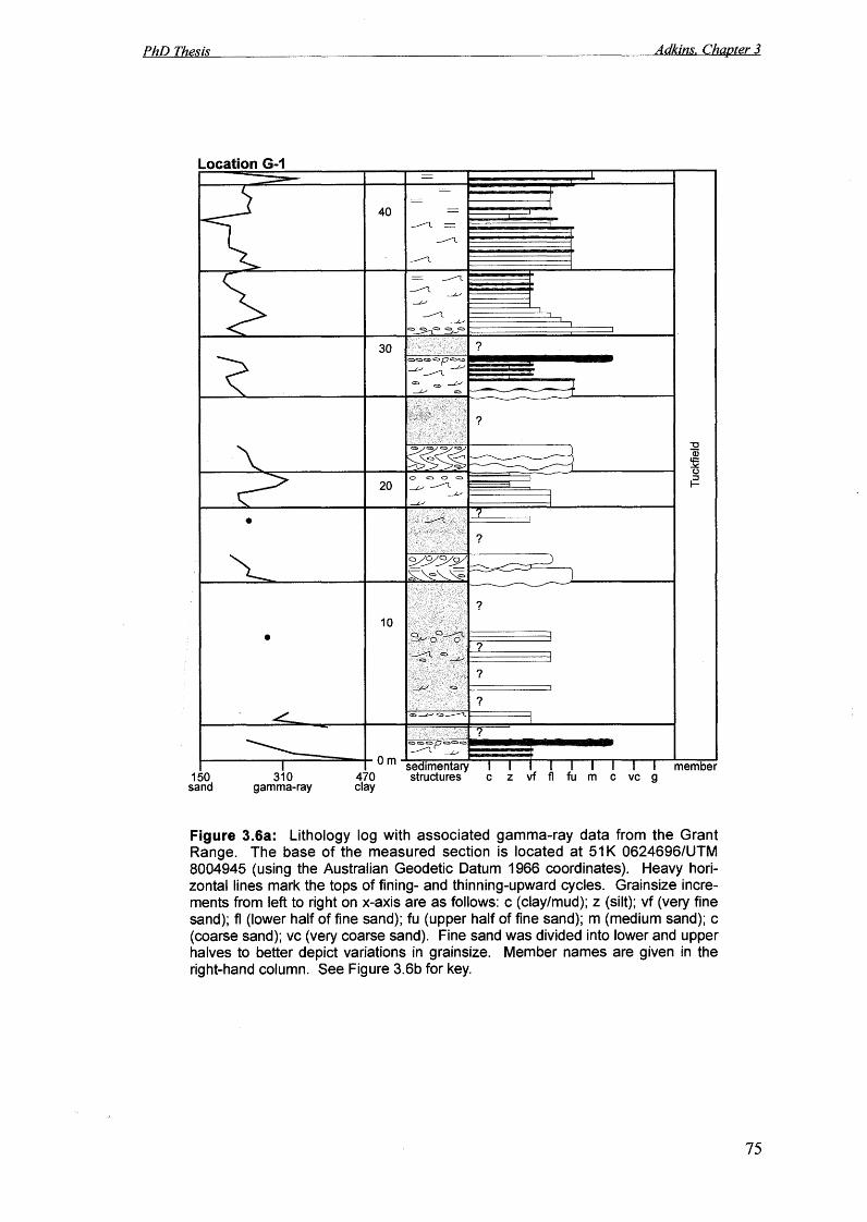
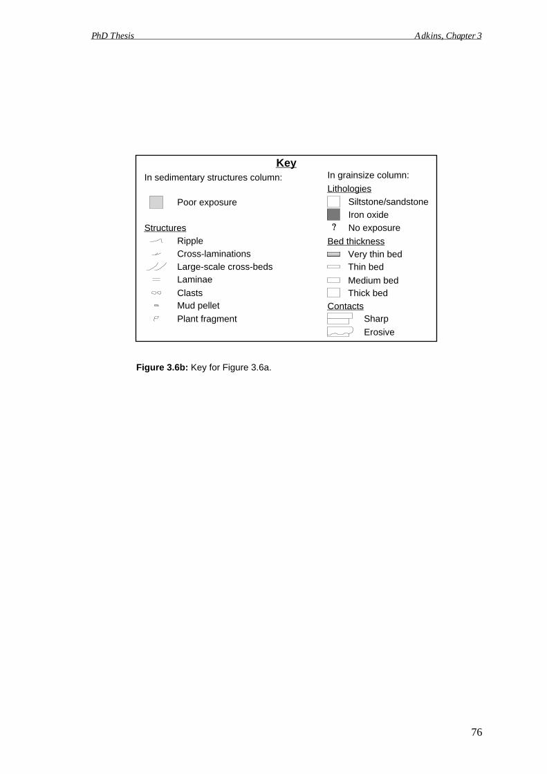
Ripple
Cross-laminations
Laminae
Plant fragment
ClastsMud pellet
Large-scale cross-beds
Structures
Poor exposure
In sedimentary structures column:
Iron oxide
No exposure
Thin bedVery thin bed
Contacts
Thick bed
Erosive
Sharp
Bed thickness
Lithologies
Siltstone/sandstone
In grainsize column:
Medium bed
Key
Figure 3.6b: Key for Figure 3.6a.
PhD Thesis Adkins, Chapter 3
76
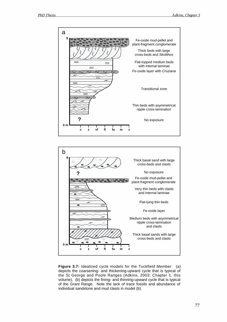
c z vf fl fu m c
0 m
8
? No exposure
Medium beds with asymmetricalripple cross-lamination
and clasts
Very thin beds with clastsand internal laminae
Thick basal sand with largecross-beds and clasts
Fe-oxide mud-pellet andplant-fragment conglomerate
Thick basal sands with largecross-beds and clasts
Fe-oxide layer
Flat-lying thin beds
Figure 3.7: Idealized cycle models for the Tuckfield Member. (a)depicts the coarsening- and thickening-upward cycle that is typical ofthe St George and Poole Ranges (Adkins, 2003; Chapter 1, thisvolume). (b) depicts the fining- and thinning-upward cycle that is typicalof the Grant Range. Note the lack of trace fossils and abundance ofindividual sandstone and mud clasts in model (b).
c z vf fl fu m c
0 m
8
? No exposure
Thin beds with asymmetricalripple cross-lamination
Fe-oxide layer with Cruziana
Flat-topped medium bedswith internal laminae
Transitional zone
Thick beds with largecross-beds and Skolithos
Fe-oxide mud-pellet andplant-fragment conglomerate
a
b
PhD Thesis Adkins, Chapter 3
77
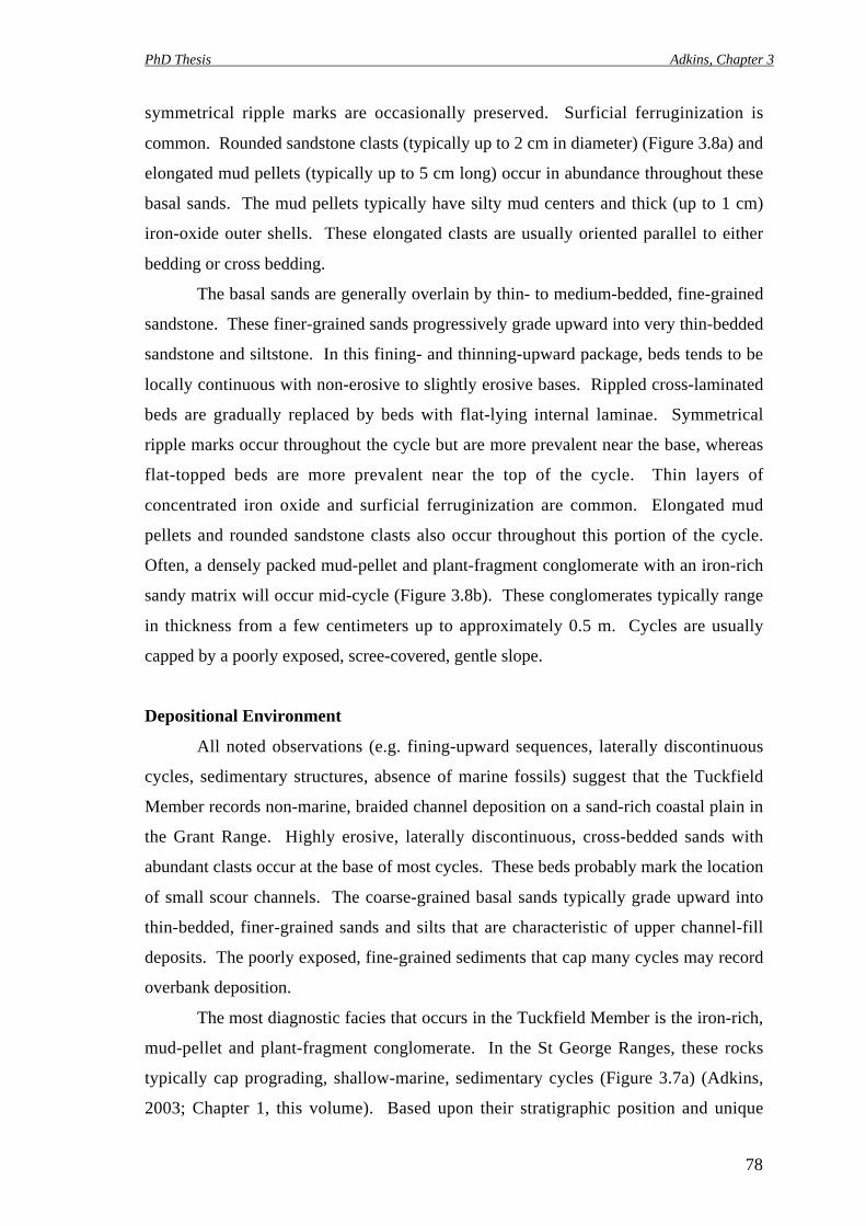
PhD Thesis Adkins, Chapter 3
78
symmetrical ripple marks are occasionally preserved. Surficial ferruginization is
common. Rounded sandstone clasts (typically up to 2 cm in diameter) (Figure 3.8a) and
elongated mud pellets (typically up to 5 cm long) occur in abundance throughout these
basal sands. The mud pellets typically have silty mud centers and thick (up to 1 cm)
iron-oxide outer shells. These elongated clasts are usually oriented parallel to either
bedding or cross bedding.
The basal sands are generally overlain by thin- to medium-bedded, fine-grained
sandstone. These finer-grained sands progressively grade upward into very thin-bedded
sandstone and siltstone. In this fining- and thinning-upward package, beds tends to be
locally continuous with non-erosive to slightly erosive bases. Rippled cross-laminated
beds are gradually replaced by beds with flat-lying internal laminae. Symmetrical
ripple marks occur throughout the cycle but are more prevalent near the base, whereas
flat-topped beds are more prevalent near the top of the cycle. Thin layers of
concentrated iron oxide and surficial ferruginization are common. Elongated mud
pellets and rounded sandstone clasts also occur throughout this portion of the cycle.
Often, a densely packed mud-pellet and plant-fragment conglomerate with an iron-rich
sandy matrix will occur mid-cycle (Figure 3.8b). These conglomerates typically range
in thickness from a few centimeters up to approximately 0.5 m. Cycles are usually
capped by a poorly exposed, scree-covered, gentle slope.
Depositional Environment
All noted observations (e.g. fining-upward sequences, laterally discontinuous
cycles, sedimentary structures, absence of marine fossils) suggest that the Tuckfield
Member records non-marine, braided channel deposition on a sand-rich coastal plain in
the Grant Range. Highly erosive, laterally discontinuous, cross-bedded sands with
abundant clasts occur at the base of most cycles. These beds probably mark the location
of small scour channels. The coarse-grained basal sands typically grade upward into
thin-bedded, finer-grained sands and silts that are characteristic of upper channel-fill
deposits. The poorly exposed, fine-grained sediments that cap many cycles may record
overbank deposition.
The most diagnostic facies that occurs in the Tuckfield Member is the iron-rich,
mud-pellet and plant-fragment conglomerate. In the St George Ranges, these rocks
typically cap prograding, shallow-marine, sedimentary cycles (Figure 3.7a) (Adkins,
2003; Chapter 1, this volume). Based upon their stratigraphic position and unique
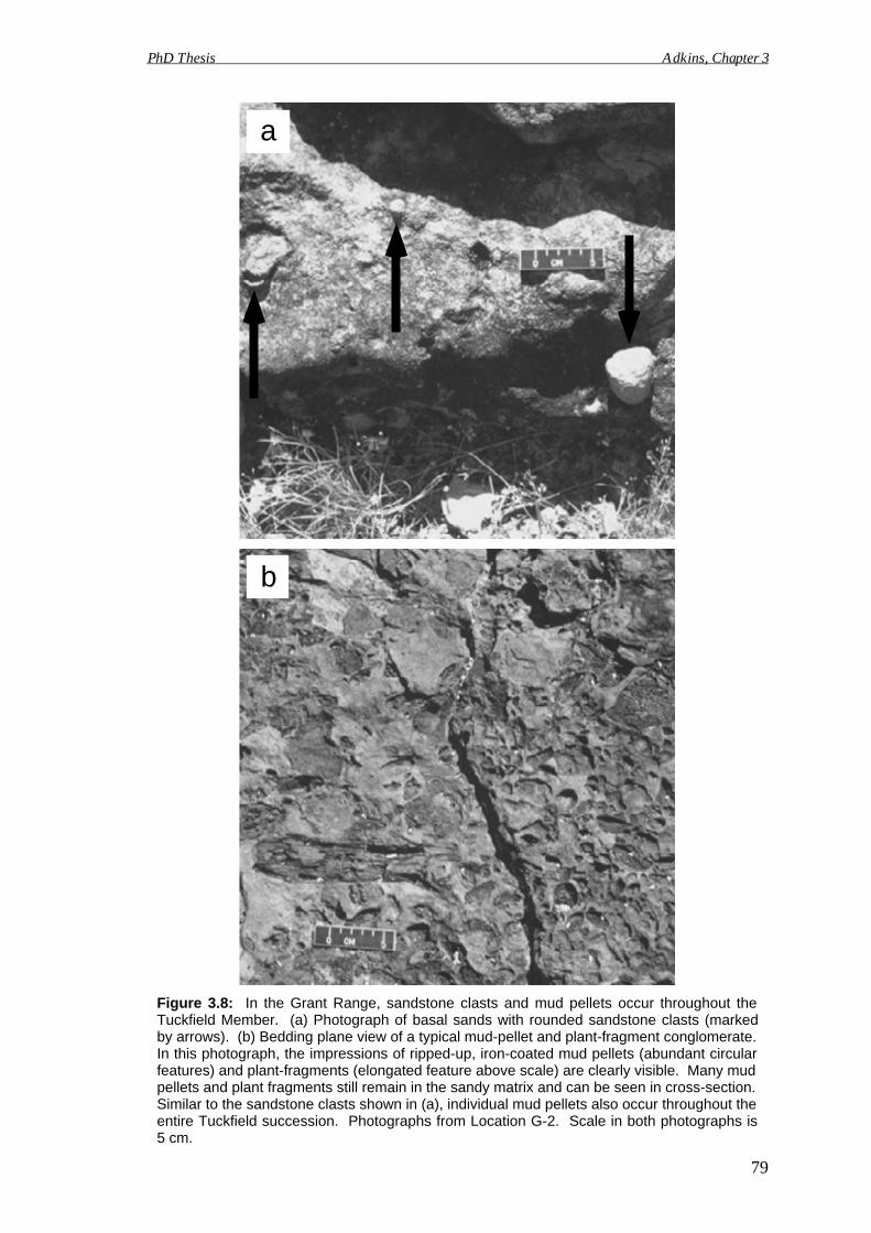
a
b
Figure 3.8: In the Grant Range, sandstone clasts and mud pellets occur throughout theTuckfield Member. (a) Photograph of basal sands with rounded sandstone clasts (markedby arrows). (b) Bedding plane view of a typical mud-pellet and plant-fragment conglomerate.In this photograph, the impressions of ripped-up, iron-coated mud pellets (abundant circularfeatures) and plant-fragments (elongated feature above scale) are clearly visible. Many mudpellets and plant fragments still remain in the sandy matrix and can be seen in cross-section.Similar to the sandstone clasts shown in (a), individual mud pellets also occur throughout theentire Tuckfield succession. Photographs from Location G-2. Scale in both photographs is5 cm.
PhD Thesis Adkins, Chapter 3
79
PhD Thesis Adkins, Chapter 3
80
sedimentary features (fine-grained sediment, abundant plant fragments, iron-rich
nature), Adkins (2003; Chapter 1, this volume) interpreted these conglomerates to be
supratidal/overbank mudflat deposits. If this interpretation is correct, the abundance of
mud pellets (both individual and in conglomerates) in the Grant Range succession again
indicates that the entire sequence was probably deposited in a non-marine, coastal plain
environment.
Today, Tuckfield Member deposits in the Grant Range are dominated by
relatively coarse-grained sediment (very fine to medium-grained sand). However, the
number of silty mud pellets that occur throughout this succession suggest that finer-
grained silts and muds must have been deposited in a nearby area, probably in an
overbank setting. In the St George and Poole Ranges, the shallow-marine sediments of
the Tuckfield Member outcrop as laterally continuous beds. The lateral continuity of
these deposits is generally only interrupted by widespread areal faulting (Figure 3.5a).
In contrast, the non-marine sediments of the Grant Range outcrop as isolated hills that
are separated by distances of 1 to 3 km (Figures 3.3 and 3.5b). The occurrence of these
outcrops appears to be unrelated to faulting (Figure 3.3). Therefore, it is possible that
some of the areas of apparent non-deposition (between outcrops/hills) in the Grant
Range actually mark the locations of previous overbank mudflats. Post-uplift erosion
may have removed these less resistant deposits, leaving sediments that were
predominantly associated with and trapped between the more resistant channel sands.
SPECTRAL ANALYSIS
To better define the depositional cyclicity recorded in the Grant Range, spectral
analyses were performed on the gamma-ray dataset from each location (Appendix 10).**
The results from these analyses are presented in Figures 3.9 (Location G-1) and 3.10
(Location G-2). In both figures, the upper plots (Figures 3.9a and 3.10a) were
generated by the "Timeseries" program and the lower plots (Figures 3.9b and 3.10b)
were generated by the "AnalySeries 1.1" program. Spectral peaks in all four diagrams
(Figures 3.9a, 3.9b, 3.10a and 3.10b) represent cycles recorded in the rock record. The
reciprocal of the frequency for each peak is equal to the average period of that cycle in
** Spectral analyses were also performed on grainsize data from Locations G-1 and G-2 (Appendices 8and 11). Although these analyses do support the conclusions of Chapter 3, the spectral plots are generallynot as well-developed as the plots generated from the analyses of gamma-ray data. Therefore, they arenot discussed in this chapter. However, they are available for consideration in Appendix 11.
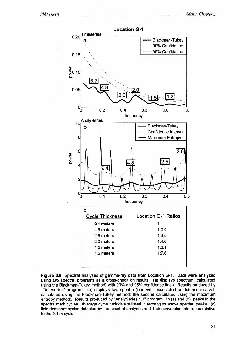
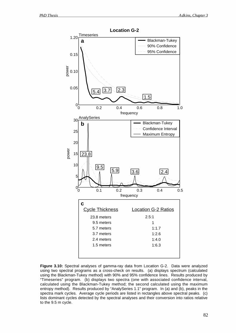
c
Figure 3.10: Spectral analyses of gamma-ray data from Location G-2. Data were analyzedusing two spectral programs as a cross-check on results. (a) displays spectrum (calculatedusing the Blackman-Tukey method) with 90% and 95% confidence lines. Results produced by“Timeseries” program. (b) displays two spectra (one with associated confidence interval,calculated using the Blackman-Tukey method; the second calculated using the maximumentropy method). Results produced by “AnalySeries 1.1" program. In (a) and (b), peaks in thespectra mark cycles. Average cycle periods are listed in rectangles above spectral peaks. (c)lists dominant cycles detected by the spectral analyses and their conversion into ratios relativeto the 9.5 m cycle.
Location G-2
b
0.50.40.30.20.100
5
10
15
20
25
30Blackman-Tukey
Confidence Interval
frequency
pow
er
AnalySeries
23.8
5.9 3.6 2.4
Maximum Entropy
9.5
0 0.2 0.4 0.6 0.8 1.00
0.05
0.10
0.15
1.20Blackman-Tukey90% Confidence
95% Confidence
frequency
pow
er
Timeseries
5.4 3.7 2.3
1.5
Cycle Thickness
23.8 meters
5.7 meters
1.5 meters
2.4 meters
3.7 meters
9.5 meters
Location G-2 Ratios
2.5:1
11:1.7
1:2.6
1:4.0
1:6.3
a
PhD Thesis Adkins, Chapter 3
82
PhD Thesis Adkins, Chapter 3
83
meters (shown in rectangles above spectral peaks). For each location, the spectral peaks
generated by the two programs were compared, averaged, and used to determine the
periodicities of all significant cycles recorded at that location (Figures 3.9c and 3.10c).
According to these analyses, cycles with average periodicities of 9.1 m, 4.6 m, 2.6 m,
2.0 m, 1.5 m and 1.2 m were detected at Location G-1 (Figure 3.9c). Cycles with
average periodicities of 23.8 m, 9.5 m, 5.7 m, 3.7 m, 2.4 m and 1.5 m were detected at
Location G-2 (Figure 3.10c).
MILANKOVITCH CYCLICITY
Rhythmic changes in Earth's orbital path can influence the formation of
depositional cyclicity. Although orbitally influenced cycles are typically associated
with marine strata, recent studies have demonstrated that Milankovitch-scale cyclicity
can also be recorded in non-marine successions (Olsen, 1986; Olsen, 1994; Olsen and
Kent, 1999). Many of these studies have attributed the formation of non-marine cycles
to orbitally-controlled (i) changes in precipitation (Olsen, 1994); (ii) large-scale climatic
variations (e.g. arid versus humid) (Clemmensen et al., 1994); and/or (iii) seasonal
fluctuations in sediment supply (Fielding and Webb, 1996). Additionally, it has long
been postulated that sea-level fluctuations (including glacio-eustatic) can alter baselevel
and thereby influence cyclothem development in fluvial and other non-marine
environments (e.g. Allen, 1964). For these reasons, it is prudent to consider
Milankovitch-forcing as a potential driving mechanism in the formation of any highly
cyclic non-marine succession.
To test for orbital cyclicity in the Tuckfield Member (Grant Range), the
identified cycles (Figures 3. 9 and 3.10) are here compared with the known astronomic
rhythms. The orbital parameters are well established for the present-day with
periodicities of approximately 410,000 years (elongated eccentricity), 100,000 years
(eccentricity), 41,000 years (obliquity), and 19,000 to 23,000 years (precession)
(Berger, 1988; DeBoer and Smith, 1994). However, due to long-term alterations in the
Earth-Moon-Sun rotational system, the values for obliquity and precession have slowly
changed throughout geologic time. During the mid-Permian, obliquity is retrodicted to
have had a periodicity with dual components of 44,000 and 35,000 years. Precession is
retrodicted to have had a periodicity with dual components of 21,000 and 17,600 years.
The periodicities for eccentricity (100,000 years) and elongated eccentricity (410,000
years) have remained relatively constant (Berger and Loutre, 1994).
PhD Thesis Adkins, Chapter 3
84
To effectively compare the identified Tuckfield Member cycles (Figures 3.9 and
3.10) with the mid-Permian orbital periodicities, each set of numbers (e.g. all cycles
identified at Location G-1) must first be converted into a set of ratios. For Location G-
1, this conversion is shown in Figure 3.9c. For example, if the 9.1 m cycle is set at one,
the number of 4.6 m cycles in each 9.1 m cycle is 2.0 (9.1 ÷ 4.6 = 2.0). For Location G-
2, a similar conversion is shown in Figure 3.10c. The mid-Permian orbital periodicities
were converted into ratios by setting the 100,000 year cycle equal to one. For example,
the number of 44,000 year cycles in each 100,000 year cycle is equal to 2.3 (100,000 ÷
44,000 = 2.3). The complete listing of the mid-Permian Milankovitch ratios is given in
the second line of Table 3.1.
In addition to listing the mid-Permian orbital periodicities and their associated
ratios, Table 3.1 also lists the ratios from Locations G-1 and G-2 (originally given in
Figures 3.9c and 3.10c) and the average cycle periodicities detected in deposits from the
St George and Poole Ranges (from the analyses of gamma-ray data: Chapter 2, this
volume). Clearly, the non-marine cycles identified in the Grant Range (Locations G-1
and G-2) compare favorably with the orbital periodicities and with the shallow-marine
cycles detected in the other areas. Extra, non-Milankovitch-band cycles (in unmarked
columns) detected in the St George and Poole Ranges have been interpreted to be the
result of tectonic events or short-term changes in sediment supply (Chapter 2, this
volume). The extra cycle detected at Location G-1 (1:7.6) may also record tectonism or
short-term changes in sediment supply. However, it is equally possible that this cycle is
merely a spurious peak in the spectral plot.
It should also be noted that the shallow-marine, Milankovitch-band cyclicity
recorded in the St George and Poole Ranges appears to conform more closely to the
expected Milankovitch periodicities than do the non-marine cycles recorded in the
Grant Range. Although this may be a true representation, it is probable that this is
simply a result of sampling. The values listed for the St George and Poole Ranges
(Table 3.1) are averaged from 15 measured sections. The values listed under Locations
G-1 and G-2 (Table 3.1) each represent one measured section. Obviously, the more
samples that are averaged together, the more accurate the results will be.
DEPOSITIONAL MODEL FOR THE FITZROY TROUGH
During the Artinskian when the Tuckfield Member was deposited, the Fitzroy
Trough was comprised of a complex system of shallow-marine to non-marine
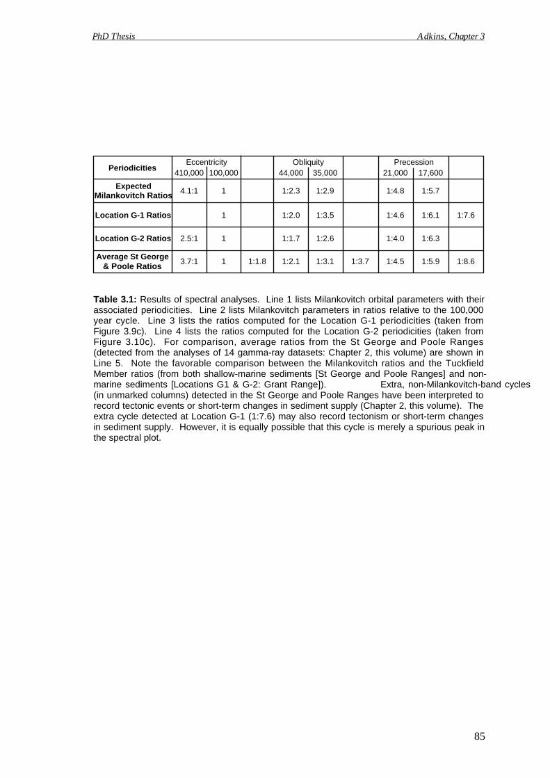
Expected
Location G-1 Ratios
Obliquity44,000 35,000410,000
Eccentricity100,000
Precession21,000 17,600
4.1:1 1 1:2.3 1:2.9 1:4.8 1:5.7
1:6.11:4.61:3.51:2.01
Periodicities
Location G-2 Ratios 2.5:1 1 1:1.7 1:2.6 1:4.0 1:6.3
Average St George1:5.91:4.51:3.11:2.113.7:1 1:3.71:1.8 1:8.6
1:7.6
Table 3.1: Results of spectral analyses. Line 1 lists Milankovitch orbital parameters with theirassociated periodicities. Line 2 lists Milankovitch parameters in ratios relative to the 100,000year cycle. Line 3 lists the ratios computed for the Location G-1 periodicities (taken fromFigure 3.9c). Line 4 lists the ratios computed for the Location G-2 periodicities (taken fromFigure 3.10c). For comparison, average ratios from the St George and Poole Ranges(detected from the analyses of 14 gamma-ray datasets: Chapter 2, this volume) are shown inLine 5. Note the favorable comparison between the Milankovitch ratios and the TuckfieldMember ratios (from both shallow-marine sediments [St George and Poole Ranges] and non-marine sediments [Locations G1 & G-2: Grant Range]). Extra, non-Milankovitch-band cycles(in unmarked columns) detected in the St George and Poole Ranges have been interpreted torecord tectonic events or short-term changes in sediment supply (Chapter 2, this volume). Theextra cycle detected at Location G-1 (1:7.6) may also record tectonism or short-term changesin sediment supply. However, it is equally possible that this cycle is merely a spurious peak inthe spectral plot.
PhD Thesis Adkins, Chapter 3
85
Milankovitch Ratios
& Poole Ratios
PhD Thesis Adkins, Chapter 3
86
depositional environments (Figure 3.11). In the St George and Poole Ranges, the
Artinskian Tuckfield Member outcrops as a series of shallow-marine cycles. Recent
studies (Chapters 1 and 2, this volume) have directly linked these cycles to Earth's
orbital parameters and attributed the formation of depositional cyclicity to glacio-
eustatic sea-level fluctuation. In the nearby Grant Range, the Tuckfield Member
outcrops as a series of non-marine cycles. This study demonstrates a favorable
comparison between these non-marine cycles and the known mid-Permian orbital
periodicities. This favorable comparison indicates that Milankovitch-forcing of climate
influenced the formation of non-marine cyclicity in the Grant Range.
As previously mentioned, Earth's orbital perturbations can affect global sea-
level. Additionally, orbital cyclicity can influence precipitation, large-scale climatic
variations, and seasonal fluctuations in sediment supply. Therefore, it could be difficult
to determine the exact mechanism of formation for many non-marine cyclic
successions. However, the strong correlation between the identified non-marine and
shallow-marine Tuckfield Member cycles (Table 3.1) suggests that the same
mechanism probably controlled the formation of depositional cyclicity in both
environments. Adkins (Chapter 2, this volume) proposed that global sea-level
fluctuation, related to the waxing and waning of Gondwanan glaciers, drove the
deposition of shallow-marine cyclicity in the St George and Poole Ranges. This same
sea-level fluctuation may have affected local base-level in the Fitzroy Trough, thereby
forcing the rhythmic migration of non-marine, coastal plain environments. As these
glacially-driven changes in base-level forced the Grant Range coastal plain to migrate,
local channel-shifting may have resulted in the deposition of the vertically stacked,
fining- and thinning-upward cycles observed in outcrop.
CONCLUSIONS
In the Grant Range, at least eight vertically stacked, fining- and thinning-upward
Tuckfield Member cycles have been identified. Each cycle contains lithologies and
sedimentary structures that are indicative of non-marine, braided channel deposition on
a sand-rich coastal plain. Spectral analysis of gamma-ray data was used to constrain the
depositional cyclicity that is observed in outcrop. Identified cycles correlate strongly
with the known mid-Permian orbital periodicities of eccentricity, obliquity, and
precession. This favorable comparison indicates that Milankovitch-forcing of climate is
responsible for the formation of these cycles. Additionally, the calculated ratios for the
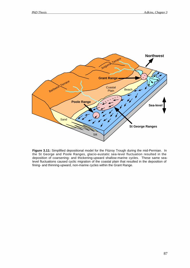
St George Ranges
Poole Range
Grant Range
Sand
Silt
CoastalPlain Beach
Jurgurra Terra
ce
Barbwire Terrace
Sea-level
Northwest
Figure 3.11: Simplified depositional model for the Fitzroy Trough during the mid-Permian. Inthe St George and Poole Ranges, glacio-eustatic sea-level fluctuation resulted in thedeposition of coarsening- and thickening-upward shallow-marine cycles. These same sea-level fluctuations caused cyclic migration of the coastal plain that resulted in the deposition offining- and thinning-upward, non-marine cycles within the Grant Range.
PhD Thesis Adkins, Chapter 3
87

PhD Thesis Adkins, Chapter 3
non-marine cyclicity that was identified in the Grant Range is similar to the correlative
calculated ratios for the shallow-marine cyclicity that was identified in the St George
and Poole Ranges (eccentricity, obliquity, and precession). This suggests that glacio-
eustatic sea-level fluctuations probably controlled both the formation of shallow-marine
and non-marine (coastal plain) cyclicity in the mid-Permian Fitzroy Trough. These
findings act as a reminder that Milankovitch-forcing of climate should never be
dismissed as a potential driving-mechanism in the formation of non-marine depositional
cyclicity.
88

PhD Thesis Adkins, Chapter 4
Chapter 4
The stratigraphic evolution and petroleum potential ofthe Early Permian Poole Sandstone, onshore Canning
Basin, Western Australia
PhD Thesis Adkins, Chapter 4
90
ABSTRACT
The Early Permian Poole Sandstone occurs throughout the northwestern region
of the onshore Canning Basin, Western Australia. Although the Poole Sandstone has
long been identified as a potential petroleum reservoir, its sub-surface stratigraphic
evolution has not been studied in any detail. This investigation focuses on the
sedimentology and stratigraphy of the unit as it occurs in the northern Fitzroy
Trough/Lennard Shelf region. In this area, the Poole Sandstone can be traced
throughout the sub-surface as a continuous package of predominantly shallow-marine
sediments. The two distinct depositional units that together comprise the Poole
Sandstone are easily recognized on sub-surface gamma-ray logs. The lower Nura Nura
Member unconformably overlies the Early Permian Grant Group and probably consists
of a heterogeneous package of predominantly clastic sediments. Its unconformable
nature, combined with the lateral variability of the Nura Nura deposits, makes the lower
bounding surface of the Poole Sandstone difficult to identify in well logs with certainty.
In contrast, the bounding surface between the Nura Nura Member and the overlying
Tuckfield Member is easily recognized, as is the bounding surface between the
Tuckfield Member and the overlying Noonkanbah Formation
Because the Tuckfield Member is well constrained within the study area, it is
possible to perform detailed stratigraphic analyses of this unit. In the northern Fitzroy
Trough/Lennard Shelf region, the Tuckfield Member ranges from 39 to 68 m thick and
consists of a coarsening-upward package of predominantly shallow-marine clastic
sediments. This large-scale coarsening-upward cycle is comprised of four distinct,
smaller-scale coarsening-upward cycles of approximately equal thickness. The
Tuckfield Member and each of its four internal cycles can be traced laterally throughout
the field area for a distance of over 200 km. Parallel to the paleo-coastline, these cycles
maintain a near constant thickness. Oblique to the paleo-coastline, these cycles both
thicken and deepen basinward.
To gain a better understanding of the observed cyclicity, spectral analyses were
performed on gamma-ray data from the Terrace 1 log. These analyses indicate that the
Poole Sandstone probably records a variety of sea-level fluctuations of both orbital and
tectonic origin.
Key Words: Canning Basin, cyclicity, Fitzroy Trough, Permian, Poole Sandstone,
Tuckfield Member
PhD Thesis Adkins, Chapter 4
91
INTRODUCTION
The onshore segment of the Phanerozoic Canning Basin has potential for
significant hydrocarbon production (e.g. Kennard et al., 1994). Lying mainly within the
Great Sandy and Gibson Deserts of Western Australia, the onshore Canning Basin
covers an area larger than Texas (430,000 km2) and has a basin fill of up to 18 km
(Yeates et al., 1984). The sediments that fill the basin were predominantly deposited
from the Early Ordovician to the Early Cretaceous in a shallow-marine environment.
These sediments contain thick reservoir-quality sandstone and carbonate units (Kennard
et al., 1994).
To date, hydrocarbon exploration within the Canning Basin has met with limited
success. However, several small petroleum fields, identified in the basin’s northern
regions (Middleton, 1992; Griffin et al., 1993), suggest that larger hydrocarbon
accumulations may also exist. With fewer than 300 exploration wells scattered
throughout the area (Apak and Carlsen, 1996), parts of the onshore Canning Basin are
relatively untested and the potential for commercial petroleum discovery remains high.
Exploration within the basin has historically focused on its northwestern region.
Since the 1920s, more than 250 petroleum wells have been drilled throughout the
Canning Basin area. Of these, approximately 45% are located in the Fitzroy Trough
(15%) and on the adjacent Lennard Shelf (30%) (Apak and Carlsen, 1996) (Figure 4.1).
In this region, commercial hydrocarbon accumulations have been identified in
terrigenous Permo-Carboniferous strata (e.g. the Early Permian Grant Group) and
carbonate reservoirs from the Devonian reef complex (Griffin et al., 1993; Apak and
Carlsen, 1996). Additionally, a few historically non-productive Permo-Carboniferous
units have been identified as potential petroleum reservoirs (Towner, 1981; Jackson et
al., 1994).
The Early Permian Poole Sandstone (defined by Guppy et al., 1952, 1958) is one
such unit. It has largely been marked as a potential petroleum reservoir based upon
favorable porosity/permeability values and recorded hydrocarbon shows (e.g. Havord et
al., 1997). Although it may be economically important, little is known about the sub-
surface stratigraphic evolution of this unit. To date, few detailed sedimentological
and/or stratigraphic analyses have been performed on the Poole Sandstone. The studies
that do exist concentrate predominantly on high-frequency cyclicity that is recorded in
relatively limited outcrop exposures (Grant, St George, and Poole Ranges: Figure 4.1)
of the middle Tuckfield Member (Adkins, 2003; Chapters 1-3, this volume). To
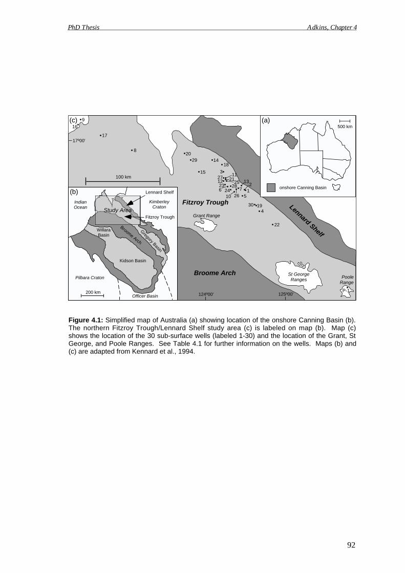
(b)
IndianOcean
KimberleyCraton
Pilbara Craton
Officer Basin
Study Area
Broome Arch
Fitzroy Trough
Gregory Basin
Kidson Basin
WillaraBasin
200 km
500 km
onshore Canning Basin
(a)
St GeorgeRanges Poole
Range
Grant Range
(c)
22
419
16
9
2029 14
18
327
1121
6 2410
7
13
12
5
Lennard Shelf
Fitzroy Trough
Broome Arch
100 km
124º00' 125º00'
17º00'
P-1
26
30
282512
23
15
8
17
PhD Thesis Adkins, Chapter 4
Lennard Shelf
Figure 4.1: Simplified map of Australia (a) showing location of the onshore Canning Basin (b).The northern Fitzroy Trough/Lennard Shelf study area (c) is labeled on map (b). Map (c)shows the location of the 30 sub-surface wells (labeled 1-30) and the location of the Grant, StGeorge, and Poole Ranges. See Table 4.1 for further information on the wells. Maps (b) and(c) are adapted from Kennard et al., 1994.
92
PhD Thesis Adkins, Chapter 4
93
effectively evaluate the hydrocarbon potential of the Poole Sandstone, it is necessary to
first understand its sub-surface stratigraphic evolution. This chapter provides a detailed
analysis of the sub-surface Poole Sandstone (concentrating on the middle Tuckfield
Member) as it occurs in the northwestern region of the onshore Canning Basin (Figure
4.1).
DATABASE AND METHODS
This research focuses on sub-surface data from the northern Fitzroy Trough and
the adjacent Lennard Shelf. Gamma-ray logs, obtained from hydrocarbon exploration
wells, were collected from an area that covers approximately 15,000 km2 and includes
more than 70 petroleum wells (Figure 4.1). The Early Permian Nura Nura and
Tuckfield Members of the Poole Sandstone were identified on each of the 70+ logs. Of
these logs, 30 were chosen for inclusion in this study (Figure 4.1 and Table 4.1). The
chosen logs are of high quality, record complete preservation of the Poole Sandstone
(e.g. no section is faulted out), and provide non-repetitive lateral coverage of the study
area. For example, all of the Sundown wells (1-5) occur within approximately 1 km2.
Therefore, their logs are near replicas of each other. To avoid the use of repetitive data,
only one of these wells (Sundown 2) is included in this investigation.
Based upon the 30 chosen gamma-ray logs, cross-sections and an isopach map
of the Tuckfield Member were constructed. These diagrams are used to establish the
depositional environment and lateral variability of the unit. Additionally, sub-surface
data from this area is compared with outcrop observations taken from the nearby Poole
Range (Figure 4.1). The similarity between the two datasets allows sub-surface
stratigraphic and sedimentological interpretations to be made with confidence.
In the study area, several orders of cyclicity, recognized in the Tuckfield
Member, can be traced laterally for more than 200 km. To define the observed cyclicity
better, spectral analyses were performed on gamma-ray measurements taken at a one-
meter vertical spacing (from a depth of 775 m in the Noonkanbah Formation to a depth
of 950 m in the Grant Group) on the Terrace 1 log (Appendix 12). To verify the results,
this dataset was analyzed using two different spectral analysis programs (Appendix 9).
The “Timeseries” program (described by Weedon and Read, 1995) uses the standard
Blackman-Tukey method (Blackman and Tukey, 1958) to generate power spectra,
whereas the “AnalySeries 1.1” program (Paillard et al., 1996) uses both the Blackman-
Tukey and Maximum Entropy (Haykin, 1983) methods to generate power spectra. The
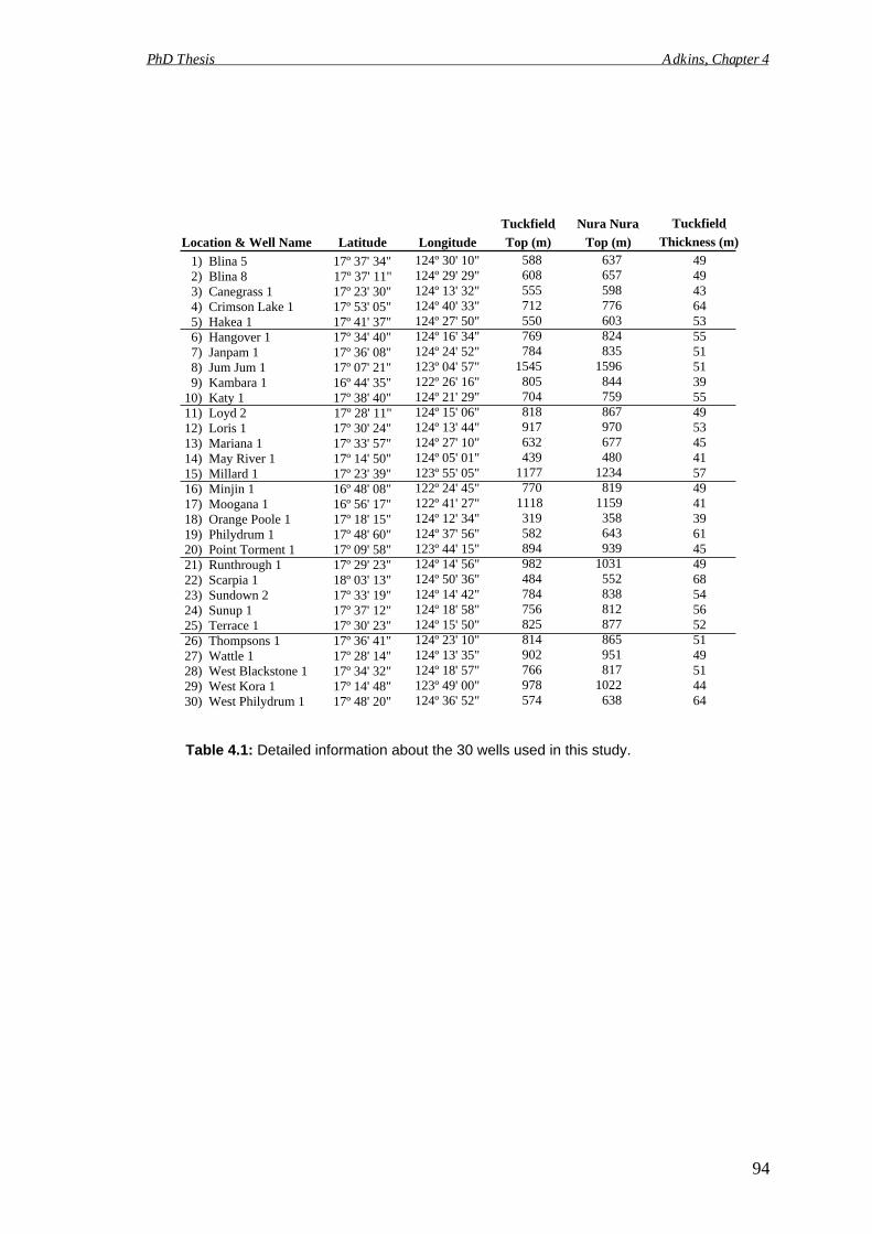
Location & Well Name 1) Blina 5 2) Blina 8 3) Canegrass 1 4) Crimson Lake 1 5) Hakea 1 6) Hangover 1 7) Janpam 1 8) Jum Jum 1 9) Kambara 110) Katy 111) Loyd 212) Loris 113) Mariana 114) May River 115) Millard 116) Minjin 117) Moogana 118) Orange Poole 119) Philydrum 120) Point Torment 121) Runthrough 122) Scarpia 123) Sundown 224) Sunup 125) Terrace 126) Thompsons 127) Wattle 128) West Blackstone 129) West Kora 130) West Philydrum 1
Latitude17º 37' 34"17º 37' 11"17º 23' 30"17º 53' 05"17º 41' 37"17º 34' 40"17º 36' 08"17º 07' 21"16º 44' 35"17º 38' 40"17º 28' 11"17º 30' 24"17º 33' 57"17º 14' 50"17º 23' 39"16º 48' 08"16º 56' 17"17º 18' 15"17º 48' 60"17º 09' 58"17º 29' 23"18º 03' 13"17º 33' 19"17º 37' 12"17º 30' 23"17º 36' 41"17º 28' 14"17º 34' 32"17º 14' 48"17º 48' 20"
Longitude124º 30' 10"124º 29' 29"124º 13' 32"124º 40' 33"124º 27' 50"124º 16' 34"124º 24' 52"123º 04' 57"122º 26' 16"124º 21' 29"124º 15' 06"124º 13' 44"124º 27' 10"124º 05' 01"123º 55' 05"122º 24' 45"122º 41' 27"124º 12' 34"124º 37' 56"123º 44' 15"124º 14' 56"124º 50' 36"124º 14' 42"124º 18' 58"124º 15' 50"124º 23' 10"124º 13' 35"124º 18' 57"123º 49' 00"124º 36' 52"
TuckfieldTop (m)
588608555712550769784
1545805704818917632439
1177770
1118319582894982484784756825814902766978574
Nura NuraTop (m)
637657598776603824835
1596844759867970677480
1234819
1159358643939
1031552838812877865951817
1022638
TuckfieldThickness (m)
494943645355515139554953454157494139614549685456525149514464
PhD Thesis Adkins, Chapter 4
Table 4.1: Detailed information about the 30 wells used in this study.
94
PhD Thesis Adkins, Chapter 4
95
detected cycles are herein compared with cyclicity identified in shallow-marine
Tuckfield Member deposits from the Poole Range (Figure 1.4) (Chapter 2, this volume).
This comparison plays a critical role in determining the significance of the cyclicity
observed in the study area.
Due to poor imaging associated with shallow sub-surface depths and the
relatively thin nature of the Poole Sandstone, seismic data was not used in this study.
GEOLOGIC SETTING
The Fitzroy Trough is a northwest-trending graben bounded by the Beagle Bay
and Pinnacle Fault Systems to the northeast and by the Fenton Fault System to the
southwest (Towner, 1981). Development of both the Fitzroy Trough and the larger
Canning Basin began during the Ordovician when thrust-related shearing in basement
rock to the north (Shaw et al., 1992a) resulted in extension and rapid subsidence of the
Canning Basin area. The Fitzroy Trough contains over 15 km of Paleozoic and minor
Mesozoic sediments that can be divided into four distinct tectono-stratigraphic
megasequences: (i) Ordovician-Silurian; (ii) Devonian-Early Carboniferous; (iii) Late
Carboniferous-Permian; and (iv) Jurassic-Cretaceous. Each of these megasequences
corresponds to a transgressive-regressive package that records an episode of crustal
stretching and subsidence followed by an extended period of tectonic quiescence
(Kennard et al., 1994).
To the northeast, the Beagle Bay and Pinnacle Fault Systems separate the
northern Fitzroy Trough from the adjacent Lennard Shelf. A thin succession (generally
less than 2 km thick) of Paleozoic basin strata overlies shallow basement rock in the
Lennard Shelf area. These strata typically thicken (Towner, 1981) and deepen (from
diagrams in: Towner, 1981; Gibson, 1983; Purcell and Poll, 1984) basinward. They
consist of mainly Devonian reef and reef-associated deposits with lesser accumulations
of Ordovician and Carboniferous-Triassic rocks (Towner, 1981). The major faults that
separate the Fitzroy Trough from the Lennard Shelf are predominantly near-vertical
normal faults that offset sediments in the area by as much as several kilometers (Yeates
et al., 1984). Offset associated with these faults is greatest at depth and lessens higher
in the section (e.g. Towner, 1981; Gibson, 1983). The Early Permian Poole Sandstone
is one of the oldest stratigraphic units that is relatively continuous across the northern
Fitzroy Trough/Lennard Shelf area.

PhD Thesis Adkins, Chapter 4
96
Within the Canning Basin, the Poole Sandstone consists of a laterally extensive
package of shallow-marine and non-marine sediments. Three distinct depositional units
comprise the Poole Sandstone: the lower Nura Nura Member, the middle Tuckfield
Member, and the upper Christmas Creek Member (Crowe and Towner, 1976a).
Although the middle Tuckfield Member occurs throughout the Canning Basin, the
lower Nura Nura Member is restricted to the northwestern region of the basin (Crowe
and Towner, 1977) and the upper Christmas Creek Member has only been identified in
outcrop exposures of the St George and Poole Ranges (Crowe and Towner, 1976a).
OUTCROP CHARACTERISTICS
The best exposures of the Poole Sandstone are found in the Grant, St George,
and Poole Ranges of the Fitzroy Trough (Figure 4.1). Detailed stratigraphic analyses of
the unit (concentrating on the middle Tuckfield Member) were recently conducted in all
three areas (Adkins, 2003; Chapters 1-3, this volume). In these ranges, the Sakmarian
to Artinskian Nura Nura Member unconformably overlies fluvio-marine to deltaic,
near-shore deposits of the upper Grant Group (Figure 4.2) (Apak, 1996). In these
ranges, the Nura Nura Member is less than 30 m thick (Crowe and Towner, 1981) and
consists of a heterogeneous mix of clastic sediments. These sediments record
deposition in a variety of shallow-marine to non-marine environments (Crowe and
Towner, 1976b).
In the Grant, St George, and Poole Ranges, the Artinskian Tuckfield Member
conformably to unconformably overlies the Nura Nura Member (Figure 4.2) (Crowe
and Towner, 1981). The unit ranges in thickness from less than 50 m in the Grant and
Poole Ranges to greater than 100 m in parts of the St George Ranges. In outcrop, this
unit records a variety of depositional environments that range from non-marine coastal
plain settings (Grant Range) to shallow-marine shoreface settings (Poole Range)
(Adkins, 2003; Chapters 1-3, this volume).
In the Poole Range area, the Tuckfield Member outcrops as an approximately 40
m thick package of vertically stacked, coarsening- and thickening-upward cycles
(Figure 4.3). Well-defined natural benches usually correspond with cycle tops and can
be traced laterally throughout the range (Figures 4.3 and 4.4). Individual cycles are
typically 5 to 7 m thick, but some thinner cycles (2 to 4 m) also occur within the
Tuckfield Member succession (Figure 4.3) (Chapter 2, this volume). Each cycle
systematically coarsens upward from silty mudstone to siltstone to sandstone. Primary
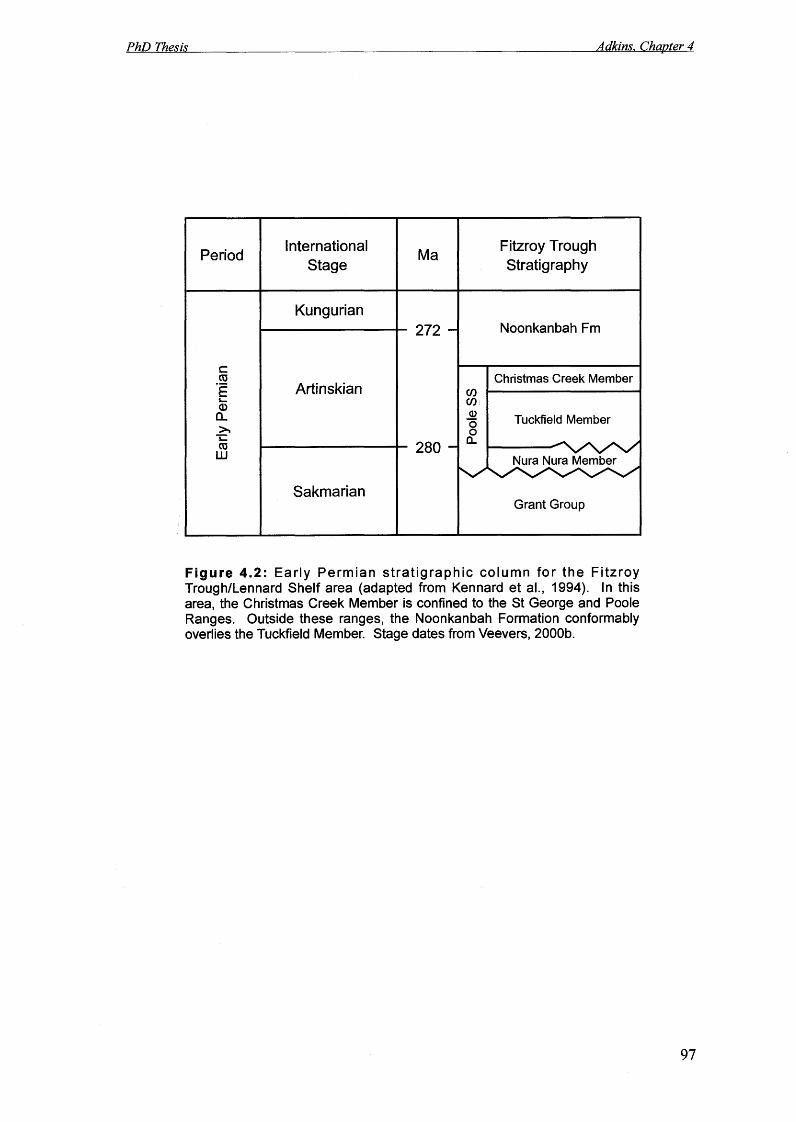
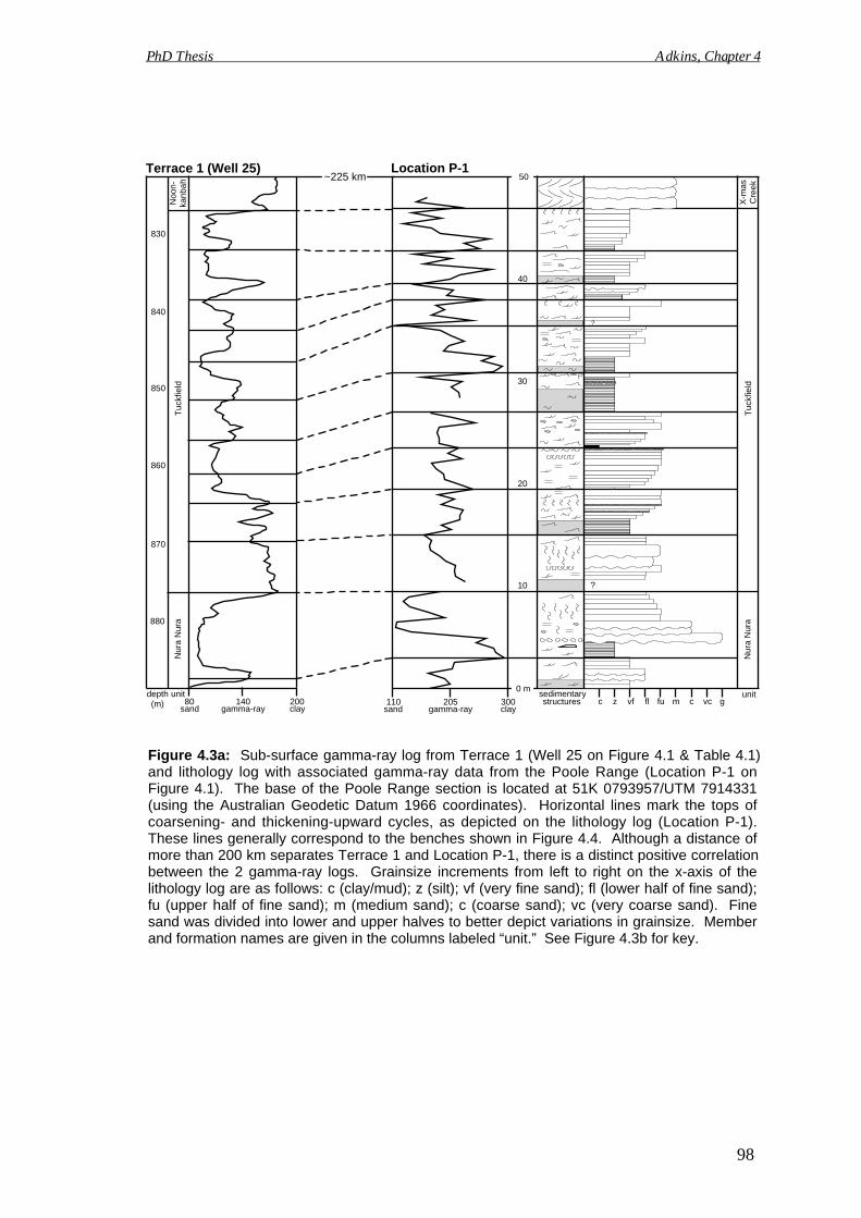
205gamma-ray
110 300 c z vf fl fu m c vc gsand clay
?
?
sedimentarystructures
X-m
asC
reek
Nur
a N
ura
Tuc
kfie
ld
40
30
20
10
Location P-1
0 m
850
140gamma-ray
80 200sand clay
50Terrace 1 (Well 25)
840
830
860
870
880
unit unitdepth(m)
Nur
a N
ura
Tuc
kfie
ldN
oon-
kanb
ah~225 km
PhD Thesis Adkins, Chapter 4
Figure 4.3a: Sub-surface gamma-ray log from Terrace 1 (Well 25 on Figure 4.1 & Table 4.1)and lithology log with associated gamma-ray data from the Poole Range (Location P-1 onFigure 4.1). The base of the Poole Range section is located at 51K 0793957/UTM 7914331(using the Australian Geodetic Datum 1966 coordinates). Horizontal lines mark the tops ofcoarsening- and thickening-upward cycles, as depicted on the lithology log (Location P-1).These lines generally correspond to the benches shown in Figure 4.4. Although a distance ofmore than 200 km separates Terrace 1 and Location P-1, there is a distinct positive correlationbetween the 2 gamma-ray logs. Grainsize increments from left to right on the x-axis of thelithology log are as follows: c (clay/mud); z (silt); vf (very fine sand); fl (lower half of fine sand);fu (upper half of fine sand); m (medium sand); c (coarse sand); vc (very coarse sand). Finesand was divided into lower and upper halves to better depict variations in grainsize. Memberand formation names are given in the columns labeled “unit.” See Figure 4.3b for key.
98

MudstoneRipple
Swaley/hummocky cross-bed Iron oxide
Cross-laminations No exposure
Silt/sand stringer Thin bed
Laminae Very thin bed
Horizontal trace fossil Contacts
Vertical trace fossil Thick bed
Plant fragment
Clasts
Mud pellet Erosive
Sharp
Large-scale cross-beds Bed thickness
Poor exposure Lithologies
Siltstone/sandstoneStructures
In grainsize column:In sedimentary structures column:
Medium bedDeformed bedding
Key
**Horizontal lines mark the tops of thickening- and coarsening-upward cycles
Figure 4.3b: Key for Figure 4.3a (Location P-1).
PhD Thesis Adkins, Chapter 4
99

Figure 4.4: Outcrop of the Tuckfield Member, Poole Range. Note the laterally continuous, flat-lying benches that mark the tops of coarsening- and thickening-upward cycles. Photographtaken at 51K 0795184/UTM 7905636 (using the Australian Geodetic Datum 1966 coordinates),facing north. Photograph shows approximately 1 horizontal km of outcrop.
PhD Thesis Adkins, Chapter 4
100
PhD Thesis Adkins, Chapter 4
101
sedimentary structures, trace fossils and the vertical succession of facies suggest that
each cycle records an episode of shorezone progradation (Adkins, 2003, Chapter 1, this
volume).
In the Grant Range, the Tuckfield Member outcrops as a less than 50 m thick
package of laterally-discontinuous, thinning-upward cycles. At the outcrop scale,
cycles range in thickness from 2 to 8 m and consists of a fining-upward succession of
sandstone and siltstone. Sandstone clasts, individual mud pellets, and locally continuous
mud-pellet and plant-fragment conglomerates occur throughout the stratigraphic
interval. Primary sedimentary structures and the vertical succession of facies suggest
that the Tuckfield Member was predominantly deposited on a sand-rich coastal plain in
the Grant Range area (Chapter 3, this volume).
Poorly sorted, coarse-grained, fluvial sediments of the Artinskian Christmas
Creek Member conformably overlie the Tuckfield Member (Figure 4.2) in the St
George and Poole Ranges. This unit is relatively thin (less than 10 m thick) and
restricted to the St George/Poole Ranges area (Crowe and Towner, 1976a). Outside this
area, poorly exposed, fine-grained, fossiliferous, marine sediments of the Noonkanbah
Formation conformably overlie the Tuckfield Member (Guppy et al., 1952, 1958).
SUB-SURFACE CHARACTERISTICS
There are no outcrop exposures of the Poole Sandstone in the northern Fitzroy
Trough/Lennard Shelf area (Towner, 1981; Gibson, 1983; Griffin et al., 1993).
However, the unit can be traced throughout the region via sub-surface seismic (e.g.
Purcell and Poll, 1984; O’Brien et al., 1998) and well-log data (e.g. Havord et al., 1997;
O’Brien et al., 1998). Although little can be learned about the internal structure of the
Poole Sandstone from local seismic lines, gamma-ray logs from the area provide a
wealth of information concerning the sedimentology and stratigraphy of the unit.
Although stratigraphic successions are customarily described in ascending order,
the reverse approach is used here. This is because the upper bounding surface of the
Poole Sandstone is typically more pronounced and easier to identify on gamma-ray logs
than the lower bounding surface of the unit.
In the study area, the contact between the Tuckfield Member and the overlying
Noonkanbah Formation is easily identified on sub-surface gamma-ray logs (Figures 4.5
and 4.6). In the Fitzroy Trough/Lennard Shelf area, the Noonkanbah Formation is
greater than 200 m thick and consists of predominantly fine-grained marine sediment
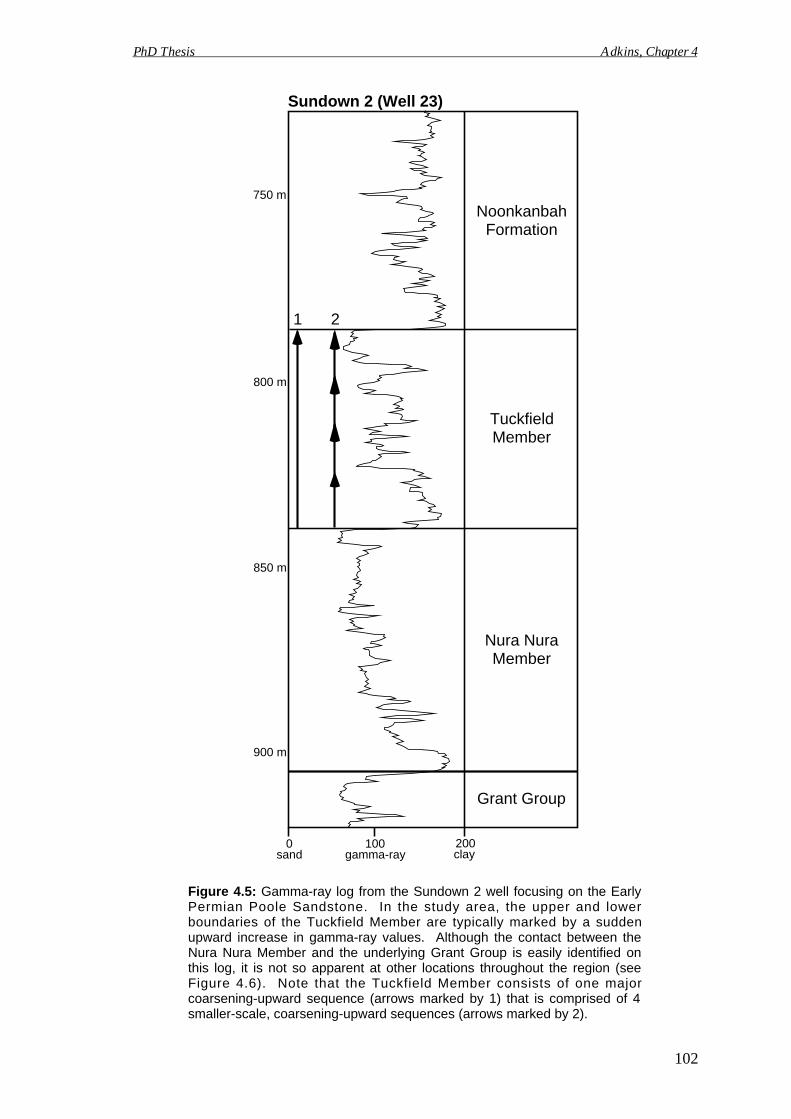
100gamma-ray
0sand
200clay
NoonkanbahFormation
TuckfieldMember
Nura NuraMember
Grant Group
Sundown 2 (Well 23)
1 2
750 m
800 m
850 m
900 m
PhD Thesis Adkins, Chapter 4
Figure 4.5: Gamma-ray log from the Sundown 2 well focusing on the EarlyPermian Poole Sandstone. In the study area, the upper and lowerboundaries of the Tuckfield Member are typically marked by a suddenupward increase in gamma-ray values. Although the contact between theNura Nura Member and the underlying Grant Group is easily identified onthis log, it is not so apparent at other locations throughout the region (seeFigure 4.6). Note that the Tuckfield Member consists of one majorcoarsening-upward sequence (arrows marked by 1) that is comprised of 4smaller-scale, coarsening-upward sequences (arrows marked by 2).
102

100gamma-ray
0 200sand clay
May River 1 Terrace 1 W. Philydrum 1 Crimson Lake 1M N
Grant Range
Lennard ShelfFitzroy Trough
100 km
124º
00'
18º00'
123º
00'
17º00'
M
NY
X
(b)
(a)
Noo
nkan
bah
Nur
a N
ura
Gra
nt
850 m
800 m
750 m
700 m
700 m
650 m
600 m
550 m800 m
850 m
900 m
950 m
500 m
550 m
600 m
?
?
?
34 km 49 km 13 km
100gamma-ray
0 200sand clay
100gamma-ray
0 200sand clay
100gamma-ray
0 200sand clay
450 m
Tuc
kfie
ld
PhD Thesis Adkins, Chapter 4
Figure 4.6: Cross-section M-N (a), labeledon map (b). This section trends oblique tothe paleo-coastline. Note that the 4 internalcoa rsen ing -upward sequences tha tcomprise the Tuckfield Member thickentowards the basin. See Figure 4.8 for cross-section X-Y.
103
Gro
upM
embe
rF
orm
atio
nM
embe
r
PhD Thesis Adkins, Chapter 4
104
(mud and shale) with minor amounts of coarser-grained sand and silt (Crowe and
Towner, 1981). These muddy deposits result in a typically high-value gamma-ray log
that is punctuated by thin, laterally discontinuous sandstone stringers that emit low
gamma-ray readings (Figures 4.5 and 4.6).
Moving deeper into the stratigraphic section, the boundary between the
Noonkanbah Formation and the Tuckfield Member is typically marked by a drastic
downward decrease in average gamma-ray values (Figures 4.5 and 4.6). This sudden
decrease marks the transition from the bottom of the muddy Noonkanbah Formation to
the top of the coarser-grained Tuckfield Member. In the study area, the Tuckfield
Member generally consists of one major coarsening-upward sequence that
systematically ranges in thickness from 39 to 68 m (Table 4.1 and Figure 4.7). As
Figure 4.7 illustrates, the Tuckfield Member gradually thickens toward the basin in a
wedge that trends roughly parallel to the trough’s northern paleo-coastline
(northwest/southeast). Within the major coarsening-upward cycle, 4 internal
coarsening-upward cycles of relatively equal thickness can also be identified (Figures
4.5 and 4.6). These internal coarsening-upward cycles thicken basinward (Figure 4.6).
Parallel to the paleo-coastline, these internal coarsening-upward cycles maintain a
relatively constant thickness and can be traced along strike for more than 200 km
(Figure 4.8).
The contact between the Tuckfield Member and the underlying Nura Nura
Member is also typically marked by a drastic downward decrease in average gamma-ray
values (Figures 4.5, 4.6, and 4.8). This gamma-ray decrease indicates a sudden
coarsening of grainsize from the base of the Tuckfield Member to the top of the Nura
Nura Member. Similar to the Tuckfield deposits, the Nura Nura deposits display a
coarsening-upward trend at some locations (e.g. Terrace 1 and Crimson Lake 1 in
Figure 4.6). Unlike the Tuckfield deposits, this coarsening-upward trend is not laterally
continuous throughout the study area (e.g. West Philydrum 1 in Figure 4.6). The lateral
variability of this unit, combined with the unconformable relationship between the Nura
Nura Member and the underlying heterogeneous Grant Group, makes it difficult to
identify the lower bounding surface of the Poole Sandstone with absolute certainty.
CYCLICITY AND SPECTRAL ANALYSES
To gain a better understanding of cyclicity recorded within the Poole Sandstone,
spectral analyses were performed on gamma-ray data from the Terrace 1 well (Table 1;
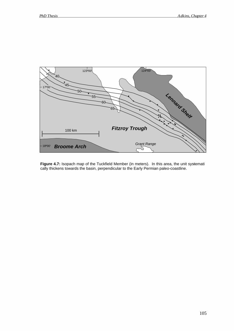
Grant Range
Lennard Shelf
Fitzroy Trough
Broome Arch
100 km
124º00'
18º00'
65
60
55
50
45
40
123º00'
17º00'
PhD Thesis Adkins, Chapter 4
Figure 4.7: Isopach map of the Tuckfield Member (in meters). In this area, the unit systemati-cally thickens towards the basin, perpendicular to the Early Permian paleo-coastline.
105
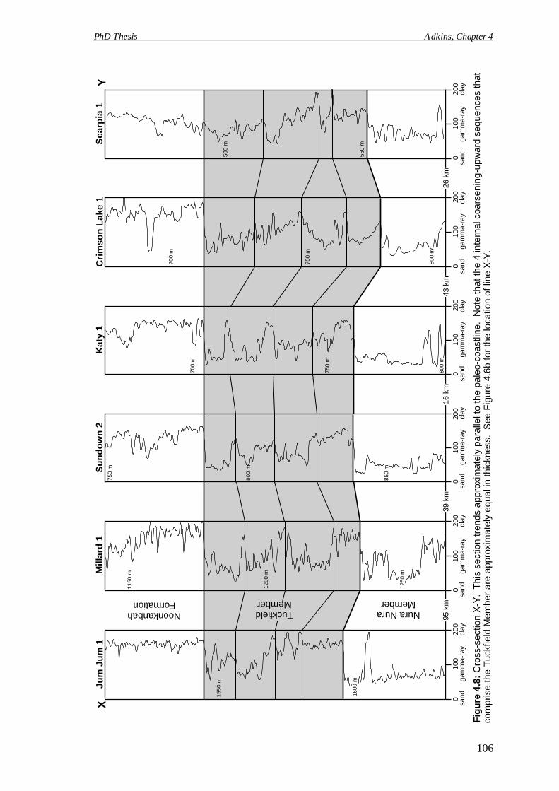
Jum
Ju
m 1
Mill
ard
1S
un
do
wn
2K
aty
1C
rim
son
Lak
e 1
Sca
rpia
1
Noonkanbah Nura Nura
95 k
m39
km
16 k
m43
km
26 k
m
1550
m
1600
m
1250
m
1200
m
1150
m
750
m
800
m
850
m
800
m
750
m
700
m
700
m
750
m
800
m
550
m
500
m
100
gam
ma-
ray
020
0sa
ndcl
ay10
0ga
mm
a-ra
y0
200
sand
clay
100
gam
ma-
ray
020
0sa
ndcl
ay10
0ga
mm
a-ra
y0
200
sand
clay
100
gam
ma-
ray
020
0sa
ndcl
ay10
0ga
mm
a-ra
y0
200
sand
clay
Tuckfield
XY
PhD Thesis Adkins, Chapter 4
Fig
ure
4.8
: C
ross
-sec
tion
X-Y
. T
his
sect
ion
tren
ds a
ppro
xim
atel
y pa
ralle
l to
the
pale
o-co
astli
ne.
Not
e th
at th
e 4
inte
rnal
coa
rsen
ing-
upw
ard
sequ
ence
s th
at
106
Formation MemberMember
com
pris
e th
e T
uckf
ield
Mem
ber
are
appr
oxim
atel
y eq
ual i
n th
ickn
ess.
See
Fig
ure
4.6b
for
the
loca
tion
of li
ne X
-Y.
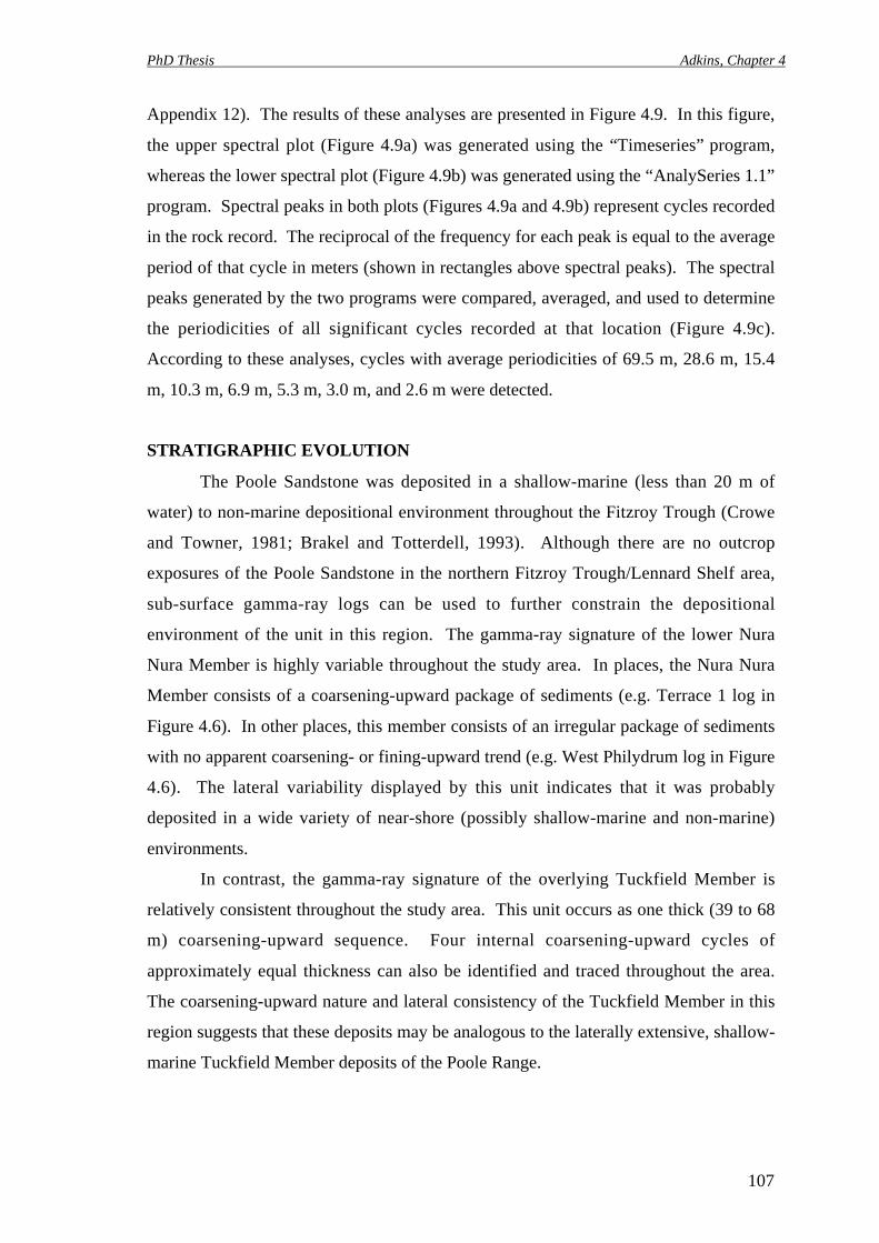
PhD Thesis Adkins, Chapter 4
107
Appendix 12). The results of these analyses are presented in Figure 4.9. In this figure,
the upper spectral plot (Figure 4.9a) was generated using the “Timeseries” program,
whereas the lower spectral plot (Figure 4.9b) was generated using the “AnalySeries 1.1”
program. Spectral peaks in both plots (Figures 4.9a and 4.9b) represent cycles recorded
in the rock record. The reciprocal of the frequency for each peak is equal to the average
period of that cycle in meters (shown in rectangles above spectral peaks). The spectral
peaks generated by the two programs were compared, averaged, and used to determine
the periodicities of all significant cycles recorded at that location (Figure 4.9c).
According to these analyses, cycles with average periodicities of 69.5 m, 28.6 m, 15.4
m, 10.3 m, 6.9 m, 5.3 m, 3.0 m, and 2.6 m were detected.
STRATIGRAPHIC EVOLUTIONThe Poole Sandstone was deposited in a shallow-marine (less than 20 m of
water) to non-marine depositional environment throughout the Fitzroy Trough (Crowe
and Towner, 1981; Brakel and Totterdell, 1993). Although there are no outcrop
exposures of the Poole Sandstone in the northern Fitzroy Trough/Lennard Shelf area,
sub-surface gamma-ray logs can be used to further constrain the depositional
environment of the unit in this region. The gamma-ray signature of the lower Nura
Nura Member is highly variable throughout the study area. In places, the Nura Nura
Member consists of a coarsening-upward package of sediments (e.g. Terrace 1 log in
Figure 4.6). In other places, this member consists of an irregular package of sediments
with no apparent coarsening- or fining-upward trend (e.g. West Philydrum log in Figure
4.6). The lateral variability displayed by this unit indicates that it was probably
deposited in a wide variety of near-shore (possibly shallow-marine and non-marine)
environments.
In contrast, the gamma-ray signature of the overlying Tuckfield Member is
relatively consistent throughout the study area. This unit occurs as one thick (39 to 68
m) coarsening-upward sequence. Four internal coarsening-upward cycles of
approximately equal thickness can also be identified and traced throughout the area.
The coarsening-upward nature and lateral consistency of the Tuckfield Member in this
region suggests that these deposits may be analogous to the laterally extensive, shallow-
marine Tuckfield Member deposits of the Poole Range.
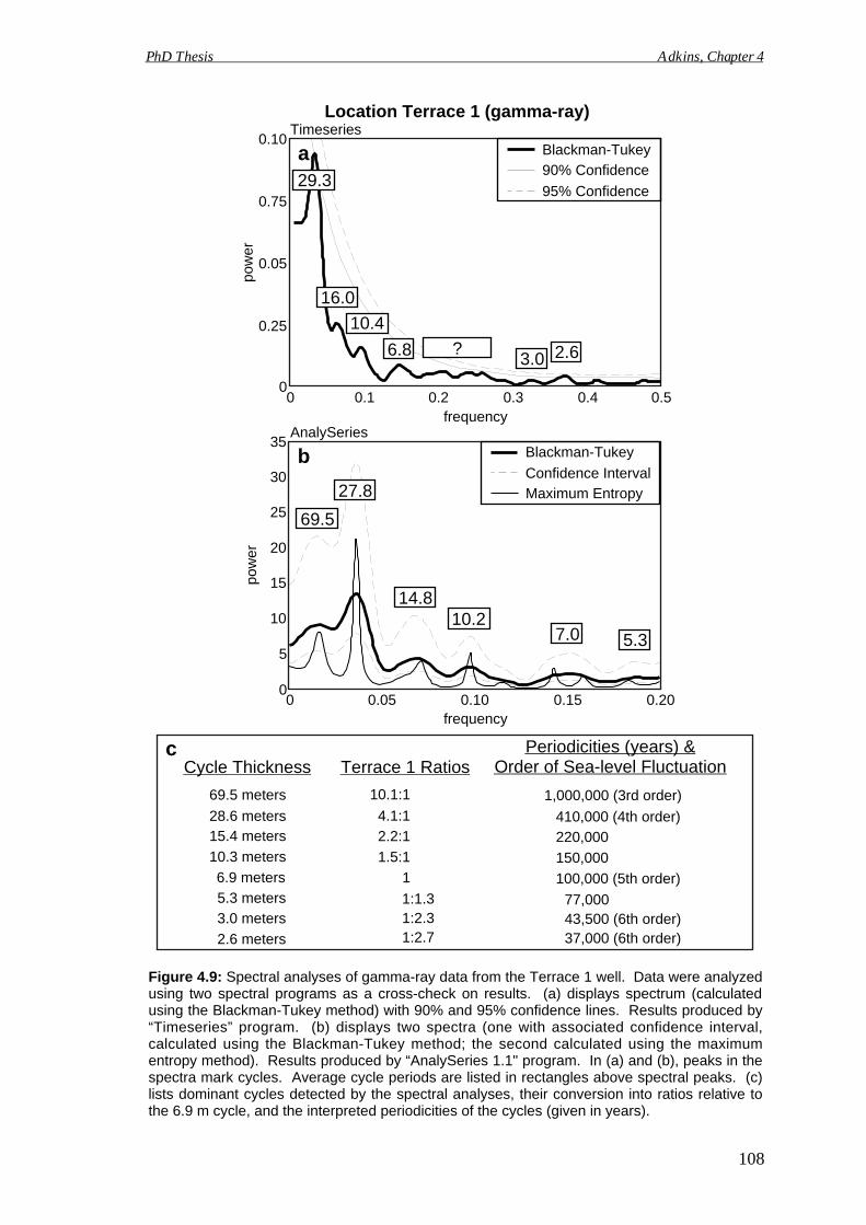
Figure 4.9: Spectral analyses of gamma-ray data from the Terrace 1 well. Data were analyzedusing two spectral programs as a cross-check on results. (a) displays spectrum (calculatedusing the Blackman-Tukey method) with 90% and 95% confidence lines. Results produced by“Timeseries” program. (b) displays two spectra (one with associated confidence interval,calculated using the Blackman-Tukey method; the second calculated using the maximumentropy method). Results produced by “AnalySeries 1.1" program. In (a) and (b), peaks in thespectra mark cycles. Average cycle periods are listed in rectangles above spectral peaks. (c)lists dominant cycles detected by the spectral analyses, their conversion into ratios relative tothe 6.9 m cycle, and the interpreted periodicities of the cycles (given in years).
0.200.150.100.0500
35Blackman-Tukey
Confidence Interval
frequency
pow
er
AnalySeries
30
20
15
10
5
Maximum Entropy
7.0 5.3
b
0 0.1 0.2 0.3 0.4 0.50
0.05
0.10Blackman-Tukey90% Confidence
95% Confidence
frequency
pow
er
Timeseries
0.75
0.25
2.6
a
cCycle Thickness
69.5 meters
28.6 meters
6.9 meters
5.3 meters
10.3 meters
15.4 meters
2.6 meters
3.0 meters
1.5:1
1
1:1.3
10.1:1
4.1:12.2:1
1:2.31:2.7
Terrace 1 Ratios
150,000
100,000 (5th order)
77,000
1,000,000 (3rd order)
410,000 (4th order)220,000
43,500 (6th order)37,000 (6th order)
Periodicities (years) &Order of Sea-level Fluctuation
Location Terrace 1 (gamma-ray)
PhD Thesis Adkins, Chapter 4
29.3
10.4
16.0
6.8
69.52527.8
14.810.2
3.0?
108
PhD Thesis Adkins, Chapter 4
To verify that the Tuckfield Member sediments in the Poole Range are indeed
analogous to the Tuckfield Member sediments in this study, gamma-ray logs from the
two areas were compared. In Figure 4.3, a lithology log with associated gamma-ray
data from the Poole Range (Location P-1, see Figure 4.1) and a gamma-ray log (Terrace
1) from the Lennard Shelf are juxtaposed. The Terrace 1 log was initially chosen
because it displays well-developed cyclicity, and more importantly, the Tuckfield
Member at this location is of a similar thickness to the Tuckfield Member in the Poole
Range. When the gamma-ray logs from the two distant areas (more than 200 km apart)
are placed side by side, it becomes apparent that there is a cycle for cycle positive
correlation between the two datasets. Therefore, it can be assumed that the Tuckfield
Member in the northern Fitzroy Trough/Lennard Shelf area consists of shallow-marine
clastic sediments that are similar in nature to those observed in the Poole Range.
Although the tectonic versus eustatic origin of cycle development remains
controversial (Miall, 1997), identified Tuckfield Member cycles from the Poole Range
have been attributed to orbitally controlled fluctuations in sea-level (Chapter 2, this
volume). This suggests that the genetically similar deposits located in the northern
Fitzroy Trough/Lennard Shelf region may record the same astronomical cycles. During
the mid-Permian, these astronomical perturbations are retrodicted to have had
periodicities of 17,600 and 21,000 years (precession); 44,000 and 35,000 years
(obliquity), 100,000 years (eccentricity), and 410,000 years (elongated eccentricity)
(Berger and Loutre, 1994). These parameters were converted into ratios by setting the
100,000 year cycle equal to one. For example, the number of 44,000 year cycles in
each 100,000 year cycle is equal to 2.3 (100,000 ÷ 44,000 = 2.3). So, the ratio used for
the 44,000 year cycle is 1:2.3. Therefore, expected Milankovitch ratios relative to the
100,000 year eccentricity cycle are: 4.1:1 (elongated eccentricity: 410,000 years); 1:2.3
(obliquity: 44,000 years); 1:2.9 (obliquity: 35,000 years); 1:4.8 (precession: 21,000
years); and 1:5.7 (precession: 17,800 years).
Spectral analyses of the Terrace 1 gamma-ray log identified several orders of
cyclicity with average periodicities of 69.5 m, 28.6 m, 15.4, m, 10.3 m, 6.9 m, 5.3 m,
3.0 m, and 2.6 m. At Location P-1 in the Poole Range, cycles averaging 6.2 m thick
were attributed to 100,000 year changes in Earth’s eccentric orbit (Chapter 2, this
volume). By assuming that the 6.9 m cycle identified on the Terrace 1 log is equivalent
to the 100,000 year eccentricity cycle from the Poole Range, average periodicities can
be calculated (in years) for all identified Terrace 1 cycles. Figure 4.9c summarizes this
109
PhD Thesis Adkins, Chapter 4
conversion (periodicities in meters to periodicities in years). Based upon these
analyses, several orders of Milankovitch-band cycles are recorded on the Terrace 1 log.
In addition to the eccentricity cycle (100,000 year/6.9 m), this log records an elongated
eccentricity cycle (410,000 year/28.6 m) and both components of mid-Permian
obliquity (43,500 year/3.0 m and 37,000 year/2.6 m).
In addition to Milankovitch-band cyclicity, other cycles were also identified on
the Terrace 1 log. Although the 10.3 m (150,000 year) cycle and the 5.3 m (77,000
year) cycle do not correspond to known astronomical periodicities, they do roughly
correspond to “extra” non-Milankovitch-band cycles that were recorded within the
Poole Range deposits (Chapter 2, this volume). These “extra” cycles have been
attributed to tectonism and/or short- to long-term changes in sediment supply (Chapter
2, this volume). The 15.4 m cycle identified on the Terrace 1 log may represent the
apparent 200,000 year cycle that was described by Hinnov (2000). And finally, the 69.5
m (1,000,000 year) cycle identified on the Terrace 1 log may record the global 3rd order
type of cyclicity that was initially described by Vail et al. (1977) and later modified by
Haq et al. (1987).
Although the identified cycles do not correspond exactly to the observed
Tuckfield Member cycles on the Terrace 1 log, it is important to remember that the data
analyzed were drawn from the upper Grant Group to the lower Noonkanbah Formation,
not just the Tuckfield Member. Therefore, cycle values reported in Figure 4.9 are
averages from the entire sequence, and do not provide specific information concerning
the Tuckfield Member. Nonetheless, they can be used as a general guideline.
In summary, the Tuckfield Member and possibly the Nura Nura Member of the
Poole Sandstone record a 3rd order global sea-level cycle. This cyclicity may be
attributed to large-scale tectonic events and/or global sea-level fluctuation associated
with the break-up of Gondwanan ice-sheets. Superimposed upon the 3rd order cyclicity
(in the Tuckfield Member and perhaps in the Nura Nura Member) are higher-frequency
Milankovitch-band cycles that record glacio-eustatic sea-level fluctuation related to the
waxing and waning of Gondwanan ice-sheets. Since much of the Fitzroy Trough was
covered by a shallow-sea during the Early Permian, cyclicity related to sea-level
fluctuation is laterally extensive throughout the basin.
110
PhD Thesis Adkins, Chapter 4
PETROLEUM POTENTIAL
Although to date the unit remains non-productive, the Early Permian Poole
Sandstone has long been identified as a potential petroleum reservoir (e.g. Jackson et
al., 1994; Apak and Carlsen, 1996). In the northern Fitzroy Trough/Lennard Shelf
region, the Poole Sandstone (particularly the Tuckfield Member) consists of a series of
laterally extensive, coarsening-upward sequences of near-shore, shallow-marine clastic
sediments. Although the reported porosity and permeability values for this unit are
limited, the data that does exist is extremely favorable. Porosities up to 42% (Havord et
al., 1997; Adkins, 2003; Chapter 1, this volume) and permeability values of up to 1700
md (Havord et al., 1997) have been reported for the Poole Sandstone. Residual oil and
fluorescence in wells located on the lower Lennard Shelf (e.g. Terrace 1) indicate that
hydrocarbons have previously passed through this unit (Havord et al., 1997).
Unfortunately, most of the wells that have been drilled in the Lennard Shelf area are
concentrated around the Beagle Bay and Pinnacle Fault Systems, suggesting that
hydrocarbon exploration has historically focused on potential structural traps.
However, offsets associated with the faults are greatest at depth and at a minimum
higher in the section (where the Poole Sandstone is located). Therefore, if
hydrocarbons do remain in the Poole Sandstone, they are probably located higher on the
Lennard Shelf, in an up-dip location. Hence, exploration of the Poole Sandstone should
focus on exploiting up-dip stratigraphic traps instead of structural traps around the
Beagle Bay and Pinnacle Fault Systems.
CONCLUSIONS
This study is the first detailed investigation into the sub-surface stratigraphic
evolution of the Early Permian Poole Sandstone. In the northern Fitzroy
Trough/Lennard Shelf region, the Poole Sandstone consists of two distinct depositional
units: the lower Nura Nura Member and the upper Tuckfield Member. In the study
area, the Tuckfield Member and possibly the Nura Nura Member consist of a 3rd order
package of predominantly shallow-marine clastic sediments. Internal cyclicity has been
noted on gamma-ray logs and identified by spectral analyses. These internal cycles are
laterally extensive and have been attributed to Milankovitch-band glacio-eustatic sea-
level fluctuations.
111
PhD Thesis Adkins, Chapter 5
Chapter 5
Shallow-marine sedimentary rhythms from the southernSydney Basin, New South Wales, Australia: a mid-
Permian record of glacio-eustacy

PhD Thesis Adkins, Chapter 5
113
ACKNOWLEDGMENT
Chapter 5 resulted from a joint project with Helen Lever. Helen assisted with the
collection of data, preliminary interpretations, and editing of the manuscript. Other than
Helen's valuable editorial comments, all text and figures presented in this chapter are
my work.
PhD Thesis Adkins, Chapter 5
114
ABSTRACT
Glacially influenced marine sediments of the Permian Pebbley Beach Formation
(Shoalhaven Group) are exposed along the coast of the southern Sydney Basin, New
South Wales, Australia. These sediments outcrop as a repetitive series of coarsening-
upward cycles that record deposition in an inner shelf to shoreface environment. At the
outcrop scale, a typical Pebbley Beach cycle consists of a 5 to 10 m thick vertical
succession of mudstone, interbedded mudstone and siltstone, and sandstone.
Superimposed upon the deposition of the repetitive, coarsening-upward cycles is the
occurrence of lonestones and diamictites, probably dropped from passing icebergs.
Although depositional cyclicity has been previously recognized in the
Shoalhaven Group, the mechanism of formation for the cycles remains poorly
understood. In this study, gamma-ray measurements were collected from outcrop
exposures of the Pebbley Beach Formation. Spectral analyses were performed on the
gamma-ray data to better define cyclicity. Results of the spectral analyses indicate that
the Pebbley Beach deposits record several orders of meter- to decameter-scale cycles.
These cycles correlate strongly with the known mid-Permian orbital periodicities of
eccentricity, obliquity, and precession. This positive correlation indicates that
Milankovitch-forcing and glacio-eustacy played a significant role in the formation of
the Pebbley Beach cycles. The recognition of Milankovitch-band cyclicity within the
Pebbley Beach Formation provides evidence that Permo-Carboniferous glaciation
extended into at least the Ufimian stage of the Late Permian.
Key Words: glacio-eustacy, late Paleozoic glaciation, Milankovitch cyclicity, Pebbley
Beach Formation, Permian, Shoalhaven Group, Sydney Basin
INTRODUCTION
Earth's climate during the latter part of the Permian (post-Sakmarian) has long
been the subject of much scientific speculation and debate. During the 1960's and
1970's, Crowell and Frakes investigated the late Paleozoic climate and paleogeography
of Gondwana (e.g. Frakes, 1969; Crowell, 1975). Based upon the occurrence of direct
glacial deposits and the recognition of worldwide glacio-eustatic cyclothems, Crowell
(1978) concluded that Permo-Carboniferous glaciation began during the Visean (Early
Carboniferous) and ended during the Kazanian (Late Permian).
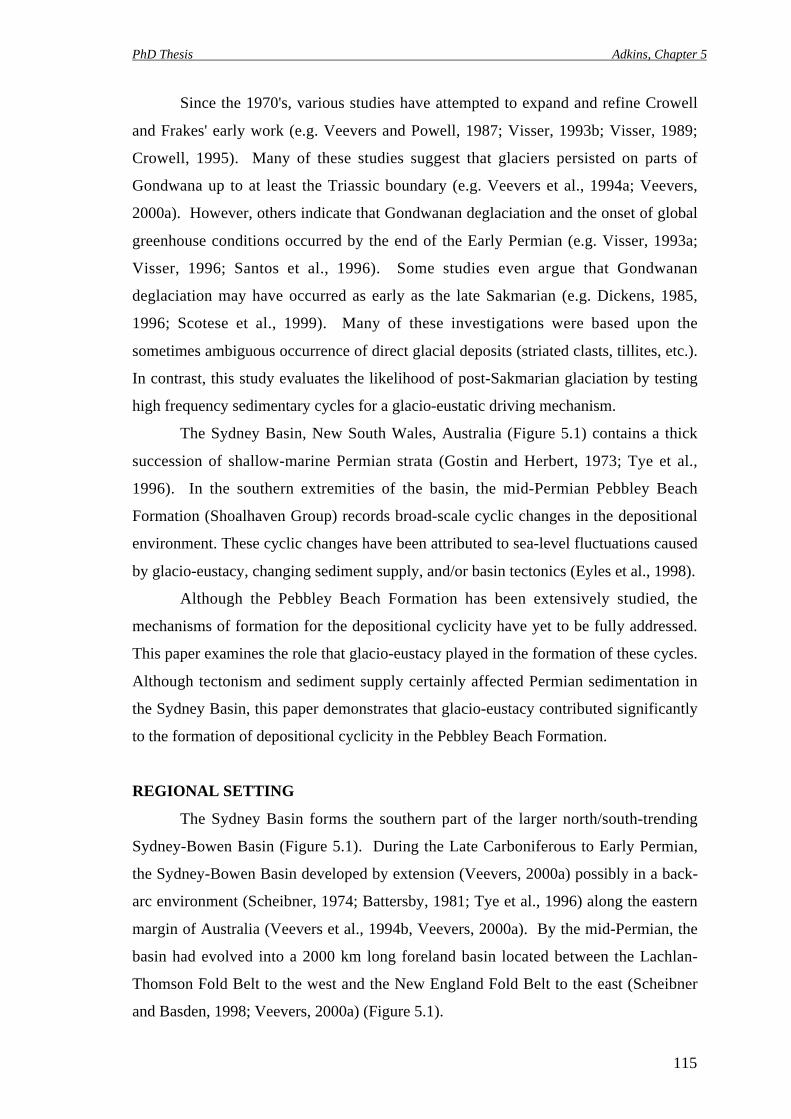
PhD Thesis Adkins, Chapter 5
115
Since the 1970's, various studies have attempted to expand and refine Crowell
and Frakes' early work (e.g. Veevers and Powell, 1987; Visser, 1993b; Visser, 1989;
Crowell, 1995). Many of these studies suggest that glaciers persisted on parts of
Gondwana up to at least the Triassic boundary (e.g. Veevers et al., 1994a; Veevers,
2000a). However, others indicate that Gondwanan deglaciation and the onset of global
greenhouse conditions occurred by the end of the Early Permian (e.g. Visser, 1993a;
Visser, 1996; Santos et al., 1996). Some studies even argue that Gondwanan
deglaciation may have occurred as early as the late Sakmarian (e.g. Dickens, 1985,
1996; Scotese et al., 1999). Many of these investigations were based upon the
sometimes ambiguous occurrence of direct glacial deposits (striated clasts, tillites, etc.).
In contrast, this study evaluates the likelihood of post-Sakmarian glaciation by testing
high frequency sedimentary cycles for a glacio-eustatic driving mechanism.
The Sydney Basin, New South Wales, Australia (Figure 5.1) contains a thick
succession of shallow-marine Permian strata (Gostin and Herbert, 1973; Tye et al.,
1996). In the southern extremities of the basin, the mid-Permian Pebbley Beach
Formation (Shoalhaven Group) records broad-scale cyclic changes in the depositional
environment. These cyclic changes have been attributed to sea-level fluctuations caused
by glacio-eustacy, changing sediment supply, and/or basin tectonics (Eyles et al., 1998).
Although the Pebbley Beach Formation has been extensively studied, the
mechanisms of formation for the depositional cyclicity have yet to be fully addressed.
This paper examines the role that glacio-eustacy played in the formation of these cycles.
Although tectonism and sediment supply certainly affected Permian sedimentation in
the Sydney Basin, this paper demonstrates that glacio-eustacy contributed significantly
to the formation of depositional cyclicity in the Pebbley Beach Formation.
REGIONAL SETTING
The Sydney Basin forms the southern part of the larger north/south-trending
Sydney-Bowen Basin (Figure 5.1). During the Late Carboniferous to Early Permian,
the Sydney-Bowen Basin developed by extension (Veevers, 2000a) possibly in a back-
arc environment (Scheibner, 1974; Battersby, 1981; Tye et al., 1996) along the eastern
margin of Australia (Veevers et al., 1994b, Veevers, 2000a). By the mid-Permian, the
basin had evolved into a 2000 km long foreland basin located between the Lachlan-
Thomson Fold Belt to the west and the New England Fold Belt to the east (Scheibner
and Basden, 1998; Veevers, 2000a) (Figure 5.1).
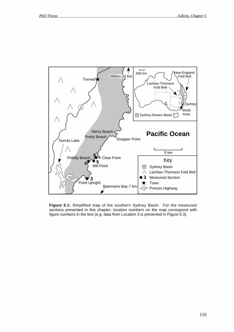
1
Termeil
Pacific OceanMerry BeachPretty Beach
Snapper Point
Clear Point
Mill Point
Point Upright
Pebbly Beach
Durras Lake
3
4 5
6
Sydney Basin
Measured Section3Lachlan-Thomson Fold Belt
Princes Highway1
Town
Key
5 km
Batemans Bay-7 km
Sydney-Bowen Basin
500 km
Sydney
Study
New England
Lachlan-Thomson
Milton-20 km
Figure 5.1: Simplified map of the southern Sydney Basin. For the measuredsections presented in this chapter, location numbers on the map correspond withfigure numbers in the text (e.g. data from Location 3 is presented in Figure 5.3).
PhD Thesis Adkins, Chapter 5
116
Fold Belt
Fold Belt
Area
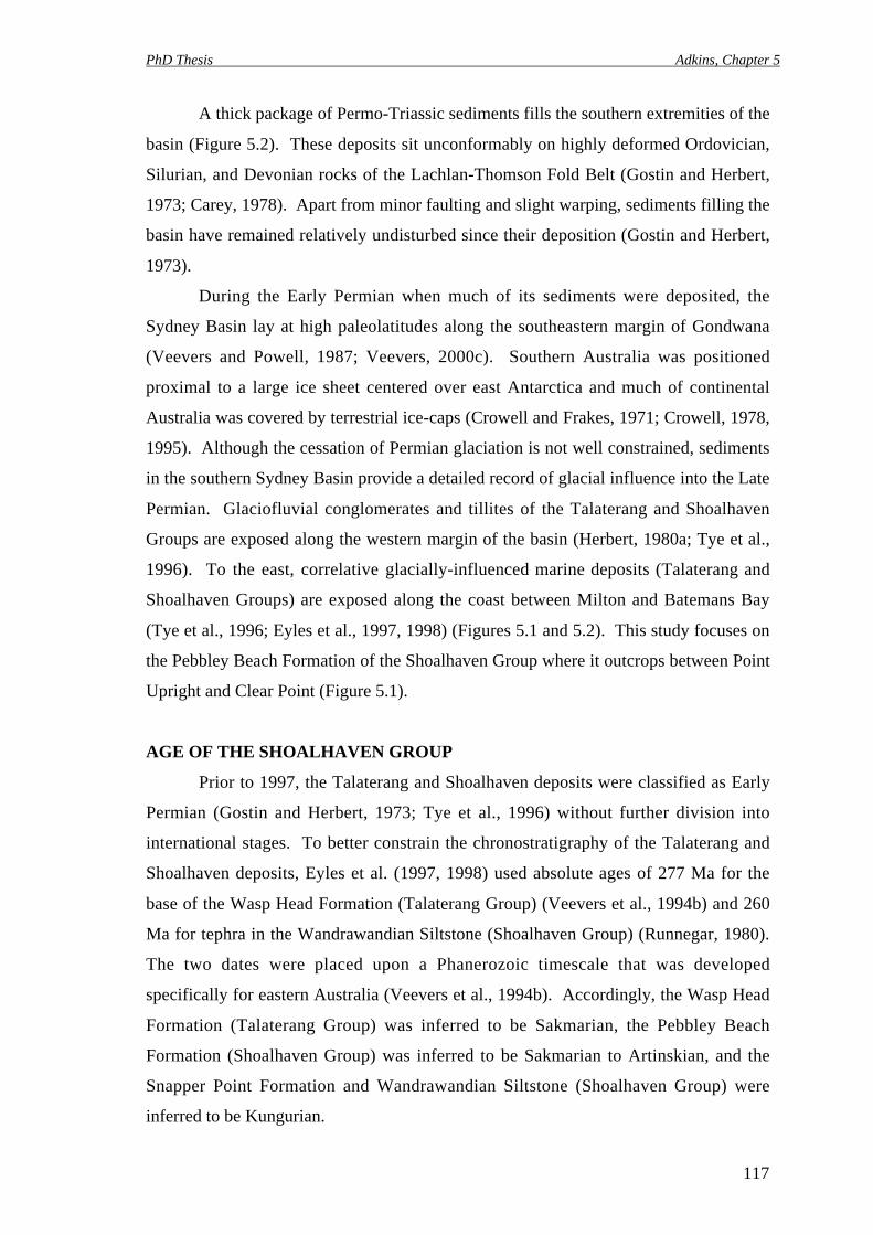
PhD Thesis Adkins, Chapter 5
117
A thick package of Permo-Triassic sediments fills the southern extremities of the
basin (Figure 5.2). These deposits sit unconformably on highly deformed Ordovician,
Silurian, and Devonian rocks of the Lachlan-Thomson Fold Belt (Gostin and Herbert,
1973; Carey, 1978). Apart from minor faulting and slight warping, sediments filling the
basin have remained relatively undisturbed since their deposition (Gostin and Herbert,
1973).
During the Early Permian when much of its sediments were deposited, the
Sydney Basin lay at high paleolatitudes along the southeastern margin of Gondwana
(Veevers and Powell, 1987; Veevers, 2000c). Southern Australia was positioned
proximal to a large ice sheet centered over east Antarctica and much of continental
Australia was covered by terrestrial ice-caps (Crowell and Frakes, 1971; Crowell, 1978,
1995). Although the cessation of Permian glaciation is not well constrained, sediments
in the southern Sydney Basin provide a detailed record of glacial influence into the Late
Permian. Glaciofluvial conglomerates and tillites of the Talaterang and Shoalhaven
Groups are exposed along the western margin of the basin (Herbert, 1980a; Tye et al.,
1996). To the east, correlative glacially-influenced marine deposits (Talaterang and
Shoalhaven Groups) are exposed along the coast between Milton and Batemans Bay
(Tye et al., 1996; Eyles et al., 1997, 1998) (Figures 5.1 and 5.2). This study focuses on
the Pebbley Beach Formation of the Shoalhaven Group where it outcrops between Point
Upright and Clear Point (Figure 5.1).
AGE OF THE SHOALHAVEN GROUP
Prior to 1997, the Talaterang and Shoalhaven deposits were classified as Early
Permian (Gostin and Herbert, 1973; Tye et al., 1996) without further division into
international stages. To better constrain the chronostratigraphy of the Talaterang and
Shoalhaven deposits, Eyles et al. (1997, 1998) used absolute ages of 277 Ma for the
base of the Wasp Head Formation (Talaterang Group) (Veevers et al., 1994b) and 260
Ma for tephra in the Wandrawandian Siltstone (Shoalhaven Group) (Runnegar, 1980).
The two dates were placed upon a Phanerozoic timescale that was developed
specifically for eastern Australia (Veevers et al., 1994b). Accordingly, the Wasp Head
Formation (Talaterang Group) was inferred to be Sakmarian, the Pebbley Beach
Formation (Shoalhaven Group) was inferred to be Sakmarian to Artinskian, and the
Snapper Point Formation and Wandrawandian Siltstone (Shoalhaven Group) were
inferred to be Kungurian.
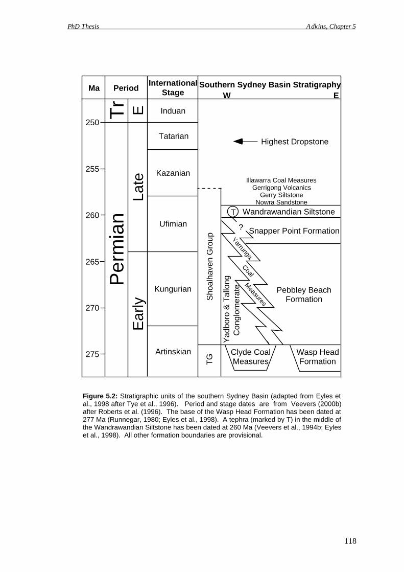
Figure 5.2: Stratigraphic units of the southern Sydney Basin (adapted from Eyles etal., 1998 after Tye et al., 1996). Period and stage dates are from Veevers (2000b)after Roberts et al. (1996). The base of the Wasp Head Formation has been dated at277 Ma (Runnegar, 1980; Eyles et al., 1998). A tephra (marked by T) in the middle ofthe Wandrawandian Siltstone has been dated at 260 Ma (Veevers et al., 1994b; Eyleset al., 1998). All other formation boundaries are provisional.
Artinskian
Kungurian
Ufimian
Per
mia
n Wandrawandian SiltstoneT
Pebbley Beach
Snapper Point Formation
Wasp Head
TG
Sho
alha
ven
Gro
up260
265
270
275
Ma PeriodInternational Southern Sydney Basin Stratigraphy
255
250T
rE
arly
Late
E
Kazanian
TatarianHighest Dropstone
Nowra SandstoneGerry Siltstone
Gerrigong VolcanicsIllawarra Coal Measures
W E
Clyde Coal
Yad
boro
& T
allo
ng
YarrungaCoal
Measures
?
Induan
PhD Thesis Adkins, Chapter 5
118
Stage
Formation
Con
glom
erat
e
FormationMeasures
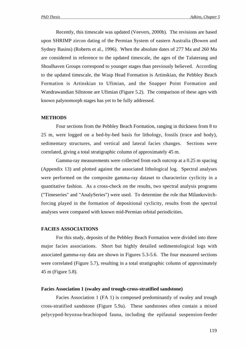
PhD Thesis Adkins, Chapter 5
119
Recently, this timescale was updated (Veevers, 2000b). The revisions are based
upon SHRIMP zircon dating of the Permian System of eastern Australia (Bowen and
Sydney Basins) (Roberts et al., 1996). When the absolute dates of 277 Ma and 260 Ma
are considered in reference to the updated timescale, the ages of the Talaterang and
Shoalhaven Groups correspond to younger stages than previously believed. According
to the updated timescale, the Wasp Head Formation is Artinskian, the Pebbley Beach
Formation is Artinskian to Ufimian, and the Snapper Point Formation and
Wandrawandian Siltstone are Ufimian (Figure 5.2). The comparison of these ages with
known palynomorph stages has yet to be fully addressed.
METHODS
Four sections from the Pebbley Beach Formation, ranging in thickness from 8 to
25 m, were logged on a bed-by-bed basis for lithology, fossils (trace and body),
sedimentary structures, and vertical and lateral facies changes. Sections were
correlated, giving a total stratigraphic column of approximately 45 m.
Gamma-ray measurements were collected from each outcrop at a 0.25 m spacing
(Appendix 13) and plotted against the associated lithological log. Spectral analyses
were performed on the composite gamma-ray dataset to characterize cyclicity in a
quantitative fashion. As a cross-check on the results, two spectral analysis programs
("Timeseries" and "AnalySeries") were used. To determine the role that Milankovitch-
forcing played in the formation of depositional cyclicity, results from the spectral
analyses were compared with known mid-Permian orbital periodicities.
FACIES ASSOCIATIONS
For this study, deposits of the Pebbley Beach Formation were divided into three
major facies associations. Short but highly detailed sedimentological logs with
associated gamma-ray data are shown in Figures 5.3-5.6. The four measured sections
were correlated (Figure 5.7), resulting in a total stratigraphic column of approximately
45 m (Figure 5.8).
Facies Association 1 (swaley and trough-cross-stratified sandstone)
Facies Association 1 (FA 1) is composed predominantly of swaley and trough
cross-stratified sandstone (Figure 5.9a). These sandstones often contain a mixed
pelycypod-bryozoa-brachiopod fauna, including the epifaunal suspension-feeder
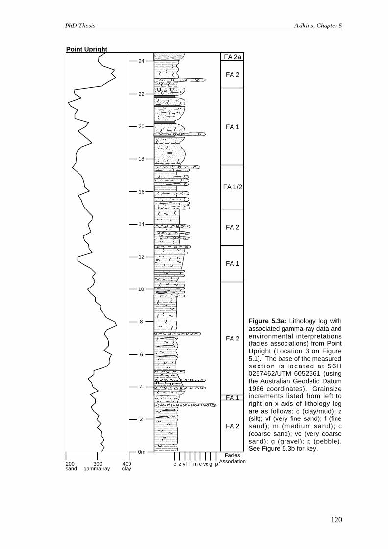
200 300 400sand claygamma-ray
0m
2
4
6
8
10
12
14
16
18
20
22
24
c z vf f m c vc g p
FaciesAssociation
FA 2a
FA 2
FA 1
FA 1/2
FA 2
FA 1
FA 2
FA 1
FA 2
Point Upright
Figure 5.3a: Lithology log withassociated gamma-ray data andenvironmental interpretations(facies associations) from PointUpright (Location 3 on Figure5.1). The base of the measureds e c t i o n i s l o c a t e d a t 5 6 H0257462/UTM 6052561 (usingthe Australian Geodetic Datum1966 coordinates). Grainsizeincrements listed from left toright on x-axis of lithology logare as follows: c (clay/mud); z(silt); vf (very fine sand); f (finesand); m (medium sand); c(coarse sand); vc (very coarsesand); g (gravel); p (pebble).See Figure 5.3b for key.
PhD Thesis Adkins, Chapter 5
120
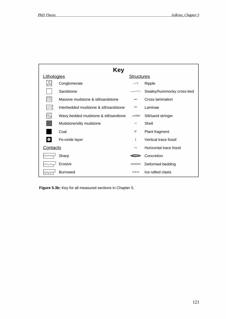
Mudstone/silty mudstone
Coal
Sandstone
Conglomerate
Massive mudstone & silt/sandstone
Fe Fe-oxide layer
Interbedded mudstone & silt/sandstone
Wavy bedded mudstone & silt/sandtone
Lithologies
Sharp
Erosive
Burrowed
Contacts
Swaley/hummocky cross-bed
Ripple
Cross lamination
Silt/sand stringer
Horizontal trace fossil
Vertical trace fossil
Shell
Laminae
Plant fragment
Deformed bedding
Ice-rafted clasts
Concretion
StructuresKey
Figure 5.3b: Key for all measured sections in Chapter 5.
PhD Thesis Adkins, Chapter 5
121
8
6
4
2
0m
200 300 400sand gamma-ray clay
c z vf f m c vc p
FaciesAssociationg
FA2
FA1
FA2
Figure 5.4: Lithology log with associated gamma-ray data andenvironmental interpretations (facies associations) from southof Pebbly Beach (Location 4 on Figure 5.1). The base of themeasured section is located at 56H 0257527/UTM 6055617(using the Australian Geodetic Datum 1966 coordinates). Keyas in Figure 5.3b.
PhD Thesis Adkins, Chapter 5
Pebbly Beach
122
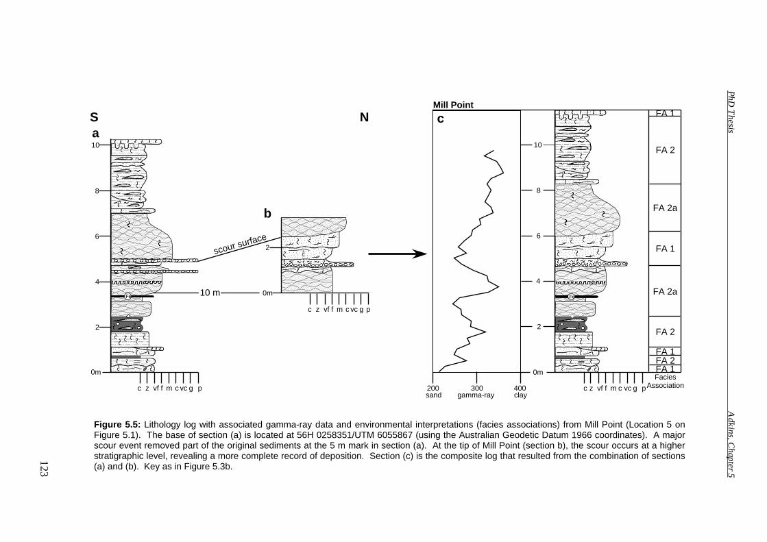
Fe
200 300 400sand gamma-ray clay
c z vf f m c vc g p
0m
2
4
6
8
10
FaciesAssociation
FA 1
FA 2
FA 2a
FA 1
FA 2a
FA 2
FA 1FA 2FA 1
c z vf f m c vc g p
0m
2
4
6
8
10
0m
2
c z vf f m c vc g p
10 m
scour surface
Fe
S Na
b
c
Figure 5.5: Lithology log with associated gamma-ray data and environmental interpretations (facies associations) from Mill Point (Location 5 onFigure 5.1). The base of section (a) is located at 56H 0258351/UTM 6055867 (using the Australian Geodetic Datum 1966 coordinates). A majorscour event removed part of the original sediments at the 5 m mark in section (a). At the tip of Mill Point (section b), the scour occurs at a higherstratigraphic level, revealing a more complete record of deposition. Section (c) is the composite log that resulted from the combination of sections(a) and (b). Key as in Figure 5.3b.
Mill Point
PhD T
hesis
Adkins, C
hapter 5
123
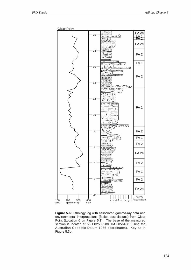
Fe
100 200 300 400sand gamma-ray clay
c z vf f m c vc g p
0m
2
4
6
8
10
12
14
16
18
20
FaciesAssociation
FA 2a
FA 2
FA 1
FA 2
FA 2a
FA 2
FA 1
FA 2
FA 1
FA 2
FA 1
FA 2
FA 2a
FA 2FA 1FA 2a
Clear Point
PhD Thesis Adkins, Chapter 5
Figure 5.6: Lithology log with associated gamma-ray data andenvironmental interpretations (facies associations) from ClearPoint (Location 6 on Figure 5.1). The base of the measuredsection is located at 56H 0258658/UTM 6056430 (using theAustralian Geodetic Datum 1966 coordinates). Key as inFigure 5.3b.
124

2.75 km
3.5 km
0.75 km
scour surface
a
*
b
c
*
0 m
4
2
dS N
Figure 5.7: Correlation ofPebbley Beach sections.(a) is from Point Upright(Figure 5.3). (b) is fromsou th o f Pebb l y Beach(Figure 5.4). (c) is from MillPoint (Figure 5.5). (d) isfrom Clear Point (Figure5.6). Sections marked by (*)are discussed in the text(under Milankovitch-bandCyclicity). Key as in Figure5.3b.
PhD Thesis Adkins, Chapter 5
125
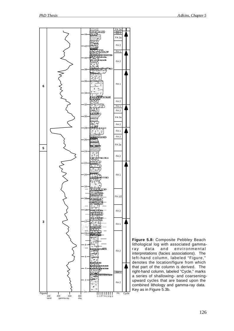
100 300200 400sand claygamma-ray
0m
2
4
6
8
10
12
14
16
18
20
22
24
c z vf f m c vcg pFA
FA 2
FA 1
FA 1/2
FA 2
FA 1
FA 2
FA 1
FA 2
FA 2a
26
28
30
32
34
36
38
40
42
44
FA 2
FA 1
FA 2
FA 2a
FA 2
FA 1
FA 2
FA 1
FA 2
FA 1
FA 2
FA 2a
FA 2FA 1FA 2a
Figure
6
5
3
Cycle
Figure 5.8: Composite Pebbley Beachlithological log with associated gamma-r a y d a t a a n d e n v i r o n m e n t a linterpretations (facies associations). Thelef t-hand column, labeled “Figure,”denotes the location/figure from whichthat part of the column is derived. Theright-hand column, labeled “Cycle,” marksa series of shallowing- and coarsening-upward cycles that are based upon thecombined lithology and gamma-ray data.Key as in Figure 5.3b.
PhD Thesis Adkins, Chapter 5
126
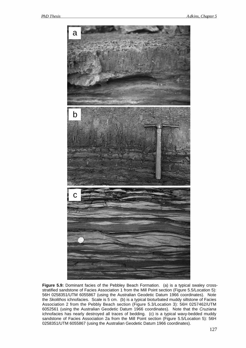
Figure 5.9: Dominant facies of the Pebbley Beach Formation. (a) is a typical swaley cross-stratified sandstone of Facies Association 1 from the Mill Point section (Figure 5.5/Location 5):56H 0258351/UTM 6055867 (using the Australian Geodetic Datum 1966 coordinates). Notethe Skolithos ichnofacies. Scale is 5 cm. (b) is a typical bioturbated muddy siltstone of FaciesAssociation 2 from the Pebbly Beach section (Figure 5.3/Location 3): 56H 0257462/UTM6052561 (using the Australian Geodetic Datum 1966 coordinates). Note that the Cruzianaichnofacies has nearly destroyed all traces of bedding. (c) is a typical wavy-bedded muddysandstone of Facies Association 2a from the Mill Point section (Figure 5.5/Location 5): 56H0258351/UTM 6055867 (using the Australian Geodetic Datum 1966 coordinates).
a
b
c
PhD Thesis Adkins, Chapter 5
127
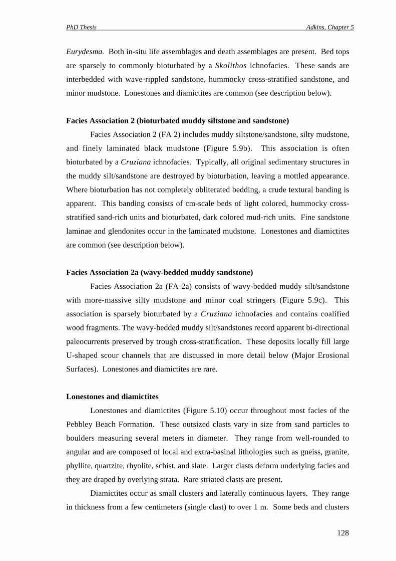
PhD Thesis Adkins, Chapter 5
128
Eurydesma. Both in-situ life assemblages and death assemblages are present. Bed tops
are sparsely to commonly bioturbated by a Skolithos ichnofacies. These sands are
interbedded with wave-rippled sandstone, hummocky cross-stratified sandstone, and
minor mudstone. Lonestones and diamictites are common (see description below).
Facies Association 2 (bioturbated muddy siltstone and sandstone)
Facies Association 2 (FA 2) includes muddy siltstone/sandstone, silty mudstone,
and finely laminated black mudstone (Figure 5.9b). This association is often
bioturbated by a Cruziana ichnofacies. Typically, all original sedimentary structures in
the muddy silt/sandstone are destroyed by bioturbation, leaving a mottled appearance.
Where bioturbation has not completely obliterated bedding, a crude textural banding is
apparent. This banding consists of cm-scale beds of light colored, hummocky cross-
stratified sand-rich units and bioturbated, dark colored mud-rich units. Fine sandstone
laminae and glendonites occur in the laminated mudstone. Lonestones and diamictites
are common (see description below).
Facies Association 2a (wavy-bedded muddy sandstone)
Facies Association 2a (FA 2a) consists of wavy-bedded muddy silt/sandstone
with more-massive silty mudstone and minor coal stringers (Figure 5.9c). This
association is sparsely bioturbated by a Cruziana ichnofacies and contains coalified
wood fragments. The wavy-bedded muddy silt/sandstones record apparent bi-directional
paleocurrents preserved by trough cross-stratification. These deposits locally fill large
U-shaped scour channels that are discussed in more detail below (Major Erosional
Surfaces). Lonestones and diamictites are rare.
Lonestones and diamictites
Lonestones and diamictites (Figure 5.10) occur throughout most facies of the
Pebbley Beach Formation. These outsized clasts vary in size from sand particles to
boulders measuring several meters in diameter. They range from well-rounded to
angular and are composed of local and extra-basinal lithologies such as gneiss, granite,
phyllite, quartzite, rhyolite, schist, and slate. Larger clasts deform underlying facies and
they are draped by overlying strata. Rare striated clasts are present.
Diamictites occur as small clusters and laterally continuous layers. They range
in thickness from a few centimeters (single clast) to over 1 m. Some beds and clusters
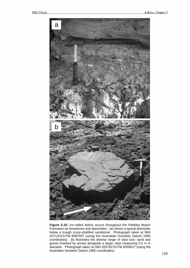
b
a
Figure 5.10: Ice-rafted debris occurs throughout the Pebbley BeachFormation as lonestones and diamictites. (a) shows a typical diamictitebelow a trough cross-stratified sandstone. Photograph taken at 56H0271321/UTM 6087697 (using the Australian Geodetic Datum 1966coordinates). (b) illustrates the diverse range of clast size: sand andgravel (marked by arrow) alongside a larger clast measuring 0.5 m indiameter. Photograph taken at 56H 0257527/UTM 6055617 (using theAustralian Geodetic Datum 1966 coordinates).
PhD Thesis Adkins, Chapter 5
129
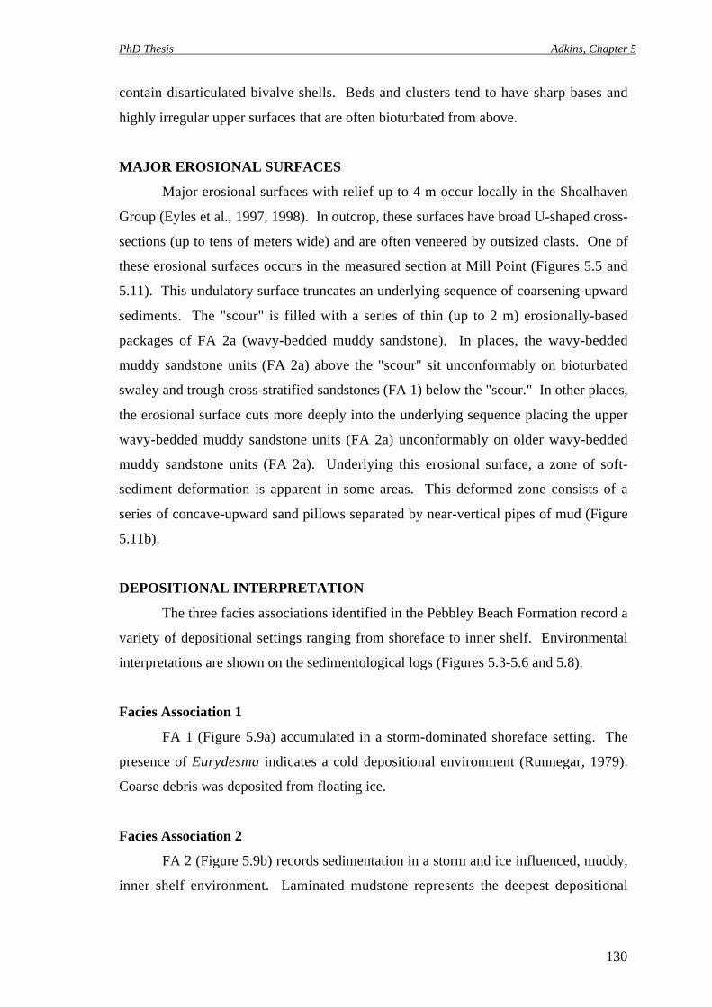
PhD Thesis Adkins, Chapter 5
130
contain disarticulated bivalve shells. Beds and clusters tend to have sharp bases and
highly irregular upper surfaces that are often bioturbated from above.
MAJOR EROSIONAL SURFACES
Major erosional surfaces with relief up to 4 m occur locally in the Shoalhaven
Group (Eyles et al., 1997, 1998). In outcrop, these surfaces have broad U-shaped cross-
sections (up to tens of meters wide) and are often veneered by outsized clasts. One of
these erosional surfaces occurs in the measured section at Mill Point (Figures 5.5 and
5.11). This undulatory surface truncates an underlying sequence of coarsening-upward
sediments. The "scour" is filled with a series of thin (up to 2 m) erosionally-based
packages of FA 2a (wavy-bedded muddy sandstone). In places, the wavy-bedded
muddy sandstone units (FA 2a) above the "scour" sit unconformably on bioturbated
swaley and trough cross-stratified sandstones (FA 1) below the "scour." In other places,
the erosional surface cuts more deeply into the underlying sequence placing the upper
wavy-bedded muddy sandstone units (FA 2a) unconformably on older wavy-bedded
muddy sandstone units (FA 2a). Underlying this erosional surface, a zone of soft-
sediment deformation is apparent in some areas. This deformed zone consists of a
series of concave-upward sand pillows separated by near-vertical pipes of mud (Figure
5.11b).
DEPOSITIONAL INTERPRETATION
The three facies associations identified in the Pebbley Beach Formation record a
variety of depositional settings ranging from shoreface to inner shelf. Environmental
interpretations are shown on the sedimentological logs (Figures 5.3-5.6 and 5.8).
Facies Association 1
FA 1 (Figure 5.9a) accumulated in a storm-dominated shoreface setting. The
presence of Eurydesma indicates a cold depositional environment (Runnegar, 1979).
Coarse debris was deposited from floating ice.
Facies Association 2
FA 2 (Figure 5.9b) records sedimentation in a storm and ice influenced, muddy,
inner shelf environment. Laminated mudstone represents the deepest depositional
scour
a
b
Figure 5.11: Major erosional surface at Mill Point (Figure 5.5/Location 5):56H 0258351/UTM 6055867 (using the Australian Geodetic Datum 1966coordinates). This scour may record an episode of iceberg grounding. (a)shows the erosional surface cutting into underlying sediments of acoarsening-upward sequence. (b) shows a zone of deformation underlyingthe scour surface. Note the concave-upward sand pillows separated by anear-vertical pipe of mud. The scale in both photographs is 1.5 m.
PhD Thesis Adkins, Chapter 5
131
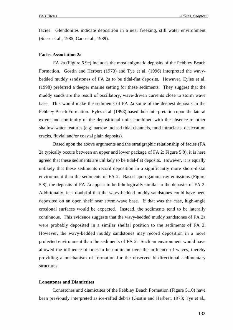
PhD Thesis Adkins, Chapter 5
132
facies. Glendonites indicate deposition in a near freezing, still water environment
(Suess et al., 1985; Carr et al., 1989).
Facies Association 2a
FA 2a (Figure 5.9c) includes the most enigmatic deposits of the Pebbley Beach
Formation. Gostin and Herbert (1973) and Tye et al. (1996) interpreted the wavy-
bedded muddy sandstones of FA 2a to be tidal-flat deposits. However, Eyles et al.
(1998) preferred a deeper marine setting for these sediments. They suggest that the
muddy sands are the result of oscillatory, wave-driven currents close to storm wave
base. This would make the sediments of FA 2a some of the deepest deposits in the
Pebbley Beach Formation. Eyles et al. (1998) based their interpretation upon the lateral
extent and continuity of the depositional units combined with the absence of other
shallow-water features (e.g. narrow incised tidal channels, mud intraclasts, desiccation
cracks, fluvial and/or coastal plain deposits).
Based upon the above arguments and the stratigraphic relationship of facies (FA
2a typically occurs between an upper and lower package of FA 2: Figure 5.8), it is here
agreed that these sediments are unlikely to be tidal-flat deposits. However, it is equally
unlikely that these sediments record deposition in a significantly more shore-distal
environment than the sediments of FA 2. Based upon gamma-ray emissions (Figure
5.8), the deposits of FA 2a appear to be lithologically similar to the deposits of FA 2.
Additionally, it is doubtful that the wavy-bedded muddy sandstones could have been
deposited on an open shelf near storm-wave base. If that was the case, high-angle
erosional surfaces would be expected. Instead, the sediments tend to be laterally
continuous. This evidence suggests that the wavy-bedded muddy sandstones of FA 2a
were probably deposited in a similar shelfal position to the sediments of FA 2.
However, the wavy-bedded muddy sandstones may record deposition in a more
protected environment than the sediments of FA 2. Such an environment would have
allowed the influence of tides to be dominant over the influence of waves, thereby
providing a mechanism of formation for the observed bi-directional sedimentary
structures.
Lonestones and Diamictites
Lonestones and diamictites of the Pebbley Beach Formation (Figure 5.10) have
been previously interpreted as ice-rafted debris (Gostin and Herbert, 1973; Tye et al.,
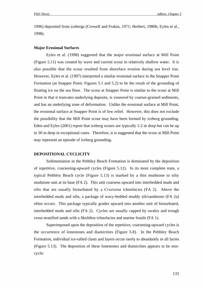
PhD Thesis Adkins, Chapter 5
133
1996) deposited from icebergs (Crowell and Frakes, 1971; Herbert, 1980b; Eyles et al.,
1998).
Major Erosional Surfaces
Eyles et al. (1998) suggested that the major erosional surface at Mill Point
(Figure 5.11) was created by wave and current scour in relatively shallow water. It is
also possible that the scour resulted from shoreface erosion during sea level rise.
However, Eyles et al. (1997) interpreted a similar erosional surface in the Snapper Point
Formation (at Snapper Point: Figures 5.1 and 5.2) to be the result of the grounding of
floating ice on the sea floor. The scour at Snapper Point is similar to the scour at Mill
Point in that it truncates underlying deposits, is veneered by coarser-grained sediments,
and has an underlying zone of deformation. Unlike the erosional surface at Mill Point,
the erosional surface at Snapper Point is of low relief. However, this does not exclude
the possibility that the Mill Point scour may have been formed by iceberg grounding.
Eden and Eyles (2001) report that iceberg scours are typically 1-2 m deep but can be up
to 30 m deep in exceptional cases. Therefore, it is suggested that the scour at Mill Point
may represent an episode of iceberg grounding.
DEPOSITIONAL CYCLICITY
Sedimentation in the Pebbley Beach Formation is dominated by the deposition
of repetitive, coarsening-upward cycles (Figure 5.12). In its most complete state, a
typical Pebbley Beach cycle (Figure 5.13) is marked by a thin mudstone to silty
mudstone unit at its base (FA 2). This unit coarsens upward into interbedded muds and
silts that are usually bioturbated by a Cruziana ichnofacies (FA 2). Above the
interbedded muds and silts, a package of wavy-bedded muddy silt/sandstone (FA 2a)
often occurs. This package typically grades upward into another unit of bioturbated,
interbedded muds and silts (FA 2). Cycles are usually capped by swaley and trough
cross-stratified sands with a Skolithos ichnofacies and marine fossils (FA 1).
Superimposed upon the deposition of the repetitive, coarsening-upward cycles is
the occurrence of lonestones and diamictites (Figure 5.8). In the Pebbley Beach
Formation, individual ice-rafted clasts and layers occur rarely to abundantly in all facies
(Figure 5.13). The deposition of these lonestones and diamictites appears to be non-
cyclic
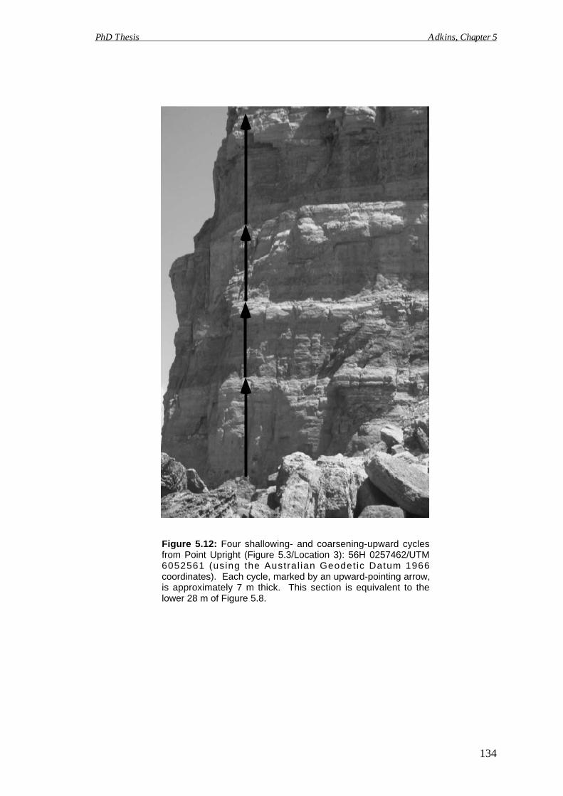
Figure 5.12: Four shallowing- and coarsening-upward cyclesfrom Point Upright (Figure 5.3/Location 3): 56H 0257462/UTM6052561 (using the Austral ian Geodet ic Datum 1966coordinates). Each cycle, marked by an upward-pointing arrow,is approximately 7 m thick. This section is equivalent to thelower 28 m of Figure 5.8.
PhD Thesis Adkins, Chapter 5
134
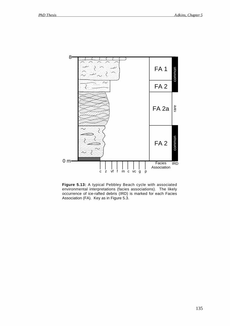
8
0 m
f vcc z m gcvf p
FA 2
FA 2a
FA 2
FA 1
FaciesAssociation
Figure 5.13: A typical Pebbley Beach cycle with associatedenvironmental interpretations (facies associations). The likelyoccurrence of ice-rafted debris (IRD) is marked for each FaciesAssociation (FA). Key as in Figure 5.3.
IRD
PhD Thesis Adkins, Chapter 5
135
com
mon
rare
com
mon
PhD Thesis Adkins, Chapter 5
136
Figure 5.8 demonstrates the repetitive nature of Pebbley Beach cycles. Inner
shelf deposits of FA 2 and 2a repeatedly shallow and coarsen upward to the shoreface
deposits of FA 1. This same trend can be seen on the composite gamma-ray log (Figure
5.8). Upward-pointing arrows in Figure 5.8 denote eight successive coarsening-upward
cycles. Complete cycles occur in the upper half of the composite section (Figure 5.8).
In the lower half, FA 2a is absent indicating that an open-shelf environment prevailed
during this time. Cycle boundaries are based upon the combined lithological and
gamma-ray data. These boundaries are often marked by an abrupt drowning event that
places muddy inner shelf deposits with higher gamma-ray values on top of sandy
shoreface deposits with lower gamma-ray values. The lower 28 m of Figure 5.8 are
approximately equivalent to the four cycles shown in Figure 5.12.
SPECTRAL ANALYSIS
Spectral analysis is an objective, statistical method for detecting cyclicity in a
dataset. It is particularly useful because it is able to differentiate regular cycles from
random events. The composite gamma-ray log from the Pebbley Beach Formation
(Figure 5.8) was analyzed for cyclicity using two spectral analysis programs (Figure
5.14). Results generated by "Timeseries" (Weedon and Read, 1995) are shown in
Figure 5.14a. Results generated by "AnalySeries 1.1" (Paillard et al., 1996), are shown
in Figure 5.14b. Peaks in the spectra (Figures 5.14a and 5.14b) represent cycles
recorded in the rock record. The reciprocal of the frequency for each peak is equal to its
average cycle period in meters. Spectral peaks generated by the two programs were
compared, averaged, and used to determine the periodicities of all significant cycles
(Figure 5.14c). For example, the 9.0 m cycle in Figure 5.14a was averaged with the 8.0
m cycle in Figure 5.14b to obtain an average cycle thickness of 8.5 m (Figure 5.14c).
According to these analyses, several orders of cyclicity with average periods of 19.7 m,
8.5 m, 4.9 m, 3.2 m, 1.8 m and 1.3 m are recorded in the Pebbley Beach deposits.
MILANKOVITCH CYCLICITY
Milankovitch cycle is a term used to describe any cycle that is caused by
changes in Earth's orbital elements. Milankovitch-scale cyclicity is often recorded in
the rock record as high-frequency sedimentary cycles (i.e. cyclothems: Abbott and
Carter, 1994). This is possible because cyclic changes in Earth's orbit cause climatic
fluctuations that affect the distribution of radiation reaching Earth's atmosphere. These
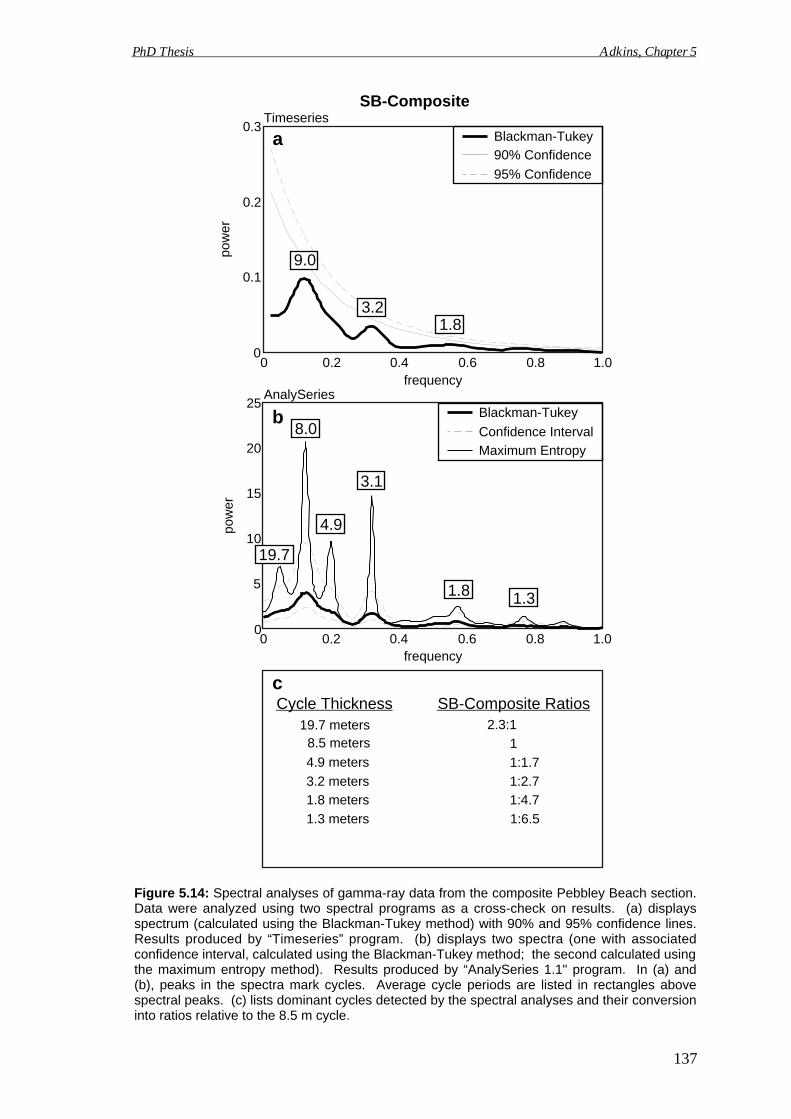
0
10
15
25Blackman-Tukey
Confidence Interval
frequency
pow
er
AnalySeries
5
20 Maximum Entropy
3.1
19.7
0 0.2 0.4 0.6 0.8 1.0
1.8
4.9
8.0
1.3
0 0.2 0.4 0.6 0.8 1.00
0.1
0.3Blackman-Tukey90% Confidence
95% Confidence
frequency
pow
er
Timeseries
0.2
1.83.2
9.0
SB-Composite
b
a
cCycle Thickness
19.7 meters
4.9 meters
8.5 meters
3.2 meters1.8 meters
1.3 meters
1
1:1.7
2.3:1
1:2.71:4.7
1:6.5
SB-Composite Ratios
Figure 5.14: Spectral analyses of gamma-ray data from the composite Pebbley Beach section.Data were analyzed using two spectral programs as a cross-check on results. (a) displaysspectrum (calculated using the Blackman-Tukey method) with 90% and 95% confidence lines.Results produced by “Timeseries” program. (b) displays two spectra (one with associatedconfidence interval, calculated using the Blackman-Tukey method; the second calculated usingthe maximum entropy method). Results produced by “AnalySeries 1.1" program. In (a) and(b), peaks in the spectra mark cycles. Average cycle periods are listed in rectangles abovespectral peaks. (c) lists dominant cycles detected by the spectral analyses and their conversioninto ratios relative to the 8.5 m cycle.
PhD Thesis Adkins, Chapter 5
137
PhD Thesis Adkins, Chapter 5
138
fluctuations can be directly linked to the waxing and waning of glaciers (Berger and
Loutre, 1994). The total volume of Earth's glacial ice varies inversely with global sea-
level. As global sea-level fluctuates, coarsening- or fining-upward cycles can be
deposited in any given location.
Modern orbital parameters are well established with periodicities of
approximately 410,000 years (elongated eccentricity), 100,000 years (eccentricity),
41,000 years (obliquity), and 19,000 to 23,000 years (precession) (Berger, 1988;
DeBoer and Smith, 1994). However, the values for obliquity and precession have
slowly changed throughout geologic time because the Earth-Moon-Sun rotational
system is not static. During the mid-Permian, obliquity is retrodicted to have had a
periodicity with dual components of 44,000 and 35,000 years. Precession is retrodicted
to have had a periodicity with dual components of 21,000 and 17,600 years. The
periodicities for eccentricity (100,000 years) and elongated eccentricity (410,000 years)
have remained relatively constant (Berger and Loutre, 1994).
Since the periodicities of the Pebbley Beach cycles are spatial (given in meters)
and the periodicities of the mid-Permian orbital parameters are temporal (given in
years), they cannot be directly compared. To effectively compare the two sets of
numbers, each must first be converted into ratios. For the Pebbley Beach cycles, this
conversion is shown in Figure 5.14c. For example, if the 8.5 m cycle is assumed to
equal one, the number of 4.9 m cycles in each 8.5 m cycle is 1.7 (8.5 ÷ 4.9 = 1.7). The
mid-Permian orbital periodicities were converted into ratios by assuming that the
100,000 year cycle is equal to one. For example, the number of 44,000 year cycles in
each 100,000 year cycle is equal to 2.3 (100,000 ÷ 44,000 = 2.3). The complete listing
of the mid-Permian Milankovitch ratios is given in the second line of Table 5.1.
In addition to listing the mid-Permian orbital periodicities and their associated
ratios, Table 5.1 also lists the ratios for the Pebbley Beach Formation (originally given
in Figure 5.14c). Clearly, the Pebbley Beach cycles compare favorably to the
Milankovitch periodicities, especially for obliquity and precession. In fact, the only
spectral peak that does not correspond with the expected orbital ratio is the one listed
under elongated eccentricity. It is possible that this peak may record an apparent
200,000 year cycle (Hinnov, 2000). However, it is more likely that this peak is
erroneous due to the short total thickness of the composite measured section (45 m).
Since spectral programs search for repetitive cycles, they do not accurately detect
periodicities greater than about half the total length of the section.
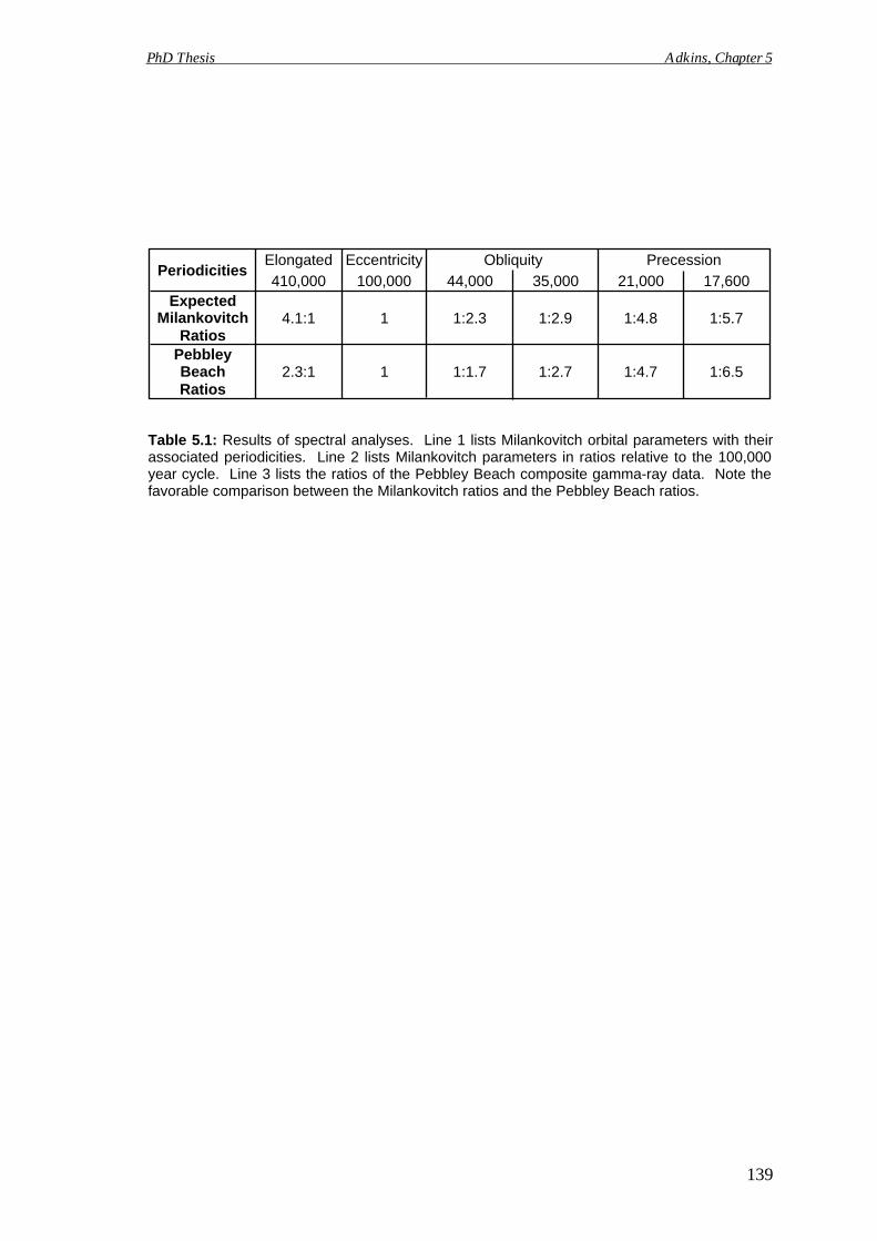
Expected
Pebbley
Obliquity44,000 35,000
Elongated410,000
Eccentricity100,000
Precession21,000 17,600
4.1:1 1 1:2.3 1:2.9 1:4.8 1:5.7
1:6.51:4.71:2.71:1.712.3:1
Periodicities
Table 5.1: Results of spectral analyses. Line 1 lists Milankovitch orbital parameters with theirassociated periodicities. Line 2 lists Milankovitch parameters in ratios relative to the 100,000year cycle. Line 3 lists the ratios of the Pebbley Beach composite gamma-ray data. Note thefavorable comparison between the Milankovitch ratios and the Pebbley Beach ratios.
PhD Thesis Adkins, Chapter 5
139
BeachRatios
RatiosMilankovitch
PhD Thesis Adkins, Chapter 5
Additionally, the spectral analyses may have been influenced by variations in
lithology. For example, in Figure 5.7 the top of column A (marked by *) is siltier than
its correlative in column C (also marked by *). Not only are these two intervals
lithologically different, they also have distinctly different gamma-ray readings.
Therefore, the spectral results could vary depending on how the individual gamma-ray
logs (Figures 5.3-5.6) are pieced together to form the composite gamma-ray log (Figure
5.8).
Another consideration is incomplete preservation of the original deposits. Major
scour surfaces occur throughout the Shoalhaven Group. As has been discussed, one of
these erosional surfaces occurs in the measured section of the Pebbley Beach
Formation. Regardless of the mechanism of formation for this scour, it most certainly
removed some of the original sediments. Although efforts have been made to present
the most complete composite section possible (Figure 5.8), it is likely that some original
deposits are missing.
Fortunately, it would be expected that the above factors would mask cyclicity,
not enhance it. Therefore, the results of the spectral analyses, combined with the
sediments' shallow-marine depositional setting, support the theory that an orbitally-
forced, glacio-eustatic driving mechanism is largely responsible for the formation of
cyclicity in the Pebbley Beach Formation.
CLIMATIC SIGNIFICANCE
This paper demonstrates that the Pebbley Beach Formation not only contains
sediments deposited by floating ice, but also records glacio-eustatic sea-level
fluctuations. Based upon paleocurrent data, Eyles et al. (1997, 1998) proposed that the
icebergs in the Permian Sydney Basin probably calved from unstable ice margins in
Antarctica. If this interpretation is correct and the ages used in Veevers' timescale
(2000b) are accurate, Gondwanan glaciation must have persisted into at least the
Ufimian stage of the Late Permian.
CONCLUSIONS
Excellent coastal exposures have allowed for detailed measurements and facies
interpretations of the Pebbley Beach Formation. Eight vertically stacked, coarsening-
and shallowing-upward cycles have been identified in outcrop. Spectral analysis has
been used to better define cyclicity in the Pebbley Beach Formation. Identified cycles
140
PhD Thesis Adkins, Chapter 5
are consistent with known mid-Permian orbital periodicities. Although depositional
cyclicity has been previously recognized in the Shoalhaven Group, this is the first study
to demonstrate a quantitative correlation between this cyclicity and the known mid-
Permian orbital parameters.
A recently published timescale based upon SHRIMP zircon dating from the
eastern coast of Australia (Veevers, 2000b) was used to date these deposits. This
timescale indicates that the Pebbley Beach Formation may be slightly younger than
previously believed. If the proposed ages are correct, the Shoalhaven Group provides
evidence that Permo-Carboniferous glaciation extended into the Late Permian.
Therefore, these deposits may record some of the final stages of Gondwanan glaciation.
141
PhD Thesis Adkins, Concluding Remarks
Concluding Remarks
PhD Thesis Adkins, Concluding Remarks
143
MAJOR CONCLUSIONS
The purpose of this project was to test for mid- to Late Permian (post-
Sakmarian) glacio-eustatic cyclothem development within Australia. This study
focuses on the largely unstudied Artinskian Tuckfield Member of the Poole Sandstone
(Fitzroy Trough, onshore Canning Basin). Data presented in this thesis demonstrate
that the cyclicity which occurs in both shallow-marine and non-marine Tuckfield
Member sequences compares favorably with the known mid-Permian earth orbital
periodicities of elongated eccentricity, eccentricity, obliquity, and precession (Chapters
2 and 3). This study also demonstrates that the Tuckfield Member cycles (i) are
laterally extensive and (ii) compare favorably with correlative shallow-marine cycles
from eastern Australia (Artinskian to Ufimian Pebbley Beach Formation, southern
Sydney Basin, New South Wales) (Chapters 2 and 5) and elsewhere in the world
(Chapter 2). The laterally extensive nature of the Tuckfield Member cycles, combined
with their strong correlation to the orbital periodicities and other correlative shallow-
marine cycles, indicate that glacio-eustatic sea-level fluctuation probably controlled the
formation of depositional cyclicity in the Fitzroy Trough during the Artinskian.
Therefore, glaciers must have persisted on Gondwana, or elsewhere, into at least the
Artinskian stage of the Early Permian, and probably into the Ufimian stage of the Late
Permian as indicated by the New South Wales deposits.
FUTURE WORK
This manuscript provides a comprehensive summary of Artinskian cyclothem
development in the onshore Canning Basin, Western Australia. It also provides a brief
summary of correlative Artinskian to Ufimian cyclothem development in the southern
Sydney Basin, New South Wales. However, it is important to remember that the work
discussed in this thesis is only a part of the larger, Australia-wide study initiated by Dr.
Steve Abbott. Similar work completed in the Carnarvon Basin has been summarized in
several manuscripts (Lever, 2002, 2003a, 2003b) and in an unpublished Ph.D. thesis
(Lever 2003c). Similar work in the Tasmanian Basin is currently in progress.
Once research from the Tasmanian Basin is complete, data from all four areas
(Canning, Carnarvon, Sydney, and Tasmanian Basins) can be compared and
synthesized into one comprehensive dataset. From this Australia-wide data, it may be
possible to develop an estimated eustatic sea-level curve for the Permian system of
Australia. This localized curve will add further support for the still contentious theory
PhD Thesis Adkins, Concluding Remarks
144
of global sea-level fluctuation. In additon, it may help refine existing Late Paleozoic
3rd-order sea-level charts (e.g. Ross and Ross, 1985, 1987). This data could be
significant because the present Permian eustacy charts are predominantly based upon
stable cratonic successions in North America (Ross and Ross, 1995). Ross and Ross
(1995) themselves recognized the importance of the Permian successions in Australia
when they wrote: "…Australia has marine and glacial-marine depositional sequences
that may eventually help tie sea-level events in high and middle latitudes of Gondwana
with those of low latitudes of cratonic North America and the Tethys."
In addition to refining global sea-level charts, the comprehensive dataset may
also be used to track the waxing and waning of glaciers and the presence of high-
latitude continental ice throughout the Permian. Since much uncertainty still surrounds
the timing of glaciation(s) and the frequency of interglacial episodes during the Permo-
Carboniferous, this could be a significant scientific contribution. Crowell (1995)
suggested that the Carboniferous and earliest Permian was marked by at least 3 distinct
episodes of glaciation. Similarly, Dickens (1996) provides convincing evidence that the
mid- to Late Permian (post-Sakmarian) was marked by alternating phases of warmer
and colder climate. Although Dickens (1996) suggests that glaciation had completely
ceased by the end of the Sakmarian, some earlier studies indicate that glaciation may
have persisted past this point (e.g. Crowell, 1995; Read, 1995). Work in the Canning
Basin suggests that glaciation did indeed continue into the Artinskian stage of the Early
Permian. Likewise, work in the Carnarvon Basin suggests that glaciers were present, at
least at high-latitudes, during the Kungurian to Ufimian stages (Lever, 2003a).
However, neither independent study can alone answer the question of whether or not
glacioeustacy consistently affected sedimentation from the Artinskian through the
Ufimian and beyond. Therefore, the major questions that remain to be answered are: (i)
Did glaciation continuously drive high-frequency, Milankovitch-band, sea-level
fluctuation throughout the Permian or are glacio-eustatic sea-level fluctuations confined
to the colder climatic periods defined by Dickens? (ii) In either case, do Milankovitch-
band, glacio-eustatic sea-level fluctuations persist up to the Triassic boundary and
beyond or do they end sometime during the Late Permian? By comparing cyclothem
development in the four temporally overlapping successions studied in this Australia-
wide project, it may be possible to answer these questions in the near future.

References
PhD Thesis Adkins, References
REFERENCES
Abbott, S.T. and Carter, R.M. (1994) The sequence architecture of mid-Pleistocene(c.1.1-0.4 Ma) cyclothems from New Zealand: facies development during aperiod of orbital control on sea-level cyclicity. In: Orbital Forcing and CyclicSequences (Eds. P.L. de Boer and D.G. Smith), Special Publication of theInternational Association of Sedimentologist, 19, 367-394.
Adkins, R.M. (2003) Regressive systems tract cyclicity in shore-zone deposits:sedimentology and stratigraphy of the Lower Permian Tuckfield Member (PooleSandstone), onshore Canning Basin, Western Australia. Australian Journal ofEarth Sciences, 50, in press.
Algeo, T.J. and Wilkinson, B.H. (1988) Periodicity of mesoscale Phanerozoicsedimentary cycles and the role of Milankovitch orbital modulation. Journal ofGeology, 96, 313-322.
Allen, J.R.L. (1964) Studies in fluviatile sedimentation: six cyclothems from the LowerOld Red Sandstone, Anglo-Welsh Basin. Sedimentology, 3, 163-198.
Apak, S.N. (1996) Depositional history of the Lower Permian Carolyn Formation andPoole Sandstone in the northern Canning Basin: implications for hydrocarbonpotential. Geological Survey of Western Australia Record 1996/8.
Apak, S.N. and Backhouse, J. (1998) Redefinition of the Grant Group andreinterpretation of the Permo-Carboniferous Succession, Canning Basin,Western Australia. In: The Sedimentary Basins of Western Australia:Proceedings of the Petroleum Exploration Society of Australia Symposium (Eds.P.G. Purcell and R.R. Purcell), 683-694.
Apak, S.N. and Carlsen, G.M. (1996) A compilation and review of data pertaining tothe hydrocarbon prospectivity in the Canning Basin. Western AustraliaGeological Survey Record 1996/10.
Astin, T.R. (1990) The Devonian lacustrine sediments of Orkney, Scotland:implications for climate cyclicity, basin structure and maturation history.Journal of the Geological Society of London, 147, 141-151.
Barrell, J. (1913) The Upper Devonian delta of the Appalachian geocyncline. AmericanJournal of Science, 36, p. 429-472.
Battersby, D.G. (1981) New Discoveries in the Surat/Bowen Basin. The APEA Journal,21, 39-44.
Bentley, J. (1984) Petroleum geology of the central Broome Platform. In: The CanningBasin W.A.: Proceedings of the Geological Society of Australia/PetroleumExploration Society of Australia Symposium (Ed. P.G. Purcell), 157-168.
Berger, A. (1977) Long-term variations of the Earth's orbital elements. CelestialMechanics, 15, 53-74.
146
PhD Thesis Adkins, References
Berger, A. (1988) Milankovitch theory and climate. Review of Geophysics, 26, 624-657.
Berger, A. and Loutre, M.F. (1994) Astronomical forcing through geological time. In:Orbital Forcing and Cyclic Sequences (Eds. P.L. de Boer and D.G. Smith),Special Publication of the International Association of Sedimentologists, 19,15-24.
Blackman, R.B. and Tukey, J.W. (1958) The measurement of power spectra from thepoint of view of communication engineering, Dover Publications, New York,190 pp.
Boardman, D.R. and Heckel, P.H. (1989) Glacial-eustatic sea-level curve for early LatePennsylvanian sequence in north-central Texas and biostratigraphic correlationwith curve for midcontinent North America. Geology, 17, 802-805.
Borer, J.M. and Harris, P.M. (1991) Lithofacies and cyclicity of the Yates Formation,Permian Basin: Implications for Reservoir Heterogeneity. American Associationof Petroleum Geologists Bulletin, 75(4), 726-779.
Botten, P. (1984) Uranium exploration in the Canning Basin: A case study. In: TheCanning Basin W.A.: Proceedings of the Geological Society ofAustralia/Petroleum Exploration Society of Australia Symposium (Ed. P.G.Purcell), 485-501.
Brakel, A.T. and Totterdell, J.M. (1993) The Sakmarian-Kungurian palaeogeography ofAustralia. In: Gondwana Eight: Assembly, Evolution, and Dispersal (Eds. R.H.Findlay, R. Unrug, M.R. Banks, and J.J. Veevers), Proceedings of the eighthGondwana symposium, pp. 385-396. Balkema, Rotterdam.
Brown, S.A., Boserio, I.M., Jackson, K.S., and Spence, K.W. (1984) The geologicalevolution of the Canning Basin-Implications for petroleum exploration. In: TheSedimentary Basins of Western Australia: Proceedings of the PetroleumExploration Society of Australia Symposium (Eds. P.G. Purcell and R.R.Purcell), 85-96.
Brown, D.A., Cambell, K.S.W., and Crook, K.A. (1968) The Geological Evolution ofAustralia and New Zealand. Pergamon Press, Oxford, 409 pp.
Bush, R.M.Q. and Rollins, H.B. (1984) Correlation of Carboniferous strata using ahierarchy of transgressive-regressive units. Geology, 12, 471-474.
Cant, D.J. (1992) Subsurface facies analysis. In: Facies Models: Response to Sea LevelChange (Eds. R.G. Walker and N.P. James), pp. 27-45. Geological Associationof Canada, St. Johns, Newfoundland.
Carey, J. (1978) Sedimentary environments and trace fossils of the Permian SnapperPoint Formation, southern Sydney Basin. Journal of the Geologocal Society ofAustralia, 25, 433-458.
147
PhD Thesis Adkins, References
Carr, P.F., Jones, B.G., and Middleton, R.G. (1989) Precursor and formation ofglendonites in the Sydney Basin. Australian Mineralogist, 4, 3-12.
Carter, R.M., Abbott, S.T. and Naish, T.R. (1999) Plio-Pleistocene cyclothems fromWanganui Basin, New Zealand: type locality for an astrochronologic time-scale,or template for recognizing ancient glacio-eustacy? Philosophical Transactionsof the Royal Society, London, 357, 1861-1872.
Carter, R.M. and Naish, T.R. (1998) A review of Wanganui Basin New Zealand: globalreference section for shallow marine, Plio-Pleistocene (2.5-0 Ma)cyclostratigraphy. Sedimentary Geology, 122, 37-52.
Clemmensen, L.B., Øxnevad, I.E.I., and De Boer, P.L. (1994) Climatic controls onancient desert sedimentation: some late Palaeozoic and Mesozoic examples fromNW Europe and the Western Interior of the USA. In: Orbital Forcing andCyclic Sequences (Eds. P.L. de Boer and D.G. Smith), Special Publication of theInternational Association of Sedimentologist, 19, 439-457.
Connolly, W.M. and Stanton, R.J. (1992) Interbasinal cyclostratigraphic correlation ofMilankovitch band transgressive-regressive cycles: Correlation ofDesmoinesian-Missourian strata between southeastern Arizona and themidcontinent of North America. Geology, 20, 999-1002.
Crowe, R.W.A. and Towner, R.R. (1976a) Permian stratigraphic nomenclature,Noonkanbah 1:250,000 sheet. Geological Survey of Western Australia, AnnualReport for 1975, 56-58.
Crowe, R.W.A. and Towner, R.R. (1976b) Environmental interpretation of the PermianNura Nura Member of the Poole Sandstone, Noonkanbah Sheet Area, CanningBasin: A gradation between fluviatile and shallow-water marine facies.Geological Survey of Western Australia, Annual Report for 1975, 59-62.
Crowe, R.W.A. and Towner, R.R. (1977) Definitions of some new and revised rockunits in the Canning Basin. Geological Survey of Western Australia, Record1976/24.
Crowe, R.W.A. and Towner, R.R. (1981) Noonkanbah, Western Australia: 1:250,000Geological Series-Explanatory Notes. Australian Government PublishingService, Canberra.
Crowell, J.C. (1975) The Late Paleozoic glaciation. In: Gondwana Geology (Ed.K.S.W. Campbell), pp. 313-331. Australian National University Press,Canberra.
Crowell, J.C. (1978) Gondwanan glaciation, cyclothems, continental positioning, andclimate change. American Journal of Science, 278, 1345-1372.
148
PhD Thesis Adkins, References
Crowell, J.C. (1995) The ending of the Late Paleozoic Ice Age during the PermianPeriod. In: The Permian of Northern Pangea, v. 1, Paleogeography,Paleoclimates, Stratigraphy (Eds. P.A. Scholle, T.M. Peryt and D.S. Ulmer-Scholle), pp. 62-74. Springer-Verlag, Berlin.
Crowell, J.C. and Frakes, L.A. (1971) Late Paleozoic Glaciation: Part IV, Australia.Geological Society of America Bulletin, 82, 2515-2540.
De Boer, P.L. and Smith, D.G. (1994) Orbital forcing and cyclic sequences. In: OrbitalForcing and Cyclic Sequences (Eds. P.L. de Boer and D.G. Smith), SpecialPublication of the International Association of Sedimentologists, 19, 1-14.
Dickens, J.M. (1985) Late Palaeozoic glaciation. BMR Journal of Australian Geologyand Geophysics, 9, 163-169.
Dickens, J.M. (1996) Problems of a Late Palaeozoic glaciation in Australia andsubsequent climate in the Permian. Palaeogeography, Palaeoclimatology,Palaeoecology, 125, 185-197.
Eden, D.J. and Eyles, N. (2001) Description and numerical model of Pleistoceneiceberg scours and ice-keel turbated facies at Toronto, Canada. Sedimentology,48, 1079-1102.
Ellyard, E.J. (1984) Oil migration in the northern Canning Basin-A regional review. In:The Canning Basin W.A.: Proceedings of the Geological Society ofAustralia/Petroleum Exploration Society of Australia Symposium (Ed. P.G.Purcell), 359-376.
Eyles, C.H. and Eyles, N. (2000) Subaqueous mass flow origin for Lower Permiandiamictites and associated facies of the Grant Group, Barbwire Terrace, CanningBasin, Western Australia. Sedimentology, 47, 343-356.
Eyles, C.H., Eyles, N., and Gostin, V.A., (1998) Facies and allostratigraphy of highlatitude, glacially influenced marine strata of the Early Permian southern SydneyBasin, Australia. Sedimentology, 45, 121-161.
Eyles, C.H., Mory, A.J., and Eyles, N. (2003) Carboniferous-Permian facies andtectonostratigraphic successions of the glacially influenced and rifted CarnarvonBasin, western Australia. Sedimentary Geology, 155, 63-86.
Eyles, N., Eyles, C.H., Apak, S.N., and Carlsen, G.M. (2001) Permian-Carboniferoustectono-stratigraphic evolution and petroleum potential of the northern CanningBasin, Western Australia. American Association of Petroleum GeologistsBulletin, 85(6), 989-1006.
Eyles, N., Eyles, C.H., and Gostin, V.A. (1997) Iceberg rafting and scouring in theEarly Permian Shoalhaven Group of New South Wales, Australia: Evidence ofHeinrich-like events? Palaeogeography, Palaeoclimatology, Palaeoecology,136, 1-17.
149
PhD Thesis Adkins, References
Eyles, N., Mory, A.J., and Backhouse, J. (2002) Carboniferous-Permianpalynostratigraphy of west Australian marine rift basins: resolving tectonic andeustatic controls during Gondwanan glaciations. Palaeogeography,Palaeoclimatology, Palaeoecology, 184, 305-319.
Fielding, C.R. and Webb, J.A. (1996) Facies and cyclicity of the Late PermianBainmedart Coal Measures in the northern Prince Charles Mountains,MacRobertson Land, Antarctica. Sedimentology, 43, 295-322.
Frakes, L.A. (1969) Late Paleozoic glaciation: pt 1: South America. Geological Societyof America Bulletin, 80, 1007-1042.
Galloway, W.E. and Hobday, D.K. (1996) Terrigenous Clastic Depositional Systems:Applications to Fossil Fuel and Groundwater Resources, 2nd edition, Springer,Berlin, 489 pp.
Gibson, D. L. (1983) Pender, Western Australia: 1:250,000 Geological Series-Explanatory Notes. Australian Government Publishing Service, Canberra.
Gibson, D.L. and Crowe, R.W.A. (1982) Mount Anderson (2nd edition), WesternAustralia: 1:250,000 Geological Series-Explanatory Notes. AustralianGovernment Publishing Service, Canberra.
Goldhammer, R.K., Oswald, E.J., and Dunn, P.A. (1994) High-frequency glacio-eustatic cyclicity in the Middle Pennsylvanian of the Paradox Basin: anevaluation of Milankovitch forcing. In: Orbital Forcing and Cyclic Sequences(Eds. P.L. de Boer and D.G. Smith), Special Publication of the InternationalAssociation of Sedimentologists, 19, 243-283.
Goldstein, B.A. (1989) Waxings and wanings in stratigraphy, play concepts, andprospectivity in the Canning Basin. The APEA Journal, 29(1), 466-508
Gonzalez-Bonorino, G. and Eyles, N. (1995) Inverse relationship between ice extentand the late Paleozoic glacial record of Gondwana. Geology, 23, 1015-1018.
Gostin, V.A. and Herbert, C. (1973) Stratigraphy of the Upper Carboniferous andLower Permian sequence, southern Sydney Basin. Journal of the GeologicalSociety of Australia, 20, 49-70.
Griffin, T.J., Tyler, I.M., and Playford, P.E. (1993) Lennard River (3rd Edition),Western Australia: 1:250,000 Geological Series-Explanatory Notes. Perth.
Guppy, D.J., Lindner, A.W., Rattigan, J.J., and Casey, J.N. (1952) The stratigraphy ofthe Mesozoic and Permian sediments of the Desert Basin, Western Australia.19th International Geological Congress (Gondwana Symposium) Algeria, 101-114.
Guppy, D.J., Lindner, A.W., Rattigan, J.J., and Casey, J.N. (1958) The geology of theFitzroy Basin, Western Australia. Bureau of Mineral Resources, Australia,Bulletin 36.
150
PhD Thesis Adkins, References
Hambrey, M.J. and Harland, W.B. (1981) Earth's pre-Pleistocene glacial record,Cambridge University Press, Cambridge, 1004 pp.
Haq, B.U., Hardenbol, J., and Vail, P.R. (1987) Chronology of fluctuating sea levelssince the Triassic. Science, 235, 1156-1167.
Havord, P., Apak, S.N., and Carlsen, G.M. (1997) Permo-Carboniferous petroleumreservoir data, selected wells, Canning Basin, Western Australia. GeologicalSurvey of Western Australia Record 1996/11.
Haykin, S. (1983) Nonlinear methods of spectral analysis, 2nd edition, Springer-Verlag,Berlin.
Hays, J.D., Imbrie, J., and Shackleton, N.J. (1976) Variations in the Earth's orbit:Pacemaker of the ice ages. Science, 194, 1121-1132.
Heckel, P.H. (1977) Origin of phosphatic black shale facies in Pennsylvaniancyclothems of mid-continent North America. American Association ofPetroleum Geologists Bulletin, 61, 1045-1068.
Heckel, P.H. (1986) Sea-level curve for Pennsylvanian eustatic marine transgressive-regressive depositional cycles along midcontinent outcrop belt, North America.Geology, 14, 330-334.
Herbert, C. (1980a) Southwestern Sydney Basin. Geological Survey of New SouthWales Bulletin, 26, 10-52.
Herbert, C. (1980b) Evidence for Glaciation in the Sydney Basin and Tamworthsynclinorial zone. Geological Survey of New South Wales Bulletin, 26, 274-293.
Hinnov, L.A. (2000) New Perspectives on Orbitally Forced Stratigraphy. AnnualReview of Earth and Planetary Sciences, 28, 419-475.
Hocking, R., Mory, A.J., and Williams, I.R. (1994) An atlas of Neoproterozoic andPhanerozoic Basins of Western Australia. In: The Sedimentary Basins ofWestern Australia: Proceedings of thePetroleum Exploration Society ofAustralia Symposium (Eds. P.G. Purcell and R.R. Purcell), 21-43.
Horstman, E.L. (1984) Source rocks in the Canning Basin: A review. In: The CanningBasin W.A.: Proceedings of the Geological Society of Australia/PetroleumExploration Society of Australia Symposium (Ed. P.G. Purcell), 345-352.
House, M.R. (1995) Orbital forcing timescales: an introduction. In: Orbital ForcingTimescales and Cyclostratigraphy (Eds. M.R. House and A.S. Gale), GeologicalSociety Special Publication, 85, 1-18.
Hunt, D. and Tucker, M.E. (1992) Stranded parasequences and the forced regressivewedge systems tract: deposition during base-level fall. Sedimentary Geology, 81,1-9.
151
PhD Thesis Adkins, References
Imbrie, J. (1985) A theoretical framework for the Pleistocene ice ages. Journal of theGeological Society, London, 142, 417-432.
Imbrie, J. and Imbrie, K.P. (1979) Ice Ages: Solving the Mystery. Enslow Publishing,Short Hills, NJ.
Jackson, M.J., Kennard, J.M., Romine, K., Southgate, P.N., Jones, P.J., Nicoll, R.,Young, G., and Zeilinger, I. (1994) Petroleum systems in the Canning Basin.The APEA Journal, 34(1), 142-155.
Kennard, J.M., Jackson, M.J., Romine, K.K., Shaw, R.D., and Southgate, P.N. (1994)Depositional sequences and associated petroleum systems of the Canning Basin,WA. In: The Sedimentary Basins of Western Australia: Proceedings ofthePetroleum Exploration Society of Australia Symposium (Eds. P.G. Purcelland R.R. Purcell), 657-676.
Klein, G. deV. and Willard, D.A. (1989) Origin of the Pennsylvanian coal-bearingcyclothems of North America. Geology, 17, 152-155.
Lambeck, K (1980) The Earth's Variable Rotation: its Origin, History, and PhysicalConstitution (6th edition). Cambridge University Press, Cambridge.
Lever, H. (2002) Stratigraphy of the Upper Permian Kennedy Group of the onshoreCarnarvon Basin (Merlinleigh Sub-basin), Western Australia. AustralianJournal of Earth Sciences, 49 (3), 539-550.
Lever, H. (2003a) Cyclic sedimentation in the shallow marine Late Permian KennedyGroup, Carnarvon Basin, Western Australia. Submitted to Sedimentary Geology.
Lever, H. (2003b) Climatic belts in the mid-Late Permian: evidence from the KennedyGroup, onshore Carnarvon Basin, Western Australia. Submitted to Gondwana11.
Lever, H. (2003c) Cyclicity in the Late Permian Kennedy Group, Carnarvon Basin,Western Australia: causes of cyclic sedimentation in a shallow marine sea.Unpublished Ph.D. thesis. James Cook University, Townsville.
Miall, A.D. (1997) The Geology of Stratigraphic Sequences. Springer-Verlag, Berlinand Heidelberg, 433 pp.
Michaelsen, P. and Henderson, R.A. (2000) Facies relationships and cyclicity of highlatitude, Late Permian coal measures, Bowen Basin, Australia. InternationalJournal of Coal Geology, 44, 19-48.
Middleton, M.F. (1992) Seismic Stratigraphy, Structural Analysis, and TectonicEvolution of the Northern Canning Basin, Western Australia. Geological Surveyof Western Australia Record 1991/5.
152
PhD Thesis Adkins, References
Miller, D.J. and Eriksson, K.A. (2000) Sequence stratigraphy of Upper Mississippianstrata in the central Appalachians: A record of glacioeustasy and tectonoeustasyin a foreland basin setting. American Association of Petroleum GeologistsBulletin, 84, 210-233.
Naish, T., Beu, A.G., Carter, R.M., Edwards, A.R., Kamp, P.J.J., Pilans, B., Saul, G.,and Wolf, K. (1998) Astronomical calibration of a Southern Hemisphere Plio-Pleistocene reference section, Wanganui Basin, New Zealand. QuaternaryScience Review, 17, 695-710.
Naish, T. and Kamp, P.J.J. (1997) Sequence stratigraphy of sixth-order (41 k.y.)Pliocene Pleistocene cyclothems, Wanganui Basin, New Zealand: A case for theregressive systems tract. Geological Society of America Bulletin, 109(8), 978-999.
Nicoll, R.S. (1984) Conodont studies in the Canning Basin-A review and update. In:The Canning Basin W.A.: Proceedings of the Geological Society ofAustralia/Petroleum Exploration Society of Australia Symposium (Ed. P.G.Purcell), 439-444.
O'Brien, P.E., Lindsey, J.F., Knauer, K., and Sexton, M.J. (1998) Sequence stratigraphyof a sandstone-rich Permian glacial succession, Fitzroy Trough, Canning Basin,Western Australia. Australian Journal of Earth Sciences, 45, 533-545.
Olsen, H. (1990) Astronomical forcing of meandering river behavior: Milankovitchcycles in Devonian of East Greenland. Palaeogeography, Palaeoclimatology,Palaeoecology, 79, 99-115.
Olsen, H. (1994) Orbital forcing on continental depositional systems–lacustrine andfluvial cyclicity in the Devonian of East Greenland. In: Orbital Forcing andCyclic Sequences (Eds. P.L. de Boer and D.G. Smith), Special Publication of theInternational Association of Sedimentologist, 19, 429-438.
Olsen, P.E. (1986) A 40-million-year lake record of early Mosozoic orbital climaticforcing. Science, 234, 842-848.
Olsen, P.E. and Kent, D.V. (1999) Long-period Milankovitch cycles from the LateTriassic and Early Jurassic of eastern North America and their implications forthe calibration of the Early Mesozoic time-scale and the long-term behavior ofthe planets. Philosophical Transactions of the Royal Society, London, 357,1761-1786.
Paillard, D., Labeyrie, L., and Yiou, P. (1996) Macintosh Program Performs Time-Series Analysis. www.agu.org/eos_elec.
Payton, C. E. (Ed.) (1977) Seismic Stratigraphy – Applications to HydrocarbonExploration. American Association of Petroleum Geologists, Memoir 26, 516 p.
153
PhD Thesis Adkins, References
Playford, P.E. (1984) Platform-margin and marginal-slope relationships in Devonianreef complexes of the Canning Basin. In: The Canning Basin W.A.: Proceedingsof the Geological Society of Australia/Petroleum Exploration Society ofAustralia Symposium (Ed. P.G. Purcell), 189-214.
Plint, A.G. (1988) Global eustacy and the Eocene sequence in the Hampshire Basin,England. Basin Research, 1, 11-22.
Posamentier, H.W., Allen, G.P., James, D.P., Tesson, M. (1992) Forced regressions in asequence stratigraphic framework: concepts, examples, and explorationsignificance. Bulletin of the American Association of Petroleum Geologists, 76,1687-1709.
Purcell, P.G. (1984) The Canning Basin, W.A. - An Introduction. In: The CanningBasin WA: Proceedings of the Geological Society of Australia/PetroleumExploration Society of Australia Symposium (Ed. P.G. Purcell), 3-19.
Purcell, P.G. and Poll, J. (1984) The Seismic Definition of the Main Structural Elementsof the Canning Basin. In: The Canning Basin WA: Proceedings of theGeological Society of Australia/Petroleum Exploration Society of AustraliaSymposium (Ed. P.G. Purcell), 73-84.
Purcell, P.G. and Purcell, R.R. (1994) The Sedimentary Basins of Western Australia:Proceedings of the Petroleum Exploration Society of Australia Symposium.
Rampino, M.R., Prokoph, A., and Adler, A. (2000) Tempo of the end-Permian event:High resolution cyclostratigraphy at the Permian-Triassic boundary. Geology,28, 643-646.
Ramsbottom, W.H.C. (1979) Rates of transgression and regression in the Carboniferousof NW Europe. Journal of the Geological Society, London, 136, 147-153.
Read, J.F. (1995) Overview of carbonate platform sequences, cycle stratigraphy andreservoirs in greenhouse and ice-house worlds. In: Milankovitch Sea LevelChanges, Cycles and Reservoirs on Carbonate Platforms in Greenhouse andIce-house Worlds (Eds. J.F. Read, C. Kerans, and L.J. Weber) SEPM ShortCourse Notes, 35, Part 1, 102 pp.
Redfern, J. and Millward, E. (1994) A review of the sedimentology and stratigraphy ofthe Permo Carboniferous Grant Group, Canning Basin, Western Australia. In:The Sedimentary Basins of Western Australia: Proceedings of the PetroleumExploration Society of Australia Symposium (Eds. P.G. Purcell and R.R.Purcell), 753-756.
Reijmer, J.J.G., Sprenger, A., Ten Kate, W.G.H.Z., Schlager, W., and Krystyn, L.(1994) Periodicities in the composition of Late Triassic calciturbidites (EasternAlps, Austria). In: Orbital Forcing and Cyclic Sequences (Eds. P.L. de Boerand D.G. Smith), Special Publication of the International Association ofSedimentologists, 19, 323-343.
154

PhD Thesis Adkins, References
Roberts, J., Claoue-Long, J., and Foster, C.B. (1996) SHRIMP zircon dating of thePermian System of eastern Australia. Australian Journal of Earth Sciences, 43,401-421.
Ross, C.A. and Ross, J.R.P. (1985) Late Paleozoic depositional sequences aresynchronous and worldwide. Geology, 13, 194-197.
Ross, C.A. and Ross, J.R.P. (1988) Late Paleozoic trangressive-regressive deposition.In: Sea-level changes: An intergrated approach: Society of EconomicPaleontologists and Mineralogists Special Publication 42 (Eds. C.K. Wilgus,B.S. Hastings, C.G. St. C. Kendall, H.W. Posamentier, C.A. Ross, and J.C. VanWagoner), 228-247.
Ross, C.A. and Ross, J.R.P. (1987) Late Paleozoic sea levels and depositionalsequences. In: Timing and Depositional History of Eustatic Sequences:Constraints of Seismic Stratigraphy (Eds. C.A. Ross and D. Haman), SpecialPublication 124, pp 137-149. Cushman Foundation for Foraminiferal Research,Ithaca.
Ross, C.A. and Ross, J.R.P. (1995) Permian Sequence Stratigraphy. In: The Permian ofNorthern Pangea, v. 1, Paleogeography, Paleoclimates, Stratigraphy (Eds. P.A.Scholle, T.M. Peryt and D.S. Ulmer-Scholle), pp. 98-123. Springer-Verlag,Berlin.
Runnegar, B.N. (1979) Ecology of Eurydesma and the Eurydesma fauna, Permian ofeastern Australia. Alcheringa, 3, 261-285.
Runnegar, B.N. (1980) Excursion Guide, Day 7, Stop 3, Montague Roadstead, JervisBay (Early Permian Shoalhaven Group), New South Wales Geological SurveyBulletin, 26, 523-530.
Santos, P.R. dos, Rocha-Compos, A.C., and Canuto, J.R. (1996) Patterns of latePaleozoic deglaciation in the Parana Basin, Brazil. Palaeogeography,Palaeoclimatology, Palaeoecology, 125, 941-163.
Saul, G., Naish, T.R., Abbott, S.T., and Carter, R.M. (1999) Sedimentary cyclicity inthe marine Plio-Pleistocene of the Wanganui basin (New Zealand): Sequencestratigraphic motifs characteristic of the past 2.5 m.y. Geological Society ofAmerica Bulletin, 111(4), 524-537.
Scheibner, E. (1974) A plate tectonic model of the Paleozoic tectonic history of NewSouth Wales. Journal of the Geologcial Society of Australia, 20, 405-426.
Scheibner, E. and Basden, H. (1998) Geology of New South Wales-Synthesis. Volume2 Geological Evolution. New South Wales Geological Survey Memoirs, 13, 666pp.
Schwarzacher, W. (1993) Cyclostratigraphy and the Milankovitch Theory,Developments in Sedimentology 52, Elsevier, Amsterdam, 225 pp.
155
PhD Thesis Adkins, References
Scotese, C.R., Boucot, A.J., and McKerrow, W.S. (1999) Gondwanan palaeogeographyand palaeoclimatology. Journal of African Earth Sciences 28(1), 99-114.
Shackleton, N.J. and Opdyke, N.D. (1973) Oxygen isotope and palaeo-magneticstratigraphy of Pacific core V28-238: oxygen isotope temperatures and icevolumes in a 105 and 106 year scale. Quaternary Research, 3, 39-55.
Shaw, R.D., Tyler, I.M., Griffin, T.J., and Webb, A. (1992a) New K-Ar constraints onthe onset of subsidence in the Canning Basin, Western Australia. Journal ofAustralian Geology and Geophysics, 13, 31-35.
Shaw, R.D., Zeitler, P.K., McDougall, I., and Tingate, P.R. (1992b) The Palaeozoichistory of an unusual intracratonic thrust belt in central Australia based on 40Ar-39Ar, K-Ar and fission track dating. Journal of the Geological Society, London,149, 937-954.
Sierro, F.J., Ledesma, S., Flores, J.A., Torrescusa, S., and Martinez del Olmo, W.(2000) Sonic and gamma-ray astrochronology: Cycle to cycle calibration ofAtlantic climatic records to Mediterranean sapropels and astronomicaloscillations. Geology, 28 (8), 695-698.
Smith, A.G., Hurley, A.M., and Briden, J.C. (1981) Phanerozoic PaleocontinentalWorld Maps, Cambridge University Press, London, 102 pp.
Smith, N.D. and Ashley, G. (1985) Proglacial lacustrine environment. In: Glacialsedimentary environments (Eds. G.M. Ashley, J. Shaw, and N.D. Smith),Society of Economic Paleontologists and Mineralogists Short Course, 16, 135-216.
Spaulding, W.G. (1991) Pluvial climatic episodes in North America and North Africa:types and correlation with global climate. Palaeogeography,Palaeoclimatology, Palaeoecology, 84, 217-227.
Suess, E., Balzer, W., Hess, E.K.F., Muller, P.J., and Wefer, G. (1985) Calciumcarbonate hexahydrate from organic-rich sediments of the Antarctic shelf:Precursor of glendonites. Science, 1216, 1128-1131.
Talbot, M.R. (1985) Major bounding surfaces in eolian sandstones-a climatic model.Sedimentology, 32, 257-265.
Tankard, A.J. (1986) Depostional response to foreland deformation in theCarboniferous of eastern Kentucky. American Association of PetroleumGeologists Bulletin, 70, 853-868.
Tiedemann, R., Sarnthein, M., Shackleton, N.J. (1994) Astromomical timescale for thePliocene Atlantic d18O and dust flux records of Ocean Drilling Program site 659.Paleoceanography, 9, 619-638.
156
PhD Thesis Adkins, References
Towner, R.R. (1981) Derby (2nd Edition), Western Australia: 1:250,000 GeologicalSeries-Explanatory Notes. Australian Geovernment Publishing Services,Canberra.
Tye, S.C., Fielding, C.R., and Jones, B.G. (1996) Stratigraphy and sedimentology of thePermian Talaterang and Shoalhaven Groups in the southernmost Sydney Basin,New South Wales. Australian Journal of Earth Sciences, 43, 57-69.
Udden, J.A. (1912) Geology and mineral resources of the Peoria quadrangle, Illinois.U.S. Geological Survey Bulletin 506, 47-50.
Vail, P.R., Audemard, F., Bowman, S.A., Eisner, P.N., Perez-Cruz, C. (1991) Thestratigraphic signatures of tectonics, eustasy and sedimentology – an overview.In: Cycles and Events in Stratigraphy, (Eds. G. Einsele, W. Ricken, and A.Seilacher), 617-659.
Vail, P.R., Mitchum, R.M., and Thompson, S. (1977) Seismic stratigraphy and globalchanges of sea level, part 4: global cycles of relative changes of sea level.American Association of Petroleum Geologist, Memior 26, 83-97.
Veevers, J.J. (2000a) Permian-Triassic Pangean basins and foldbelts along thePanthalassan margin of Gondwanaland. In: Billion-year earth history ofAustralia and neighbours in Gondwanaland (Ed. J.J. Veevers), pp. 292-308,Gemoc Press, Sydney.
Veevers, J.J. (2000b) Time Scale. In: Billion-year earth history of Australia andneighbours in Gondwanaland (Ed. J.J. Veevers), pp. 3-8, Gemoc Press, Sydney.
Veevers, J.J. (2000c) Australia in Pangea and Gondwanaland. In: Billion-year earthhistory of Australia and neighbours in Gondwanaland (Ed. J.J. Veevers), pp. 9-11, Gemoc Press, Sydney.
Veevers, J.J., Conaghan, P.J. and Powell, C.McA. (1994b) Eastern Australia. In:Permian Triassic basins and foldbelts along the Panthalassan margin ofGondwanaland (Eds. J.J. Veevers and C.McA. Powell), Geological Society ofAmerica Memoirs, 184, 11-171.
Veevers, J.J. and Powell, C.McA. (1987) Late Paleozoic glacial episodes inGondwanaland reflected in transgressive-regressive depositional sequences inEuramerica. Geological Society of America Bulletin, 98, 475-487.
Veevers, J.J., Powell, C.McA., Collinson, J.W., and Lopez-Gamundi, O.R. (1994a)Synthesis. In: Permian-Triassic basins and foldbelts along the Panthalassanmargin of Gondwanaland (Eds. J.J. Veevers and C.McA. Powell), GeologicalSociety of America Memoirs, 184, 331-353.
Visser, J.N.J. (1993a) Sea-level changes in a back-arc-foreland transition: the lateCarboniferous-Permian Karoo Basin of South Afric. Sedimentary Geology, 83,115-131.
157
PhD Thesis Adkins, References
Visser, J.N.J. (1993b) A reconstruction of the late Palaeozoic ice sheet on southwesternGondwana. In: Gondwana Eight: Assembly, Evolution, and Dispersal (Eds. R.H.Findlay, R. Unrug, M.R. Banks, and J.J. Veevers), Proceedings of the eighthGondwana symposium, pp. 449-458. Balkema, Rotterdam.
Visser, J.N.J. (1989) The Permo-Carboniferous Dwyka Formation of southern Africa:deposition by a predominantly subpolar marine ice sheet. Palaeogeography,Palaeoclimatology, Palaeoecology, 70, 377-391.
Visser, J.N.J. (1996) Controls on Early Permian Shelf deglaciation in the Karoo Basinof South Africa. Palaeogeography, Palaeoclimatology, Palaeoecology, 125,129-139.
Von Brun, V, (1996) The Dwyka Group in the nothern part of the Kwazulu/Natal,South Africa: sedimentation during Late Paleaeozoic deglaciation.Palaeogeography, Palaeoclimatology, Palaeoecology, 125, 941-163.
Wanless, H.R. and Shephard, F.P. (1936) Sea level and climatic changes related to LatePaleozoic cycles. Geological Society of America Bulletin, 47, 1177-1206.
Weedon, G.P. (1991) The spectral analysis of stratigraphic time series. In: Cycles andEvents in Stratigraphy (Eds. G. Einsele, W. Ricken, and A. Seilacher), pp. 840-854, Springer-Verlag, Berlin, Germany.
Weedon, G.P., Jenkyns, H.C., Coe, A.L., and Hesselbo, S.P. (1999) Astronomicalcalibration of the Jurassic time-scale from cyclostratigraphy in Britsih mudrockformations. Philosophical Transactions of the Royal Society, London, 357,1787-1813.
Weedon, G.P. and Read, W.A. (1995) Orbital-climatic forcing of Namurian cyclicsedimentation from spectral analysis of the Limestone Coal Formation, CentralScotland. In: Orbital-forcing, Timescales, and Cyclostratigraphy (Eds. M.R.House and A.S. Gale), Geological Society of London Special Publication, 85,51-66.
Weller, J.M. (1931) The conception of cyclical sedimentation during the Pennsylvanianperiod. Illinois State Geological Survey Bulletin 60, 163-177.
Wood, R. (2000) Novel paleoecology of a postextinction reef: Famennian (LateDevonian) of the Canning Basin, northwestern Australia. Geology, 28(11), 987-990.
Yeates, A.N., Crowe, R.W.A., Towner, R.R., Wyborn, L.A.I., and Passmore, V.L.(1975) Notes on the geology of the Gregory Sub-basin and adjacent areas of theCanning Basin, Western Australia. Bureau of Mineral Resoureces, Australia,Record 1975/77.
158
PhD Thesis Adkins, References
Yeates , A.N., Gibson, D.L., Towner, R.R., and Crowe, R.W.A. (1984) RegionalGeology of the Onshore Canning Basin, W.A. In: The Canning Basin W.A.:Proceedings of the Geological Society of Australia/Petroleum ExplorationSociety of Australia Symposium (Ed. P.G. Purcell), 23-55.
Zachos, J.C., Flower, B.P., and Paul, H. (1997) Orbitally placed climate oscillationsacross the Oligocene/Miocene boundary. Nature, 388, 567-570.
Zachos, J., Pagani, M, Sloan, L., Thomas, E., and Billups, K. (2001) Trends, Rhythms,and Aberrations in Global Climate 65 Ma to Present. Science, 292, 686-693.
159