midas regressions: further results and new directions∗
TRANSCRIPT

MIDAS Regressions:
Further Results and New Directions∗
Eric Ghysels† Arthur Sinko‡ Rossen Valkanov§
First Draft: February 2002
This Draft: February 7, 2006
Abstract
We explore Mixed Data Sampling (henceforth MIDAS) regression models. The regressions
involve time series data sampled at different frequencies. Volatility and related processes are
our prime focus, though the regression method has wider applications in macroeconomics and
finance, among other areas. The regressions combine recent developments regarding estimation
of volatility and a not so recent literature on distributed lag models. We study various lag
structures to parameterize parsimoniously the regressions and relate them to existing models.
We also propose several new extensions of the MIDAS framework. The paper concludes with an
empirical section where we provide further evidence and new results on the risk-return tradeoff.
We also report empirical evidence on microstructure noise and volatility forecasting.
∗We thank two Referees and an Associate Editor, Alberto Plazzi, Pedro Santa-Clara as well as seminarparticipants at City University of Hong Kong, Emory University, the Federal Reserve Board, ITAM, KoreaUniversity, New York University, Oxford University, Tsinghua University, University of Iowa, UNC, USC,participants at the Symposium on New Frontiers in Financial Volatility Modelling, Florence, the AcademiaSinica Conference on Analysis of High-Frequency Financial Data and Market Microstructure, Taipei, theCIREQ-CIRANO-MITACS conference on Financial Econometrics, Montreal and the Research TriangleConference, for helpful comments. All remaining errors are our own.
†Department of Finance, Kenan-Flagler School of Business and Department of Economics University ofNorth Carolina, Gardner Hall CB 3305,Gardner Hall CB 3305, Chapel Hill, NC 27599-3305, phone: (919)966-5325, e-mail: [email protected].
‡Department of Economics, University of North Carolina, Gardner Hall CB 3305, Chapel Hill, NC 27599-3305, e-mail: [email protected]
§Rady School of Management, UCSD, Pepper Canyon Hall, 3rd Floor 9500 Gilman Drive, MC 0093 LaJolla, CA 92093-0093, phone: (858) 534-0898, e-mail: [email protected].

1 Introduction
The availability of data sampled at different frequency always presents a dilemma for a
researcher working with time series data. On the one hand, the variables that are available
at high frequency contain potentially valuable information. On the other hand, the researcher
cannot use this high frequency information directly if some of the variables are available at
a lower frequency, because most time series regressions involve data sampled at the same
interval. The common solution in such cases is to “pre-filter” the data so that the left-hand
and right-hand side variables are available at the same frequency. In the process, a lot of
potentially useful information might be discarded, thus rendering the relation between the
variables difficult to detect.1 As an alternative, Ghysels, Santa-Clara, and Valkanov (2002),
(2004) and (2005) have recently proposed regressions that directly accommodate variables
sampled at different frequencies. Their MIxed Data Sampling – or MIDAS – regressions
represent a simple, parsimonious, and flexible class of time series models that allow the
left-hand and right-hand side variables of time series regressions to be sampled at different
frequencies.
Since MIDAS regressions have only recently been introduced, there are a lot of unexplored
questions. The goal of this paper is to explore some of the most pressing issues, to lay
out some new ideas about mixed-frequency regressions, and to present some new empirical
results. Before we start, it is useful to introduce a simple MIDAS regression. Suppose that
a variable yt is available once between t − 1 and t (say, monthly), another variable x(m)t is
observed m times in the same period (say, daily or m = 22), and that we are interested in
the dynamic relation between yt and x(m)t . In other words, we want to project the left-hand
side variable yt onto a history of lagged observations of x(m)t−j/m. The superscript on x
(m)t−j/m
denotes the higher sampling frequency and its exact timing lag is expressed as a fraction of
the unit interval between t − 1 and t. A simple MIDAS model is
yt = β0 + β1B(L1/m; θ)x(m)t + ε
(m)t (1)
for t = 1, . . . , T and where B(L1/m; θ) =∑K
k=0 B(k; θ)Lk/m and L1/m is a lag operator such
that L1/mx(m)t = x
(m)t−1/m, and the lag coefficients in B(k; θ) of the corresponding lag operator
Lk/m are parameterized as a function of a small-dimensional vector of parameters θ.
1This situation is becoming more frequent now as dramatic improvements in information gathering haveproduced new, high-frequency datasets, particularly in the area of financial econometrics.
1
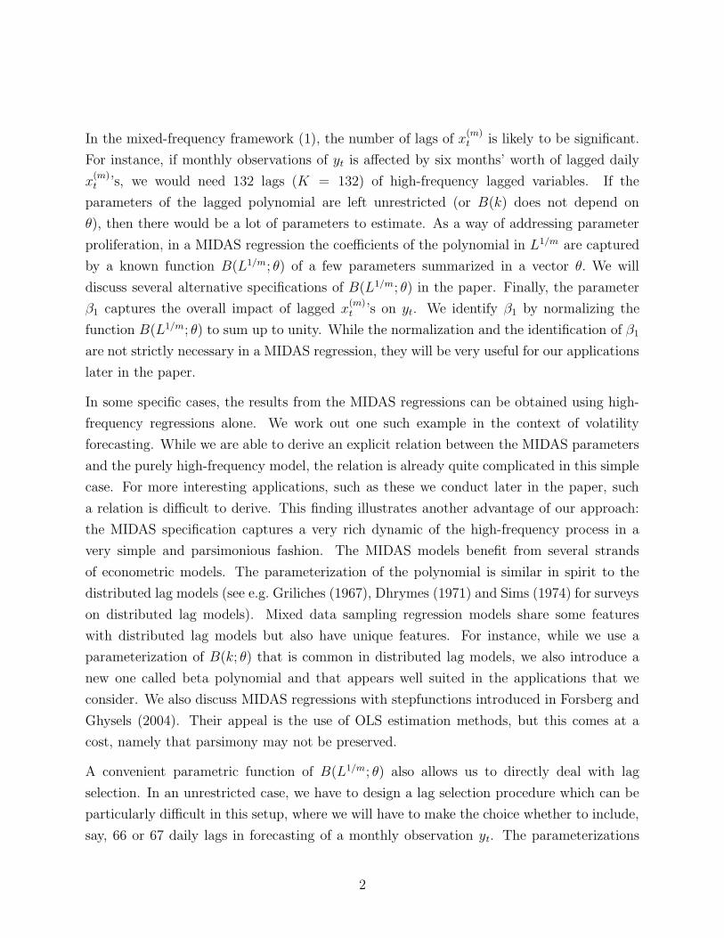
In the mixed-frequency framework (1), the number of lags of x(m)t is likely to be significant.
For instance, if monthly observations of yt is affected by six months’ worth of lagged daily
x(m)t ’s, we would need 132 lags (K = 132) of high-frequency lagged variables. If the
parameters of the lagged polynomial are left unrestricted (or B(k) does not depend on
θ), then there would be a lot of parameters to estimate. As a way of addressing parameter
proliferation, in a MIDAS regression the coefficients of the polynomial in L1/m are captured
by a known function B(L1/m; θ) of a few parameters summarized in a vector θ. We will
discuss several alternative specifications of B(L1/m; θ) in the paper. Finally, the parameter
β1 captures the overall impact of lagged x(m)t ’s on yt. We identify β1 by normalizing the
function B(L1/m; θ) to sum up to unity. While the normalization and the identification of β1
are not strictly necessary in a MIDAS regression, they will be very useful for our applications
later in the paper.
In some specific cases, the results from the MIDAS regressions can be obtained using high-
frequency regressions alone. We work out one such example in the context of volatility
forecasting. While we are able to derive an explicit relation between the MIDAS parameters
and the purely high-frequency model, the relation is already quite complicated in this simple
case. For more interesting applications, such as these we conduct later in the paper, such
a relation is difficult to derive. This finding illustrates another advantage of our approach:
the MIDAS specification captures a very rich dynamic of the high-frequency process in a
very simple and parsimonious fashion. The MIDAS models benefit from several strands
of econometric models. The parameterization of the polynomial is similar in spirit to the
distributed lag models (see e.g. Griliches (1967), Dhrymes (1971) and Sims (1974) for surveys
on distributed lag models). Mixed data sampling regression models share some features
with distributed lag models but also have unique features. For instance, while we use a
parameterization of B(k; θ) that is common in distributed lag models, we also introduce a
new one called beta polynomial and that appears well suited in the applications that we
consider. We also discuss MIDAS regressions with stepfunctions introduced in Forsberg and
Ghysels (2004). Their appeal is the use of OLS estimation methods, but this comes at a
cost, namely that parsimony may not be preserved.
A convenient parametric function of B(L1/m; θ) also allows us to directly deal with lag
selection. In an unrestricted case, we have to design a lag selection procedure which can be
particularly difficult in this setup, where we will have to make the choice whether to include,
say, 66 or 67 daily lags in forecasting of a monthly observation yt. The parameterizations
2

of B(L1/m; θ) that we propose are quite flexible. For different value of θ, they can take
various shapes. In particular, the parameterized weights can decrease at different rates
as the number of lags increases. Therefore, by estimating θ, we effectively allow the data
to select the number of lags that are needed in the mixed-data relation between yt and xt.
Hence, once we choose the appropriate functional form of B(L1/m; θ), the lag length selection
in MIDAS is purely data-driven.
Variations of the MIDAS regression (1) have been used by Ghysels, Santa-Clara, and
Valkanov (2002), Ghysels, Santa-Clara, and Valkanov (2003). More complex specifications
are certainly possible and, in this paper, we propose several natural extensions of the basic
MIDAS regressions. First, on the right-hand side we can include variables sampled at various
frequencies. Second, non-linearities are easy to introduce as demonstrated by Ghysels, Santa-
Clara, and Valkanov (2005) who use one such model. In this paper, we discuss more general
non-linear MIDAS regressions. Third, MIDAS can accommodate tick-by-tick data that are
observed at unequally spaced intervals. Finally, multivariate MIDAS regressions are also
possible. All of these models are new and still unexplored. Some of them present unique
challenges, others are straightforward to estimate.
We revisit two empirical applications that related to prior studies, (1) the risk-return trade-
off and (2) volatility prediction. Regarding the risk-return trade-off, we present a variation
of the results in Ghysels, Santa-Clara, and Valkanov (2005) and Ghysels, Santa-Clara, and
Valkanov (2003). The first paper uses a MIDAS regression to show that there is a positive
relation between market volatility and return. Expected returns are proxied using monthly
averages while the variance is estimated using daily squared returns over the last year. The
second paper shows that while squared daily returns are good forecasts of future monthly
variances, there are predictors that clearly dominate. Here, we combine the insights from
both papers. First, we look at the risk-return relation at different frequencies, one, two,
three, and four weeks. Second, we use a different polynomial specification from the one
used in Ghysels, Santa-Clara, and Valkanov (2005).2 Third, we use several predictors that
Ghysels, Santa-Clara, and Valkanov (2003) show are good at forecasting future volatility
in a MIDAS context. Finally, we use a different dataset from Ghysels, Santa-Clara, and
Valkanov (2005).
2For further evidence on the risk-return trade-off using MIDAS, see e.g. Angel, Nave, and Rubio (2004),Wang (2004) and Charoenrook and Conrad (2005). Models of idiosyncratic volatility using MIDAS appearin e.g. Jiang and Lee (2004) and Brown and Ferreira (2004).
3

We find that there is a robustly positive and statistically significant risk-return tradeoff
across horizons and across predictors. Remarkably, the tradeoff is significant even for weekly
returns, even though they are noisy proxies of expected returns. However, the relation is
clearer at the two to four week horizon. Surprisingly, we find that variables that are better
at predicting the variance do not necessarily produce better forecasts of expected returns or
better estimates of the risk-return tradeoff. Hence, they must be capturing a component of
the variance that is not priced by the market and consequently that is unrelated to expected
returns.
We also include empirical evidence on the impact of microstructure noise on volatility
prediction. While using high frequency data has some clear advantages, there are some
costs. High frequency sampling may be plagued by microstructure noise. Several papers
have tried to shed light on this: Aıt-Sahalia, Mykland, and Zhang (2005), Bandi and Russell
(2005b), Bandi and Russell (2005a), Hansen and Lunde (2004), Zhang, Mykland, and Aıt-
Sahalia (2005a), among others have suggested corrections for microstructure noise. We assess
how much these corrections improve forecasting.
The paper is structured as follows. Section two discusses various polynomial specifications.
Section three shows that the MIDAS framework is very flexible and captures a rich set
of dynamics that would be difficult to obtain using standard same-frequency regressions.
Section four presents various extensions of MIDAS models, such as a generalized MIDAS
regression, non-linear MIDAS regressions, tick-by-tick MIDAS regressions, and multivariate
MIDAS. In section five, we apply some of the generalizations to estimate the relation between
conditional expected return and risk using ten years of daily Dow Jones index return data.
Some of our results confirm previous findings, others are quite surprising and offer new
directions for research. In section six, we offer concluding remarks.
2 Polynomial Specifications
The parameterization of the lagged coefficients of B(k; θ) in a parsimonious fashion is one
of the key MIDAS features. In this section, we discuss various specifications of MIDAS
regression polynomials. A first subsection is devoted to finite polynomials and we discuss
in particular two parameterizations that were used in previous papers and that we will use
in the empirical section of this paper. A second subsection deals with infinite polynomials
4

and introduces autoregressive augmentations and rational polynomials. A third subsection
deals with MIDAS regressions using stepfunctions. The final subsection covers identification
issues.
2.1 Finite Polynomials: Exponential Almon and Beta
In this section, we focus on the specification (1) appearing. More specifically, we deal with
finite one-sided polynomials applied to a single regressor. This is one of the simplest MIDAS
specifications and it allows us focus on the parameterization of B(k; θ).
We focus on two parameterizations of B(k; θ). The first one is:
B(k; θ) =eθ1k+...+θQkQ
∑Kk=1 eθ1k+...+θQkQ
(2)
which we call the ”Exponential Almon Lag,” since it is related to “Almon Lags” that are
popular in the distributed lag literature (see Almon (1965) or Judge, Griffith, Hill, Lutkepohl,
and Lee (1985)). The function B(k; θ) is known to be quite flexible and can take various
shapes with only a few parameters (e.g., Judge, Griffith, Hill, Lutkepohl, and Lee (1985) for
further discussion). Ghysels, Santa-Clara, and Valkanov (2005) use the functional form (2)
with two parameters, or θ = [θ1; θ2]. Figure 1 illustrates the flexibility of the Exponential
Almon Lag even in this simple two-parameter case. First, it is easy to see that for θ1 = θ2 = 0,
we have equal weights (this case is not plotted). Second, the weights can decline slowly (top
panel) or fast (middle panel) with the lag. Finally, the exponential function (2) can produce
hump shapes as shown in the bottom panel of Figure 1. A declining weight is guaranteed as
long as θ2 ≤ 0. It is important to point out that the rate of decline determines how many
lags are included in regression (1). Since the parameters are estimated from the data, once
the functional form of B(k; θ) is specified, the lag length selection is purely data driven.
The second parameterization has also only two parameters, or: θ = [θ1; θ2]:
B(k; θ1, θ2) =f( k
K, θ1; θ2)∑K
k=1 f( kK
, θ1; θ2)(3)
5

where:
f(x, a, b) =xa−1(1 − x)b−1Γ(a + b)
Γ(a)Γ(b)
Γ(a) =
∫∞
0
e−xxa−1dx
(4)
Specification (3) has, to the best of our knowledge, not been used in the literature. It is
based on the Beta function and we refer to it as the “Beta Lag.” Figure 6 displays various
shapes of (3) for several values of θ1 and θ2. The function can also take many shapes not
displayed in the figure. For instance, it is easy to show that for θ1 = θ2 = 1 we have equal
weights (this case is not shown). As in Figure 1, we only display parameter settings that
are relevant for the types of applications we have in mind. The top panel in Figure 6 shows
the case of slowly declining weight which corresponds to θ1 = 1 and θ2 > 1. As θ2 increases,
we obtain faster declining weights, as shown in the middle panel of the figure. Finally, the
bottom panel illustrates a hump-shaped pattern which emerges for θ1 = 1.6 and θ2 = 7.5.3
The flexibility of the Beta function is well-known. It is often used in Bayesian econometrics
to impose flexible, yet parsimonious prior distributions. As pointed out in the Exponential
Almon Lag case, the rate of weight decline determines how many lags are included in the
MIDAS regression.
The Exponential Almon and the Beta Lag specifications have two important characteristics,
namely, (i) they provide positive coefficients, which is necessary for a.s. positive definiteness
of estimated volatility, and (ii) they sum up to unity. We impose positive weights because
volatility modelling is the main application in this paper. The latter property allows us
to identify a scale parameter β1, that is, we run MIDAS regression models as specified
in (1). While MIDAS regression models are not limited to the two aforementioned
distributed lag schemes, for our purpose we focus our attention exclusively on these two
parameterizations. The specification in (2) is theoretically more flexible, since it depends
on Q parameters. However, for the stability of the solution additional restrictions should be
imposed: θi ≤ 0, ∀ i = 1, .., Q (see Judge, Griffith, Hill, Lutkepohl, and Lee (1985)). On the
other hand, the weight specification in (3) if flexible enough to generate various shapes with
only two parameters.
3Convex shapes appear when θ1 > θ2. While those shapes are not of immediate interest in our volatilityapplications, they might be very useful in other applications.
6
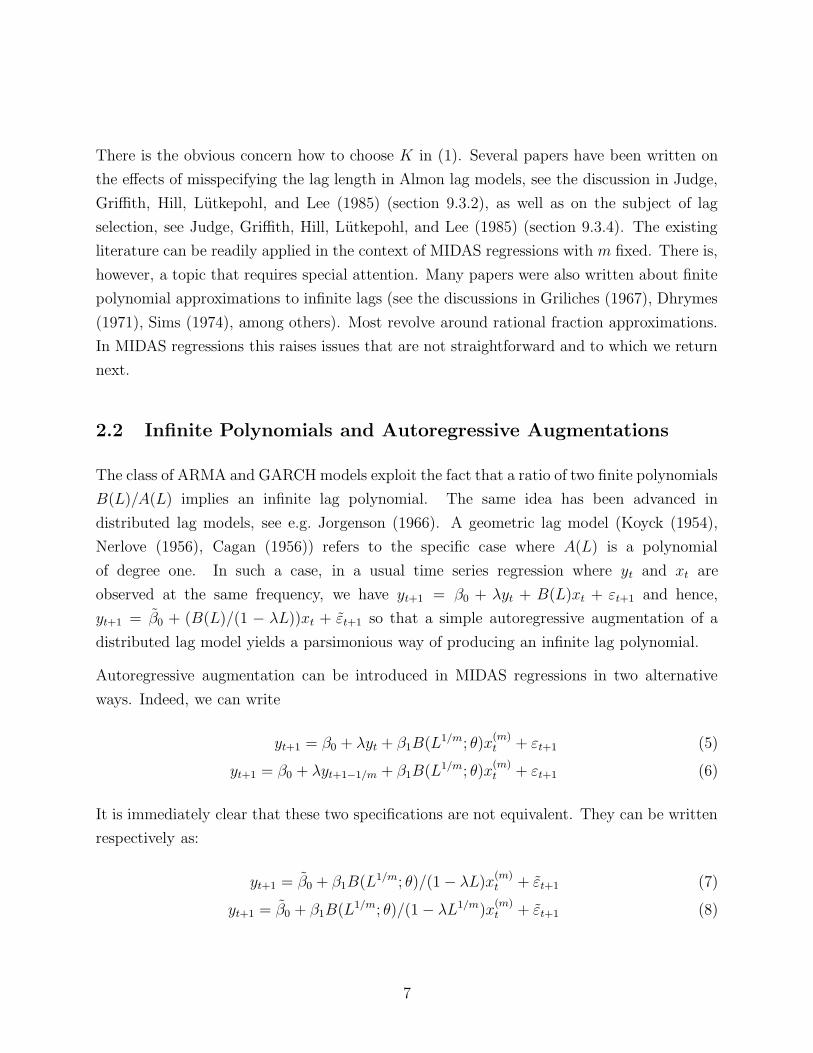
There is the obvious concern how to choose K in (1). Several papers have been written on
the effects of misspecifying the lag length in Almon lag models, see the discussion in Judge,
Griffith, Hill, Lutkepohl, and Lee (1985) (section 9.3.2), as well as on the subject of lag
selection, see Judge, Griffith, Hill, Lutkepohl, and Lee (1985) (section 9.3.4). The existing
literature can be readily applied in the context of MIDAS regressions with m fixed. There is,
however, a topic that requires special attention. Many papers were also written about finite
polynomial approximations to infinite lags (see the discussions in Griliches (1967), Dhrymes
(1971), Sims (1974), among others). Most revolve around rational fraction approximations.
In MIDAS regressions this raises issues that are not straightforward and to which we return
next.
2.2 Infinite Polynomials and Autoregressive Augmentations
The class of ARMA and GARCH models exploit the fact that a ratio of two finite polynomials
B(L)/A(L) implies an infinite lag polynomial. The same idea has been advanced in
distributed lag models, see e.g. Jorgenson (1966). A geometric lag model (Koyck (1954),
Nerlove (1956), Cagan (1956)) refers to the specific case where A(L) is a polynomial
of degree one. In such a case, in a usual time series regression where yt and xt are
observed at the same frequency, we have yt+1 = β0 + λyt + B(L)xt + εt+1 and hence,
yt+1 = β0 + (B(L)/(1 − λL))xt + εt+1 so that a simple autoregressive augmentation of a
distributed lag model yields a parsimonious way of producing an infinite lag polynomial.
Autoregressive augmentation can be introduced in MIDAS regressions in two alternative
ways. Indeed, we can write
yt+1 = β0 + λyt + β1B(L1/m; θ)x(m)t + εt+1 (5)
yt+1 = β0 + λyt+1−1/m + β1B(L1/m; θ)x(m)t + εt+1 (6)
It is immediately clear that these two specifications are not equivalent. They can be written
respectively as:
yt+1 = β0 + β1B(L1/m; θ)/(1 − λL)x(m)t + εt+1 (7)
yt+1 = β0 + β1B(L1/m; θ)/(1 − λL1/m)x(m)t + εt+1 (8)
7

Both specification should be used with the following caveats. In the case of (5), we do not
obtain a geometric polynomial in L1/m but rather a polynomial B(L1/m; θ)∑
j λjLj which is
a mixture with geometrically declining spikes at distance m. Hence, we obtain a “seasonal”
polynomial and this augmentation can be used only if there are seasonal patterns in x(m)t .
The second polynomial is geometric in L1/m and indeed yields B(L1/m; θ)∑
j λjLj/m.
However, it assumes that lagged yt+1−1/m are available. This amounts to considering a
special case of a distributed lag model. Moreover, specification (6) has some econometric
complications, since the appearance of y(m)t+1−1/m implies that one has to deal with endogenous
regressors and with instrumental variable estimation in a MIDAS context. Ghysels, Santa-
Clara, and Valkanov (2002) discuss the econometric implications, in particular efficiency
losses that occur due to the fact that the introduction of lagged dependent variables is most
often not possible in MIDAS regressions.
Despite these difficulties, the use of finite polynomial ratios to accommodate infinite lag
MIDAS specifications is still promising. For instance, consider the following MIDAS
regression:
yt = β0 + β1[B1K(L1/m)/B2Q(L1/m)]x(m) + εt ≡ β0 + β1
∑Kk=1 B1(k, θ)Lk/m
∑Qk=1 B2(k, θ)Lk/m
x(m)t + εt (9)
where K and Q are the respective orders of the polynomials in the numerator and
denominator. The specification in (9) is a MIDAS version of the rational distributed lag
model discussed in Jorgenson (1966). It should also be noted that Bollerslev and Wright
(2001) suggest to use smoothed periodogram estimators to deal with parameter proliferation
in the context of high-frequency financial data. Periodogram estimators are in essence infinite
parameters settings and typically imprecise in applications that do not involve very large
data sets.
2.3 Stepfunctions
The advantage of the MIDAS framework is that we maintain a relatively simple parametric
format and are also able to extend it easily to non-linear and multivariate settings as
discussed later. The drawback is that we have to use non-linear estimation methods since
all the polynomial lag structures are constrained via non-linear functional specifications. We
conclude the section with some observations about MIDAS with stepfunctions, introduced
8

in Forsberg and Ghysels (2004). These MIDAS regressions are inspired by the HAR model
of Corsi (2003) which was also used in Andersen, Bollerslev, and Diebold (2003). To define
a MIDAS regression with stepfunctions, consider regressors Xt(K, m) ≡∑K
j=1 x(m)t−j/m, which
are partial sums of high frequency x(m). Then the MIDAS regression with M steps is:
yt = β0 +M∑i=1
βiXt(Ki, m) + εt (10)
where K1 < . . . < KM . The impact of x(m)t is measured by
∑Mi=1 βi, since it appears in all
the partial sums (or steps). The impact of x(m)t−j for K1 < j K2 is measured by
∑Mi=2 βi.
Hence, the distributed lag patterns is approximated by a number of discrete steps. The
more steps appear in the regressions the less parsimonious, which defies the purpose of the
MIDAS regression approach. Yet, stepfunction approximations can be very useful and their
ease to estimate can be very appealing. Besides Forsberg and Ghysels (2004), MIDAS with
stepfunctions is also used in Ghysels, Sinko, and Valkanov (2004) to study the impact of
economic news on the cross-section of returns.
2.4 Identification issues
The stepfunctions discussed in the previous subsection have another advantage compared
to the generic MIDAS regression appearing in equation (1). Suppose we want to test the
hypothesis that βi = 0 ∀ i ≥ 1 in equation (10). In equation (1) the same hypothesis,
namely that none of the regressors are significant, comes with further complications since
the slope parameter β1 and the parameters in θ, governing the polynomial B(L1/m; θ), are
not separately identified under the null. Therefore testing such hypothesis involves testing
problems where nuisance parameters vanish under the null hypothesis and this in turn affects
the asymptotic distribution of the resulting test statistic.
There is a considerable literature on how to deal with hypothesis testing in the presence of
parameters that are not identified under the null. If θ were known, then the testing problem
could be formulated easily, namely β1 can be estimated via OLS, given θ, and hence yield an
estimate β1(θ). Testing the null hypothesis that β1 = 0 would not be complicated, namely
under conventional regularity conditions a heteroskedasticity-robust t-test takes the form:
WT (θ) = T β1(θ)′R(RV ∗
T R−1R′β1(θ)
9

where R is the selection matrix [01]′, and V ∗
T is a HAC covariance estimator of the parameters
associated with the OLS regression. Under standard regularity conditions this statistic has
point-optimal interpretation and χ21 limiting distribution as T → ∞. Davies (1977a) and
(1977b) suggested testing the null by supθ∈Θ WT (θ), where Θ is the parameter space assumed
to be a bounded subset of the reals. Hansen (1996) derive a distributional theory based on a
local-to-null reparameterization: β1 = c/√
T , with the null hypothesis now being c = 0 and
the alternative c 6= 0. To compute p-values, Hansen (1996) a simulation approach (see page
419). The solution of Davies (1977a) and (1977b) gives a straightforward, if conservative,
method for adjusting the testing statistic, whereas the Hansen (1996) simulation approach
should be less conservative.
3 Reverse Engineering the MIDAS Regression
One may still wonder whether it is necessary to use polynomials like the ones presented
in the previous section. In some cases, one can indeed formulate a time-series model for
the data sampled at frequency 1/m and compute the implied MIDAS regression which is
an exercise we shall call reverse engineering. The purpose of this section is to go through
such an exercise and to show that it is feasible only in some very special cases. However,
in general this approach appears to be an impractical alternative to MIDAS regressions.
The complexity of the reverse engineering will clarify the appeal of the route we advocate:
simplicity, flexibility, and parsimony.
We consider an example drawn from the volatility literature. To set the stage, let us
reconsider equation (1) where the right-hand side variable is y(m)t . In other words, yt is
observed at two frequencies. In addition, assume that both yt and y(m)t are generated by
a weak GARCH(1,1) process.4 More specifically, consider the so-called GARCH diffusion
which yields exact weak GARCH(1,1) discretization that are represented by the following
equations:
ln Pt − ln Pt−1/m = r(m)t = σ(m),tz
(m)t
σ2(m),t = φ(m) + α(m)[r
(m)t−1/m]2 + β(m)σ
2(m),t−1/m
(11)
4The terminology of weak GARCH originated with the work of Drost and Nijman (1993) and refersto volatility predictions involving only linear functionals of past returns and squared returns. Obviously,many ARCH-type models involve nonlinear functions of past (daily) returns. It would be possible to studynonlinear functions involving distributed lags of high frequency returns. This possibility is explored later inthe paper.
10

where z(m)t is Normal i.i.d. (0, 1) and r
(m)t is the returns process sampled at frequency 1/m.5
Suppose we run regression (1) between the (monthly) sum of squared returns and (daily)
squared returns, i.e., we estimate
m∑j=1
[r(m)t+j/m]2 = β0 + β1B(L1/m)[r
(m)t ]2 + εt (12)
then the resulting MIDAS regression would be:
β0 = (m + ρ(m))φ(m)
β1 = [mφ(m) + δ(m)]ρ(m)
B(L1/m) = [mφ(m) + δ(m)]∑
∞
k=0(β(m)/β1)kLk
(13)
where ρ(m) = 1/(1−β(m)) and δ(m) = (1− (α(m) +β(m))m)α(m)/(1−α(m)−β(m))(α(m) +β(m)).
Clearly, in this simple case, the MIDAS regression can be reverse engineered and would yield
estimates of the underlying weak GARCH(1,1) model or the GARCH diffusion.
The simplicity of this example may lead one to think that this path is promising. However,
as the following example shows, things become quite complicated when more realistic models
are used. In particular, many recent papers on volatility suggest that the process should be
modelled as a two-factor model. Ding and Granger (1996) and Engle and Lee (1999) suggest
a two-factor GARCH model. Two-factor stochastic volatility models have been proposed
by Alizadeh, Brandt, and Diebold (2002), Chacko and Viceira (1999), Gallant, Hsu, and
Tauchen (1999) and Chernov, Gallant, Ghysels, and Tauchen (2002). The latter study
provides a comprehensive comparison of various one- and two-factor continuous time models
and finds the log-linear two-factor model to be the most promising. Maheu (2002) shows
that the two-factor GARCH models can also take into account the long-range dependence
found in financial market volatility. In light of this, let us consider a two-factor GARCH
model where each factor follows a GARCH(1,1) process as specified in equations (1) through
(4) appearing in Appendix 6). This model yields a restricted GARCH(2,2) representation
5The GARCH parameters of (11) are related to the GARCH diffusion via formulas appearing inCorollary 3.2 of Drost and Werker (1996). Likewise, Drost and Nijman (1993) derive the mappings between
GARCH parameters corresponding to processes with r(m)t sampled with different values of m.
11

for (the observable process) h(m)t , namely:
h(m)t = (1 − ρ2(m))ω(m) + (α1(m) + α2(m))[ε
(m)t−1/m]2
−(ρ1(m)α2(m) + ρ2(m)α1(m))[ε(m)t−2/m]2
+(ρ1(m) + ρ2(m) − α1(m) − α2(m))h(m)t−1/m
−(ρ1(m)ρ2(m) − ρ1(m)α2(m) − ρ2(m)α1(m))h(m)t−2/m
where ρi(m), ω(m), αi(m) determine the volatility components, for i = 1,2, and are explicitly
defined in Appendix 6.
Using the computations in equations (5) through (8), which appears in Appendix 6, we can
derive the implied MIDAS regression, for a case where m = 4, applicable to a monthly/weekly
MIDAS regression setting. The intercept of the MIDAS regression is:
β0 = (1 − ρ2(m))ω(m)(4 − (ρ1(m) + ρ2(m)) − ρ1(m)ρ2(m) − (ρ1(m) + ρ2(m))2
−ρ1(m)ρ2(m) − (ρ1(m) + ρ2(m))ρ1(m)ρ2(m) − (ρ1(m) + ρ2(m))3 − 2(ρ1(m) + ρ2(m))×
ρ1(m)ρ2(m) − (ρ1(m) + ρ2(m))2ρ1(m)ρ2(m) − (ρ1(m)ρ2(m))
2 − (ρ1(m) + ρ2(m))4
−3(ρ1(m) + ρ2(m))2ρ1(m)ρ2(m) − (ρ1(m)ρ2(m))
2 − (ρ1(m) + ρ2(m))3ρ1(m)ρ2(m)
−2(ρ1(m) + ρ2(m))(ρ1(m)ρ2(m))2)
(14)
Despite the simplicity of the model and the low value of m we find that the implied MIDAS
polynomial is extremely complex and impractical. It appears in the Appendix as formula (9).
It is also worth noting that for stochastic volatility models the problem is even more difficult
since the volatility factors are latent and therefore need to be extracted from observed past
returns. This is an extremely difficult task to perform for which there are no analytical
closed-form solutions.6
The two examples in this section show that reverse engineering is not a practical solution,
except in some very limited circumstances. It should also be noted that this analysis is
confined to MIDAS regressions involving a pure autoregressive time-series setting without
additional regressors. If additional regressors are introduced, then reverse engineering
becomes simply impractical.
6See for instance Chernov, Gallant, Ghysels, and Tauchen (2002) for further discussion. Meddahi (2002)derives a weak GARCH(2,2) representation of a two-factor SV model which could be used in this particularcase, but not in a more general setting.
12

4 Variations on the MIDAS Regression Theme
In this section we cover a number of issues that come to the forefront when volatility dynamics
and its stylized facts are considered. In a first subsection we discuss some alternative
choices of volatility measures in the context of MIDAS regressions. The subject of nonlinear
equations and multivariate MIDAS regression models is vast and the purpose of the second
subsection is not to be comprehensive. The same observation applies to the final subsection
dealing with tick-by-tick applications.
4.1 More General Univariate MIDAS Linear Regression Models
A general univariate MIDAS linear regression model can be written as
yt+k = β0 +K∑
i=1
L∑j=1
Bij(L1/mi)x
(mi)t + εt+1 (15)
where Bij(L1/mi) are polynomials parameterized by the vector θ which we suppress for
simplicity. We will also suppress the double index to Bij when its presence is redundant. For
the purpose of exposition we will most often consider yt+k with k = 1. Equation (15) is a
conventional distributed lag model when K = 1, L = 1 and m1 = 1 and a single polynomial
MIDAS model when K = 1, L = 1 and m1 > 1. Moreover, the MIDAS regression involves
a single time series process when x(m1)t = y
(m1)t . We run a MIDAS regression where at least
two different sampling frequencies are combined when K > 1 and L = 1. A commonly
encountered case would be m1 = 1 and either one or more mi < 1. Such a MIDAS regression
would combine for instance monthly (daily) with daily (intra-daily) data to predict future
monthly (daily) series.
MIDAS regressions with L > 1 deserve some attention and to facilitate the discussion let us
assume that K = 1 with m1 > 1. This case corresponds to having two or more polynomials
with parameters θi = (θi1, θ
i2), i = 1, . . . , L that involve the same operator L1/m1 . To further
simplify the discussion, suppose that L = 2 and that θ11 = 1, θ1
2 > 1, θ21 > 1 and θ2
2 > θ21. We
plot one such example in Figure 3 using a mixture of two Beta lag polynomials. The first
polynomial, plotted in the top panel, is declining, whereas the second one, plotted in the
middle panel, is “hump shaped.” Mixing the two polynomials produces a third polynomial,
plotted in the bottom panel. From this example, it becomes clear that mixing polynomials
13

with the same high frequency lag operator would allow us to capture seasonal patterns or
rich non-monotone decay structures. However, the price for this flexibility will be a less
parsimonious specification as L increases.
4.2 Non-Linear MIDAS Regression Models
So far we carried out the analysis with the basic univariate MIDAS regression model. We
can further generalize the regression appearing in (15) to:
yt+k = β0 + f(K∑
i=1
L∑j=1
Bij(L1/mi)g(x
(mi)t )) + εt+1 (16)
where the functions f and g can either be known functions or else parameter dependent.
For example, in many volatility applications one takes the log transformation, i.e. one tries
to predict future log volatility (yt+k) and therefore takes f equal to log, with g(x) = x. One
parametric choice for g of interest in the context of volatility is the following:
yt+k = β0 +
K∑i=1
L∑j=1
Bij(L1/mi)(r
(m)t + θL|r(m)
t |)2 + εt+1 (17)
The above specification is very much inspired by the EGARCH model of Nelson (1991). We
reserve a particular parameter θL to test for leverage effects, when zero we obtain the linear
MIDAS regression model. A non-zero θL entails a response for positive returns that differs
from that of negative returns. The parameter θL is estimated jointly with the polynomial
parameters θ and any other parameters appearing in the MIDAS regression model.
Equation (17) could be viewed as a nonlinear MIDAS regression model that allows us to
investigate a particular issue, namely leverage. There are other models of this kind that
can be tailored to a specific question and we leave this topic for further research. It should
parenthetically be noted that the specification in (17) also applies to the risk-return trade-
off equation and possibly other settings as well. Ghysels, Santa-Clara, and Valkanov (2005)
indeed find that θL is significant with monthly/daily MIDAS regression regressions.
Another choice of a parameter dependent function g in (16) is the Box-Cox transformation,
which in the context of ARCH type models has been considered by Higgins and Bera
(1992), Ding, Granger, and Engle (1993), Hentschel (1995), and Duan (1997). In general,
14

non-linearities in MIDAS regressions can be handled without complications using standard
econometric approaches.
4.3 Tick-by-Tick Applications
Unequally spaced data is a topic of interest in finance and other areas (see e.g. Aıt-Sahalia
and Mykland (2003), Duffie and Glynn (2001), Dufour and Engle (2000), Engle (2000),
Ghysels and Jasiak (1998), Renault and Werker (2002) for some recent examples and further
references). The idea of a MIDAS regression where polynomial weights are governed by
hyperparameters is not necessarily limited to equal divisions of the reference interval. Hence,
instead of using the lag operator L1/m one can use an operator Lτ where τ is real-valued
instead of a rational number. When the MIDAS polynomial is for example of the Almon-type
then the weight for the τ th lag becomes:
b(k; θ) =eθ1k+...+θQkQ
∑Kk=1 eθ1k+...+θQkQ
where typically k is measured in time elapsed like a lag operator. Consequently, if we have
a data set of transactions data and are interested in predicting tomorrow’s volatility (t + 1)
using all the transactions data of the previous day or part of the previous day we can use,
say, [r(t,τi)]2, where the index (t, τi) refers to the time between to the close on day t and
transaction i on day t.
The unequally spaced applications have the virtue that one does not estimate the MIDAS
polynomial on a fixed, equally-spaced grid, but rather using past random events. Obviously,
it is not clear that microstructure noise may prevent us from putting this idea to work in
the context of volatility applications. There are, however, other areas of interest pertaining
to the microstructure of the market, such as measuring the price impact of trades, where
following a MIDAS approach applied to unequally spaced data may be useful.
15

4.4 Multivariate MIDAS Regression Models
We turn now to multivariate specifications. If we consider a linear MIDAS, we can further
generalize the regression appearing in (15) to:
Yt+1 = B0 +
K∑i=1
L∑j=1
Bij(L1/mi)X
(mi)t + εt+1 (18)
where Y, ε, and X are n-dimensional vector processes, B0 a n-dimensional vector and Bij
are n × n matrices of polynomials. The main issue of course is how to handle parameter
proliferation in multivariate settings. One approach would be to take all the off-diagonal
elements as controlled by one polynomial whereas the diagonal elements have a common
second polynomial. Such restrictions may not always be appropriate. Ultimately, the
restrictions that are needed to reduce the number of parameters will be dictated by the
application at hand.
Multivariate applications in the context of volatility would typically involve trading volume.
In principle, one can consider a MIDAS regression model explaining jointly future trading
volume and future volatility by past intra-daily trading volume and squared returns. This
application is very much in the spirit of univariate MIDAS regression volatility models.
Considering multivariate MIDAS regressions (18) allows us to address Granger causality
issues. It is of particular interest, because the notion of Granger causality, as put forth
in Granger (1969), is subject to temporal aggregation error that can disguise causality or
actually create spurious causality when a relevant process is omitted.7
While the MIDAS regression framework does not necessarily resolve all aggregation issues,
it might provide a convenient and powerful way of testing for Granger causality. Indeed, in
typical VAR models based on same-frequency regressions, Granger causality may be difficult
to detect due to temporal aggregation on the right-hand side variables. The restrictions on
the polynomials to test for causality are very much the same as those in the regular Granger
causality tests. It is also worth noting that MIDAS regression polynomials, univariate or
multivariate, can be two-sided, i.e., they can involve future realizations of x(m). This allows
us to conduct Granger causality tests as suggested by Sims (1972).
The multivariate specifications include systems of equations that can address ARCH-in-mean
7There is a considerable literature on the subject. See, e.g. Breitung and Swanson (2000) for a recentdiscussion.
16

effects. In particular, consider the system
rt+1 = b10 + b1B1(L1/m)[r
(m)t ]2 + ε1,t+1 (19)
Qt,t+1 = b20 + b2B2(L1/m)[r
(m)t ]2 + ε2,t+1
where the first equation in (19) refers to the return-volatility tradeoff and the second is
a volatility predictor, i.e. Qt,t+1 is next period’s realized volatility. If we restrict the
polynomials in the two equations to be equal and estimate the system simultaneously then
we have a model like the ARCH-in-mean specification. However, the flexibility of MIDAS
regression models also allows us to estimate the first and second equation in (19) separately,
and hence one can test the imposed polynomial restriction.
We can conclude this section with the observation that the MIDAS regressions are very
flexible. While we have attempted to be comprehensive in the variations of MIDAS
specifications, there are certainly interesting models that we have omitted. As with same-
frequency regressions, the specification of the model, be it multivariate or non-linear, will be
guided by the researchers’ agenda and ingenuity.
5 Two Empirical Examples
In this section we report on two empirical applications involving MIDAS regression models.
We revisit (1) the risk-return trade-off and (2) volatility prediction. Regarding the risk-
return trade-off, we present a variation of the results in Ghysels, Santa-Clara, and Valkanov
(2005) and Ghysels, Santa-Clara, and Valkanov (2003). Regarding volatility, we study the
impact of microstructure noise on volatility prediction. A subsection is devoted to each topic.
5.1 Revisiting the Risk-Return Tradeoff
In this subsection we revisit Merton’s (1973) ICAPM model, which suggests that the
conditional expected excess returns on the stock market should vary positively with the
market’s conditional variance:
Et[Rt+1] = µ + γV art[Rt+1], (20)
17

where γ is the coefficient of relative risk aversion of the representative agent. This relation
has received a lot of attention in empirical finance. The main difficulty in testing the ICAPM
resides in the fact that the conditional mean and variance of the market are not observable
and must be filtered from past returns. To quickly review the literature, Baillie and
DeGennaro (1990), French, Schwert, and Stambaugh (1987), Chou (1992), and Campbell and
Hentschel (1992) find a positive but insignificant relation between the conditional variance
and the conditional expected return. Using different methods, Campbell (1987) and Nelson
(1991) find a significantly negative relation, whereas Glosten, Jagannathan, and Runkle
(1993), Harvey (2001), and Turner, Startz, and Nelson (1989) find both a positive and a
negative relation depending on the method used. Other related papers are Chan, Karolyi,
and Stulz (1992), Lettau and Ludvigson (2002), Merton (1980), and Pindyck (1984).
In a recent paper, Ghysels, Santa-Clara, and Valkanov (2005) estimate equation (20) using
monthly returns as proxies for expected returns and daily squared returns in the estimation
of the conditional variance. In the specification of the MIDAS weights, they use the
Exponential Almon Lag (2) of second degree. Using CRSP value weighted returns from
January 1928 to December 2000, they find a positive and statistically significant risk-return
tradeoff. The authors argue that their significant and positive results obtain because their
MIDAS specification allows them to use monthly returns in specification of the mean and
daily squared returns in the estimation of the variance.
In another MIDAS paper, Ghysels, Santa-Clara, and Valkanov (2003) find that volatility can
be forecasted using daily regressors other than squared returns. They use MIDAS regressions
to predict realized volatility at weekly, two-weeks, three-weeks, and monthly horizons. The
authors show that better in- and out-of-sample estimates of the volatility are obtained when
the predictors on the right-hand side are daily absolute returns, daily realized volatilities,
daily ranges, and daily realized powers. The exact definitions of these predictors are provided
below. The daily realized volatility, daily ranges, and daily realized powers are obtained from
intra-daily (5 − minute) data of the Dow Jones index returns over the period from April
1993 to October 2003. Ghysels, Santa-Clara, and Valkanov (2003) show that the best overall
predictor of conditional volatility is the realized power and that, not surprisingly, better
forecasts are obtained at shorter (weekly) horizons.
In this subsection, we address several outstanding questions that arise from the previously
cited papers. First, is it possible to uncover a positive risk-return relation at frequencies from
one week to one month, given that volatility is well forecasted at high frequencies, but also
18

that our measure of expected returns grows increasingly noisier as the horizon decreases?
Second, can we improve on the estimation of the tradeoff by using predictors other than
squared daily returns? Third, would the results change if the parameters are specified as a
Beta Lag (3) function instead of an Exponential Almon Lag? Finally, there is also a question
of whether the Ghysels, Santa-Clara, and Valkanov (2005) results can be replicated using a
different dataset and a shorter sample period.
5.1.1 Methodology using MIDAS Regressions
We answer these questions by revisiting the risk-return equation (20) using the Dow Jones
index returns from April 1993 to October 2003. To estimate risk-return tradeoff parameter
γ using data at frequencies higher than a month, we obtain weekly, two-weeks, three-weeks,
and monthly returns from the 5 − minute price series. We denote the Dow Jones index
return over a horizon H as rt+H,t, similarly, we denote by rt day t return and rit the ith
5 − minute intra-daily return. We study horizons H of 5, 10, 15, and 22 days, respectively.
It is important to point out that returns are observed only once during a unit of time as
indicated by their subscript.
We consider the following regressions:
rt+H,t = µGH + γG
K∑k=0
B(k; θGm)r2
t−k + εGmt (21)
Expression (21) is a projection of rt+H,t onto lagged daily squared returns which corresponds
to the ARCH/GARCH-in-mean class of models (under some parameter restrictions). The
second equation determines the conditional volatility prediction, defining the MIDAS
polynomial∑K
k=0 B(k; θGm)r2
t−k as the prediction of volatility. Next we study two similar
models:
rt+H,t = µaH + γa
K∑k=0
B(k; θam)|rt−k| + εa
mt (22)
rt+H,t = µrH + γr
K∑k=0
B(k; θrm)[hi − lo]t−k + εr
mt (23)
Equations (22) and (23) involve projecting rt+H,t onto past daily absolute returns and daily
19

ranges, respectively, which are two alternative measures of volatility. Therefore they are
natural candidate regressors in the MIDAS specification (see e.g. Davidian and Carroll
(1987), Ding, Granger, and Engle (1993), Alizadeh, Brandt, and Diebold (2002) and Gallant,
Hsu, and Tauchen (1999)).
In the next equation (24), past RVt are used to predict rt+H,t as well as future realized
volatility. Examples of such models of volatility have been advocated by Andersen,
Bollerslev, and Diebold (2003) (and references cited therein).
rt+H,t = µQH + γQ
K∑k=0
B(k; θQm)RVt−k + εQ
mt (24)
The last regression (25) involves “realized power” defined as∑m
j=1 r2j,t, which has been
suggested by Barndorff-Nielsen and Shephard (2003) and Barndorff-Nielsen, Graversen, and
Shephard (2004). More specifically, Barndorff-Nielsen and Shephard suggest to consider the
sum of high-frequency absolute returns, or the realized power variation Pt, which is defined
as∑m
j=1 |rj,t|. Regression (25) projects future returns on past daily realized power.
rt+H,t = µpH + γp
K∑k=0
B(k; θPm)P
(m)t−k,t−k−1 + εp
mt (25)
We will estimate all five specifications under the alternative assumptions that the lag
coefficients B(k; θ) follow the Beta (3) or the Exponential Almon (2) parameterization.8
The latter specification has been used by Ghysels, Santa-Clara, and Valkanov (2005).
By comparing the Beta and Exponential Almon results, we investigate whether the
parameterizations are flexible enough to capture the dynamics of the underlying processes. If
the estimated coefficients of risk aversion γ are similar across the two specifications, then this
a strong indication that they are both successful at capturing the shape of the polynomial
weights.
It is also important to point out that, while the parametric form of the lag coefficients might
be the same across regressions, their shape will not be the same from predictor to predictor
and across horizons because the parameters θ will be different. As discussed at length above,
the flexible parametric specification of the lag weights is one of the defining characteristics
8Due to space limitations we will only report the Exponential Almon lag parameterization, the Beta oneis available on the web at http://www.unc.edu/~eghysels/papers/MIDAS_ER4.pdf.
20

of MIDAS regressions. For the estimates of γ to be directly comparable, all measures of
volatility are re-scaled to be in the same units for all horizons and across predictors.
Equations (21) - (25) are estimated at various frequencies using NLS. To correct for
heteroscedasticity we are using Newey-West corrected standard errors. The correction
window is chosen using the covariance matrix of the parameter estimates as A−1T BT A−1
T /T ,
where A−1T is an estimate of the Hessian matrix of the likelihood function and BT is an
estimate of the outer product of the gradient vector with itself applying the Bartlett kernel
window m = floor((4T/100)2/9).
5.1.2 Empirical results
The empirical results for equations (21) - (25) at one-, two-, three-, and four-week frequencies
appear in Table 1 (for Exponential Almon Lag weights (3)). The first two columns of the
table reports the intercept coefficient in expression (20) as well as the main parameter of
interest, γ. Newey-West t-statistics of γ under the null of no risk-return tradeoff are
shown in the third column. We report the mean absolute deviation (MAD) as a measure
of goodness of fit (fourth column), because it provides more robust results in the presence
of heteroskedasticity. The R2s are reported in the fifth column. The estimates of θ are not
reported since they do not have an economic interpretation. However, they determine the
shape of the polynomial lags B(k; θ) which are of clear economic interest. Hence, given the
estimates of θ, we report what fraction of the polynomial lags is placed on the first five
daily lag (column six), daily lags 6 to 20 (column seven), and lags beyond the first twenty
days (column eight). The weights are immediately available as fractions, because they have
previously been normalized to sum up to one.
The results in the table provide interesting answers to the questions that we raise in the
previous sub-section. First, at monthly frequency, there is a positive and statistically
significant risk-return tradeoff in the Dow Jones data for squared returns and absolute
returns only. The estimates of γ for the Exponential Almon and Beta polynomials (that
latter not reported in Table 1) are between 2.504 and 3.444 which is well within the bounds
of economically reasonable levels of risk aversion (see Hall (1988) and references therein).
This result also confirms the findings of Ghysels, Santa-Clara, and Valkanov (2005) who
find a γ estimate of 2.6 using a different dataset, shorter sample, and Exponential Almon
MIDAS weights. In addition, the γ estimated by the Exponential Polynomial is statistically
21

more significant than the Beta Polynomial gamma. Surprisingly, the estimates of monthly γ
computed using other measures of volatility are not significant but positive and within the
reasonable levels of risk aversion. This finding contradicts the evidence from Ghysels, Santa-
Clara, and Valkanov (2003) according to which the power variation and the realized volatility
predict future volatility better than the daily squared and absolute returns. For the Beta
Polynomial (not reported) the relation between conditional mean and conditional variance
is positive and statistically significant for most of the volatility measures for one-, two-, and
three-week horizons except for the realized volatility measure for three-week horizon and for
the range measure for two-week horizon. The findings are better than for the Almon lag
polynomial as far as statistical significance is concerned. It appears therefore that we recover
the results of Ghysels, Santa-Clara, and Valkanov (2005) with Dow-Jones data, yet ironically,
they are only obtained with the Beta Polynomial, whereas the Almon lag polynomial only
seems to work for the original setting of squared returns. In a sense, this is not so surprising
since Ghysels, Santa-Clara, and Valkanov (2003) advocate the use of the Beta Polynomial
when predicting volatility with high-frequency based volatility measures. It shows that there
are sometimes differences in the use of polynomials. We find that the power variation predicts
worse the risk-return trade-off than other volatility measures. This also finding contradicts
the results in Ghysels, Santa-Clara, and Valkanov (2003) showing that daily realized power
is a significantly better in- and out-of-sample predictor of future volatility. They also find
that daily range and daily quadratic variation significantly outperform squared daily returns
as predictors of future variance. There are at least two interpretations for this result. It
may appear that for the risk-return tradeoff the superiority of volatility forecasts seems not
to matter that much for this sample. Or, it may also be true that these variables forecast
a component of the variance that does not command compensation in terms of expected
returns. The results in the tables are not a direct test of any particular hypotheses, but they
are sufficiently robust across predictors and across horizons to lead us to believe that this
finding merits more careful analysis.
Overall, the direct comparison between the results Exponential Almon Beta polynomials
conveys a mixed message. On the one hand, the MAD goodness of fit measure demonstrates
that there is no difference between volatility measures and polynomial specifications. On
the other hand, comparison between short-time horizons γ coefficients demonstrates better
performance of the Beta polynomial specification. We interpret this results as an indication
that the Beta polynomial could be a better choice for the higher frequency models, whereas
the Exponential lag polynomial could be a better choice for the lower frequency. Overall the
22

differences are not so spectacular and one may wonder whether there are benefits using only
the relatively short samples of data for which intradaily data are available, as opposed to
the long span of daily data in the Ghysels, Santa-Clara, and Valkanov (2005) paper.
Next, we turn to Figures 4 and 5. The top two panels show respectively the Beta and
Exponential polynomials for the one week horizon and four week horizon. The top two
plots show the weights obtained with the empirical estimates of equations (21)- (25). In
Figure 4 we note that for realized power and absolute daily returns, the Beta and Almon
polynomials differ slightly across the various other regressors. At the four week horizon we
observe a hump-shaped pattern for realized power and also to a certain degree for daily
squared returns. It is also worth noting that the most regressors, and in particular realized
power, involve polynomials putting hardly any weight on longer lags. The four week horizon
quadratic variation polynomial is also quite different for the Beta and Almon polynomials.
The daily squared return decay pattern is similar to the one reported in Ghysels, Santa-
Clara, and Valkanov (2005), although the latter used a different estimator. Unlike the one
week horizon polynomials, we now observe more weight is put on the longer lags.
Finally, as expected, we also observe int Table 1) that the MAD increases steadily with the
horizon for all predictors. We also computed the MAD for a constant return prediction, see
Table 2. It is widely know that returns are hard to predict, and indeed with the regression
MAD results are compared with those unconditional return prediction MAD we do not see
much of an improvement. This is another way of saying that return predictions at such short
horizons usually lead to low R2s. Volatility predictions, in contrast yield much higher R2s
and this is the topic of the next subsection.
5.2 Volatility forecasting and microstructure noise
In this subsection we study forecasting future volatility using past volatility measures
unadjusted and adjusted for microstructure noise. The literature on the subject of market
microstructures and their impact on asset prices is considerable. The area covers many
aspects, ranging from: (1) price discreteness issues (see e.g., Harris (1990) (1990), Harris
(1991)); (2) asymmetries in information (see e.g., Glosten and Milgrom (1985), Easley and
O’Hara (1987), Easley and O’Hara (1992)); and (3) bid-ask spreads (see e.g., Roll (1984).)
Therefore, for a variety of reasons – including most prominently those mentioned above –
23

the efficiency price process is concealed by a veil of microstructure noise.9
The availability of high-frequency data in recent years led to extensive empirical research on
methods for studying the stylized facts and possibly correcting asset returns for the presences
microstructure noise. Since our focus is on predicting future volatility using the type of
regressions discussed in the previous subsection, we focus on corrections for microstructure
noise of RVt. There are many ways to approach the problem of adjusting increments in
quadratic variation for microstructure noise. A kernel-based correction was first introduced
by Zhou (1996) and further developed by Hansen and Lunde (2003), Barndorff-Nelsen,
Hansen, Lunde, and Shephard (2004) among others. Corrections based on sub-sampling
were introduced in Zhou (1996), Zhang, Mykland, and Aıt-Sahalia (2005b) and Zhang
(2005). Bandi and Russell (2005b) and Bandi and Russell (2005a) studied optimal sampling
in the presence of microstructure noise. Filtering, as an approach to microstructure noise
correction, was applied in Ebens (1999), Andersen, Bollerslev, Diebold, and Ebens (2001),
Maheu and McCurdy (2002) and Bollen and Inder (2002). Except for the work of Bollen and
Inder which uses the autoregressive filter, all other studies have used the moving average
filter. We will primarily use the corrections suggested in Hansen and Lunde (2003), who
present a comprehensive study of the recent developments.
5.2.1 Methods and data
To compare the performance of the different volatility measures, we use two adjusted
(RV 5min, RV 30min) and two unadjusted (RV 5minAC1
, RV 1tickACNW30
) volatility measures. The
subscripts 5min and 30min denote the sampling frequency of the returns used in the
construction of realized volatility. By definition, all returns used in these estimators are
equally spaced. Under the assumption that the microstructure noise is iid, RV 5minAC1
proposed
by Zhou (1996) provides a consistent estimator of the daily variance. Adopting the Hansen
and Lunde (2005) modification of the above estimator, we define (dropping the day t
subscript for notational convenience):
RV yAC1
= γy0 + 2γy
1 , γyj =
m
m − j
m−j∑i=1
ri,yri−1,y
where m is the number of 5-minutes returns per day (for DJIA stocks this number is 79).
9For additional references see O’Hara (1995), Hasbrouck (2004).
24

Instead of calendar-time (equally spaced time intervals), the RV 1tickACNW30
estimator uses
transactions-based data which is also referred to as tick-time. Hence, the 1tick estimator
makes use of all the available high-frequency data. The subscript ACNW, reflects the fact
that it estimator uses Newey-West kernel. Hansen and Lunde define the 1tick estimator as
follows
RV 1tickACNWk
= γ1tick0 + 2
k∑j=1
γ1tickj + 2
k∑j=1
k − j
kγ1tick
j+k , (26)
γ1tickj =
N
N − j
N−j∑i=1
ri,1tickri−1,1tick
where N is the number of observations available for the current day; N/(N − j) is a scaling
factor introduced to compensate for the ”missing” autocovariance terms.
To assess the forecasting performance, we follow the recent work of Ghysels, Santa-Clara,
and Valkanov (2003) who use MIDAS regressions to predict realized volatility at weekly,
two-weeks, three-weeks, and monthly horizons. In the context of forecasting the increments
in quadratic variation, denoted RV xy,(t+H,t) for horizon H with x and y taking the values
above - for example x = 5min and y = AC1 for the Zhou corrected RV estimates. For the
various measures we consider the following regressors:
RV xy,(t+H,t) = µQ
H + φQH
kmax∑k=0
bQH(k, θ)RV x
y,(t−k) + εQHt (27)
Hence, we compare how correcting for microstructure noise improves the forecasts of future
corrected increments and consider H equal to one week. Note that we consider uncorrected
measures of quadratic variation on both sides of equation (27). We use a Beta polynomial
which is particularly suitable for the application at hand.
The AA (Alcoa Inc) and MSFT (Microsoft) stocks are used as empirical examples. Figure
4 displays the daily volatility dynamics using the RV 5minAC1
volatility measures for the sample
considered by Hansen and Lunde (2005). The summary statistics for these two stocks are
in Table 3. The time series and summary statistics clearly demonstrate that the volatility
dynamics of the first part of the sample is quite different from the dynamics of the second
one. There is evidence of a structural change or regime switch, and this leads us to study
not only the entire sample but also two subsamples, respectively three and two years long.
25
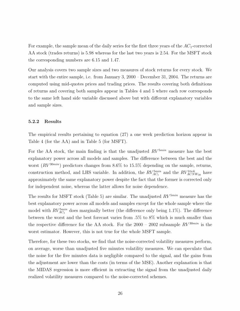
For example, the sample mean of the daily series for the first three years of the AC1-corrected
AA stock (trades returns) is 5.98 whereas for the last two years is 2.54. For the MSFT stock
the corresponding numbers are 6.15 and 1.47.
Our analysis covers two sample sizes and two measures of stock returns for every stock. We
start with the entire sample, i.e. from January 3, 2000 – December 31, 2004. The returns are
computed using mid-quotes prices and trading prices. The results covering both definitions
of returns and covering both samples appear in Tables 4 and 5 where each row corresponds
to the same left hand side variable discussed above but with different explanatory variables
and sample sizes.
5.2.2 Results
The empirical results pertaining to equation (27) a one week prediction horizon appear in
Table 4 (for the AA) and in Table 5 (for MSFT).
For the AA stock, the main finding is that the unadjusted RV 5min measure has the best
explanatory power across all models and samples. The difference between the best and the
worst (RV 30min) predictors changes from 8.6% to 15.5% depending on the sample, returns,
construction method, and LHS variable. In addition, the RV 5minAC1
and the RV 1tickACNW30
have
approximately the same explanatory power despite the fact that the former is corrected only
for independent noise, whereas the latter allows for noise dependence.
The results for MSFT stock (Table 5) are similar. The unadjusted RV 5min measure has the
best explanatory power across all models and samples except for the whole sample where the
model with RV 5minAC1
does marginally better (the difference only being 1.1%). The difference
between the worst and the best forecast varies from .5% to 8% which is much smaller than
the respective difference for the AA stock. For the 2000 – 2002 subsample RV 30min is the
worst estimator. However, this is not true for the whole MSFT sample.
Therefore, for these two stocks, we find that the noise-corrected volatility measures perform,
on average, worse than unadjusted five minutes volatility measures. We can speculate that
the noise for the five minutes data is negligible compared to the signal, and the gains from
the adjustment are lower than the costs (in terms of the MSE). Another explanation is that
the MIDAS regression is more efficient in extracting the signal from the unadjusted daily
realized volatility measures compared to the noise-corrected schemes.
26

To conclude, we turn again to Figures 4 and 5. The lower panel show respectively the RV 5min
and RV 1tickACNW30
regression polynomial estimates with the various past realized volatility
measures. We note that the estimated polynomial weights do not differ much across the
various regressors. This finding is in line with Ghysels, Santa-Clara, and Valkanov (2003).
The implication is that the differences in prediction performance comes entirely from the
choice of regressors, not the weighting schemes.
6 Conclusions
MIDAS regression models were recently introduced Ghysels, Santa-Clara, and Valkanov
(2002), (2003), (2005). This paper complements the current MIDAS literature by offerings
some new theoretical and empirical results. To explicitly demonstrate the need for mixed-
data sampling regressions, we show that the MIDAS results can be obtained with the
usual same-frequency time series regressions only in very specific cases. For more general
models, the MIDAS regressions clearly dominate. We also introduce several new MIDAS
specifications that include more general mixed-data structures, non-linearities, unequally
spaced observations, and multiple equations. Some of these specifications are straightforward
to estimate, other present particular challenges. One particularly attractive approach is
called MIDAS with stepfunctions. Although it sometimes defies the idea of parsimony, it
has the advantage of only involving linear regression models.
While we discuss a large variety of issues, there are clearly some areas that remain unresolved.
These areas pertain to multivariate and tick-by-tick applications, as well as long memory,
seasonality and other common time series themes like (fractional) co-integration.
27

Appendix: Reverse Engineering MIDAS Regressions –
A Two-Factor Model Example
We consider a two factor GARCH model, namely:
h(m)t = h
(m)1t + h
(m)2t (1)
with the components as follows:
h(m)1t = ω(m) + ρ1(m)h
(m)1t−1/m + α1(m)µ
(m)t−1/m (2)
and
h(m)2t = ρ2(m)h
(m)2t−1/m + α2(m)µ
(m)t−1/m (3)
where µ(m)t = [ε
(m)t ]2 − h
(m)t and returns are written as:
r(m)t = a(m) + ε
(m)t (4)
where a(m) is the conditional mean, ε(m)t = σ
(m)t z
(m)t and z
(m)t is i.i.d. (0, 1) while h
(m)t =
[σ(m)t ]2. The component GARCH model implies a restricted GARCH(2,2) representation for
(the observable process) h(m)t specified in 14. Using this representation we can compute the
following:
EL[h(m)t+1/m|Ih(m)
t ] = (1 − ρ2(m))ω(m)(1 − (ρ1(m) + ρ2(m)) − ρ1(m)ρ2(m)) + (ρ1(m) + ρ2(m))h(m)t
+ρ1(m)ρ2(m)h(m)t−1/m − (ρ1(m) + ρ2(m) − α1(m) − α2(m))µt
+(ρ1(m)ρ2(m) − ρ1(m)α2(m) − ρ2(m)α1(m))µt−1/m
(5)
EL[h(m)t+2/m|Ih(m)
t ] = (1 − ρ2(m))ω(m)(1 − (ρ1(m) + ρ2(m))2 − ρ1(m)ρ2(m) − (ρ1(m) + ρ2(m))×
ρ1(m)ρ2(m)) + ((ρ1(m) + ρ2(m))2 + ρ1(m)ρ2(m))h
(m)t + (ρ1(m) + ρ2(m))×
ρ1(m)ρ2(m)h(m)t−1/m − ((ρ1(m) + ρ2(m))(ρ1(m) + ρ2(m) − α1(m) − α2(m))
+(ρ1(m)ρ2(m) − ρ1(m)α2(m) − ρ2(m)α1(m)))µt
+ρ1(m)ρ2(m)(ρ1(m)ρ2(m) − ρ1(m)α2(m) − ρ2(m)α1(m))µt−1/m
(6)
28

EL[h(m)t+3/m|Ih(m)
t ] = (1 − ρ2(m))ω(m)(1 − (ρ1(m) + ρ2(m))3 − 2(ρ1(m) + ρ2(m))ρ1(m)ρ2(m)
−(ρ1(m) + ρ2(m))2ρ1(m)ρ2(m) − (ρ1(m)ρ2(m))
2) + ((ρ1(m) + ρ2(m))3
+2(ρ1(m) + ρ2(m))ρ1(m)ρ2(m))h(m)t + ((ρ1(m) + ρ2(m))
2ρ1(m)ρ2(m)
+(ρ1(m)ρ2(m))2)h
(m)t−1/m − ((ρ1(m) + ρ2(m))
2(ρ1(m) + ρ2(m) − α1(m) − α2(m))
−ρ1(m)ρ2(m)(ρ1(m) + ρ2(m) − α1(m) − α2(m))
+(ρ1(m) + ρ2(m))(ρ1(m)ρ2(m) − ρ1(m)α2(m)
−ρ2(m)α1(m)))µt + ((ρ1(m) + ρ2(m))2(ρ1(m)ρ2(m)
−ρ1(m)α2(m) − ρ2(m)α1(m)) + ρ1(m)ρ2(m)×(ρ1(m)ρ2(m) − ρ1(m)α2(m) − ρ2(m)α1(m)))µt−1/m
(7)
EL[h(m)t+4/m|Ih(m)
t ] = (1 − ρ2(m))ω(m)(1 − (ρ1(m) + ρ2(m))4 − 3(ρ1(m) + ρ2(m))
2ρ1(m)ρ2(m)
−(ρ1(m)ρ2(m))2 − (ρ1(m) + ρ2(m))
3ρ1(m)ρ2(m) − 2(ρ1(m) + ρ2(m))(ρ1(m)ρ2(m))2)
+((ρ1(m) + ρ2(m))4 + 3(ρ1(m) + ρ2(m))
2ρ1(m)ρ2(m) + (ρ1(m)ρ2(m))2)h
(m)t
+((ρ1(m) + ρ2(m))3ρ1(m)ρ2(m) + 2(ρ1(m) + ρ2(m))(ρ1(m)ρ2(m))
2)h(m)t−1/m
−((ρ1(m) + ρ2(m))3(ρ1(m) + ρ2(m) − α1(m) − α2(m))
+(ρ1(m) + ρ2(m))2(ρ1(m)ρ2(m) − ρ1(m)α2(m) − ρ2(m)α1(m))
−2(ρ1(m) + ρ2(m))ρ1(m)ρ2(m)(ρ1(m) + ρ2(m) − α1(m)
−α2(m)) + ρ1(m)ρ2(m)(ρ1(m)ρ2(m) − ρ1(m)α2(m) − ρ2(m)α1(m)))µt
+((ρ1(m) + ρ2(m))3 + 2(ρ1(m) + ρ2(m))ρ1(m)ρ2(m)(ρ1(m)ρ2(m)
−ρ1(m)α2(m) − ρ2(m)α1(m)))µt−1/m
(8)
Then the MIDAS projection equation has the following expression:
β1B(L1/m) = ((ρ1(m) + ρ2(m)) + (ρ1(m) + ρ2(m))2 + ρ1(m)ρ2(m) + (ρ1(m)+
ρ2(m))3 + 2(ρ1(m) + ρ2(m))ρ1(m)ρ2(m)
+(ρ1(m) + ρ2(m))4 + 3(ρ1(m) + ρ2(m))
2ρ1(m)ρ2(m) + (ρ1(m)ρ2(m))2)
+(ρ1(m)ρ2(m) + (ρ1(m) + ρ2(m))ρ1(m)ρ2(m) + (ρ1(m) + ρ2(m))2ρ1(m)ρ2(m)
+(ρ1(m)ρ2(m))2 + (ρ1(m) + ρ2(m))
3ρ1(m)ρ2(m)
+2(ρ1(m) + ρ2(m))(ρ1(m)ρ2(m))2)L1/m
+((ρ1(m)ρ2(m) − ρ1(m)α2(m) − ρ2(m)α1(m)) − (ρ1(m) + ρ2(m))×
29

(ρ1(m) + ρ2(m) − α1(m) − α2(m)) − (ρ1(m) + ρ2(m) − α1(m) − α2(m))
−(ρ1(m) + ρ2(m))2(ρ1(m) + ρ2(m) − α1(m) − α2(m))
−ρ1(m)ρ2(m)(ρ1(m) + ρ2(m) − α1(m) − α2(m))
+(ρ1(m) + ρ2(m))(ρ1(m)ρ2(m) − ρ1(m)α2(m) − ρ2(m)α1(m))
+(ρ1(m) − ρ2(m))3(ρ1(m) + ρ2(m) − α1(m) − α2(m)) + (ρ1(m)
+ρ2(m))2(ρ1(m)ρ2(m) − ρ1(m)α2(m) − ρ2(m)α1(m))
−2(ρ1(m) + ρ2(m))ρ1(m)ρ2(m)(ρ1(m) + ρ2(m) − α1(m) − α2(m))
+ρ1(m)ρ2(m)(ρ1(m)ρ2(m) − ρ1(m)α2(m) − ρ2(m)α1(m)))×(1 − (ρ1(m) + ρ2(m))L
1/m + ρ1(m)ρ2(m)L2/m)/
(1 − (ρ1(m) + ρ2(m) − α1(m) − α2(m))L1/m + (ρ1(m)ρ2(m) − ρ1(m)α2(m) − ρ2(m)α1(m))L
2/m)
+((ρ1(m)ρ2(m) − ρ1(m)α2(m) − ρ2(m)α1(m)) + ρ1(m)ρ2(m)×(ρ1(m)ρ2(m) − ρ1(m)α2(m) − ρ2(m)α1(m))+
(ρ1(m) + ρ2(m))2(ρ1(m)ρ2(m) − ρ1(m)α2(m) − ρ2(m)α1(m)) + ρ1(m)ρ2(m)(ρ1(m)ρ2(m)
−ρ1(m)α2(m) − ρ2(m)α1(m)) + (ρ1(m) + ρ2(m))3
+2(ρ1(m) + ρ2(m))ρ1(m)ρ2(m)(ρ1(m)ρ2(m) − ρ1(m)α2(m) − ρ2(m)α1(m)))×(1 − (ρ1(m) + ρ2(m))L
1/m + ρ1(m)ρ2(m)L2/m)L1/m/
(1 − (ρ1(m) + ρ2(m) − α1(m) − α2(m))L1/m + (ρ1(m)ρ2(m) − ρ1(m)α2(m) − ρ2(m)α1(m))L
2/m)
(9)
30

References
Aıt-Sahalia, Y., and P. Mykland, 2003, The effects of random and discrete samping when
estimating continuous time diffusions, Econometrica 71, 483–549.
Aıt-Sahalia, Yacine, Per Mykland, and Lan Zhang, 2005, How Often to Sample a Continuous-
Time Process in the Presence of Market Microstructure Noise, Review of Financial Studies
18, 351–416.
Alizadeh, Sassan, Michael W. Brandt, and Francis Diebold, 2002, Range-based estimation
of stochastic volatility models, Journal of Finance 57, 1047–1091.
Almon, S., 1965, The distributed lag between capital appropriations and expenditures,
Econometrica 33, 178–196.
Andersen, Torben G., Tim Bollerslev, and Francis X. Diebold, 2003, Some like it smooth,
and some like it rough: Untangeling continuous and jumps components in measuring,
modeling, and forecasting asset return volatility, Duke University, NC, USA.
, and Heiko Ebens, 2001, The distribution of realized stock return volatility, Journal
of Financial Economies 61, 43–76.
Angel, Leon, Juan Nave, and Gonzalo Rubio, 2004, The Relationship between Risk and
Expected Return in Europe, Discussion Paper.
Baillie, Richard T., and Ramon P. DeGennaro, 1990, Stock returns and volatility, Journal
of Financial and Quantitative Analysis 25, 203–214.
Bandi, Federico, and Jeffrey Russell, 2005a, Microstructure noise, realized variance, and
optimal sampling, Discussion Paper.
, 2005b, Separating microstructure noise from volatility, Journal of Financial
Economies forthcoming.
Barndorff-Nelsen, O. E., P. R. Hansen, A. Lunde, and N. Shephard, 2004, Regular and
modified kernel-based estimators of integrated variance: The case with independent noise,
http://www.stanford.edu/people/peter.hansen.
Barndorff-Nielsen, O., S. Graversen, and N. Shephard, 2004, Power variation and stochastic
volatility: a review and some new results, Journal of Applied Probability 41A, 133–143.
31

Barndorff-Nielsen, O., and N. Shephard, 2003, Power variation with stochastic volatility and
jumps, Bernoulli 9, 243–265.
Bollen, B., and B. Inder, 2002, Estimating daily volatility in financial markets utilizing
intraday data, Journal of Empirical Finance 9, 551–562.
Bollerslev, Tim, and Jeffrey M. Wooldridge, 1992, Quasi-maxmimum likelihood estimation
and inference in dynamic models with time-varying covariances, Econometric Reviews 11,
143–172.
Bollerslev, T., and J. H. Wright, 2001, Volatility forecasting, high-frequency data, and
frequency domain inference, Review of Economic Statistics 83, 596–602.
Breitung, J., and N. R. Swanson, 2000, Temporal aggregation and causality in multiple time
series models, Journal of Time Series Analysis 23, 651–665.
Brown, David, and Miguel Ferreira, 2004, Information in the Idiosyncratic Volatility of Small
Firms, Discussion Paper.
Cagan, P., 1956, The monetary dynamics of hyper inflations, in M. Friedman, ed.: Studies
in the Quantity Theory of Money. University of Chicago Press, Chicago.
Campbell, John Y., 1987, Stock returns and the term structure, Journal of Financial
Economies 18, 373–399.
, and Ludger Hentschel, 1992, No news is good news: An asymmetric model of
changing volatility in stock returns, Journal of Financial Economies 31, 281–318.
Chacko, George, and Luis Viceira, 1999, Spectral gmm estimation of continuous-time
processes, Working paper, Harvard Business School.
Chan, K. C., G. Andrew Karolyi, and Rene M. Stulz, 1992, Global financial markets and
the risk premium on U.S. equity, Journal of Financial Economies 32, 137–167.
Charoenrook, Anchada, and Jennifer Conrad, 2005, Identifying Risk-Based Factors,
Discussion Paper.
Chernov, Mikhael, A. Ronald Gallant, Eric Ghysels, and George Tauchen, 2002, Alternative
Models for Stock Price Dynamics, Journal of Econometrics 116, 225–257.
32

Chou, Ray, 1992, Volatility persistence and stock valuations: some empirical evidence using
GARCH, Journal of Applied Econometrics 3, 279–294.
Corsi, Fulvio, 2003, A simple long memory model of realized volatility, Unpublished
manuscript, University of Southern Switzerland.
Davidian, M., and R.J. Carroll, 1987, Variance function estimation, Journal of American
Statistical Association 82, 1079–1091.
Davies, R., 1977a, Hypothesis Testing when a Nuissance Parameter is Present Only under
the Alternative, Biometrika 64, 247–254.
, 1977b, Hypothesis Testing when a Nuissance Parameter is Present Only under the
Alternative, Biometrika 74, 33–34.
Dhrymes, P., 1971, Distributed lags: Problems of Estimation and Formulation (Holden-Day,
San Francisco).
Ding, Z., and C. Granger, 1996, Modeling volatility persistence of speculative returns: A
new approach, Journal of Econometrics 73, 185–215.
, and R.F. Engle, 1993, A long memory property of stock market returns and a new
models, Journal of Empirical Finance 1, 83–106.
Drost, F. C., and T. Nijman, 1993, Temporal aggregation of garch processes, Econometrica
61, 909–727.
Drost, F. C., and B.M.J. Werker, 1996, Closing the garch gap: Continuous time garch
modeling, Journal of Econometrics 74, 31–57.
Duan, J.-C., 1997, Augmented garch(p,q) process and its diffusion limit, Journal of
Econometrics 79, 97–127.
Duffie, D., and P. Glynn, 2001, Estimation of continuous-time markov processes sampled at
random time intervals, Discussion paper Stanford University.
Dufour, A., and R.F. Engle, 2000, Time and the price impact of a trade, Journal of Finance
55, 2467–2498.
Easley, D., and M. O’Hara, 1987, Price, trade size, and information in securities markets,
Journal of Financial Economies 16, 69–90.
33

, 1992, Time and the process of security price adjustment, Journal of Finance 47,
905–927.
Ebens, H., 1999, Realized stock volatility, Working paper 420, john Hopkins University.
Engle, R.F., 2000, The econometrics of high frequency data, Econometrica 68, 1–22.
, and G. Lee, 1999, A long-run and short-run component model of stock return
volatility, in Cointegration, Causality and Forecasting - A Festschrift in Honour of Clive
W. J. Granger. Oxford University Press.
Forsberg, Lars, and Eric Ghysels, 2004, Why do absolute returns predict volatility so well?,
UNC at Chapel Hill.
French, Kenneth R., William Schwert, and Robert F. Stambaugh, 1987, Expected stock
returns and volatility, Journal of Financial Economies 19, 3–29.
Gallant, A. Ronald, C.-T. Hsu, and George Tauchen, 1999, Using daily range data to
calibrate volatility diffusions and extract the forward integrated variance, Review of
Economic Statistics 81, 617–631.
Ghysels, E., and J. Jasiak, 1998, Garch for irregularly spaced financial data: The acd-garch
model, Studies in Nonlinear Dynamics and Econometrics 2, 133–149.
Ghysels, Eric, Pedro Santa-Clara, and Rossen Valkanov, 2002, The MIDAS touch: Mixed
data sampling regression models, Working paper, UNC and UCLA.
, 2003, Predicting volatility: getting the most out of return data sampled at different
frequencies, Journal of Econometrics forthcoming.
, 2005, There is a risk-return tradeoff after all, Journal of Financial Economics 76,
509–548.
Ghysels, Eric, Arthur Sinko, and Rossen Valkanov, 2004, The Cross Section of Firm Stock
Returns and Economic Announcements: A Bird’s Eye View, Working paper, UNC and
UCSD.
Glosten, L., and P. Milgrom, 1985, Bid, ask and transaction prices in a specialist market
with heterogeneously informed traders, Journal of Financial Economies 13, 71–100.
34

Glosten, Lawrence R., Ravi Jagannathan, and David E. Runkle, 1993, On the relation
between the expected value and the volatility of the nominal excess return on stocks,
Journal of Finance 48, 1779–1801.
Granger, C., 1969, Investigating causal relations by econometric models and cross spectral
methods, Econometrica 37, 428–438.
Griliches, Z., 1967, Distributed Lags: A Survey, Econometrica 35, 16–49.
Hall, Robert E., 1988, Intertemporal substitution in consumption, Journal of Political
Economy 96, 339–357.
Hansen, B., 1996, Inference when a Nuissance Parameter is not Identified Under the Null
Hypothesis, Econometrica 64, 413–430.
Hansen, Peter, and Asgar Lunde, 2004, An unbiased measure of realized variance,
forthcoming.
Hansen, P., and A. Lunde, 2005, Realized variance and market microstructure noise, Journal
of Business and Economic Statistics 9, 551–562.
Hansen, P. R., and A. Lunde, 2003, An optimal and unbiased measure of realized variance
based on intermittent high-frequency data, Discussion paper.
Harris, L., 1990, Estimation of stock variance and serial covariance from discrete
observations, Journal of Financial and Quantitative Analysis 25, 291–306.
, 1991, Stock price clastering and discreteness, Review of Financial Studies 25, 291–
306.
Harvey, Campbell R., 2001, The specification of conditional expectations, Journal of
Empirical Finance 8, 573–638.
Hasbrouck, J., 2004, Empirical Market Microstructure: Economic and Statistical
Perspectives on the Dynamics of Trade in Securities Markets. (Lecture Notes, Stern School
of Business, New York University.).
Hentschel, Ludger, 1995, All in the family: Nesting symmetric and asymmetric GARCH
models, Journal of Financial Economics 39, 71–104.
35

Higgins, M., and A. Bera, 1992, A class of nonlinear arch models, International Economic
Review 33, 137–158.
Jiang, Xiaoquan, and Bong-Soo Lee, 2004, On the Dynamic Relation between Returns and
Idiosyncratic Volatility, Discussion Paper.
Jorgenson, D.W., 1966, Rational Distributed Lag Functions, Econometrica 34, 135–149.
Judge, G., W.E. Griffith, R.C. Hill, H. Lutkepohl, and T.C. Lee, 1985, The theory and
Practice of Econometrics - Second Edition (John Wiley & Sons).
Koyck, L.M., 1954, Distributed Lags and Investment Analysis (North-Holland, Amsterdam).
Lettau, Martin, and Sydney C. Ludvigson, 2002, Measuring and modeling variation in the
risk-return tradeoff, in Yacine Ait-Sahalia, and Lars P. Hansen, ed.: Handbook of Financial
Econometrics.
Maheu, J., 2002, Can garch models capture the long-range dependence in financial market
volatility?, Unpublished manuscript, University of Toronto.
, and T. McCurdy, 2002, Nonlinear features of realized fx volatility, Review of
Economics and Statistics 84, 668–681.
Meddahi, N., 2002, Arma representation of two-factor models, Discussion paper, Universite
de Montreal.
Merton, Robert C., 1973, An intertemporal capital asset pricing model, Econometrica 41,
867–887.
, 1980, On estimating the expected return on the market: An exploratory
investigation, Journal of Financial Economies 8, 323–361.
Nelson, Daniel B., 1991, Conditional heteroskedasticity in asset returns: A new approach,
Econometrica 59, 347–370.
Nerlove, M., 1956, Estimates of the elasticities of supply of selected agricultural commodities,
Journal of Farm Economics 38, 496–509.
O’Hara, M., 1995, Market Microstructure Theory (Blackwell).
36

Pindyck, Robert S., 1984, Risk, inflation, and the stock market, American Economic Review
74, 335–351.
Renault, E., and B. Werker, 2002, Stochastic volatility models with transactions time risk,
Discussion paper, CIRANO, Montreal.
Roll, R., 1984, A simple implicit measure of the bid-ask spread in an efficient market, Journal
of Finance 39, 1127–1139.
Sims, C.A., 1972, Money, income, and causality, American Economic Review 62, 540–552.
, 1974, Distributed lags, in Michael D. Intrilligator, and David A. Kendrick, ed.:
Frontiers of Quantitative Economics II. North-Holland, Amsterdam.
Turner, Christopher M., Richard Startz, and Charles R. Nelson, 1989, A markov model of
heteroskedasticity, risk, and learning in the stock market, Journal of Financial Economies
25, 3–22.
Wang, Leping, 2004, On the Intertemporal Risk-Return Relation: A Bayesian Model
Comparison Perspective, Discussion Paper.
Zhang, L., 2005, Efficient estimation of stochastic volatility using noisy observations: A
multi-scale approach, Research Paper, Carnegie Mellon University.
Zhang, Lan, Per Mykland, and Yacine Aıt-Sahalia, 2005a, A Tale of Two Time Scales:
Determining Integrated Volatility with Noisy High-Frequency Data, Journal of American
Statistical Association forthcoming.
Zhang, L., P. A. Mykland, and Y. Aıt-Sahalia, 2005b, A tale of two time scales: Determining
integrated volatility with noisy high frequency data, Journal of the American Statistical
Association forthcoming.
Zhou, B., 1996, High-frequency data and volatility in foreign-exchange rates, Journal of
Business and Economic Statistics 14, 45–52.
37

Table 1: Results of the Risk-Return Tradeoff using MIDAS Models with Daily
Regressors - Dow Jones Returns with Exponential Almon Polynomial
The table shows results from estimating equations (21-25) at one-, two-, three-, and four-week frequencies.The MIDAS weights are parameterized to follow the Exponential Almon polynomial (2). The estimationis performed by quasi-maximum likelihood using Dow Jones index return data from April 1993 to October2003. The estimates of µ and γ are displayed in the first two columns. In column three, we show thet-statistic of γ under the null of no risk-return tradeoff and the standard errors are computed using theheteorskedasticity-robust Bollerslev and Wooldridge (1992) method. We compute in column four the meanabsolute deviation (MAD) as a measure of the goodness of fit of the MIDAS regression, because it is robustto heteroskedasticity in the data. The fraction of the weights placed on lags 1 to 5 (one week), lags 6 to 20(one month), and higher, are shown in columns five to seven, respectively. The panels contain the resultsfor squared daily returns (r2
t ), absolute daily returns (|rt|), daily ranges ([hi − lo]t), daily realized volatility(Qt), and daily realized power (Pt), as explained in the text.
Sample April 1993 - October 2003
µ γ t − stat MAD R2 days 1-5 days 6-20 > 20 days
Daily r2t
1 wks -0.001 4.533 0.848 0.018 0.013 0.658 0.328 0.0142 wks -0.000 2.528 3.350 0.023 0.026 0.990 0.010 0.0003 wks -0.001 2.950 0.529 0.029 0.039 1.000 0.000 0.0004 wks -0.001 2.490 3.915 0.032 0.034 0.998 0.002 0.000
Daily |rt|1 wks -0.004 9.618 2.868 0.018 0.020 1.000 0.000 0.0002 wks -0.006 7.600 2.962 0.023 0.029 1.000 0.000 0.0003 wks -0.008 7.630 2.387 0.030 0.034 0.002 0.998 0.0004 wks -0.004 3.444 2.670 0.033 0.029 1.000 0.000 0.000
Daily [hi − lo]t1 wks -0.004 10.878 2.264 0.018 0.014 1.000 0.000 0.0002 wks -0.006 8.144 1.432 0.024 0.020 0.130 0.870 0.0003 wks -0.009 8.395 2.016 0.030 0.028 0.016 0.984 0.0004 wks -0.005 4.630 1.666 0.033 0.018 1.000 0.000 0.000
Daily Qt
1 wks -0.001 5.036 2.558 0.018 0.013 1.000 0.000 0.0002 wks -0.003 5.006 2.397 0.024 0.024 0.336 0.664 0.0003 wks -0.003 4.116 1.460 0.029 0.026 0.335 0.665 0.0004 wks -0.001 2.524 1.012 0.033 0.014 0.618 0.374 0.007
Daily Pt
1 wks -0.004 9.523 0.000 0.018 0.009 1.000 0.000 0.0002 wks -0.005 6.899 1.480 0.024 0.011 0.275 0.725 0.0003 wks -0.006 6.022 1.244 0.030 0.015 0.177 0.823 0.0004 wks -0.004 4.104 1.137 0.033 0.010 0.990 0.010 0.000
38

Table 2: Summary statistics - Dow Jones Returns.
Sample April 1993 - October 2003
mean V ar MAD
1 wks 0.002 0.001 0.0182 wks 0.004 0.001 0.0243 wks 0.006 0.001 0.0304 wks 0.008 0.002 0.033
39

Table 3: Summary Statistics for the AA and MFST StocksEach entry in the table corresponds to the sample mean for the different daily volatility measure and different subsample. Subsample 2000- 2002 covers January 3, 2000 - December 31, 2002. Subsample 2003 - 2004 covers January 3, 2003 - December 31, 2004. The name of thevariables are consistent with the notation in Hansen and Lunde (2005) (2005) paper.
2000− 2002 2003− 2004
RV 5min RV 30min RV 5minAC1
RV 1tickACNW30
RV 5min RV 30min RV 5minAC1
RV 1tickACNW30
AA
Mid Quotes 5.627 5.676 5.883 5.979 2.557 2.561 2.565 2.755Trades 6.121 5.805 5.979 5.962 2.616 2.576 2.549 2.667
MSFT
Mid Quotes 6.005 5.537 6.168 6.125 1.712 1.471 1.472 1.788Trades 6.182 5.560 6.149 6.039 1.746 1.475 1.465 1.791
40

Table 4: R2 Comparison of MIDAS Models for One Week Horizon - AA StockEach entry in the table corresponds to the R2 for different models (24) and different estimation samples. The whole sample covers January3, 2000 - December 31, 2004. Subsample 2000 - 2002 covers January 3, 2000 - December 31, 2002. The regressions are run on a weekly (5days) data sampling scheme. The name of the variables are consistent with the notation in Hansen and Lunde (2005) (2005) paper. Everycolumn corresponds to the explanatory power of the different LHS variables for the same RHS variable.
2000− 2004 2000− 2002
Model RV 5min RV 30min RV 5minAC1
RV 1tickACNW30
RV 5min RV 30min RV 5minAC1
RV 1tickACNW30
Mid quotesRV 5min 0.651 0.536 0.599 0.593 0.514 0.360 0.471 0.483RV 30min 0.503 0.417 0.482 0.464 0.406 0.298 0.388 0.393RV 5min
AC10.597 0.503 0.568 0.548 0.444 0.335 0.421 0.434
RV 1tickACNW30
0.586 0.484 0.547 0.531 0.464 0.330 0.437 0.442Trades
RV 5min 0.666 0.566 0.624 0.603 0.525 0.396 0.497 0.483RV 30min 0.510 0.422 0.485 0.467 0.413 0.303 0.395 0.394RV 5min
AC10.601 0.513 0.573 0.553 0.450 0.351 0.435 0.438
RV 1tickACNW30
0.558 0.465 0.532 0.505 0.428 0.307 0.411 0.397
41

Table 5: R2 Comparison of MIDAS Models for One Week Horizon - MSFT StockEach entry in the table corresponds to the R2 for different models (24) and different estimation samples. The whole sample covers January3, 2000 - December 31, 2004. Subsample 2000 - 2002 covers January 3, 2000 - December 31, 2002. The regressions are run on a weekly (5days) data sampling scheme. The name of the variables are consistent with the notation in Hansen and Lunde (2005) (2005) paper. Everycolumn corresponds to the explanatory power of the different LHS variables for the same RHS variable.
2000− 2004 2000− 2002
Model RV 5min RV 30min RV 5minAC1
RV 1tickACNW30
RV 5min RV 30min RV 5minAC1
RV 1tickACNW30
Mid quotes
RV 5min 0.557 0.556 0.547 0.543 0.433 0.365 0.404 0.401RV 30min 0.603 0.599 0.593 0.595 0.404 0.345 0.378 0.370RV 5min
AC10.552 0.556 0.563 0.535 0.412 0.352 0.410 0.371
RV 1tickACNW30
0.590 0.589 0.579 0.576 0.456 0.386 0.422 0.421
Trades
RV 5min 0.570 0.569 0.557 0.554 0.447 0.373 0.408 0.399RV 30min 0.616 0.609 0.600 0.602 0.421 0.353 0.384 0.373RV 5min
AC10.558 0.558 0.564 0.529 0.423 0.351 0.409 0.357
RV 1tickACNW30
0.596 0.592 0.573 0.589 0.452 0.374 0.401 0.418
42

Figure 1: Exponential Almon Polynomial MIDAS Weights
The figure shows various shapes of the Exponential Almon specification (2). We plot the weights on the first252 lags (which corresponds to one year’s worth of daily lags). The shapes are determined by the values ofthe parameters θ. In the top panel, we display slowly declining weights (θ1 = 7 ∗ 10−4 and θ2 = −1 ∗ 10−4).The middle panel shows rapidly declining weights (θ1 = 6 ∗ 10−3 and θ2 = −5 ∗ 10−4), whereas the bottompanel contains a weights that have a “hump-shape” (θ1 = 3 ∗ 10−2 and θ2 = −7 ∗ 10−4). The values of θ arechosen only to illustrate flexibility of specification (2).
0 50 100 150 200 2500
0.005
0.01
Wei
ghts
B(k
;θ)
0 50 100 150 200 2500
0.01
0.02
0.03
Wei
ghts
B(k
;θ)
0 50 100 150 200 2500
0.005
0.01
0.015
0.02
Wei
ghts
B(k
;θ)
Lags (k)
43

Figure 2: Beta Polynomial MIDAS Weights
The figure shows various shapes of the Beta specification (3). We plot the weights on the first 252 lags (whichcorresponds to one year’s worth of daily lags). The shapes are determined by the values of the parametersθ. In the top panel, we display slowly declining weights (θ1 = 1 and θ2 = 4). The middle panel showsrapidly declining weights (θ1 = 1 and θ2 = 20), whereas the cotton panel contains a weights that have a“hump-shape” (θ1 = 1.6 and θ2 = 7.5). The values of θ are chosen only to illustrate flexibility of specification(3).
0 50 100 150 200 2500
0.005
0.01
0.015
Wei
ghts
B(k
;θ)
0 50 100 150 200 2500
0.02
0.04
0.06
0.08
Wei
ghts
B(k
;θ)
0 50 100 150 200 2500
0.005
0.01
0.015
Wei
ghts
B(k
;θ)
44

Figure 3: Mixture of Beta Polynomial MIDAS Weights
The figure shows a mixture of two Beta specifications (3). We plot the weights on the first 252 lags (whichcorresponds to one year’s worth of daily lags). The shapes are determined by the values of the parameters θ.In the top panel, we display one Beta polynomial with declining weights (θ1
1 = 1 and θ12 = 30). The middle
panel shows a second Beta polynomial whose weights are “hump-shaped” (θ21 = 4 and θ2
2 = 9). The bottompanel shows the mixture of the two polynomials.
0 50 100 150 200 2500
0.05
0.1
Wei
ghts
B(k
;θ)
0 50 100 150 200 2500
0.005
0.01
0.015
Wei
ghts
B(k
;θ)
0 50 100 150 200 2500
0.02
0.04
0.06
Wei
ghts
B(k
;θ)
45

Figure 4: Empirical MIDAS Polynomial Weights - One week horizon
The top two plots show the weights obtained with the empirical estimates of equations (21)- (25) reportedin Table 1 (for Exponential Lag weights (2)) and Table ?? (for Beta Lag weights (3)). The third plot refersto
5 10 15 20 25 300
0.2
0.4
0.6
0.8
1Beta polynomial
QV
rt2
|rt|
|hi−lo|PV
5 10 15 20 25 300
0.2
0.4
0.6
0.8
1Exponential polynomial
QV
rt2
|rt|
|hi−lo|PV
5 10 15 20 25 300
0.1
0.2
0.3
0.4RV5min
RV5min
RV30min
RV5minAC
1
RV1tickACNW
30
46

Figure 5: Empirical MIDAS Polynomial Weights - Four week horizon
The figure shows
5 10 15 20 25 300
0.2
0.4
0.6
0.8
1Beta polynomial
QV
rt2
|rt|
|hi−lo|PV
5 10 15 20 25 300
0.2
0.4
0.6
0.8
1Exponential polynomial
QV
rt2
|rt|
|hi−lo|PV
5 10 15 20 25 300
0.1
0.2
0.3
0.4
0.5
RV1tickACNW
30
RV5min
RV30min
RV5minAC
1
RV1tickACNW
30
47

Figure 6: Daily RV 5minAC1
Realized Volatility. AA and MSFT Stocks
The figure shows daily realized volatility with AC1 noise-correction scheme. The 753rd observation is 2002end-of-year observation. The means of the first three years for AA and MSFT are correspondingly 5.98 and6.15; The means of the last two years are 2.55 and 1.47.
0 200 400 600 800 1000 12000
20
40
60
AA
0 200 400 600 800 1000 12000
20
40
60
MSFT
48