Iqqo /ql - c 4

BMR GEOLOGY AND GEOPHYSICS AUSTRALIA

MINERAL DATA ANALYSIS SYSTEM

. REFERENCE MANUAL

RECORD 90/91

8MR P;U;,:.Uf'rn ·,!,r~ ("'Ni~ACTUS (;-,"'~ 'T •. ._ ' ~. _ ~AV~~)

by A.L. Jaques, L. Simons and J.W. Sheraton

Bureau of Mineral Resources, Geology and Geophysics

Record 19904/91

MINERAL DATA ANALYSIS SYSTEM (MDA)

REFERENCE MANUAL

by

A.L. Jaques, L. Simons and J.W. Sheraton

• 111110111#11,10111;

COPYRIGHT

Commonwealth of Australia, 1990

This work is copyright. Apart from any fair dealing for the purposes of study, research, criticism or review, as permitted under the Copyright Act, no part may be reproduced by any process without written permission. Inquiries should be directed to the Principal Information Officer, Bureau of Mineral Resources, Geology and Geophysics, GPO Box 378, Canberra, ACT 2601

.~

NOTICE

While every effort has been made to ensure that the software is as error-free

as possible, BMR cannot undertake to provide any formal software support to

purchasers of the system if problems do arise. Nevertheless, we will attempt

to assist users who encounter difficulties, and would appreciate being

informed of any bugs which may become apparent. Please refer enquiries about

the software to

Dr Lynton Jaques or Dr John Sheraton

Minerals and Land Use Program

Bureau of Mineral Resources .

Geology and Geophysics

GPO Box 378

CANBERRA ACT 2601

(phone: (06) 2499111 fax: (06) 2576465

Enquiries regarding purchase of the system should be made to the BMR

Publication Sales at the same address (phone (06) 2451374, fax (06) 2472728).

ABSTRACT

MDA (Mineral Data Analysis) is a comprehensive IBM PC-based system for

processing mineral chemical data particularly those obtained by electron probe

microanalyser. It is designed to use mineral chemical data which may be

entered into files from the keyboard, transferred from files generated on the

microprobe, or retrieved from a database such as ORACLE. MDA is an extension

of GDA (Geochemical Data Analysis, BMR Record 1988/45), BMR's comprehensive

PC-based system for processing whole-rock geochemical data. The programs are

written in FORTRAN 77 (Microsoft compiler) and use a graphics package (Media

Cybernetics HALO) for plotting. The system includes facilities for generating

plots (histograms, XY plots, triangular plots, etc), calculating statistical

functions (e.g., mean, standard deviation, regression lines, correlation

coefficients and cluster analysis) as well as enabling calculation of

end-member molecules, the classification and naming of minerals, and the

printing of tables of analyses. Plots can be displayed on screen for

inspection and editing before being output to a plotter. Other programs allow

samples to be assigned to groups for plotting purposes, and editing and

merging of datafiles.

MDA is currently used at BMR to process all mineral chemical data obtained by

electron probe micro-analyser for petrology-oriented research projects. The

package could be readily employed in any program requiring manipulation of

mineral analyses. It is likely to find particular application in the field of

diamond exploration which relies heavily on the chemical discrimination of

indicator minerals.

CONTENTS

1.

2.

3.

4.

5.

6.

INTRODUCTION

1.1 Command Summary

1.2 Parameter Files

1.3 Printouts

1.4 User Interface

1.5 Software

1.6 Hardware Requirements

1.7 GDA File

INSTALLATION

DATA ENTRY

3.1 From microprobe (PROBE)

3.2 From keyboard (ENTMIN)

3.3 Extraction from Oracle data base

ORACLE

ASSIGN

MINERAL DATA ANALYSIS (MDAPROG)

6.1 Data extraction (major elements

6.2 Extract structural formulae

6.3 Extract pyroxenes into data sets

only)

6.4 Extract amphiboles into data sets

6.5 Extract spinels into data sets

6.6 Extract garnets into data sets

6.7 Select groups for display

6.8 Delete all plot files

6.9 Define new plot parameters

6.10 Display datasets

Page

1

2

4

4

4

6

6

6

8

9

9

9

12

13

16

20

22

2S

26

28

29

30

31

31

31

34

7.

8.

9.

10.

11.

12.

13.

14.

15.

6.11 Display histograms

6.12 Display xy plot

6.13 Display triangular plot

6.14 Display legend

6.15 Display spinel prism

6.16 Box-whisker plot

6.17 Print structural formulae report

6.18 Print pyroxenes report

6.19 Print amphiboles report

6.20 Print amphiboles classification report

6.21 Print spinels report

6.22 Print garnets report

PLOT

TABMIN (TABLES OF MINERAL ANALYSES)

STATS (STATISTICS PROGRAM)

CLUSTA (CLUSTER ANALYSIS)

DEND (DENDOGRAMS FOR CLUSTER ANALYSIS)

UTIL (UTILITIES PROGRAM)

SUMMARY

ACKNOWLEDGMENTS

REFERENCES

Page

36

39

43

45

45

48

51

53

55

57

57

61

63

65

68

70

78

81

84

86

87

•

APPENDICES

A.

B.

C.

RESTRICTIONS

SOFTWARE MAINTENANCE

PARAMETER FILES

GRA~HICS OVERLAY FILES D.

E. TRANSFER OF DATA FROM ANU/BMR ELECTRON PROBE MICROANALYSER

LI ST OF TABLES

l. Example of statistics output from XY plot

2. Example of structural formulae-report

3. Example of pyroxene report

4. Example of amphibole report

s. Example of amphibole classification report

6. Example of spinel report

7. Example of garnet report

8. Example of output from TABMIN

9. Example of output for STATS program

10. Example of output from CLUSTA program (Q-mode)

11. Example of output from CLUSTA program (R-mode)

LIST OF FIGURES

89

91

94

100

105

1. Example of stacked histogram plot of garnet compositions in terms of wt%

of Cr20 3 , MgO, and CaD.

2. Example of XY plot showing compositional variation amongst diamond

2+ facies chromites in terms of 100 Mg/(Mg+Fe ) and 100 Cr/(Cr+Al).

3. Example of XYZ plot of garnets from two of the Wandagee alkaline

ultrabasic pipes in terms of wt% CaD, MgO and Cr203 .

4A. Example of oxidized spinel prism plot showing compositional variation of

groundmass spinels in the West Kimberley lamproites.

4B. Example of reduced spinel prism plot for groundmass spinels in the West

Kimberley lamproites.

5. Example of box-whisker plot showing compositional variation of chromites

in diamond.

6A. Example of Q-mode dendogram for garnets from two of the Wandagee

alkaline ultrabasic intrusions. Cluster analysis using correlation

coefficient ~f association and no weighting.

6B. Example of R-mode dendogram for same garnets as in Fig. 6A. Cluster

analysis using proportional similarity coefficient.

7. Example of XY plot with graphics overlay file. Plot shows compositional

variation in garnets from two of the Wandagee alkaline ultrabasic

intrusions in terms of wt% Cr203 versus CaO compared to the fields

for garnet in mantle harzburgite, lherzolite and wehrlite as defined by

Sobolev et al. (1973). The overlay data are contained in file

GARSOB.GRF.

.~

I

1. INTRODUCTION

The mineral data analysis (MDA) system is an extension of the Bureau of ~.~

Mineral Resources Geology and Geophysics (BMR) IBM PC-based geochemical data

analysis (GDA) system to enable processing of mineral analyses obtained by

electron probe microanalyser. It was developed by Lloyd Simons, a contract

programmer with Liveware Computer Services, for BMR. The MDA system utilises

many of the GDA programs which enable transfer of data from an Oracle data

base, processing, the generation of plots (histograms, XY plots, triangular

plots) and the calculation of statistical functions, but includes a number of

programs which are specific to mineral chemical analyses. The programs permit

transfer of mineral analyses from the electron proble microanalyser (EPMA) ,

the calculation of structural formulae, estimation of Fe 203 and Fe 3+

content, calculation of end-member components, classification and naming of

certain minerals, and specialised plots such as the spinel prism.

This manual is intended to explain the general operation of the system which

is largely menu-driven. It should be read in conjunction with the GDA manual

(BMR Record 1988/45) but the MDA system can be operated without prior

experience or knowledge of GDA. For both systems a basic knowledge of

IBM-compatible pes and MS-DOS is assumed. A summary outlining the operation

of the system is given in Section 13.

2

1.1 Command Summary

The MDA system comprises ten sub-programs which are incorporated into three

main programs - ENTMIN, MDAPROG and TABMIN. MDA also uses nine other programs

which are common to GDA and MDA. These are linked with the GDA programs for

handling geochemical analyses into a common GDA-MDA starting menu shown below.

The common menu is called by keying MDA (or GDA). Each of the programs can

then be invoked by typing the appropriate number from the menu or the name of

the program.

ASSIGN - assigns the samples to groups according to logical operations on the

descriptive fields. Each group is processed and represented on screen as an

entity, e.g., all samples in a group are displayed with the same symbol and

colour.

CLUSTER - Q- and R-mode cluster analysis with dendrogram output.

DEND - generates the dendrogram output from the cluster analysis program

(CLUSTA).

ENTMIN - accepts mineral data entered from the keyboard and writes them out in

Oracle format.

MDAPROG - the core program of MDA containing 23 sub-programs. These enable

data to be extracted into datasets either directly or using specified

arithmetic expressions or standard operations (e.g., Mg/(Mg+Fe 2+);

calculation of end-member components; classification and naming of minerals;

analysis of the datasets including previews on the PC screen, and outputing to

files for later plotting.

3

ORACLE - reads the ASCII file which is either created by keyboard entry or

imported from a database (e.g., Oracle) and writes the data to an internal

(GOA) file for subsequent processing. ~

OUTGOA - writes contents of a GOA file to an ASCII file for entry to a

database (e.g., ORACLE) or for export and/or processing by other systems.

PLOT - outputs graphics metafiles (from MDA and GOA) to a plotter or HPGL

file.

PROBE - this program accepts mineral data on ASCII files from the ANU/BMR

Cameca electron probe micro analyser (EPMA) and creates and ORACLE format

file. It is not included in the main GOA-MDA menu and must be run by typing

PROBE.

STATS - generates correlation matrices and sample statistics.

TABMIN - generates tables of analyses including major and trace elements,

structural formulae, and cation ratios as required.

UTlL - utilities that allow editing of GOA files. The GOA-MOA System is

linked by a common menu run by the command MDA (or GOA) as follows:

GEOCHEMICAL ANO MINERAL OATA ANALYSIS

*** COMMON PROGRAMS (GOA and MOA) *** 1 - Utility functions (UTIL)

2 - Convert from Oracle format (ASCII) file to GDA file (ORACLE)

3 - Assign samples to groups (ASSIGN)

4 ~ Assign large numbers (>800) of samples to groups (BlGASS)

5 ~ Output to plotter / HPGL printer (PLOT)

6 - Statistical functions (STATS)

7 - Cluster analysis (CLUSTA)

4

8 - Dendrograms for cluster analysis (DEND)

9 - Export GDA file as ASCII file (OUTGDA)

*** GEOCHEMICAL - GDA ONLY *** 10 - Geochemical data analysis (GDAPROG)

11 - Geochemical data analysis for >800 samples (BIGGDA)

12 - Geochemical data analysis for >11 datasets (SMALLGDA)

13- Generate tables of analyses (TABLE)

14 - Petrological modelling (PETMOD)

*** MINERALS - MDA ONLY *** 15.. Enter mineral data from keyboard (ENTMIN)

16 Minerals data analysis (MDAPROG)

17.. Generate tabfes of an1yses (TABMIN)

1.2 Parameter Files

System parameters, each as element to oxide conversion factors, are held on

files which can be modified with a text editor or word processor (e.g.,

WORDSTAR non-document mode). Some files are generated during processing and

can also be modified. Care must be taken to preserve the format (logical

structure) of the files. The first line of a file must not be changed as it

is used to specify the type of file.

1.3 Printouts

Printout is generated on files that can be printed or input to a word

processor. The file is the name of the program with extension .PRN (e.g.,

MDA.PRN, TABMIN.PRN).

1.4 User Interface

The programs are controlled by selection of options from menus at the system

and program level and by typing answers to questions. The standard DOS

5

command interface is used, i.e., no command is processed until the Enter key

is pressed, and the backspace key can be used to correct typing errors.

Program menus are of the following form:

1 - Histogram

2 - XY plot

3 - Triangular plot

Q - Quit

Option (1-3, Q) (exit)

where the option is chosen by typing the related number (followed by Enter).

In some cases a hierarchy of menus is presented; the Enter keystroke will

cause control to·return to the previous menu (until the first is reached).

Questions and commands are of the following form, e.g.,

Type marker [O.1-2.0cm] (0.5):

Do you want to display sample names [YIN] (Y)?

Arithmetic expression [?-helpJ:

where general information, range of values, etc., are given in [) and any

default values that will be taken on the Enter keystroke are given in ().

Each answer is checked by the system, and, if invalid, a message may appear

and the question is repeated.

Values must be given within any indicated range, and a decimal point should be

included if (and only if) the indicated range of default values shows it.

Any program can be terminated (aborted) using the CONTROL and g keys to return

to the operating system.

6

1.5 Software

All the software is written in Microsoft FORTRAN 77 (version 4.1). Media

Cybernetics HALO 88 is used for graphics to provide support for HP plotters

and several displays (EGA, Hercules, and VGA, but note that earlier versions

of HALO do not support VGA).

1.6 Hardware Requirements

An IBM PC or compatible is required with 640K RAM, a 10 megabyte hard disk

(the actual GDA and MDA programs require about 6 MB, and an additional 1 MB

with source code), and a Hercules, EGA, or VGA colour graphics card. A HP

compatible plotter is required for hardcopy graphics and a printer for

reports. Plot files can be converted to HPGL files and output to a Laser

printer.

1.7 GDA File

Like the GDA system, MDA operates on sets of assigned samples held in

geochemical (GDA) files. Each sample is one random access record in the file,

and is identified by its sample number.

The data for each sample are in two parts. The first part consists of

descriptive data, of which only the sample number is mandatory. Other

descriptive fields used in the standard definition files OXIDE.DEF and

METAL.DEF include the analysis number, the mineral name, and number of cations

and oxygens in the mineral formula. Descriptions can be up to 32 characters.

The descriptive fields are used to assign samples to groups for display. The

other part consists of concentrations for a defined set of elements. Major

elements (as oxides for silicate and oxide minerals or elements for metals and

sulphides) are given in weight percent, whereas trace elements are given in

"

7

parts per million (PPM). Zero is held if there is no value for an element.

Where an element was not detected, a value of the negative of the detection

limit t-s stored (a value of half the detection limit is used in most

processing).

The names of the descriptive and element fields are up to 10 characters long

and can include any information desired, but the sample number must have the

name 'SAMPNO'; the analysis number (ANALNO) is optional. In the case of data

obtained on the ANU/BMR EPMA, a unique 5 digit analysis number is set by the

EPMA software.

The data can be exw'3cted from an existing database, transferred from EPMA in

the form of an ASCII file (eg., using program PROBE) or entered from keyboard

using the program ENTMIN. All data must be in external Oracle database format

before they can be made into a GDA file using the ORACLE program.

Alternatively, data can be typed directly into a GDA file with the utilities

program (UTIL), which can also be used to edit GDA files. GDA files should be

given names with the extension .GDA. It is recommended that the same Oracle

file name be used with the GDA extension (e.g., BOWHILL.ORC and BOWHILL.GDA).

NOTE: The facility to list all Oracle-format and GDA files when running

programs requires the correct file extension.

Before data in a GDA file can be processed, samples must be assigned to groups

using the ASSIGN program. After assignment of samples the various

data-processing programs (MDA, PROG, PLOT, TABMIN, STATS, and CLUSTER etc,)

can be used.

8

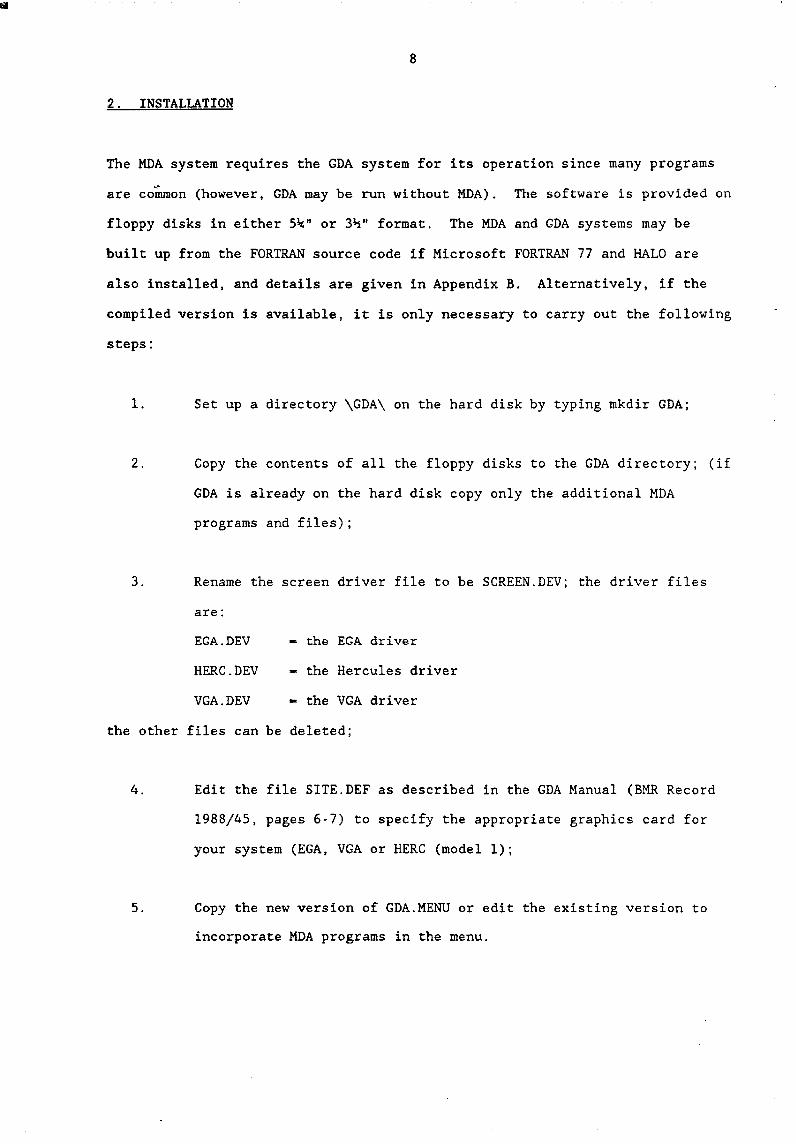
2. INSTALLATION

The MOA system requires the GOA system for its operation since many programs

are common (however, GOA may be run without MDA). The software is provided on

floppy disks in either 5~" or 3~" format. The MDA and GOA systems may be

built up from the FORTRAN source code if Microsoft FORTRAN 77 and HALO are

also installed, and details are given in Appendix B. Alternatively, if the

compiled version is available, it is only necessary to carry out the following

steps:

1. Set up a directory \GOA\ on the hard disk by typing mkdir GOA;

2. Copy the contents of all the floppy disks to the GOA directory; (if

GOA is already on the hard disk copy only the additional MOA

programs and files);

3. Rename the screen driver file to be SCREEN.OEV; the driver files

are:

EGA.DEV

HERC.OEV

VGA.DEV

- the EGA driver

- the Hercules driver

- the VGA driver

the other files can be deleted;

4. Edit the file SITE.DEF as described in the GOA Manual (BMR Record

1988/45, pages 6-7) to specify the appropriate graphics card for

your system (EGA, VGA or HERG (model 1);

5. Copy the new version of GOA.MENU or edit the existing version to

incorporate MOA programs in the menu.

9

3. DATA ENTRY

Data may be entered into the MDA system by direct transfer from the EPMA using

program PROBE, from keyboard using the ENTMIN program, or by extraction from a

database such as the BMR Oracle database.

3.1 From Microprobe

Data may be transferred direct from ASCII file output from the electron probe

microanalyser to the GDA/MDA system using program PROBE. Full details of the

ANU/BMR system are given in Appendix E.

3.2 From Keyboard (ENTMIN)

This program enables data to be entered from keyboard and is run by typing

ENTMIN or nominating the appropriate option number (15) on the menu.

The program first requires the name of the Oracle format file (e.g.,

BOWHILL.ORC).

The mineral definition file must then be entered. OXIDE.DEF (the

default option) is used for silicates and oxides, and METAL.DEF for \

metals and sulphides.

The type of data to be entered - either oxides (as in silicates and

oxide minerals) or elements (as in sulphides and metals) - must then be

specified.

The names of the oxides (or elements) to be entered must then be

listed.

Data are then entered in turn until all the oxide or element fields are

filled.

10

NOTE: If several sessions are required to enter a dataset each session should

use a different .ORC file as ENTMIN overwrites and does not append files of

the same name. Files can be concatonated by using a text editor to join them

(after appropriate edit) or by using the merge facility for GDA files under

UTIL. When merging separate files under UTIL it is important that the sample

entries have unique sample number (SAMPNO's) to avoid confusion of sample

numbers and ordering.

The following is an example of the commands and displays produced when ENTMIN

is used to input a chromite analysis. Data are entered as oxides and the

number of cations and oxygens in the ideal formula specified (3 cations per 4

oxygens in this case) to enable calculation of Fe 203 and Fe3+ contents

from stoichiometry. Input data are indicated in following scheme by bold

type.

C:\GDA>ENTMIN

ORACLE format file name [? - LIST]: BOYHILL.ORC

Mineral definitons file [? - LIST] (OXIDE.DEF): default

Enter oxides [YIN-elements] (Y): default

give names of oxides to be entered

Oxide (exit): SI02

Oxide (exit): TI02

Oxide (exit) : AL203

Oxide (exit): CR203

Oxide (exit): V203

Oxide (exit): FEO

Oxide (exit): }{NO

Oxide (exit): NIO

Oxide (exit): MGO

Oxide (exit): CAO

Oxide (exit): default

Oxides/elements processed

MGO AL203

MNO FEO

S102

NIO

CAO

Enter values for next analysis

Wt % for SI02 (zero):

Wt % for TI02 (zero):

Wt % for AL203 (zero):

Wt % for CR203 (zero):

Wt % for V203 (zero):

Wt % for FEO (zero) :

Wt % for MNO (zero):

Wt % for N10 (zero):

Wt % for MGO (zero):

Wt % for CAO (zero):

Analysis no [1-10 chars]:

Sample number [1-10 chars]:

Mineral [1-32 chars]:

Mineral description [1.32 chars]:

11

TI02 V203 CR203

.13

2.62

3.32

54.56

.07

32.68

.92

.06

5.46

.07

38

83211078

CHRmiITE

GMASS, CORE, 20 MICRON GRAIN

No cations for Fe3+ calc. [0-99] 3

Number oxygens 4.00

Analysis 83211078/38 GMASS, CORE, 20 MICRON GRAIN

wt % o - 4 ppm

MgD 5.46 0.2853 32930

A1203 3.32 0.1372 17571

5102 .13 .0046 608

CaD .07 .0026 500

Ti02 2.62 .0691 15707

V203 .07 .0020 476

Cr203 54.56 1.5122 373301

.'

MnO

Fe203

FeO

NiO

Total

Normalise oxide

Oxide to change

.92 .0273

7.63 .2014

25.81 .7567

.06 .0017

100.65 3.0000

concentrations [YIN]

(none):

38

83211078

CHROMITE

12

7125

53397

200627

472

(N)?

Analysis no

Sample no

Mineral

Description

Number oxygens

Number cations

GMASS, CORE, 20 MICRON GRAIN

4.00

3

Change values [Y/N (N)?

Accept analysis [U/N] (Y):

Enter another analysis [Y/N] (Y)?

3.3 Extraction From Oracle Database

Data may be extracted from the (Oracle) database in ASCII format. Full

details of this procedure are given on pages 8 to 11 in the GDA manual (BMR

Record 1988/45).

13

4. ORACLE

Data entered into the system in Oracle format (i.e., 80 character ASCII files)

must be converted into an internal (GDA) file for subsequent processing using

the ORACLE program.

" Data in ASCII format may be edited using a text editor (non-document mode in

YORDSTAR) prior to conversion to an internal (GDA) file. Any data can be

entered providing they are in this format, i.e., the Oracle data base does not

have to be used.

The file consists ,~ records of up to 80 characters. The first significant

records describe the fields in the file, and paired with each record is

another with ______ indicating the maximum number of characters in the

field. The actual data records follow, and must follow, the header records

format. An example is given below of an ASCII file in Oracle format.

ANALNO

SAMPNO

MINERAL

MINDESCR

STRATUNIT

OXYGENS

CATIONS

SI02

NA20

MGO

AL203

P20S

K20

CAO

T102

CR203

MNO

FEO

NIO

NA

MG

AL

SI

p

K

CA

TI

CR

MN

FE

NI

31457 WANDAGEE GARNET CONCENTRATE M97 GEN 256 GARNET 002 PIPE M97

12.00 .00

41.5310 -.0198

19.6979 18.0241

.0376 -.0122 6.9150

.1536 7.9976

.3071 7.0444 - .0354

.0000

.0000

.0000

.0000

.0000

.0000

.0000

.0000

.0000

.0000

.0000

.0000

14

15

Restrictions applying to the file are: the maximum field size for descriptive

fields is 32 characters, and for concentrations is 20 characters. Descriptive

fields that are too long are truncated. Five characters are usually enough

for concentrations but ten is preferable with the decimal point being

included. Concentrations can be given as decimal values or right-justified

integers.

analysis.

The descriptive fields must all be at the beginning of each

The field SAMPNO must be in the descriptive fields to give an

identifier for each sample (for assigning purposes, etc.). The optional field

ANALNO is usually used for mineral analyses as there are commonly several

analyses for each sample. Subsequent fields are taken as containing numerical

data. With this proviso, the actual order within each set of fields (i.e.,

descriptive and concentration) is immaterial. A concentration of zero means

that there is no value for that element. When an element concentration is

below the detection limit, the value given is the negative of the detection

limit. The value used in processing will be half the positive value. All

field names are held internally in upper case to simplify comparisons, but can

be redefined for the report programs,

The program is run by typing ORACLE or option 2 of the main GDA-MDA menu.

You must provide the name of the Oracle file to be read in (e.g., WAND.ORC).

You must also give the name of the internal file to be generated. The default

CURRENT.GDA is also the default for other programs. It is advisable to use

the same file name for the GDA file as for the Oracle file and unless

otherwise specified the standard .ORC and .GDA file extensions are applied.

Often the data file will have been transferred to the PC over a network and

there could be corrupted records due to transmission errors. There is a

choice of either having concentrations set to zero on read errors or being

asked to type in correct values.

16

5. ASSIGN

As with GDA the first processing step is to assign the samples in the GDA file

to groups. A group is a logical set of samples which will be displayed so

that all samples within it are represented by the same symbol. At least some

of the samples on a GDA file must be assigned to groups (or a single group)

before plots can be generated.

Samples are assigned to a group according to logical operations on the

descriptive fields (e.g., SAMPNO, ANALNO, MINERAL, MINERAL DESCRIPTION etc.)

on the file.

The program is run by typing ASSIGN or option 3 on the main GDA-MDA menu.

Option I on the ASSIGN menu is then selected to define the group logic. A

global selection can be specified to provide overall criteria for accepting or

rejecting samples; if no global logic is specified all samples will be

considered.

The following must be specified for each group:

The group name (maximum of 20 characters), which appears on the

legend and on menus for selection of group parameters such as the

symbol;

Logical expressions to assign the samples to the group.

The logic is typed in as lines, where each line is an 'or' condition. A

maximum of 10 lines (ie., conditions) can be specified. Each line consists of

one or more logical tests separated by 'and' conditions. The tests are given

as the descriptive field name compared to a text string. Operations are

equality

!- inequality

&& and.

.~

17

For example, different minerals can be assigned to separate groups using

MINERAL -- or different groups of the same mineral assigned to separate groups

on the basis of mineral description using MINDESC rock type using

LITHOLOGY -- , or rock unit using STRATUNIT etc.

Note that upper and lower case are taken as the same in the comparison. Both

the descriptive field name and text string can be shortened (but must be

unique) and the text comparison will be anywhere in the data field. It may be

useful to have extra information in other fields (e.g., other data) to aid

assignment of samples or analyses into groups.

After the logic ~as been specified for each group the file is processed and

the samples assigned to groups (option 12). Where the assignment criteria are

ambiguous or a sample(s) has characteristics found in more than one group it

will be assigned to the first group encountered and the other assignable

groups listed as 'group conflict'. Samples falling outside the assignment

criteria are not assigned. All samples may be assigned to one group, if

desired (option 13).

The logic and group names can be re-entered if an error has been made. Items

2-9 on the ASSIGN menu allow editing of the logic. The logic can be stored on

a file (option 10), named, and retrieved for modification and re-use. This

should always be done when samples are first assigned to groups, as subsequent

use of ASSIGN to change or edit group logic results in loss of the previous

logic. The file can be modified with a text editor or word processor, but the

number of records in the file and the header record must not be changed (i.e.,

be careful!). It is possible to set up several logic files for a given GDA

file but the samples must be reassigned if a different logic file is to be

used.

•

18

The menu is as follows:

1 Define new set of groups

2 List global logic

3 Change global logic

4 - List group titles

5 Change group titles

6 List logic for groups

7 Change logic for groups

8 Delete groups

9 Define new groups

10 Save logic file (this should be done each time new logic is

specified)

11 Restore logic from file

12 Assign analyses to groups (using the previously specified logic).

13 Assign all analyses to group 1

Q Quit

An example of a logic file (for heavy minerals in concentrate from the

Wandagee alkaline u1trabasic suite). This logic will extract all Wandagee

chromites into group 1, chromites from Wandagee pipe M97 into group 2, all

Wandagee garnets into group 3 and all Wandagee garnets excluding these from

pipe M89 into group 4.

Global logic

SAMPNO -= WANDAGEE

Group number 1

WANDAGEE CHROMITES

MINERAL ~= CHROMITE

Group number 2

PIPE M97 CHROMITES

19

MINERAL -- CHROMITE && STRATUNIT -- PIPE M97

Group number 3

WANDAGEE GARNETS

.~ MINERAL -- GARNET

Group number 4

GARNETS EX M89

MINERAL == GARNET && STRATUNIT !- PIPE M89

The assignment of samples into the specified groups may be printed out from

the file ASSIGN.PRN. Further details of assignment procedures are given in

the GDA manual.

20

6. MDAPROG

This is the main program or core of MDA. It allows data to be extracted and

plotted on various types of graph (XY, XYZ, histogram, box-whisker, etc),

Data may be extracted on the basis of oxide/element concentration, structural

formula (i.e., cations), atomic ratios or, for particular minerals such as

pyroxenes, amphiboles, spinels and garnets, as the percentage of end-member

components. Options allow printing of specialised reports for these minerals

which allocate cations, calculate end-member components, and name and/or

classify the mineral. Another option allows projection of spinel compositions

into the spinel prism.

The options are selected from the menu of the MDA program which is run by

typing MDAPROG or option 16 on the main GDA-MDA menu. A GDA file name (as

generated in the ORACLE program) must then be specified (if using a floppy

disc the drive must be specified ego A:xyz) and also the mineral definition

file, either OXIDE.DEF or METAL.DEF depending on whether the data are as oxide

or element concentrations.

The MDA menu is as follows:

Minerals

1 Extract values for typed in expressions

2 Extract structural formulae into data sets

3 Extract pyroxenes into data sets

4 Extract amphiboles into data sets

5 Extract spinels into data sets

6 Extract garnets into data sets

7 Select groups for display

8 Delete all plot files

9 Define main plot parameters

21

10 Display data sets

11 Display histograms

12 Display XY plot

13 Display triangular plot

14 Display legend

15 Display spinel prism

16 Display box-whisker plot

17 Print structural formulae report

18 Print pyroxenes report

19 Print amphiboles report

20 Print amphibole classification report

21 Print spinels report

22 Print garnets report

23 Specify a different GDA file

Q Quit

Option (1-23, Q):

In the above menu, items 1 - 16 relate to extraction from GDA files and

graphical presentation of data. The data can be displayed on screen and/or

written to a plot file (GDAl.PLT etc.) for plotting by pen plotter or laser

printer. Items 17 - 22 are programs for the calculation of structural

formulae and printing of analyses, structural formulae, cation ratios,

end-member components, and the mineral classification. In these applications

the output is to the print file MDA.PRN which may be edited by text-editor or

word processor (non-document mode) prior to printing.

For .graphical display/analysis the first step is to extract data, either the

stored oxide/element concentrations or information calculated from this, such

as cations, end-member components, cation ratios, etc., from the GDA file for

plotting. Data are extracted into data sets (up to 4) using items 1 - 6.

22

Data extracted into datasets can be plotted on various diagrams, namely

datasets display, histograms, XY plots, triangular plots, box-whisker plots,

and the reduced and oxidised spinel prism. Plot legends (i.e., symbols and

group names) may also be displayed. These options are called up using items

10 - 14 on the MDA menu. Text may be added to any plot, and some types of

plot include statistical functions such as regression lines, means, and

standard deviations, which may be displayed if required. A shortage of memory

precludes calculation of least-squares lines for MDA. Regression curves are

available, but note that these assume that there are no errors in the X-axis

variable, i.e .• X is the independent variable and Y the dependent variable.

Normally, plots are intially displayed on the PC screen to allow inspection

and editing before being written to metafiles for later output to a plotter

using the PLOT program. Examples of the various plots available are shown

below in the relevant sections.

6.1 Extract Values for Typed in Expressions

This option is used to extract oxide or element abundances and other

information such as stratigraphic height or isotopic composition stored in the

specified GDA file and any derived values formed by arithmetic combination of

the oxide/element concentrations or other numerical data stored. It does not

enable extraction of cations from structural formulae (options 2 - 6 apply).

Operators are:

+ addition

subtraction

* multiplication

/ division

> greater than or equal to

< less than or equal to

** power

23

Functions available are:

LOGlO common logarithm

LOG natural logarithm

SQRT square root

ABS absolute value

EXP exponential

AINT truncation

TAN tangent

ATAN arc tangent

SIN sine

COS cosine

SINH hyperbolic sine

COSH hyperbolic cosine

Pi is referred to as PI. Expressions are evaluated left to right, * and /

before + and -

ambiguities.

Parentheses should be used to ensure there are no

Datasets are referred to by two character strings '$n' (e.g., $2 is dataset

number 2). Hence, datasets can be used to hold intermediate values.

The following example extracts from a set of chromite analyses the Cr203

and MgO contents (data sets 1 and 2), the A1 203 + Fe203 content (data

set 3) and Cr203 values for chromites with more than 56% Cr203

(dataset 4).

Entered responses are in bold type.

Type arithmetic expression [?-help] (Exit)

: CR203

Data set number [1 - 4]: 1

24

Type arithmetic expression [?-help] (Exit)

: MGO

Data set number [1 4 ]: 2

Type arithmetic expression [?-help] (Exit)

: AL203 + Fe203

Data set number [1 - 4]: 3

Type arithmetic expression [?-help] (Exit)

: CR203 > 56

Data set number [1 - 4]: 4

These datasets can be displayed using option 10 (- Display data sets) followed

by the DATA SET sub-menu options 1 and 2. Datasets selected are used as the X

axis.

A help file is available by returning ?

The help file also lists the oxides and element names held in the GDA file

which can be extracted.

Derived values are formed from arithmetic combinations of element or oxide

concentrations. Components are identified by name.

An example is:

(FE203 + FEO)/2 > 50 < 90.0

This creates a new concentration which is half the sum of the concentrations

of the individual components (in this case oxides). Any valid arithmetic

expression is permitted but only values in the given range are accepted.

Previously calculated values held in other datasets can be referenced by using

the two characters $n, where n is the dataset number. This enables holding of

intermediate values in datasets. Press Enter to continue.

"

25

6.2 Extract Structural Formulae into Datasets

This option is used to extract cations (or any arithmetic combination of

cations) calculated from the oxide and elemental concentrations in the GDA

file. The program calculates structural formulae on the basis of the number

of cations and oxygens specified in the GDA file. An option is available to

specify calculation with or without ferric iron.

The following is an example of the type of cation ratios commonly used in

plotting of chromian spinels.

Type arithmetic expression [?-help] (Exit)

: lOO*Cr/(Cr+Al)

Data set number [1 - 4]: 1

Type arithmetic expression [?=help] (Exit)

: lOO*Mg/(Mg+Fe2+)

Data set number [1 - 4]: 2

Type arithmetic expression [?-help] (Exit)

: Fe3+/(Cr+Al+Fe3+)

Data set number [1 - 4]: 3

Type arithmetic expression [?-help] (Exit)

: Cr/(Cr+Al+Fe3+)

Data set number [1 - 4]: 4

Calculate Ferric [YIN] (N)? Y

The calculation of ferric takes slightly longer to perform than the standard

structural formula.

26

Atomic ratios such as lOOK/(K+Na+Ca) i.e., Or content, can be extracted and

stored and later renamed to 'Mol percent Or' or similar using options provided

under the plotting routines.

Extraction of combined oxide or elemental weight percent data or other

parameters such as stratigraphic height or with structural formulae components

can be made by sequential extraction using options 1 and 2 and storing the

data as datasets 1-4. Data from previous extractions will be held in their

designated datasets until overwritten by subsequent extractions or exit from

the MDAPROG program.

6.3 Extract Pyroxenes into Datasets

This option extracts pyroxenes and calculates structural formulae on the basis

f 6 . F 3+. . h· (4· o oxygen atoms, estlmates e assumlng pyroxene st01C lometry catlons

per 6 oxygen atoms), assigns cations to the various pyroxene sites (T, M1 and

M2) and calculates In activity Mg2Si20 6 , following the method of Wood

and Banno (1973).

Atomic ratios are calculated as follows:

Mg# 2+ lOOMg/(Mg+Fe )

Ca* lOOCa/(Ca+Mg+Fe)

Mg* IOOMg/(Ca+Mg+Fe)

Fe* IOOFe/(Ca+Mg+Fe)

wo .. IOOWo/(Wo+En+Fs)

EN" lOOEn/(Wo+En+Fs)

FS" lOOFs/(Wo+En+Fs)

ACF2 - Al (MI)+Cr+Fe3++2Ti

In(a)En - log activity enstatite

Wo, En and Fs are calculated after the other end-members in the order given

below.

27

The program alo calculates the molecular percentage of the end members:

NaCrSi206 (Ureyite) Ur '. CaCr2Si06 (Ca-Cr-tschermaks) CaCrTs

NaAlS1206 (Jadeite) Jd

NaFe 3+Si2

06 (Acmite) Ac

CaTiA1206 (Ca-Ti-tschermaks) CaTiTs

CaA12Si06 (Ca-tschermaks) CaTs

caFe3+2Si0

6 (Ca-ferritschermaks) CaFeTs

CaSi03 (Wollastonite) Wo

MgSi03 (Enstatite) En

FeSi03 (Ferrosili te) Fs

End-members are calculated in the order listed following the method of

Cawthorn and Collerson (1974), except that the Cr pyroxene components ureyite

and Ca-Cr-tschermaks are calculated before jadeite.

The full list of cations, site allocations, atomic percentages and molecular

percentages of end-members, displayed under [?J help, is:

Si Ti Al Cr Fe3+ Fe2+ Mn

Ni Mg Ca Na K Sum AI/2

Al(T) Al(Ml) Mg(Ml) (ACF2T) T(tot) Ml(tot) M2(tot)

In(a)EN mg# Ca* Mg* Fe* WO" EN"

FS" Ur CaCrTs Ac Jd CaTiTs CaTs

CaFeTs Wo En Fs

This can be viewed by selecting the help option (?) when asked to type

arithmetic expression. Derived values may be formed by any arithmetic

combination of the above values.

28

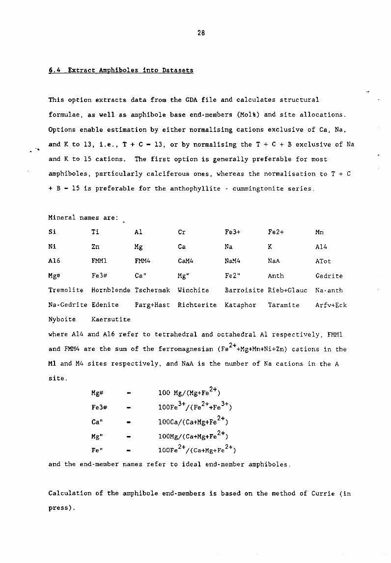
6.4 Extract Amphiboles into Datasets

This option extracts data from the GDA file and calculates structural

formulae, as well as amphibole base end-members (Mo1%) and site allocations.

Options enable estimation by either normalising cations exclusive of Ca, Na,

and K to 13, i.e., T + C - 13, or by normalising the T + C + B exclusive of Na

and K to 15 cations. The first option is generally preferable for most

amphiboles, particularly calciferous ones, whereas the normalisation to T + C

+ B - 15 is preferable for the anthophyllite - cummingtonite series.

Mineral names are:

Si Ti A1 Cr Fe3+ Fe2+ Mn

Ni Zn Mg Ca Na K Al4

A16 FMMI FMM4 CaM4 NaM4 NaA ATot

Mg# Fe3# Ca" Mg" Fe2" Anth Gedrite

Tremolite Hornblende Tschermak Winchite Barroisite Rieb+Glauc Na-anth

Na-Gedrite Edenite Parg+Hast Richterite Kataphor Taramite Arfv+Eck

Nyboite Kaersutite

where Al4 and A16 refer to tetrahedral and octahedral Al respectively, FMI'11

and FMM4 are the sum of the ferromagnesian (Fe 2++Mg+Mn+Ni+Zn) cations in the

MI and M4 sites respectively, and NaA is the number of Na cations in the A

site.

Mg# 2+ 100 Mg/(Mg+Fe )

Fe3# 100Fe3+/(Fe2++Fe 3+)

Ca" 2+ lOOCa/(Ca+Mg+Fe )

Mg" 2+ lOOMg/(Ca+Mg+Fe )

Fe" 2+ 2+ lOOFe /(Ca+Mg+Fe )

and the end-member names refer to ideal end-member amphiboles.

Calculation of the amphibole end-members is based on the method of Currie (in

press) .

.,

...

29

Amphiboles have the general formula Al_2B2CSTS022(OH,Cl,F)2 where

2+ C M F 2+ M 1 F 3+ Tl· A - Na. K; B - Na, Li, Ca, Mn, Mg, Fe ; - g, e , n, A, e ,

; T - Si, Al with other less common substitutions. The A, Band T-sites are

used to classify 17 end-member molecules (Hawthorne, 19S3). Amphibole

end-members are first classified into A-site empty and A-site full types.

End-members are then calculated according to Si6 , Si7 and SiS and B-site

occupancy with the B-site filled by FM, Ca or Na or mixed Na-Ca cations.

6.5 Extract Spinels into Datasets

In this option spinels are extracted and their structural formulae are

calculated on the basis of 4 oxygen atoms. Ideal end-member spinels are also

calculated in the order listed following a modified version of the method of

Mitchell and Clarke (1976). An option allows calculation of ferric iron

assuming stoichiometry (i.e., 3 cations per 4 oxygens) depending on whether

the oxidised or reduced spinel prism is selected.

For the oxidised prism the program calculates the following components (viewed

using the help option).

Mineral names are:

Mg# AI/TriV Cr/TriV Fe3+/TriV Cr/(Cr+AI) SI TI

AL CR FE3+ FE2+ MN MG NB

V NI ZN CA ZnA1204 MgAI204 FeA1204

MnA1204 Mg2Ti04 Mn2Ti04 Fe2Ti04 MgCr204 FeCr204 MnCr204

Fe304

where TriV - the sum of the trivalent cations AI, Cr and Fe3+.

30

For the reduced spinel prism the following components are calculated.

Mineral names are:

Mg# Al/TriV Cr/TriV Fe3+/TriV Cr/(Cr+Al) SI TI

AL CR FE3+ FE2+ MN MG NB .":"

V N1 ZN CA ZnA1204 MgA1204 FeA1204

MnA1204 Mg2Ti04 Mn2Ti04 Fe2Ti04 MgCr204 FeCr204 MnCr204

Fe304

6.6 Extract Garnets into Datasets

This option allows garnet data to be extracted and structural formulae

calculated on the basis of 12 oxygen atoms. An option allows calculation of

ferric iron assuming stoichiometry (8 cations per 12 oxygens). Selection can

be made from concentration data, cations, cations in various sites, and

end-member garnet molecules as shown in the listing below (viewed using the

help option).

Mineral names are:

P20S Zr02 Si02 Ti02 A1203 Cr203 V203

Y203 Fe203 FeO MnO NiO MgO CaO

Na20 Total P Zr Si Ti Al

Cr V Y Fe3+ Fe2+ Mn Ni

Mg Ca Na Sum Ca* Mg* Fe*

MgNo# MgNo SiTET AlTET TiTET Fe3+TET SUM

SiY AIY Fe3Y TiY Y -Site X-Site Maj

Yt Ya Gold Kimz Fe-Kimz Uvar Knor

Sch And Py Sp Gr AIm Koh

Ski Cal B1y

Calculation of the garnet end-members is modified from the method of Rickwood

(1968) to include majorite (maj). The full names and formulae of the

2+ end-members are given in 6.21. MgNo# and MgNo refer to 100Mg/(Mg+Fe )

31

calculated with FeD only and all Fe as FeD, respectively. Ca*, Mg* and Fe* -

2+ 100 Ca/(Ca+Mg+Fe ), etc.

6.7 Select Groups for Display

This item allows selection of individual groups of samples within the data

file.

Each of the groups is displayed in turn and selection is by responding yes or

no.

6.8 Delete all Plot Files

All existing plot files (GDAI.PLT etc.), are deleted by this function. Care

should be taken to ensure that a back-up copy is made of those plot files

required for future plotting (replotting).

6.9 Defining Plot Parameters

Item 9 on the MDA menu ('Define main plot parameters') is used to allocate

symbols, pen colours, and linetypes to sample groups, and to define symbol,

text, and axis dimensions. Commonly the default parameters may be adequate,

but these may be changed and the plot parameters stored on a file for

subsequent retrieval and re-use. Different parameters may be required for

display on screens and on plotters.

The various optional parameters can be allocated using the following menu.

Default values are given in brackets.

MAIN PLOT PARAMETERS

1 - Retrieve plot parameters (from file)

2 Change title text height (I. Scm)

3 - Change axes labels text height (l.Ocm)

32

4 - Change sample numbers and points text height

5 - Change symbol height (0.5cm)

6 - Change axes tick height (1.0cm)

7 - Change font (0.5)

8 - Change group pens

9 Change group symbols

10 - Change group 1inetypes (1)

11 - Change axes pen (1)

12 c Change titles pen (1)

13 - Change histogram pen (1)

14 = Change plot title

15 = Change legend symbol and text heights (1.0)

16 - Change axes lengths (X - 25.0cm; Y - 20.0cm)

17 Define metapath & preceeding characters in name

18 - Store plot parameters (on file)

Option [1 - 17] (Exit):

An example of a plot parameters file is given on pages 21-22 in the GDA

manual. Normally the format will not be of interest to the user as it will

not be necessary to edit such a file.

There are choices of up to 8 pens (depending on the type of plotter), 15

symbols, 6 1inetypes and 19 fonts, all of which may be displayed on screen by

selecting the display option (?). As default values for these, pen 1 and

symbol 1 are assigned to group I, pen 2 and symbol 2 to group 2, and so on.

Pens and symbols assigned to each group may be checked by displaying the

legend. The default linetype for all groups is 1 (solid line); note that the

linetypes as displayed on the screen are slightly different from those used by

the plotter (they are defined in the graphics package).

The symbols, linetypes and fonts are shown in Figures 1-4 in the GDA manual.

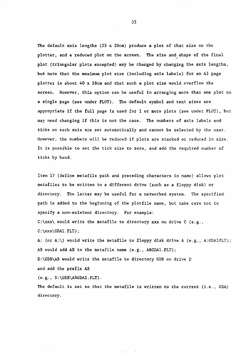
33

The default axis lengths (25 x 20cm) produce a plot of that size on the

plotter, and a reduced plot on the screen. The size and shape of the final ~

plot (triangular plots excepted) may be changed by changing the axis lengths,

but note that the maximum plot size (including axis labels) for an A3 page

plotter is about 40 x 28cm and that such a plot size would overflow the

screen. However, this option can be useful in arranging more than one plot on

a single page (see under PLOT). The default symbol and text sizes are

appropriate if the full page is used for I or more plots (see under PLOT), but

may need changing if this is not the case. The numbers of axis labels and

ticks on each axis are set automatically and cannot be selected by the user.

However, the numbers will be reduced if plots are stacked or reduced in size.

It is possible to set the tick size to zero, and add the required number of

ticks by hand.

Item 17 (define metafile path and preceding characters in name) allows plot

metafiles to be written to a different drive (such as a floppy disk) or

directory. The latter may be useful for a networked system. The specified

path is added to the beginning of the plotfile name, but take care not to

specify a non-existent directory. For example:

C:\xxx\ would write the metafile to directory xxx on drive C (e.g.,

C:\xxx\GDAl.PLT);

A: (or A:\) would write the metafile to floppy disk drive A (e.g., A:GDAIPLT);

AB would add AB to the metafile name (e.g., ABGDAl.PLT);

D:\GDB\AB would write the metafile to directory GDB on drive D

and add the prefix AB

(e.g., D:\GDB\ABGDAl.PLT).

The default is set so that the metafile is written to the current (i.e., GDA)

directory.

34

6.10 Display Datasets

This option enables one or more datasets to be displayed ~U an XY plot of

value against sample order in the dataset. Each sample group is displayed

sequentially, using the appropriate symbol and pen colour. Either a single

dataset (e.g., element) may be displayed, or plots of up to 4 datasets may be

stacked.

The menu is as follows:

1 Display (either on screen or metafile; plot number (1-99) must be

specified in latter case)

2 Select datasets (e.g., elements) for display (if more than one is

selected, plots will be stacked)

3 Change plot title

4 Change axes titles (for any selected dataset)

5 Display sample numbers (on plot)

6 Set axes extremes to data range plus 20%

7 Set axes extremes to nice limits (this is the default which selects a

logical whole-number range for each axis, depending on which groups

are selected for display)

8 Set axes extremes to typed-in values (any values may be selected, but

note that they will also apply to histograms and XY plots (but not

triangular plots»

9 Set log or linear axes (for any selected dataset)

10 Define pen for mean lines (0): (1 of up to 8 colours; displays mean

for all groups selected for display in 13)

11 Define pen for median lines (0) (as 10)

12 Define pen for standard deviation lines (0)(as 10)

13 Select groups to be displayed (any or all assigned groups may be

displayed on each plot)

35

14 Specify additional plot points and/or text

Additional plot points or text such as a legend, may be added to

previously selected plots via the keyboard. The following must be

given:

1. X, Y co-ordinates (separated by a comma; previously specified

points or text will be deleted if no values are entered here;

co-ordinates outside the plotting area are permissible).

2. Pen number.

3. Symbol number (if none is given, only text will be output).

4. Text (e.g., sample number or a legend; 0 . 50 characters).

5. Y-axis dataset (this number must be specified for each

extra point or text required; for stacked plots, points or

text may be added to any plot by specifying the appropriate

dataset).

Note that the given XY co-ordinates define the centre of the symbol

or, if no symbol is specified, the bottom of the first character of

text. All added points or text required for a given plot (either

single or stacked) must be specified in one operation (as

previously added points will be replaced when this option (14) is

selected a second time); the maximum is 20 extra points and/or text

lines).

15 List statistics (includes minimum, maximum, mean, median, standard

deviation, skewness, and kurtosis; calculated for all samples in the

selected groups and for selected datasets; if log axes are selected,

statistics will be calculated using natural log values).

The statistics are displayed, and are also listed on a file MDA.PRN,

which may subsequently be printed (or edited if required)

36

6.11 Display Histograms

Histograms of three types may be displayed - for single datasets, stacked for •

up to 4 datasets, or stacked for selected groups for a single dataset (see

item 13). The menu is similar to that for display of datasets:

1 Display (on screen or metafile 1-99)

2 Select datasets (e.g., elements for display)

3 Change plot title

4 Change axes titles

5 Set axes extremes to data range plus 20%

6 Set axes extremes to nice limits

7 Set axes extremes to typed-in values

B Define histogram box width

9 Define pen for mean lines

10 Define pen for median lines

11 Define pen for standard deviation lines

12 Select groups to be displayed

13 Select histogram type

1. Single element (for selected groups)

2. Stacked for selected datasets (for all selected groups)

3. Stacked groups for one dataset (each selected group is plotted

separately with group numbers at right)

14 Specify additional plot points and/or text (for histograms, this

option is mainly useful for adding text, such as a legend, to a

previously selected plot:

1. X, Y co-ordinates (separated by a comma; if no values are entered,

previously specified points or text will be deleted)

2. Pen number

3. Symbol number (if none is given, only text will be output)

4. Text (e.g .• a legend; 0 - 50 characters)

5. Y-axis dataset (this specifies the dataset selected for a single

'"

37

histogram (actually the X-axis in this case), or for any dataset

on a stacked plot of datasets)

Group number (this specifies the group for a stacked plot of

groups for one dataset)

Note: the given XY co-ordinates define the centre of the symbol or, if

no symbol is specified, the bottom of the first character of text.

The maximum number of added points and/or text lines is 20. All those

required for a given plot (either single or stacked) must be specified

in one operation).

15 List statistics (for all samples in the selected groups and for

selected d:.; asets; may be printed from file MDA. PRN) .

An example of a histogram used to portray garnet compositions from two of the

Wandagee alkaline u1trabasic pipes in Figure 1.

FIG. 1. STACKED HISTOGRAM OF GARNET COMPOSITIONS

~ ~

• I • I • I • I • I -~ -...., 8

~ ----

0 4 0 ()

--~ -~ -~

I I • I • I • I • I -~

• I • I I I I I • I I- -

...., 20 --~ -

~ -0 0') 10 ~

~ -~ -~ --l- I I • I I I • I • I -

~ l-I I • I • I I I • I -

....., 12 ~

--~ -~ -

n 8 0 4 N

---I- ---I.- -() -- I • I • I I I I I -

4 8 Frequency

39

6.12 Display XY Plot

As for datasets and histograms, plots may be single or stacked. Menu items 1 .~

- 12 are identical to the display dataset menu. Because of memory limitations

options 13 and 19 on the GDA menu - least squares line fitting and least

squares lines for individual groups - are not available for MDA. The

remainder are as follows:

14 Define pen for regression polygons (different colours may be specified

for 1st, 2nd and 3rd order regressions, calculated for all selected

groups, using either values or log values)

15 Select groups to be displayed

16 Specify additional plot points and/or text (additional points or text,

such as a legend, may be added to previously selected plots via the

keyboard

1. X, Y co-ordinates (separated by a comma; previously specified

points or text will be deleted if no values are entered here)

2. Pen number

3. Symbol number (if none given, only text will be output)

4. Text (e.g., sample number or a legend; 0 - 50 characters)

5. Y-axis dataset (this must be specified for each extra point or

text required; for stacked plots, points or text may be added to

any plot by specifying the appropriate dataset).

Note: the given XY co-ordinates define the centre of the symbols

or, if no symbol is specified, the bottom of the first character

of the text. If a new X-axis dataset is selected the added points

may still appear, so be sure to delete any additional points (by

choosing option 16 again, but not entering any XY co-ordinates)

before selecting new datasets for display. All added points or

text required for a given plot (either single or stacked) must be

specified in one operation; the maximum number of added points

and/or text lines is 20).

" ..

40

17 Specify graphics overlay files (lines and/or text may be added by

selecting an appropriate file - see appendix D for details of format

and available files; make sure that the X."and Y datasets are correct

and the axis extremes are appropriate; the Y-axis dataset and name of

the graphics overlay file (????GRF) must be given)

18 Regression curves for individual groups (as 14, except that curves are

calculated separately for each displayed group)

20 List statistics (comprises minimum, maximum, mean, median, standard

deviation, skewness, kurtosis, correlation coefficient, and 1st 2nd

and 3rd order regression coefficients, standard deviations, and

T-values; calculated for all samples in the selected groups and for

selected datasets or pairs of datasets (X with each Y); if log axes

are selected for any dataset(s), statistics will be calculated using

the natural logarithms of those dataset values; if regression curves

for individual groups are specified (18), statistics for each selected

group will also be listed; results may be printed from file MDA.PRN)

An example of an XY plot showing the composition of diamond facies

chrome spinels is shown in Figure 2 and the corresponding statistics

printout is given in Table 1.

r

f )

.~

41

TABLE 1. STATISTICAL DATA FOR FIGURE 2.

XY PLOT OF DIAMOND FACIES CHROMITES

lOOMg/(Mg+Fe2+)

Minimum: Maximum: Mean: Median Standard Deviation: Skewness: Kurtosis :

lOOCr/(Cr+Al)

Minimum: Maximum: Mean: Median Standard Deviation: Skewness: Kurtosis:

Regression Statistics:

2.8740 79.4540 60.6240 62.6530 14.8066 -1. 8929 5.4445

82.8660 95.7810 89.0946 88.7500

2.8370 .4491 .3798

Independent Variable: 100Mg/(Mg+Fe2+) Dependent Variable: 100Cr/(Cr+A1)

Correlation Coefficient: -.5204 Product-Moment Correlation Coefficient based on 61 pairs of values: -.5204

Polynomial of degree 1 Standard error: 2.4 Regression Coefficient(s): 95.14 Coefficient(s) Standard Deviation: .2130E-01

- .9972E-Ol

T-Value (s) : -4.682

Polynomial of degree 2 Standard Regression Coefficient(s): Coefficient(s) Standard Deviation: T-Value(s):

Polynomial of degree 3 Standard Regression Coefficient(s): Coefficient(s) Standard Deviation: T-Value(s):

error: 2.4 92.92 .1701E-Ol-.1249E-02 .7103E-01 .7262E-03 .2396 -1. 720

error: 91.45 .2437 1.473

2.4 .3589 -.1103E-01 .6711E-02 .5009E-04

-1. 643 1. 465

.7340E-04

FIG. 2. XY PLOT OF DIAMOND FACIES CHROMrrES

If6AA , . 90 • . ~ ..

4t • It~.t ~ A .-

$ 80 '-() ,... '-"

N

"'-'-() 70 .Chromite inclusions • diamond 0 In 0 ......

60 A Chromite-diamond intergrowths

20 40 60 80 100Mg/ (Mg+F e2+ )

43

6.13 Display Triangular Plot

Any 3 datasets may be selected for display on a triangular plot.

1 Display (on screen or metafile 1 - 99)

2 Select datasets (e.g., elements) for display

3 Change plot title (previous title is deleted if nothing is entered)

4 Change apex titles

5 Display sample numbers

6 Select groups to be displayed

7 Specify additional plot points and/or text (additional plot points or

text, such as a legend, may be added to previously selected plots via

the keyboard; the following must be given:

1 . X, Y, Z co-ordinates (separated by commas; either straight

element concentrations or normalised co-ordinates (i.e.,

totalling to 100) may be used; pr~iously specified points or

text will be deleted if no values are entered here; co-ordinates

outside the plotting areas (i.e., negative) are permissible, but

obviously must be adjacent to the plot)

2. Pen number

3, Symbol number (if none is given, only text will be output)

4. Text (e.g., sample number or a legend; 0 - 50 characters)

Note that the given XYZ co-ordinates define the centre of the symbol

or, if no symbol is specified, the bottom of the first character of

text. All added points or text required for a given plot must be

specified in one operation; the maximum number of added points and/or

text lines is 20. To align 2 or more lines of text vertically - for

each unit decrease in the Y co-ordinate, increase X and Z by 0.5

each).

8 Specify graphics overlay files (xxx.GRF)

An example of an XYZ plot showing the composition of garnets from two of the

Wanda gee alkaline ultrabasic pipes is given in Figure 3.

. ~

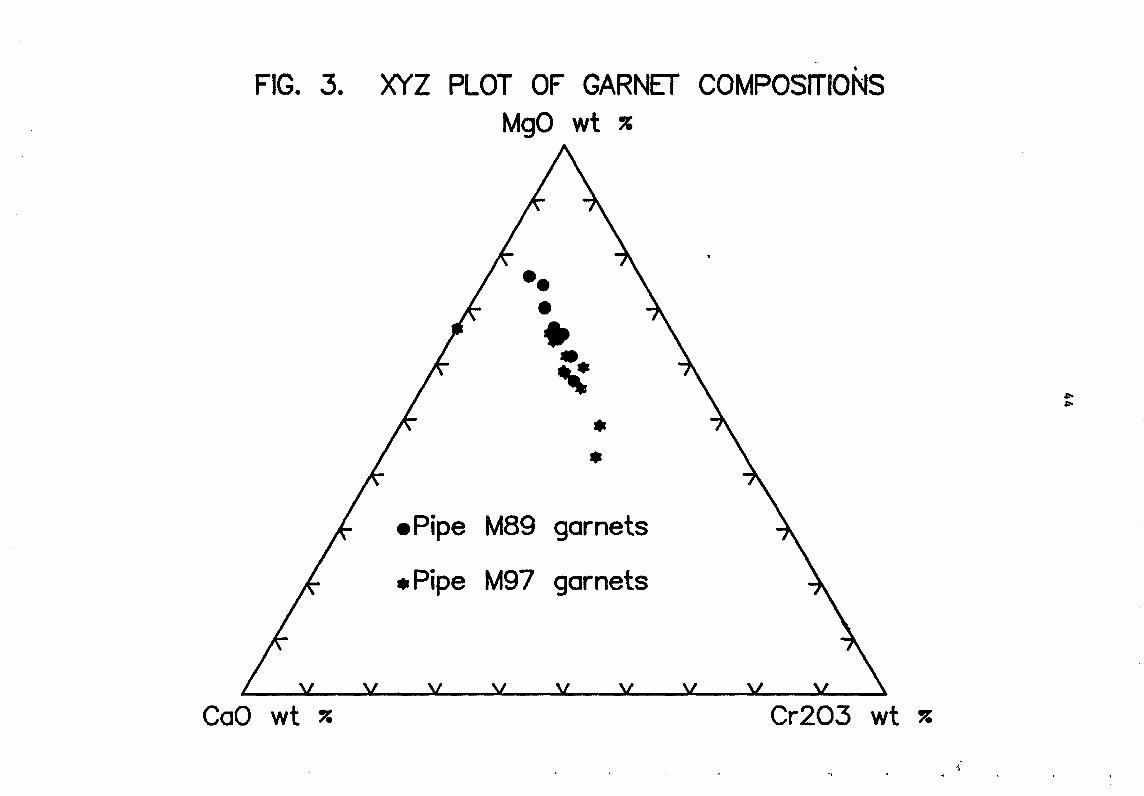
• FIG. 3. XYZ PLOT OF GARNET COMPOSITIONS

CaO wt x

MgO wt "

•• • • -. ..;

• •

• Pipe M89 garnets

• Pipe M97 garnets

Cr203 wt x

45

6.14 Display Legend

This may be used to display the symbols and the pen colours assigned to sample

groups. It may be written to a metafile so that the legend may be output to a

plotter.

6.15 Display Spinel Prism

This option allows spinel compositions to be plotted in the spinel prism

(Irvine, 1965). Projections can be made into either the oxidised prism in

terms of (MgFe)A1204-(MgFe)cr204-(MgFe)Fe204 with Fe3+

calculated from stoichiometry or the reduced prism in terms of

(MgFe)A1204-(MgFe)Cr204-(MgFe)2Ti04 with all Fe assumed to be

Fe 2+.

The submenu is

SPINEL PRISM

1 = Display (on screen or metafile 1-99)

2 - Change plot title

3 = Display sample numbers

4 - Select groups to be displayed

Example of the spinel prism plots for both the oxidising and reduced prisms is

shown in Figures 4a,b.

FIG. 4A. OXIDISED SPINEL PRISM PLOT Fe304

MgFe204

-" ~...... •• e • ........... .....

MgCr204

FeCr204

FIG. 48. REDUCED SPINEL PRISM PLOT

0.8

MgAI204 o

Fe2Ti04

MgCr204

"~

FeCr204

48

6.16. Box-Whisker Plot

Box-whisker plots may be used to,pisplay many datasets on a single diagram

together with mean and standard deviation boxes for each dataset. Such plots

are useful for highlighting anomalous values and for making comparisons with

average data. The box-whisker menu is:

BOX-WHISKER PLOT

1 Display

2 Change plot title

3 Set axes extremes to data range plus 20%

4 Set axes extremes to nice limits

5 Set axes extremes to typed in values

6 Select groups to be displayed

7 Select box-whisker type

8 Specify additional plot points and/or text

9 Specify box size

10 Display box

11 Display samples inside box

12 Linear / log axis

13 Define pen for box

Option [1-13] (Exit):

Options 1-8 are similar to the options available for histogram plots. Option

9 is used to specify box size (0-5 standard deviations above and below the

mean; fault is 1.0). Option 10 enables the boxes to be omitted if desired,

with option 11 the sample points inside boxes may be omitted, option 12

defines linear or log axes, and option 13 offers a choice of pen colours for

the box.

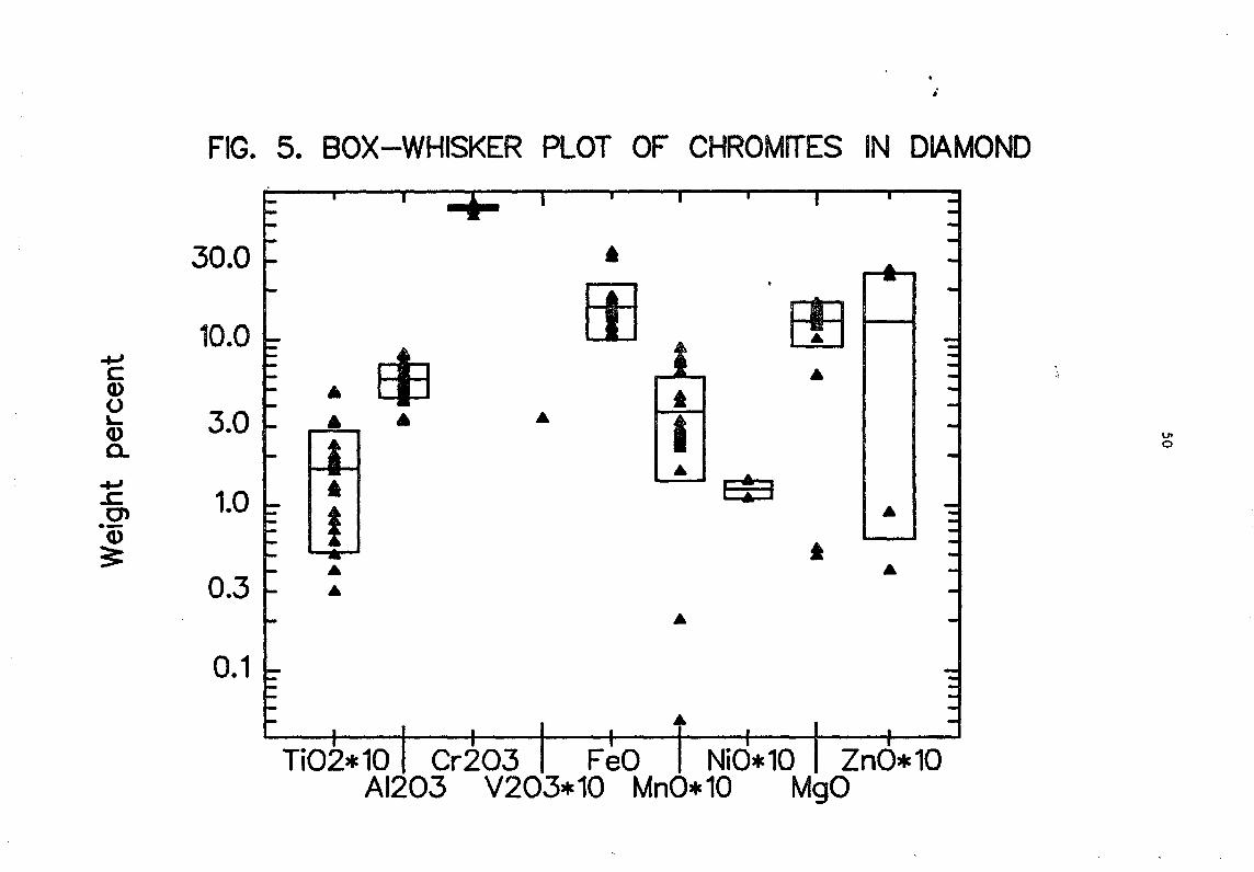
The default Box-whisker Plot Definition File (BOXWHISK.DEF) comprises the

major oxides. Suitable mineral reference files may be set up and expressions

49

as well as concentrations incorporated as required. An example of the

box-whisker plot to show compositional variation amongst chrome spinel

inclusion in diamond is shown in Fig. 5 . . ~

i

FIG. 5. BOX -WHISKER PLOT OF CHROMITES IN DIAMOND

30.0 • .... -ffi ffi 10.0

...... EIJ c • ., Q) ... t 0 L. 3.0 A A I Q) UI

Q. 0

• ...... A .r:::. 1.0 (1) I --Q)

3: • • 0.3 •

0.1

51

6.17. Print Structural formulae Report

~

This option generates on file MDA.PRN a table of analyses and atomic

proportions calculated using the number of oxygens and cations stored in the

GDA data file. Ferric iron will only be calculated if a non-zero value value

is held in the cations field. The sample number, analysis number and mineral

description fields are printed at the bottom of the table. An example is

given in Table 2. The file MDA.PRN may be modified using a text-editor prior

to printing.

' ..

52

TABLE 2. EXAMPLE OF STRUCTURAL FORMULAE REPORT

~.

STRUCTURAL FORMULAE - crnod.GDA

A MgO 12.82 A1203 7.88 Si02 .06 CaO <.02 Ti02 .10 V203 .17 Cr203 64.68 MnO .16 Fe203 .54 FeO 13.60 NiO .07 ZnO .11 Total 100.18

Ox 4.0000 Mg .6241 Al .3033 Si .0020 Ti .0025 V .0045 Cr 1. 6702 Mn .0044 Fe+++ .0132 Fe++ .3714 Ni .0018 Zn .0027 Total 3.0000

A: AR2/1 B: N38/1 C: N41/1 D: N45/1 E: N45/2

B 15.42 14.02 <.02 <.02

.11

.00 57.49

.12 2.84

10.80 .13

. .00 100.93

4.0000 .7151 .5141

.0026

1.4142 .0032 .0666 .2811 .0033

3.0000

C D E 14.84 14.70 14.72 14.27 13.60 10.40

.03 .03 <.02 <.02 <.02 <.02

.20 .21 1. 73

.30 .28 .23 57.59 57.63 57.53

.12 .09 .14 1. 05 l. 56 3.00

11.61 11.62 12.46 .10 .14 .19 .06 .07 .09

100.17 99.94 100.49

Atomic Proportions.

4.0000 4.0000 4.0000 .6940 .6915 .6989 .5277 .5059 .3904 .0009 .0009 .0047 .0050 .0414 .0075 .0071 .0059

1.4287 1.4381 1.4488 .0032 .0024 .0038 .0248 .0371 .0720 .3045 .3068 .3318 .0025 .0036 .0049 .0014 .0016 .0021

3.0000 3.0000 3.0000

- AVERAGE 8 CHROMITE CORES - CHROMITE CORE - AVERAGE 8 CHROMITE CORES - AVERAGE 14 CHROMITE CORES co CHROMITE RIM

53

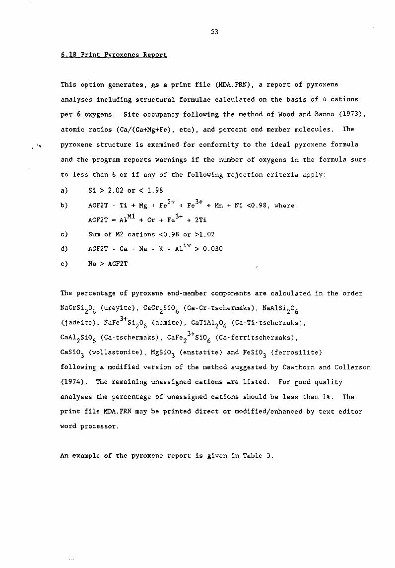
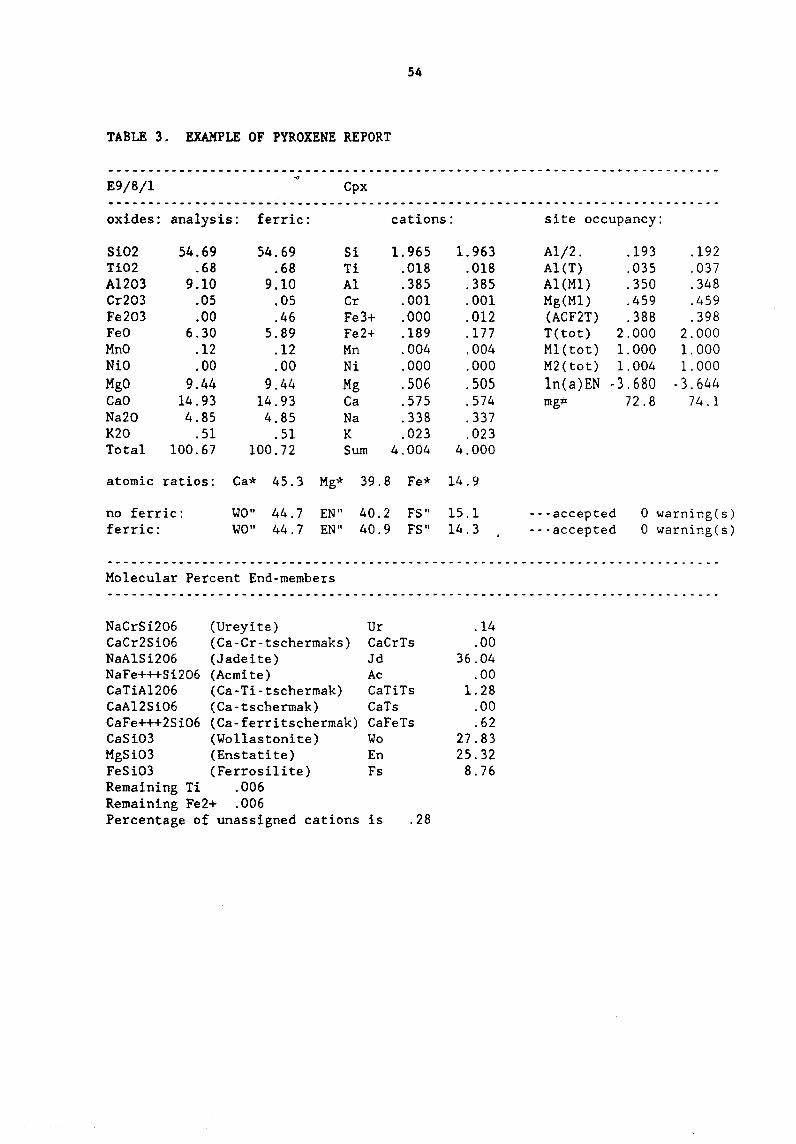
6.18 Print Pyroxenes Report

This option generates, .as a print file (MDA.PRN), a report of pyroxene

analyses including structural formulae calculated on the basis of 4 cations

per 6 oxygens. Site occupancy following the method of Wood and Banno (1973),

atomic ratios (Ca/(Ca+Mg+Fe), etc), and percent end member molecules. The

" pyroxene structure is examined for conformity to the ideal pyroxene formula

and the program reports warnings if the number of oxygens in the formula sums

to less than 6 or if any of the following rejection criteria apply:

a) Si > 2.02 or < 1.98

b) ACF2T - Ti + Mg + Fe2+ + Fe3+ + Mn + Ni <0.98, where

ACF2T = A1M1 + Cr + Fe3+ + 2Ti

c) Sum of M2 cations <0.98 or >1.02

d) ACF2T - Ca - Na - K - A1iv > 0.030

e) Na > ACF2T

The percentage of pyroxene end-member components are calculated in the order

NaCrSi 206 (ureyite), CaCr2Si06 (Ca-Cr-tschermaks), NaA1Si206 (jadeite), NaFe 3+Si206 (acmite), CaTiA1206 (Ca-Ti-tschermaks),

CaA1 2Si06 (Ca-tschermaks), caFe23+Si06 (Ca-ferritschermaks),

CaSi03 (wollastonite), MgSi03 (enstatite) and FeSi03 (ferrosilite)

following a modified version of the method suggested by Cawthorn and Collerson

(1974). The remaining unassigned cations are listed. For good quality

analyses the percentage of unassigned cations should be less than 1%. The

print file MDA.PRN may be printed direct or modified/enhanced by text editor

word processor.

An example of the pyroxene report is given in Table 3.

54

TABLE 3. EXAMPLE OF PYROXENE REPORT

-------------------------------------------------------- ... _-------------------."

E9/8/1 Cpx ---_ ... -.----- ... -_ ..... -----_ ...... _----.-------- ... _--------- ... ----- ... -------------- .. ---_ ...

oxides: analysis: ferric: cations: site occupancy:

Si02 54.69 54.69 Si 1. 965 1. 963 Al/2. .193 .192 Ti02 .68 .68 Ti .018 .018 A1(T) .035 .037 A1203 9.10 9.10 Al .385 .385 Al (M1) .350 .348 Cr203 .05 .05 Cr .001 .001 Mg(M1) .459 .459 Fe203 .00 .46 Fe3+ .000 .012 (ACF2T) .388 .398 FeD 6.30 5.89 Fe2+ .189 .177 T(tot) 2.000 2.000 MnO .12 .12 Mn .004 .004 M1(tot) 1.000 1.000 NiO .00 .00 Ni .000 .000 M2(tot) 1.004 1.000 MgO 9.44 9.44 Mg .506 .505 In(a)EN -3.680 -3.644 CaO 14.93 14.93 Ca .575 .574 mg# 72.8 74.1 Na20 4.85 4.85 Na .338 .337 K20 .51 .51 K .023 .023 Total 100.67 100.72 Sum 4.004 4.000

atomic ratios: Ca* 45.3 Mg* 39.8 Fe* 14.9

no ferric: WO" 44.7 EN" 40.2 FS" 15.1 ---accepted o warning(s) ferric: WO" 44.7 EN" 40.9 FS" 14.3 --·accepted o warning(s)

Molecular Percent End-members

NaCrSi206 (Ureyite) Ur .14 CaCr2Si06 (Ca-Cr-tschermaks) CaCrTs .00 NaAlSi206 (Jadeite) Jd 36.04 NaFe+++Si206 (Acmite) Ac .00 CaTiA1206 (Ca-Ti-tschermak) CaTiTs 1. 28 CaA12Si06 (Ca-tschermak) CaTs .00 CaFe+++2Si06 (Ca-ferritschermak) CaFeTs .62 CaSi03 (Wollastonite) Wo 27.83 MgSi03 (Enstatite) En 25.32 FeSi03 (Ferrosilite) Fs 8.76 Remaining Ti .006 Remaining Fe2+ .006 Percentage of unassigned cations is .28

55

6.19 Print Amphiboles Report

This option al1o~s calculation of amphibole base end members in mol percent

and the site allocation. It also provides an estimate of Fe 203 content

for microprobe analyses by normalisation of the the cations to either

a)

or

T + C - 13.0 exclusive of Ca, Na and K (recommended for the majority of

amphiboles, especially calciferous varieties)

b) T + C + B = 15.0 exclusive of Na and K (recommended for Fe-Mg-Mn

amphiboles).

The program calculates end-members based on the 17 end-member amphiboles

recognised by Ha~thorne (19S3) following a modified form of the method

proposed by Currie (in press). The report is generated under MDA.prn which

can be edited and printed. The following end-member amphiboles are

calculated:

Anthophyllite, gedrite, tremolite, hornblende, tschermakite, winchite,

barroisite, Na2FM3M2SiS022 (riebeckite - glaucophane), Na­

anthophyllite, Na - gedrite, edenite, NaCa2FM4M3Si6022 (hastingsite

- pargasite), richterite, kataphorite, taramite, Na3FM4MSiS022

(arfvedsonite-eckermannite), nyboite and kaersutite.

The amphibole structure is examined for conformity to the ideal amphibole

structure and rejects analyses which violate the following conditions

1) Si + Al < 8.00

2) Si > 8.00

3) MI cations> 5.00 i.e. Cr + Alvi+Fe 3+Ml + Ti >5.00

4) Ca > 2.00

5) M4 site cation deficient

6) Ca required in A-site

7) A-site cations> 1.00.

An exampe is given in Table 4

56

TABLE 4. EXAMPLE OF AMPHIBOLE REPORT

AMPHIBOLES REPORT~- wandamph.GDA

------------------------------------------------------------------------------YANDAGEE/31475 AMPHIBOLE 3 GEN 256 -------------------------------------------------------------------.----------oxides all FeO: ferric: cations: Site allocation:

"

Si02 41.62 41.62 Si 6.188 6.077 Si 6.188 6.077 Ti02 .74 .74 Ti .083 .081 A14 1.812 1. 923 A1203 13.92 13.92 Al 2.440 2.396 Fe3 .000 .000 Cr203 .05 .05 Cr .006 .005 8.000 8.000 Fe203 .00 1.53 Fe3+ .000 .827 A16 .629 .473 FeO 14.23 7.46 Fe2+ 1.770 .911 Ti .083 .081 MnO .38 .38 Mn .048 .047 Cr .006 .005 NiO .00 .00 Ni .000 .000 Fe3 .000 .827 ZnO .00 .00 Zn .000 .000 Fe-Mg 4.283 3.613 MgO 12.19 12.19 Mg 2.703 2.654 5.000 5.000 CaO 9.95 9.95 Ca 1.586 1. 557 Fe-Mg .238 .000 Na20 3.84 3.84 Na 1.107 1. 087 Ca 1.586 1.557 K20 1.35 1. 35 K .257 .252 Na .176 .443 Total 98.28 99.04 Sum 16.188 15.897 2.000 2.000

Na .931 .645 K .257 .252

1.188 .897 Total 16.188 15.897

Mg# 60.4 74.5 all FeO analysis: ***rejected 1 error(s) Fe3# .0 47.6 ferric analysis: ---accepted 0 error(s) Can 26.2 30.4 Mg" 44.6 51.8 Fe2" 29.2 17 .8

End-members (Mol fraction) Fe-Mg amphibole .000 Ca-Na amphibole 1.000 A-site vacant

Hornblende .0019 ferri- .0012 alumino- .0007 Tschermakite .0556 ferri- .0353 alumino- .0202 Barroisite .0456 ferri- .0290 alumino- .0166

A-site full Edenite .0386 ferri- .0245 alumino- .0140 NaCa2FM4MSi6A12 .3802 Hastingsite .2418 Pargasite .1384 Kataphorite .0306 ferri- .0195 alumino- .0111 Taramite .3663 ferri- .2330 alumino- .1333 Kaersutite .0812 ferri- .0516 alumino- .0295

57

6.20 Print Amphibole Classification Report

This option employs the program AMPHTAB (Rock, 1987) to calculate amphibole

formula units and classify and name amphiboles according to the lMA (1978)

scheme.

Options are available for inclusion and treatment of H20, CO2 and P20 5

contents. An example of output is given in Table 5 and full details are given

by Rock (1987).

6.21 Print Spinels Report

Option 6.21 generates on the MDA print file (MDA.PRN) a report of spinel

compositions with ferric contents calculated assuming 3 cations for 4 oxygens.

Spinel end-numbers are calculated in the order Z~1204' MgA1204'

Mg2Ti04, Mn2Ti04 , Fe 2Ti04, MgCr204 , FeCr204 , MnCr204 and

Fe304 following a modified version of the method of Mitchell and Clarke

(1976). An example of the output is given in Table 6. The print file MDA.PRN

may be printed direct or modified and enhanced by word processor.

' ..

58

TABLE 5. EXAMPLE OF AMPHIBOLE CLASSIFICATION REPORT

ClassifY.camphiboles using IMA(1978) scheme [Minera1.Mag.42,533-63]

GDA file: wandamph.GDA

1 2 3

Si02 40.73 41.35 41. 62 Ti02 .67 .37 .74 A1203 16.33 15.20 13.92 Cr203 .03 .10 .05 Fe203 .00 .00 .00 FeO 12.79 12.28 14.23 MnO .23 .27 .38 MgO 11.28 12.51 12.19 CaO 10.93 10.00 9.95 Na20 3.58 4.02 3.84 K20 .86 1. 30 1. 35

TOTAL 97.43 97.41 98.37

CATIONS PER FORMULA UNIT 0- 23.0 23.0 23.0 Si 6.002 6.055 6.077 Al 2.837 2.623 2.396 Fe3+ .369 .650 .827 Fe2+ 1.207 .853 .911 Mg 2.478 2.731 2.655 Ca 1. 727 1.569 1. 557 Na 1.022 1.141 1.087 K .162 .244 .252 Ti .074 .041 .081 Mn .029 .034 .047 Cr .003 .012 .005

TOTAL 15.911 15.953 15.897

CHECK ON OXYGEN(+Cl,F) EQUIVALENCE OF ABOVE CATIONS 0- 23.00 23.00 23.00

lMA(1978) CaNa NaB NaKA AIVI MgFe

CLASSIFICATION PARAMETERS 2.000 2.000 2.000

.273 .431 .443

.911 .953 .897

.839 .678 .473

.672 .762 .745

59

TABLE 5. CONTINUED

GENERAL, NOTES FOR THE ABOVE TABLE: P205 (where quoted) has been treated as zero in calculation of formula unit. Results have not been checked or adjusted for low waterjhigh cation totals. Fe has been reallocated wherever possible between Fe3 and Fe2, where only total Fe is quoted.

lMA(1978)Names for the above Table:

Analysis: WANDAGEE/3l473 Sum of cations S2 brought to total Fe between Fe2 & Fe3

SODIAN FERROAN PARGASITE

Analysis: WANDAGEE/3l474 Sum of cations S2 brought to total Fe between Fe2 & Fe3

SODIAN PARGASITE

Analysis: WANDAGEE/3l475 Sum of cations S2 brought to total Fe between Fe2 & Fe3

POTASSIAN SOD IAN MAGNESIO-HASTINGSITE

Number: 1 13.0 by redistribution of

Number: 2 13.0 by redistribution of

Number: 3 13.0 by redistribution of

60

TABLE 6. EXAMPLE OF SPINEL REPORT

SPINELS REPORT - splherz.GDA

Analysis 75210425A2/1 SPINEL Wt % 0- 4.0 ppm

MgO 19.03 A1203 43.33 Si02 .07 CaO <.02 Ti02 .47 V203 .08 Cr203 24.17 MnO .07 Fe203 2.97 FeO 9.96 NiO .30 2nO .12 Total 100.57

Reduced 100Mg/(Mg+Fe) 100A1/(A1+Cr+2Ti) 100Cr/(A1+Cr+2Ti) 200Ti/(A1+Cr+2Ti) 100Cr/(Cr+A1)

End members ZnA1204 MgA1204 FeA1204 MnA1204 Mg2Ti04 Mn2Ti04 Fe2Ti04 MgCr204 FeCr204 MnCr204 Fe304

.242 69.408

.000

.000 1.155

.000

.000 6.311

19.678 .162

3.044

.7737 1.3930

.0019

.0096

.0017

.5213

.0016

.0609

.2272

.0066

.0024 3.0000

72.866 72.044 26.959

.997 27.231

114771 229324

327 <143 2818

544 165372

542 20748 77426 2358

964

Oxidised 100Mg/(Mg+Fe2+) 100A1/(Al+Cr+Fe3+) 100Cr/(A1+Cr+Fe3+) 100Fe3+/(A1+Cr+Fe3+) 100Cr/(Cr+Al)

77.299 70.526 26.391

3.083 27.231

61

6.22 Print Garnet Reports

This option generates a report on garnet analyses as a print file (MDA.PRN)

which may be output direct to a printer or first modified/enhanced by word

processor. The program allocates cations to sites, calculates ferric iron

assuming 8 cations for 12 oxygens, and calculates garnet end-member components

in the order NaCa2A1Si40l2 (Majorite), Y3A12A13012 (Yttrogarnet),

Mn3V2Si30l2 (Yamatoite), Ca3V2Si3012 (Goldrnanite),

Ca3Zr2A12SiOl2 (Kimzeyite), ca3zr2Fe3+Si012 (Ferric-Kimzeyite),

Ca3Cr2Si30l2 (Uvarovite), Mg3Cr2Si3012 (Knorringite),

ca3Ti2Fe3+TiOl2 (Schorlomite), ca3Fe3+2si3012 (Andradite),

Mg3A12Si3012 (Pyrope), Mn3A12Si3012 (Spessartine),

Ca3A12Si3012 (Grossu1ar), Fe2+A12si3012 (Almandine),

Mg3Fe3+2si3012 (Koharite), Fe2+Fe3+2si3012 (Skiagite),

Mn3Fe3+2Si3012 (Calderite), and Mn2+3Mn3+2Si3012 (Blythite),

following a modified form of the method of Rickwood (1968). Remaining cations

should be less than 1% for a good analysis. The common garnets are classified

and named according to the Dawson and Stephens (1975) classification scheme.

An example of output is given in Table 7.

62

TABLE 7. EXAMPLE OF GARNET REPORT

GARNET REPORT - akconga.GDA

-------------------------_ ... --------------------------------------------------., ARGYLE/31382 CONCENTRATE LOC 0-4-12 --------------------------------------------------_ .. -------------------------oxides: analysis: ferric: cations: site occupancy:

P205 .04 .04 P .002 .002 SiTET 2.984 2.973 Zr02 .00 .00 Zr .000 .000 A1TET .016 .027 Si02 42.06 42.06 Si 2.981 2.970 TiTET .000 .000 Ti02 .70 .70 Ti .037 .037 Fe3+TET .000 .000 A1203 21.59 21.59 Al 1.804 1. 797 SUM 3.000 3.000 Cr203 1.81 1.81 Cr .101 .101 SiY .000 .000 V203 .00 .00 V .000 .000 AIY 1.787 1.770 Y203 .00 .00 Y .000 .000 Fe3Y .000 .088 Fe203 .00 1.66 Fe3+ .000 .088 TiY .037 .037 FeO 7.40 5.91 Fe2+ .439 .349 Y-Site 1. 926 1.996 MnO .24 .24 Mn .014 .014 X-Site 3.104 3.004 NiO .00 .00 Ni .000 .000 MgO 21. 93 21. 93 Mg 2.317 2.309 CaO 4.28 4.28 Ca .325 .324 Na20 .06 .06 Na .008 .008 Total 100.11 100.28 Sum 8.029 8.000

atomic ratios: Ca* 10.5 Mg* 75.2 Fe* 14.2

100Mg/(Mg+Fe2+): 86.9

100Mg/(Mg+Fe) : 84.1

Molecular Percent End-members

NaCa2A1Si4012 (Maj orite) Maj .82 Y3A12A13012 (Yttrogarnet) Yt .00 Mn3V2Si30l2 (Yamatoite) Ya .00 Ca3V2Si30l2 (Go1dmanite) Gold .00 Ca3Zr2A12Si012 (Kirnzeyite) Kirnz .00 Ca3Zr2Fe3+2Si012(Ferric-Kirnzeyit Fe-Kimz .00 Ca3Cr2Si3012 (Uvarovite) Uvar 5.07 Mg3Cr2Si3012 (Knorringite) Knor .00 Ca3Ti2Fe3+2Ti012(Schorlomite) Sch l. 24 Ca3Fe3+2Si3012 (Andradite) And 3.18 Mg3A12Si30l2 (Pyrope) Py 77 .17 Mn3A12Si30l2 (Spessartine) Sp .48 Ca3A12Si30l2 (Grossular) Gr .79 Fe2+A12Si3012 (Almandine) AIm 11.25 Mg3Fe3+2Si3012 (Koharite) Koh .00 Fe2+3Fe3+2Si3012 (Skiagite) Ski .00 Mn3Fe3+2Si3012 (Calderite) Cal .00 Mn2+3Mn3+2Si3012 (Blythite) B1y .00 Remaining Si .010 Remaining Fe2+ .012 Percentage of unassigned cations is .28

Dawson & 'Stephens - group no 1 Titanian pyrope

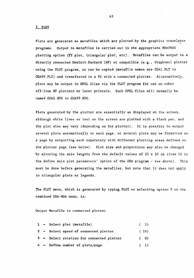
63

7. PLOT

Plots are generated as metafiles which are plotted by the graphics translator .~

programs. Output to metafiles is carried out in the appropriate MDAPROG

plotting option (XY plot, triangular plot, etc). Metafiles can be output to a

directly connected Hewlett-Packard (HP) or compatible (e.g., Graphtec) plotter

using the PLOT program, or can be copied (metafile names are GDAI.PLT to

GDA99.PLT) and transferred to a PC with a connected plotter. Alternatively,

plo.ts may be output to HPGL files via the PLOT program for use on other

off-line HP plotters or laser printers. Such HPGL files will normally be

named GDAI.HPG to GDA99.HPG.

Plots generated by the plotter are essentially as displayed on the screen,

although white lines or text on the screen are plotted with a black pen, and

the plot size may vary (depending on the plotter). It is possible to output

several plots automatically to each page, or several plots may be formatted on

a page by outputting each separately with different plotting areas defined on

the plotter page (see below). Plot size and proportions may also be changed

by altering the axis lengths from the default values of 25 x 20 cm (item 16 in

the define main plot parameters' option of the GDA program - see above). This

must be done before generating the metafiles, but note that it does not apply

to triangular plots or legends.

The PLOT menu, which is generated by typing PLOT or selecting option 5 on the

combined GDA-MDA menu, is:

Output Metafile to connected plotter

1

2

3

4

Select plot (metafile)

Select speed of connected plotter

Select rotation for connected plotter

Define number of plots/page

( 1)

( 10)

( 0)

( 1)

64

5 - Define plotting area within page ( .00 1.00 .00 1.00)

6 Switch output of plots to HPGL on a file

7 - Output selected plot

8 - Output all plots starting at selected one

9 - Delete all metafiles (plots)

10 - Delete all HPGL files

11 - Define metafile path

12 Define HPGL file path

Q Quit

Option [l.12,QJ:

. Options 1-10 of the PLOT menu are dealt with on pages 54-71 of the GDA manual

and are not repeated here. Examples of mineral plots generated under the

MDAPROG and output to Laser printer from HPGL files are given in Figures 1-7.

Two additional options (11 and 12) allow different plot metafile or HPGL file

paths to be specified.

(11) Define metafile path (allows plot metafiles from a different disk drive

or directory to be output to a connected plotter or as HPGL files).

(12) Define HPGL file path (allows plot metafiles to be output as HPGL files

on a different drive or directory).

In either case, the specified path is added to the beginning of the plotfile

name (see examples under GDA, above). Due to line-length limitations of

MS-DOS commands it may not be possible to specify complex pathnarnes for both

metafiles and HPGL files simultaneously. Note that deleting metafiles and

HPGL files (menu items 9 and 10) will only apply to those in the current (i.e.

GDA) directory and only those without prefixes (e.g., GDAl.PLT, but not

ABGDAl. PLT) .

65

8. PRINT A TABLE OF MINERAL ANALYSES (TABMIN)

Tables of mineral analyses, including cation proportions in the structural

formula, can be generated by selecting 17 or the GOA-MDA menu or by directly

calling the program TABMIN. The tables generated have a different format from

that generated by option 17 of the MDA program (print structural formulae

reports). TABMIN output allows reporting of trace elements and arithmetic

derivatives for the analyses, including weight and atomic ratios, such as

2+ Ca/(Ca+Mg+Fe ) etc. The print file generated - TABMIN.PRN - may be

edited/enhanced to camera-ready format using a wordprocessor.

The program is run by entering TABMIN which generates the following menu:

Print oxides GOA file [YIN = metals] (Y):

Geochemical file name [? - LIST] (CURRENT.GOA ): FILENAME

Report/statistics definition file [? - LIST] (OXIOE.MTB ):

Mineral definitions file [? - LIST] (OXIDE.DEF):

Print trace elements [YIN] (N)?

Print Geochemical Data

1 - Generate report on print file TABMIN.PRN

2 - Display report on screen

3 - Oisplay structural formula for single analysis

4 Select major elements

5 - Select trace elements

6 - Select structural formula components

7 - Specify descriptive fields

9 - Select groups to be printed or displayed

10 - Specify range of analyses

11 - Specify group titles

13 - Specify number of analyses per printer page

14 - Specify number of lines on printer page

16 Print values for typed in expressions

18 - Include page header

19 - Change GDA file

Q - Quit

Option [1-19,Q]:

66

These options allow full selection of descriptive fields. analytical data and

derived values (option 16). An example of the output from TABMIN is shown in

Table 8.

67

TABLE 8. EXAMPLE OF OUTPUT FROM TABMIN

DIAMONDIFEROUS XENOLITHS

Sample number N44 Nl4 N40 N27 Analysis number 1 2 3 4 Mineral name OLIVINE OLIVINE OLIVINE OLIVINE Description PI OLIVINE PI OLIVINE PI OLIVINE PI OLIVINE

" Si02 41.42 41.20 41.05 40.87 Cr203 .07 .07 .05 .05 FeD 6.79 7.30 7.57 8.58 MnO .09 .11 .10 .13 NiO .39 .44 .38 .40 MgO 51. 58 51.55 50.85 50.08 CaD .02 .05 .05 .05 Total 100.36 100.72 100.05 100.16

Trace elements In parts per million

Cr 472 465 343 318 Mn 692 815 776 988 Ni 3064 3481 3015 3169 Ca 143 387 346 354

Atomic proportions

Oxygens 4.0 4.0 4.0 4.0 Si .999 .993 .997 .996 Cr .001 .001 .001 .001 Fe2+ .137 .147 .154 .175 Mn .002 .002 .002 .003 Ni .008 .009 .007 .008 Mg 1.854 1. 852 1.840 1. 819 Ca .001 .001 .001 .001 Total 3.001 3.006 3.003 3.003

100Mg/ (Mg+ Fe) 93.12 92.64 92.29 91. 23

68

9. STATS (STATISTICS PROGRAM)

The STATS program generates, on the print file STATS.PRN. various statistical

functions including mean. standard deviation, minimum. maximum. and optional

correlation matrix. A menu. shown below. enables selection of groups,

elements and specification of format. The minerals report definition file

MINREPT.RPT is employed to define output. This can be modified as required to

include other fields. The program STATS is also used to generate a cluster

analysis file for use in the cluster analysis program CLUSTA. details of which

are given in section 10. Options 2-4, and 7-9 also apply in this case. The

program is run by typing STATS or selecting option 6 from the GDA-MDA menu.

The submenu is as follows:

1 Generate statistics report (on file STATS.PRN)

2 Select major elements (all by default)

3 Select trace elements (all by default)

4 Select groups (calculations are based on all selected groups)

5 Specify group titles

6 Specify number of columns per page (1-10, depending on page size)

7 Print values for standard expressions (as for GDA)

8 Print values for typed-in expressions (dataset number and label

must be specified)

9 Drop samples (anomalous samples may be deleted from the

calculations by specifying the appropriate sample number

10 - Generate cluster analysis file (for use in CLUSTER program; a

file name. ????CLU, must be specified)

11 - Change GDA file

Q Quit

A typical printout is given in Table 9.

69

TABLE 9. EXAMPLE OF OUTPUT FROM STATS PROGRAM

GROUPS PROCESSED

PIPE M97 GARNETS PIPE M89 GARNETS

MEANS AND STANDARD DEVIATIONS

Element Mean Standard Minimum Maximum Number of Deviation Items

P205 .02 .01 .02 .05 21 Si02 41.10 .95 38.28 42.29 21 Ti02 .29 .14 .01 .50 21 A1203 18.89 2.46 12.57 22.50 21 Cr203 5.91 3.08 .01 13.31 21 FeO 8.17 4.60 6.71 28.23 21 MnO .35 .13 .24 .89 21 NiO .02 .01 .02 .04 21 MgO 19.64 3.02 7.40 22.12 21 CaO 6.10 1.11 3.72 9.29 21 Na20 .04 .02 .01 .09 21

mg 80.94 11.30 31. 85 84.83 21

CORRELATION MATRIX

P205 Si02 Ti02 A1203 Cr203 FeD P20S 1.00 Si02 -.21 1.00 Ti02 -.24 .42 1.00 A1203 - .41 .38 .13 1. 00 Cr203 .43 -.25 - .12 - .98 1.00 FeO - .15 - .69 - .45 .30 - .43 1. 00 MnO -.17 -.74 -.52 .25 -.36 .95 NiO -.19 - .01 .12 .00 .00 - .06 MgO .02 .88 .55 .02 .11 - .93 CaO .38 - .18 -.15 - .91 .94 - .48 Na20 .03 -.32 .40 - .24 .21 - .08 mg .12 .74 .48 -.24 .38 -1.00

CORRELATION MATRIX

MnO NiO MgO CaO Na20 mg FeO MnO 1.00 NiO - .02 1.00 MgO -.94 .08 1. 00 CaO -.37 .01 .14 1.00 Na20 .01 .28 -.02 .19 1. 00 mg -.96 .06 .96 .42 .07 1.00

' ..

70

10. CLUSTA (CLUSTER ANALYSIS)

Option 7 of the main GDA-MDA menu provides a faci1it~ for cluster analysis.

Cluster analysis is a method of grouping or clustering unknown objects in

which no assumptions are made about the data. There are two basic modes of

classification: Q-mode, in which objects (commonly samples) are classified,

and R-mode, in which attributes (i.e., measurements data such as element

concentrations) made on these objects) are classified.

The method starts with each object as an individual group and joins the most

similar objects and groups together using a particular linkage method until a

single group has been formed. The final grouping is shown by means of a

dendrogram. The similarity between two objects is expressed numerically by a

similarity measure. This program, which is partly based on Bonham-Carter

(1967), gives a choice of two similarity measures, the correlation coefficient

and the proportional similarity coefficient (also known as the cosine-theta

coefficient). There are also two possible linkage methods (in which an object

is linked to a group if it has the highest similarity with the average

similarity measure of the group) available. If the weighted-pair group

average method is used, the new average value for the group is calculated as

the mean of the similarity measure of the new object and the previous group

average. If the unweighted average method is used, the new average similarity

measure of the group is calculated by summing the individual similarity

measures of all objects in the group and dividing by the number of objects in

the group. Unlike the weighted method, this technique does not weight the

group average in favour of the new object. Further details of the cluster

analysis technique are given by Le Maitre (1982).

It is important to note that any dataset for which a major proportion of

samples have zero values should be omitted from the calculations, or the

results may well be biased. In particular, if all selected samples have zero

(i.e., no data) values for any dataset, or if all non-zero values are the

71

same, an error will result when running the program. The offending dataset

should be omitted and the cluster analysis file regenerated (in STATS).

However, note that if all assigned samples have ze;o values, the dataset is

automatically dropped out.

In order to run the cluster analysis program a cluster analysis file must

first be generated in the STATS program, which includes options to add

arithmetic expressions, drop elements and samples, and select groups.

To run the program (which actually includes two parts, CLUSTA and DEND) , type

CLUSTER or option 7 of the GDA-MDA menu to generate the cluster analysis file.

A cluster analysis file (normally of the form ????CLU) must be specified,

followed by the options listed below:

1. Q-mode (default) or R-mode.

2. The similarity measure-correlation coefficient (default) or proportional

similarity coefficient.

3. The linkage method - weighted-pair group method (default) or unweighted.

4. Highest value of similarity (i.e., the upper limit of the Y-axis: 0-1,

1.0 by default).

5. Lowest value of similarity (i.e., the lower limit of the Y-axis: 0-1,

0.0 by default).

Note that the calculations take a significant amount of time to carry out.

Typically, 100 samples for 40 variables will take up to 15 minutes, depending

on the PC. The input data, transformed data matrix, cluster data and

dendrogram details can be printed out from a file CLUSTA.PRN if required.

Example printouts are given in Tables 10 and 11 of Q-mode and R-mode cluster

analysis for a suite of garnets from the Wandagee alkaline intrusives.

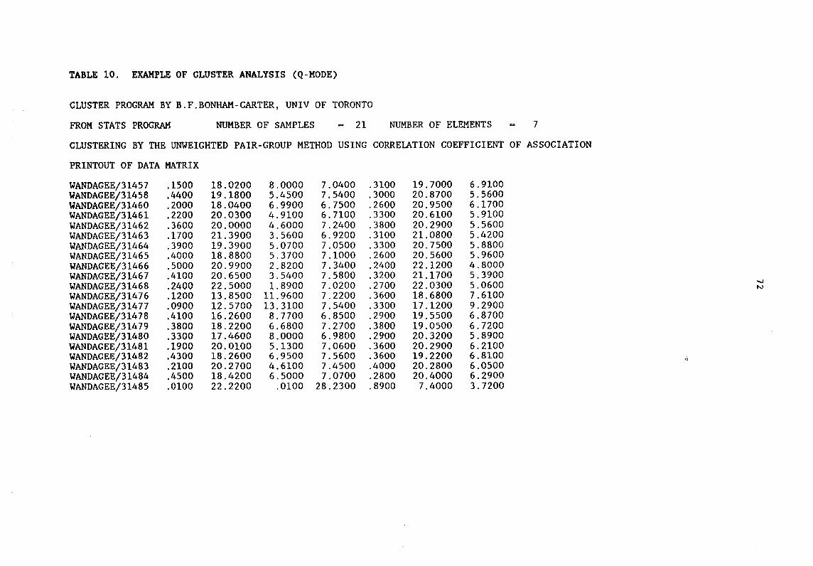
TABLE 10. EXAMPLE OF CLUSTER ANALYSIS (Q-MODE)

CLUSTER PROGRAM BY B.F.BONHAM-CARTER, UNIV OF TORONTO

FROM STATS PROGRAM NUMBER OF SAMPLES = 21 NUMBER OF ELEMENTS 7

CLUSTERING BY THE UNWEIGHTED PAIR-GROUP METHOD USING CORRELATION COEFFICIENT OF ASSOCIATION

PRINTOUT OF DATA MATRIX

WANDAGEE/31457 .1500 18.0200 8.0000 7.0400 .3100 19.7000 6.9100 WANDAGEE/31458 .4400 19.1800 5.4500 7.5400 .3000 20.8700 5.5600 WANDAGEE/31460 .2000 18.0400 6.9900 6.7500 .2600 20.9500 6.1700 WANDAGEE/31461 .2200 20.0300 4.9100 6.7100 .3300 20.6100 5.9100 WANDAGEE/31462 .3600 20.0000 4.6000 7.2400 .3800 20.2900 5.5600 WANDAGEE/31463 .1700 21. 3900 3.5600 6.9200 .3100 21.0800 5.4200 WANDAGEE/31464 .3900 19.3900 5.0700 7.0500 .3300 20.7500 5.8800 WANDAGEE/31465 .4000 18.8800 5.3700 7.1000 .2600 20.5600 5.9600 WANDAGEE/31466 .5000 20.9900 2.8200 7.3400 .2400 22.1200 4.8000 WANDAGEE/31467 .4100 20.6500 3.5400 7.5800 .3200 21.1700 5.3900 WANDAGEE/31468 .2400 22.5000 1. 8900 7.0200 .2700 22.0300 5.0600 -..J

N

WANDAGEE/31476 .1200 13.8500 11. 9600 7.2200 .3600 18.6800 7.6100 WANDAGEE/31477 .0900 12.5700 13.3100 7.5400 .3300 17.1200 9.2900 WANDAGEE/31478 .4100 16.2600 8.7700 6.8500 .2900 19.5500 6.8700 WANDAGEE/31479 .3800 18.2200 6.6800 7.2700 .3800 19.0500 6.7200 WANDAGEE/31480 .3300 17.4600 8.0000 6.9800 .2900 20.3200 5.8900 WANDAGEE/31481 .1900 20.0100 5.1300 7.0600 .3600 20.2900 6.2100 WANDAGEE/31482 .4300 18.2600 6.9500 7.5600 .3600 19.2200 6.8100 ,;

WANDAGEE/31483 .2100 20.2700 4.6100 7.4500 .4000 20.2800 6.0500 WANDAGEE/31484 .4500 18.4200 6.5000 7.0700 .2800 20.4000 6.2900 WANDAGEE/31485 .0100 22.2200 .0100 28.2300 .8900 7.4000 3.7200

TABLE 10 continued

VARIABLES TRANSFORMED TO PERCENT OF THEIR RANGE

PRINTOUT OF TRANSFORMED DATA MATRIX

WANDAGEE/31457 .2857 .5488 .6008 .0153 .1077 .8356 .5727 WANDAGEE/31458 .8776 .6657 .4090 .0386 .0923 .9151 .3303 WANDAGEE/31460 .3878 .5509 .5248 .0019 .0308 .9205 .4399 WANDAGEE/31461 .4286 .7513 .3684 .0000 .1385 .8974 .3932 WANDAGEE/31462 .7143 .7482 .3451 .0246 .2154 .8757 .3303 WANDAGEE/31463 .3265 .8882 .2669 .0098 .1077 .9293 .3052 WANDAGEE/31464 .7755 .6868 .3805 .0158 .1385 .9069 .3878 WANDAGEE/31465 .7959 .6354 .4030 .0181 .0308 .8940 .4022 WANDAGEE/31466 1.0000 .8479 .2113 .0293 .0000 1.0000 .1939 WANDAGEE/31467 .8163 .8137 .2654 .0404 .1231 .9355 .2998 WANDAGEE/31468 .4694 1.0000 .1414 .0144 .0462 .9939 .2406 WANDAGEE/31476 .2245 .1289 .8985 .0237 .1846 .7663 .6984 WANDAGEE/31477 .1633 .0000 1.0000 .0386 .1385 .6603 1.0000 WANDAGEE/31478 .8163 .3716 .6586 .0065 .0769 .8254 .5655 WANDAGEE/31479 .7551 .5690 .5015 .0260 .2154 .7914 .5386 ...., WANDAGEE/31480 .6531 .4924 .6008 .0125 .0769 .8777 .3896 VJ

WANDAGEE/31481 .3673 .7492 .3850 .0163 .1846 .8757 .4470 WANDAGEE/31482 .8571 .5730 .5218 .0395 .1846 .8030 .5548 WANDAGEE/31483 .4082 .7754 .3459 .0344 .2462 .8750 .4183 WANDAGEE/31484 .89&0 .5891 .4880 .0167 .0615 .8832 .4614 WANDAGEE/31485 .0000 .9718 .0000 1.0000 1.0000 .0000 .0000

74

TABLE 10 continued

FROM STATS PROGRAM

CLUSTERING BY THE UNWEIGHTED PAIR-GROUP METHOD

SAMPLE NUMBERS 1 3 2 8 6 11

12 13 15 18 17 19

2 7 17 4

2 20 5 10 2 5

17 6 14 16 14 15

2 9 2 14

17 1 17 2 17 12 17 21

LEVEL OF ASSOCIATION .9934 .9984 .9945 .9879 .9992 .9989 .9983 .9983 .9966 .9971 .9927 .9865 .9918 .9908 .9869 .9799 .9716 .9635 .8613 .6489

ORDER OF SAMPLES FOR DENDROGRAM PLOT

WANDAGEE/31481 WANDAGEEj31483 tJANDAGEE/31461 WANDAGEE/31463 WANDAGEE/31468 WANDAGEE/31457 tJANDAGEE/31460 lJANDAGEE/31458 lJANDAGEE/31465 WANDAGEE/31464 WANDAGEE/31484 WANDAGEE/31462 lJANDAGEE/31467 lJANDAGEE/31466 WANDAGEE/31478 WANDAGEEj31480 lJANDAGEE/31479 lJANDAGEE/31482 lJANDAGEE/31476 WANDAGEE/31477 WANDAGEE/31485

FROM STATS PROGRAM

17 19

4 6

11 1 3 2 8 7

20 5

10 9

14 16 15 18 12 13 21

INFORMATION REGARDING DENDROGRAM PLOT

Y-AXIS PLOTTED BETWEEN 1.0 AND .4

CYCLE NUMBER 1 1 1 1 1 1 2 2 3 3 4 4 4 5 6 7 8 9

10 11

TABLE 11. EXAMPLE OF OUTPUT FROM CLUSTER ANALYSIS (R-MODE)

CLUSTER PROGRAM BY B.F.BONHAM-CARTER, UNIV OF TORONTO

FROM STATS PROGRAM NUMBER OF SAMPLES ... 21 NUMBER OF ELEMENTS = 10

R-MODE ANALYSIS , READ "SAMPLE" AS VARIABLE. CLUSTERING BY THE WEIGHTED PAIR-GROUP METHOD USING PROPORTIONAL SIMILARITY COEFFICIENT

PRINTOUT OF DATA MATRIX

WANDAGEE/31457 .0400 41.5300 .1500 18.0200 8.0000 7.0400 .3100 19.7000 6.9100 .0100 WANDAGEE/31458 .0200 41.8000 .4400 19.1800 5.4500 7.5400 .3000 20.8700 5.5600 .0300 WANDAGEE/31460 .0200 42.0900 .2000 18.0400 6.9900 6.7500 .2600 20.9500 6.1700 .0100 WANDAGEE/31461 .0200 41. 6000 .2200 20.0300 4.9100 6.7100 .3300 20.6100 5.9100 .0100 WANDAGEE/31462 .0200 41. 2400 .3600 20.0000 4.6000 7.2400 .3800 20.2900 5.5600 .0600 WANDAGEE/31463 .0200 41. 9400 .1700 21. 3900 3.5600 6.9200 .3100 21. 0800 5.4200 .0300 WANDAGEE/31464 .0200 41. 5900 .3900 19.3900 5.0700 7.0500 .3300 20.7500 5.8800 .0100 WANDAGEE/31465 .0400 41.1600 .4000 18.8800 5.3700 7.1000 .2600 20.5600 5.9600 .0200 WANDAGEE/31466 .0200 41.9300 .5000 20.9900 2.8200 7.3400 .2400 22.1200 4.8000 .0500 " WANDAGEE/31467 .0200 41. 5500 .4100 20.6500 3.5400 7.5800 .3200 21.1700 5.3900 .0500

Vt

WANDAGEE/31468 .0500 42.2900 .2400 22.5000 1. 8900 7.0200 .2700 22.0300 5.0600 .0300 WANDAGEE/31476 .0400 40.1100 .1200 13.8500 11. 9600 7.2200 .3600 18.6800 7.6100 .0500 WANDAGEE/31477 .0400 39.6100 .0900 12.5700 13.3100 7.5400 .3300 17.1200 9.2900 .0400 WANDAGEE/31478 .0200 40.5800 .4100 16.2600 8.7700 6.8500 .2900 19.5500 6.8700 .0700 WANDAGEE/31479 .0400 40.4800 .3800 18.2200 6.6800 7.2700 .3800 19.0500 6.7200 .0900 WANDAGEE/31480 .0500 40.4400 .3300 17 .4600 8.0000 6.9800 .2900 20.3200 5.8900 .0500 6 .

WANDAGEE/31481 .0200 41. 3100 .1900 20.0100 5.1300 7.0600 .3600 20.2900 6.2100 . 0500 WANDAGEE/31482 .0200 40.7100 .4300 18.2600 6.9500 7.5600 .3600 19.2200 6.8100 .0600 WANDAGEE/31483 .0200 41. 5600 .2100 20.2700 4.6100 7.4500 .4000 20.2800 6.0500 .0400 WANDAGEE/31484 .0200 41.4100 .4500 18.4200 6.5000 7.0700 .2800 20.4000 6.2900 .0500 WANDAGEE/31485 .0200 38.2800 .0100 22.2200 .0100 28.2300 .8900 7.4000 3.7200 .0300

.. i~~

TABLE 11. continued

VARIABLES TRANSFORMED TO PERCENT OF THEIR RANGE

PRINTOUT OF TRANSFORMED DATA MATRIX

WANDAGEE/31457 .6667 .8105 .2857 .5488 .6008 .0153 .1077 .8356 .5727 .0000 WANDAGEE/31458 .0000 .8778 .8776 .6657 .4090 .0386 .0923 .9151 .3303 .2500 WANDAGEE/31460 .0000 .9501 .3878 .5509 .5248 .. .0019 .0308 .9205 .4399 .0000 WANDAGEE/31461 .0000 .8279 .4286 .7513 .3684 .0000 .1385 .8974 .3932 .0000 WANDAGEE/31462 .0000 .7382 .7143 .7482 .3451 .0246 .2154 .8757 .3303 .6250 WANDAGEE/31463 .0000 .9127 .3265 .8882 .2669 .0098 .1077 .9293 .3052 .2500 WANDAGEE/31464 .0000 .8254 .7755 .6868 .3805 .0158 .1385 .9069 .3878 .0000 WANDAGEE/31465 .6667 .7182 .7959 .6354 .4030 .0181 .0308 .8940 .4022 .1250 WANDAGEE/31466 .0000 .9102 1.0000 .8479 .2113 .0293 .0000 1.0000 .1939 .5000 WANDAGEE/31467 .0000 .8155 .8163 .8137 .2654 .0404 .1231 .9355 .2998 .5000 WANDAGEE/31468 1.0000 1.0000 .4694 1.0000 .1414 .0144 .0462 .9939 .2406 .2500 WANDAGEE/31476 .6667 .4564 .2245 .1289 .8985 .0237 .1846 .7663 .6984 .5000 WANDAGEE/31477 .6667 .3317 .1633 .0000 1.0000 .0386 .1385 .6603 1.0000 .3750 WANDAGEE/31478 .0000 .5736 .8163 .3716 .6586 .0065 .0769 .8254 .5655 .7500 .....,

WANDAGEE/31479 .6667 .5486 .7551 .5690 .5015 .0260 .2154 .7914 .5386 1.0000 0-

WANDAGEE/31480 1.0000 .5387 .6531 .4924 .6008 .0125 .0769 .8777 .3896 .5000 WANDAGEE/31481 .0000 .7556 .3673 .7492 .3850 .0163 .1846 .8757 .4470 .5000 WANDAGEE/31482 .0000 .6060 .8571 .5730 .5218 .0395 .1846 .8030 .5548 .6250 WANDAGEE/31483 .0000 .8180 .4082 .7754 .3459 .0344 .2462 .8750 .4183 .3750 WANDAGEE/31484 .0000 .7805 .8980 .5891 .4880 .0167 .0615 .8832 .4614 .5000 WANDAGEE/31485 .0000 .0000 .0000 .9718 .0000 1.0000 1.0000 .0000 .0000 .2500

~

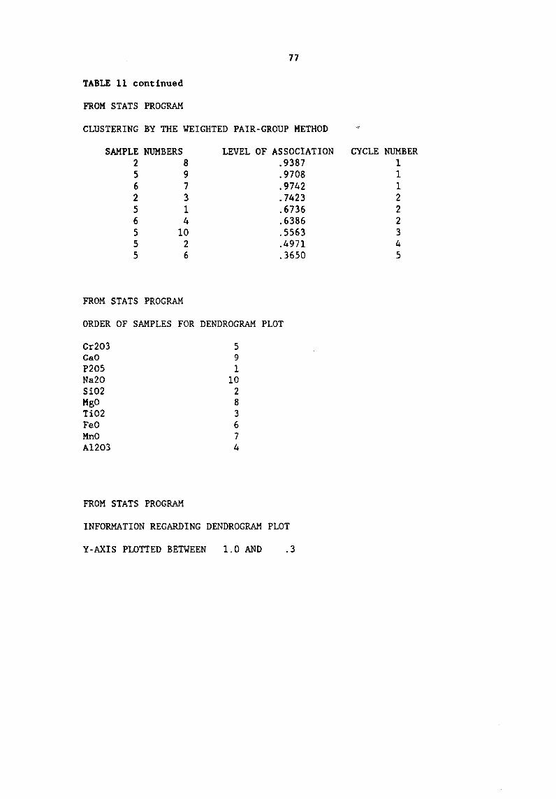
77

TABLE 11 continued

FROM STATS PROGRAM

CLUSTERING BY THE YEIGHTED PAIR-GROUP METHOD

SAMPLE NUMBERS 2 8 5 9 6 7 2 3 5 1 6 4 5 10 5 2 5 6

FROM STATS PROGRAM

LEVEL OF ASSOCIATION .9387 .9708 .9742 .7423 .6736 .6386 .5563 .4971 .3650

ORDER OF SAMPLES FOR DENDROGRAM PLOT

Cr203 5 CaO 9 P20S 1 Na20 10 Si02 2 MgO 8 Ti02 3 FeO 6 MnO 7 A1203 4

FROM STATS PROGRAM

INFORMATION REGARDING DENDROGRAM PLOT

Y-AXIS PLOTTED BETWEEN 1.0 AND .3

CYCLE NUMBER 1 1 1 2 2 2 3 4 5

78

11. DEND (DENDOGRAMS FOR CLUSTER ANALYSIS)

Dendograms of the cluster analysis generated by program CLUSTA may be ~

displayed using program DEND which is invoked by typing DEND or option 8 of

the GDA-MDA menu. The dendograms may be displayed on screen or output to a

metafile (GDAl.PLT to GDA99.PLT). The metafiles may be output to either a

directly-connected HP or HP-compatible plotter or converted to HPGL files for

use on off-line plotters and laser printer using the PLOT program.

Examples of the dendograms generated from the cluster analysis of a suite of

garnets from heavy mineral concentrate from the Wandagee alkaline intrusions

are given in Figs 6A and 6B.

Fig. 6A is an example of Q-mode using the correlation coefficient with no

weightings. The cluster analysis generates similar groupings to that of

Dawson and Stephens (1975) in that groups 5 (magnesian almandine), 10

(low-calcium chrome-pyrope), 12 (knorringitic uvarovite-pyrope) are clearly

separated, and most group 1 (titanium pyrope), group 11 (uvarovite-pyrope) and

group 9 (chrome-pyrope) garnets are clustered. This analysis also recognises

a high correlation between chrome-bearing titanian pyropes and groups 9 and

11.

Fig 6B is an example of R-mode cluster analysis using the proportional

similarity coefficient.

" ..

79

FIG. 6A. Q-MODE DENDOGRAM OF GARNET COMPOSITIONS

CORRELA liON COEFFICIENT OF ASSOCIA liON ·e

tOO .95 .91 .86 .82 .77 .73 .68 .64 .59 .55

I I I I I I I I I I I WAI\[)AGEE/3148'

WANDAGEE/3148~

WAt-VAGEE/3146 ?

WANDAGEE/3146

WANDAGEE/3146

WANDAGEE/3145

WANDAGEE/3146

WANDAGEE/3145

WNVAGt£./3146

WAf'l)AGEE/3146

WAf'l)AGEE/3148

WA~AGEE/3146

WANJAGEE/3146

WAt-VAGt£./3146

WANDAGEE/3147

WAt-eJAGf£./3148

WANDAGEE/3147

WANOAGEE/3148

WANDAGEE/3147

WANDAGEE/3147

WA~AGEE/3148~----------------------------~

FIG. 68. R-MODE DENDOGRAM OF GARNET COMPOSrrlONS

PROPORTIONAL SIMILARITY COEFFICIENT

1.00 .93 .85 .78 .71 .63 .56 .49 .41 .34 .26

Cr203

Co

P20

No2

SiO

Mg

TiO

0

5

0

2

0

2

Fe

Mn

AI20

0 .oz '~

~

I I

CIt o

81

12. UTIL (UTILITIES PROGRAM)

GDA files can be edited with the utilities program (UTIL). Although data held

on a database such as ORACLE may be edited using the database facilities and

data entered through ENTMIN can be edited prior to conversion to GDA files it

is sometimes convenient to use this program to merge files or add average

analyses to a file. There are also facilities for creating new files, editing

existing analyses. adding analyses, changing or adding field names, sorting

samples on a file into numerical or element abundance order, deleting samples

from a file and interrogating files.

The program is run by typing UTIL, or selecting option 1 of the combined

GDA-MDA menu. The UTIL menu is as follows:

1 - Create a new file

(The fields on the the new datafile are aefined by a utilities field

names file, such as OXIDE.UTL; analyses may then be entered using option

5 below)

2 - Interrogate a file

(Descriptive and element fields, a list of sample numbers, and

individual analyses may be displayed)

3 - Define new analysis on screen

(For an existing GDA file; new sample number is specified, and new data

(descriptive or element concentration) added; take care not to specify

an existing sample number).

4 - Modify analysis on screen

(For an existing GDA file; sample number is specified, and new data

(descriptive or element concentration) added)

...

82

5 - Type in new analyses

6 -

(For an existing GDA file; select fields (descriptive or element

concentration) required, then enter data; take care not to specify an

existing sample number)

Type in values for a range of anlyses

(For an existing GDA file; select fields (descriptive or element

concentration) required, specify first and last sample numbers for

samples already on file (in file order), then enter new data for each)

7 - Modify an analysis

(For an e~isting GDA file; give sample number, then new data)

8 = Sort file into analysis order

(i.e., numerical order of sample numbers)

9 - Sort file into element abundance order

(i.e., order of increasing abundance of any selected element)

10 - Merge another file, replacing values

(If the second file has data fields that are not defined in the primary

file, the primary file fields will be expanded to include them. Samples

that are common to both files (same number) will cause values on the

primary file to be replaced by those off the second file. New samples

on the second file are added to the end of the primary file, but their

order may be changed)

11 - Change a field name

(Change an existing field name).

12 - Add a field name.

83

(Descriptive or element concentration in upper or lower case;

concentration data, samples must be re-assigned before any added data

can be plotted; in either c~se, the report definition file (MINREPT.RPT)

will need to be edited).

13 - Write averages to a new file

(Sample numbers must be specified for each average - all samples, and

each assigned group).

14 - Delete a range of analyses.

(First and last sample numbers must be specified, in the order they

appear in the GDA file - not necessarily numerical order).

15 - Write groups to a new file.

(Selected groups can be written from an existing GDA file to a new GDA

file).

16 - Display structural formulae, normalise minerals

The default utilities field names file is UTIL.UTL, which includes all the

standard GDA descriptive fields and elements.

select OXIDE.UTL or METAL.UTL as appropriate.

Minerals applications should

Other files can be set up

(using the same format) if different descriptive and/or numerical fields are

required. The numerical data fields do not necessarily need to contain

element concentrations; any other data for plotting, such as isotopic ratios,

may be entered.

84

13. SUMMARY

1. The first step in using the GOA-MDA system is to get analytical data

(including mineral analyses) in the form of datafiles (GOA files) suitable

for processing. There are several ways of doing this. Mineral analyses

may be entered directly using the ENTMlN program or, alternatively, data

from a database (such as ORACLE) can be entered into the system on ASCII

files. Such files must be transformed into GOA files using the ORACLE

program. Alternatively, data may be entered directly from the keyboard

onto GOA files using the utilities program (DTlL). A new file must be

created, and data are then entered into specified descriptive or element

fields. The UTIL program may also be used to edit or merge existing GDA

files.

2. Before GOA files can be used, samples must be assigned to one or more

groups using the ASSIGN program. This is done by specifying logical

conditions for each group, such as a particular locality, lithology, or

age. Samples in a group are plotted with the same symbol and colour. It

is recommended that the logic is stored on a file for subsequent re-use

and/or editing.

3. Once samples have been assigned to groups, data on GOA files can be used in

the various data-processing programs (MOAPROG, PLOT, TABMIN, STATS,

CLUSTER).

4. The main minerals analysis program (MOAPROG) contains 23 application

programs which enable generation of plots, initially on the PC screen, and

then as plot metafiles for output to plotters, and preparation of tables of

anlayses. Firstly, data (element concentrations, cations calculated from

structural formulae, end-member molecules or any derived arithmetic ratio)

are extracted into datasets. The selected datasets are then used to

produce histograms, XY plots, triangular plots, and box-whisker plots. The

85

required plots are then written to metafi1es for subsequent output to

plotters. Facilities also exist for classification and naming of certain

minerals (pyroxenes, amphiboles, garnets, spinels), and for plotting of

spinel compositions in the reduced or oxidized spinel prism. MOAPROG also

has the facility to generate tables of mineral analyses, structural

formulae and derived arithmetic ratios.

5. Output of plot metafiles to plotters is carried out by the PLOT program.

Plots may either be output directly from metafiles to a connected plotter,

or written to HPGL files for output to an offline plotter or laser printer.

There are facilities for positioning plots on a page, and for outputting a

number of plots on a single page.

6. TABMIN allows printing of tables of mineral analyses including both major

and trace element data, structural formulae, and element ratios or other

derived values. One or more groups may be selected, and the number of

samples per page may be specified.

7. The STATS program is used to calculate statistical functions, comprising

mean, standard deviation, maximum, minimum, and an optional correlation

matrix. It is also used to generate the input file for the CLUSTER

program. One or more groups may be selected for the calculations.

8. CLUSTER is a Q- or R-mode cluster analysis program with dendrogram output.

It requires an input datafile generated in the STATS program.

9. A program OUTGOA can be used to write analyses from GOA to ASCII files for

input to other systems or databases.

86

14. ACKNOW'LEDGEMENTS

The bulk of the programs in the GDA-MDA system were written at BMR. However. '. several of the MDA applications either incorporate specific routines or were

developed from base programs written by others. We particularly thank the

following individuals for generously making available programs/routines for

adaption and incorporation into the system: Nick Ware. Wayne Taylor. Rod

Ryburn. Nick Rock and Ken Currie. We also thank Peter Williams for advice.

87

14. REFERENCES

BONHAM-CARTER, G.F., 1967 - Fortran IV program for Q-mode cluster analysis of .~

non-quantitative data using IBM 7090/7094 computers. Computer Contribution

17, University of Kansas.

CAWTHORN, R.G. & COLLERSON, K.D., 1974 - The recalculation of pyroxene

end-member parameters and the estimation of ferrous and ferric iron content

from electron microprobe analyses. American Mineralogist, 59, 1203-1208.

CURRIE, K.L., 1990 - A simple quantitative calculation of mol fractions of

amphibole end-members. Canadian Mineralogist, (in press).

DAWSON, J.B. & STEPHENS, W.E., 1975 - Statistical analysis of garnets from

kimberlites and associated xenoliths. Journal of Geology, 83, 589-607.

HAWTHORNE, F.C., 1983 - The crystal chemistry of amphiboles. Canadian

Mineralogist, 21, 173-480.

IRVINE, T.N., 1965 - Chromian spinel as a petrogenetic indicator. Part 1.

Theory. Canadian Journal of Earth Sciences, 2, 648-672.

LE MAITRE, R.W., 1982 - Numerical Petrology. Elsevier. Amsterdam.

MITCHELL, R.H. & CLARKE. D.B., 1976 - Oxide and sulphide mineralogy of the

Peuyuk kimberlite, Somerset Island, N.W.T., Canada. Contributions to

Mineralogy and Petrology, 56, 157-172,

RICKWOOD, P.C., 1968 - On recasting of garnet into end-member molecules.

Contributions to Mineralogy and Petrology, 18, 175-198.

88

ROCK, N.M.S, 1987 - A FORTRAN program for tabulating and naming amphibole

analyses according to the International Mineralogical scheme. Mineralogy

and Petrology, 37, 79-88. ~

SOBOLEV, N.V., LAVRENT'YEV. Yu.G., POKHILENKO, N.P., & USOVA, L.V., 1973 -

Chrome-rich garnets from the kimberlites of Yakatia and their paragenesis.

Contributions to Mineralogy and Petrology. 40, 39-52.

SOBOLEV, N.V., POKHILENKO, N.P., LAVRENT'YEV, Yu.G., & USOVA. L.V .• 1975 -

Characeristics of chrome-spinels in diamonds from Yakutian kimberlites.

Doklady Akademii Nauk SSR, 11, 7-24.

WOOD, B.J. & BANNO. 5., 1973 - Garnet-orthopyroxene and orthopyroxene­

clinopyroxene relationships in simple and complex systems. Contributions to

Mineralogy and Petrology. 42. 109-124.

89

APPENDICES

A. SYSTEM LIMITATIONS .,;

There are limits on the capacity of the software due to the limits imposed by

the MS-DOS operating system, HALO graphics package and design decisions.

Max Description

-----------

50 number of groups

11 number of datasets (GDAPROG)

50 number of datasets (SMALLGDA)

4 number of datasets (BIGGDA, MDAPROG)

800 number of assigned samples (GDAPROG)

400 number of assigned samples (MDAPROG)

200 number of assigned samples (SMALLGDA)

2000 number of assigned samples (BIGGDA)

15 number of symbols

8 number of plotter pens

6 number of line types

10 number of logic lines to specify a group

25 number of descriptive fields in GDA file

100 number of element concentrations in GDA file

40 number of element ratios in a spidergram

30 number of elements in a box-whisker plot

100 number of bars in a histogram

20 number of sample numbers typed in for spidergram

5 number of additional points for plots

10 number of columns in report

800 number of samples for least squares line fit (GDAPROG)

200 number of samples for least squares line fit (SMALLGDA)

0 number of samples for least squares line fit (BIGGDA, MDA)

90

15 number of minerals for modelling

10 number of least squares mixing minerals

12 number of olivine addition oxides

5000 number of samples in a GDA file that can be sorted or merged by the DIlL

program

250 number of samples or variables in CLUSTER program

50 number of characters of text for added plot points or text

20 number of additional plot points and/or text lines.

...

91

B. SOFTWARE MAINTENANCE

Most software files are held on directory\GDA\ with the HALO system on \HALO\.

The directory\BIGGDA\ is used for building the larger capacity GOA program

BIGGDA,\SMALLGOA\ is used for the small capacity GDA program SMALLGOA,

and\MINGDA\ for the minerals program MDAPROG .

The programs use software simulation of floating point operations so they will

run on most PCs. The software is written in FORTRAN 77 (Microsoft compiler)

and consists of some 60 programs and over 20 000 lines of source code

occupying approximately 1Mb of disk space. The exception is the arithmetic

calculator routine ARITH.IFT, which is written in a higher level language

IFTRAN. This code must be run through the 1FT preprocessor to produce the

FORTRAN source code. If the system is transported to another computer the

FORTRAN source ARITH.FOR can be used directly, although it is not very

readable. There has not been enough time to convert the routine to standard

FORTRAN.

The insert files for the required directories (GDA, BIGGDA, SMALLGDA, MINGDA)

should be copied into \GOA\.

The whole system can be built by typing 'all' in directory\GDA\. This will

direct the correct files to be copied to the appropriate directory, compiled

and linked.

Each program has a file (with extension .LNK) that is used for linking. Some

programs have a simple overlay structure. All COMMON blocks and major arrays

are on files (with extension .INS) and are inserted by the compiler into the

source code.

92

Changing a system limit requires modifying array definitions in the insert

files, changing the limit definition in GDABLK.FOR and typing 'all' to

rebuild. The separate directories \BlGGDA\and\SMALLGDA\ hold a second set of

definitions for the version 6t the program that allows different numbers of

samples to be handled, and a version of GDABLK.FOR that defines the limits.

Similarly, the \MlNGDA\ directory has insert files for the MDAPROG program.

The least squares line fitting has been dropped from BlGGDA and MDA because of

memory limitations imposed by DOS.

The source code (FORTRAN) files (on each directory) can be backed up to floppy

disks with the command file BACKUP. Only one (1) copy is permitted under

copyright.

The command file CLEANUP.BAT removes surplus files from the GDA directory.

Support for graphics is provided by the HALO package. The system expects to

generate graphics either directly on the sceen or to a metafile. The HALO

package provides translators to output the metacode to HP plotters or to files

of HPGL commands. This code is relatively independent of HALO and if the

module PLTSUB.FOR were rewritten, other graphics packages could be used.

The source code can be installed on an IBM PC as follows:

1. Install Microsoft FORTRAN.

2. Create HALO, GDA, BIGGDA, SMALLGDA and MlNGDA directories.

3. Copy the HALO files for Microsoft FORTRAN to \HALO\.

4. Copy from \HALO\ into \GDA\;

The appropriate plotter translator file(s) which should be renamed,

e.g., copy halo HAL07550.EXE HP7550.EXE,

All *.FNT files (fonts),

93

the appropriate screen graphics driver, which should be renamed as

SCREEN.DEV (e.g., copy halo HALOIBME.OEV SCREEN.OEV),

[If a co-processor is available, the FL commands in ALL. BAT will have

to be edited (to remove /FPi);].

5. Copy the source floppies to \GOA\.

6. Type 'all' under GOA.

The whole system takes over 2 hours to build up, and once built, all HALO and

FORTRAN directory files can be deleted.

94

c. PARAMETER FILES

Various types of parameter file are available for use in entering data or

expressions, defining output, plots etc. New files may be set up as required,

provided the format of the given file type is adhered to.

The GDA manual (pages 133-148) gives examples of the various parameter files

used in extracting data in the GDA program. The main parameter files used for

MDA are:

OXIDE.DEF

METAL.DEF

OXIDE.MTB)

METAL.MTB)

MINREPT.RPT

contains the element to oxide conversion factors for most of

the periodic table. This is used for analyses of silicates

and oxides.

- similar to OXIDE.DEF but used for analyses of metals and

sulphides.

- report definition files used in MDAPROG.

Report definition file containing some 23 common major

elements as oxides to be used in generating reports of

analyses of oxides using TABMIN.

To avoid confusion and to enable a listing when the? - prompt appears, it is

recommended that any new files are named according to the nomenclature above

(see also pages 133-134 of the GDA Manual). OXIDE.DEF, OXIDE.MTB and

MINREPT.RPT are given in the following pages.

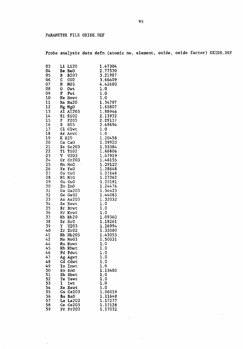
95

PARAMETER FILE OXIDE.DEF

Probe analysis data defn (atomic no, element, oxide, oxide factor) OXIDE.DEF

03 04 05 06 07 08 09 10 11 12 13 14 15 16 17 18 19 20 21 22 23 24 25 26 27 28 29 30 31 32 33 34 35 36 37 38 39 40 41 42 44 45 46 47 48 49 50 51 52 53 54 55 56 57 58 59

Li Li20 Be BeO B B203 C C02 N N03 o Owt F Fwt Ne Newt Na Na20 Mg MgO Al Al203 S1 S102 P P205 S S03 C1 C1wt Ar Arwt K K20 Ca CaO Sc Sc203 Ti Ti02 V V203 Cr Cr203 Mn MnO Fe FeO Co CoO Ni NiO Cu CuO Zn ZnO Ga Ga203 Ge Ge02 As As203 Se Sewt Br Brwt Kr Krwt Rb Rb20 Sr SrO Y Y203 Zr Zr02 Nb Nb205 Mo Mo03 Ru Ruwt Rh Rhwt Pd Pdwt Ag Agwt Cd Cdwt In Inwt Sn SnO Sb Sbwt Te Tewt I Iwt Xe Xewt Cs Cs203 Ba BaO La La203 Ce Ce203 Pr Pr203

1.47304 2.77530 3.21987 3.66409 4.42680 1.0 1.0 1.0 1. 34797 1.65807 1.88946 2.13932 2.29l37 2.49694 1.0 1.0 1.20458 1.39920 1. 53384 1.66806 1.47919 1.46155 1.29122 1.28648 1. 27148 1.27262 1. 25181 1.24476 1.34423 1.44083 1.32032 1.0 1.0 1.0 1.09360 1.18261 1. 26994 1.35080 1.43053 1. 50031 1.0 1.0 1.0 1.0 1.0 1.0 1.13480 1.0 1.0 1.0 1.0 1.06019 1.11648 1.17277 1.17128 1.17032

60 Nd Nd203 1.16639 62 Sm Sm203 1.15962 63 Eu Eu203 1.15793 64 Gd Gd203 1.15262 65 Tb Tb203 1.15101 66 Dy Dy203 1.14770 67 Ho Ho203 1.14551 68 Er Er203 1.14349 69 Tm Tm203 1.14206 70 Yb Yb203 1.13869 71 Lu Lu203 1.13716 72 Hf Hf203 1.17929 73 Ta Ta205 1. 22105 74 W W02 1.17405 75 Re Rewt 1.0 76 Os Oswt 1.0 77 lr lrwt 1.0 78 Pt Ptwt 1.0 79 Au Auwt 1.0 80 Hg Hgwt 1.0 81 Tl Tlwt 1.0 82 Ph PbO 1.07723 83 Bi Biwt 1.0 90 Th Th02 1.13790 92 U U308 1. 17925

PARAMETER FILE MINERAL.MTB

Report definiton file MINERAL.MTB Major elements 62 U308 Mo03 P205 Nb20S Ta205 Si02 To02 Ge02 Zr02 W02 Th02 B203 A1203 Sc203 V203 Cr203 Ga203 As203 Y203 Cs203 La203 Ce203 Pr203 Nd203 Sm203 Eu203 Gd203 Tb203 Dy203 Ho203 Er203

96

Tm203 Yb203 Lu203 Hf203 Fe203 FeO MnO NiO MgO CoO CuO ZnO CaO SrO BaO PhO Li20 Na20 K20 Rh20 o F Ne Cl Ar Br Kr I Xe C02 N03 Trace elements 62 U Mo P Nb Ta Si Ti Ge Zr lJ Th B Al Sc V Cr Ga As y Cs La Ce Pr Nd Sm Eu Gd Th Dy H

97

Er Tm Yb Lu Hf Fe Fe3+ Fe2 Mn Ni Mg C Cu Zn Ca Sr Ba Pb Li Na K Rb F Ne Cl Ar Br Kr I Xe C N Description 7

fields

SAMPNO ANALNO MINERAL MINDERSCR STRATGROUP STRATUNIT STRATHT

Sample number Analysis number Mineral name Description Stratigraphic Group Stratigraphic unit Stratigraphic height

PARAMETER FILE MINREPT.RPT

Report definition file MINREPT.RPT Major Elements 23 P20S P20S NB20S Nb20S ZR02 Zr02 5102 Si02 TI02 Ti02 AL203 AL203 CR203 Cr203 V203 V203 Y203 Y203 FE203 Fe203 FEO FeO MNO MnO NIO NiO CUO CuO ZNO ZnO

98

MGO CAO SRO BAO NA20 K20 F

MgO CaO SrO BaO Na20 K20 F Cl CL

Trace o

elements

Description fields 6 ANALNO SAMPNO MINERAL MINDESCR OXYGENS CATIONS

Analysis number Sample number Mineral Mineral description Number of Oxygen atoms Number of cations

99

100

D. GRAPHICS OVERLAY FILES

Graphics overlay files are used to add extra information, such as text and

field boundaries, to XY and triangular plots. In particular, field boundaries

used in various mineral comparisons can easily be superimposed on the

appropriate plot.

The format of a typical .GRF file is as follows:

Graphics overlay file - TSTGDA.GRF

* * example file

* * Font 11

Pen 4

Textsize

0.5

Text

Aa Bb Cc 1234567890

68.0 0.9

* Pen 5

Linetype 4

Line 3

68.0 0.2

70.0 0.5

74.0 0.8

Pen 2

Line type 2

Line 2

68.0 0.2

101

99.0 0.4

* Linetype 1

Pen 3

Symbo1size

2.0

Symbol 6

70.0 0.5

The first line, which specifies the file type, is mandatory, and any lines

beginning with a * are used for explanatory comments. Text can be displayed

by specifying font, pen colour, and textsize, followed by the text itself and

the XY co-ordinates of the beginning of the text. Symbols require pen colour,

symbol size and symbol number, followed by the XY co-ordinates. Lines require

pen colour, linetype number, and the number of co-ordinate pairs (X, Y) needed

to define the line, followed by the same number of co-ordinates. For straight

lines, only the beginning and end co-ordinates, and, if appropriate, the

co-ordinates of each intermediate change of orientation (kink) need be given.

For example, a V-shaped line would require three co-ordinate pairs. Curved

lines require a relatively large number of closely spaced co-ordinates. Any

number of intersecting or parallel lines may be specified. Note that it is

only necessary to re-define the font, symbol, 1inetype, pen, text size, and

symbol size if these need to be changed. Font, pen, symbol, and linetype

numbers are given in the 11-15 character field on the same line, whereas

decimal values (symbol size and text size) must be on the following line.

Each XY co-ordinate is separated by a comma. Only the X (left) and Y (upper)

co-ordinates should be given for triangular plots. If the axes limits

selected for XY plots are less than those covered by the overlay file, lines

will be truncated on the screen, but not necessarily on the paper plots due to

limitations of HALO.

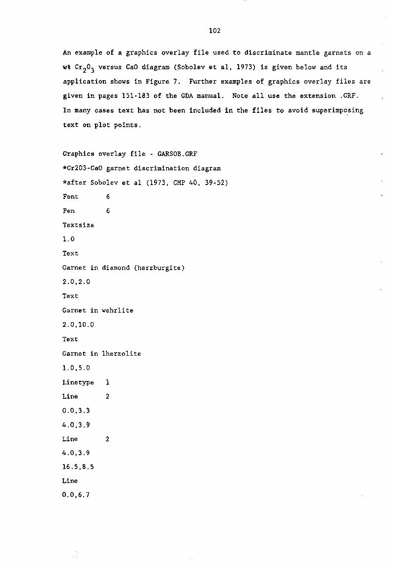
102

An example of a graphics overlay file used to discriminate mantle garnets on a

w% Cr203 versus CaO diagram (Sobolev et al, 1973) is given below and its

application shows in Figure 7. Further examples of graphics overlay files are

given in pages 151-183 of the GDA manual. Note all use the extension .GRF.

In many cases text has not been included in the files to avoid superimpo.sing

text on plot points.

Graphics overlay file - GARSOB.GRF

*Cr203-CaO garnet discrimination diagram

*after Sobolev et al (1973, CMP 40, 39-52)

Font 6

Pen 6

Textsize

1.0

Text

Garnet in diamond (harzburgite)

2.0,2.0

Text

Garnet in wehrlite

2.0,10.0

Text

Garnet in lherzolite

1.0,5.0

Line type 1

Line 2

0.0,3.3

4.0,3.9

Line 2

4.0,3.9

16.5,8.5

Line

0.0,6.7

6.0,6.1

Line 2

6.0,6.1

16.5,10.0

103

FIG. 7. x:f PLOT OF GARNETS WITH GRAPHICS OVERLAY FLE

16 • Pipe M89 garnets

14 A Pipe M97 garnets

12 ~ Garnet • wehrlite 10 In +' ~

8 t-

O 0 ~

c ()

6 • • 4

Garnet • diamond (harzburgite) 2 In

2 4 6 8 10 12 14 16 Cr203 wt "

..

105

E. TRANSFER OF DATA FROM ANU/BMR ELECTRON PROBE MICROANALYSER

Data are transferred from the ANU/BMR Cameca (Camebax) EPMA to ASCII files on

an IBM PC floppy disk using the program PROCOMM. The data can then be read

into the GDA/MDA system using program PROBE. To transfer analyses from the

Dec PDP 11 controlling the Cameca to the IBM PC at the probe the following

instructions apply.

1. Turn on PC (PC should be in the MCA directory);

2. Type CD\PROCOHM followed by GO when in PROCOMM directory

(This will instal the PROCOMM program used to transfer the data);

3. Insert floppy disk into Drive B;

4. Press FlO (for help Menu);

5. Selection 'ASCII Receive' option by pressing F6;

6. Enter file name specifying the B drive i.e. B:filename;

7. On PDP 11 exit to operating system;

8. Type R PCFILE (return);

9. Respond to 'Enter header line' request by entering header;

10. Respond to 'Enter lower analysis number (1 to 1000 for current file)'

by entering the lowermost analysis number;

11. Respond to 'Enter upper analysis number (1 to 1000 for current file)'

by entering the uppermost analysis number;

12. Respond to 'Analyses for deletion (1 to 1000 current file)' by

entering up to 20 analyses to be deleted. Enter 0 for no deletions;

13. Repeat for subsequent groups and enter 0 for lower analysis number to

end;

This process generates file IBMPC.TXT (IBMPC.TXT; 1, 2, etc, for

several files);

14. Type COPY IBMPC.TXT.TT3: [Note: Do not hit return key until PROCOMM is

ready to receive the file - see 1-6];

15. Hit RETURN/ENTER key on PDP 11 keyboard to commence transfer;

16. On completion of transfer of data, press ESC to exit;

17. Exit from PROMM (ALT X COMMAND);

..

106

18. Check floppy disk for correct transfer of data.

The data is entered into the MDA/GDA system via program PROBE. Program PROBE

requires the name of the data file and the new Oracle (.ORC) file. The

program then scans the data file for the listed elements and reports any

errors/corrupted data. Descriptive information - sample number (SAMPNO),

mineral (MINERAL), mineral description (MINDESC), the number of oxygens

(OXYGENS), and, if required, the number of cations in the ideal formula

(CATIONS) to enable calculation of Fe203 and FeO based on stoichiometry -

are then entered. Incorrect entries can be corrected interactively and poor

analyses can be rejected from the Oracle file. The program stops when it

reacheas the end of file character 99 in the element listing.

NOTE: If it is necessary to exit from PROBE and resume later a new .ORC file

must be nominated to avoid overwriting the original file used in the previous

session, i.e., program PROBE does not allow appending of files.