mineral data analysis system (mda): reference … j j j j j bmr geology and geophysics australia...

J J J J J J

BMR GEOLOGY AND GEOPHYSICS AUSTRALIA

I

MINERAL DATA ANALYSIS SYSTEM (MDA)

REFERENCE MANUAL

Record 1992/3

BMR PUi;Lh.":h.~ -(LENDING S):.,L.l.1....,."

. .. + .. ~. ~.

by AL Jaques, L Simons and JW Sheraton Bureau of Mineral Resources, Geology and Geophysics

BM RGEOLOGY ANDGEOPHYSICSAUSTRALIA

MINERAL DATAANALYSIS SYSTEM (MDA)

REFERENCE MANUALRecord 1992/3

by AL Jaques, L Simons and JW Sheraton

MINERALS AND LAND USE PROGRAM

* R 9 2 0 0 3 0 1 *

DEPARTMENT OF PRIMARY INDUSTRIES AND ENERGY

Minister: The Hon. Alan Griffiths

Secretary: G. L. Miller

BUREAU OF MINERAL RESOURCES, GEOLOGY AND GEOPHYSICS

Executive Director: R.W.R. Rutland AO

Commonwealth of Australia, 1992

ISSN 0811 062X

ISBN 0 642 17057 6

This work is copyright. Apart from any fair dealing for the purposes of study, research,criticism or review, as permitted under the Copyright Act, no part may be reproduced byany process without written permission. Inquiries should be directed to the PrincipalInformation Officer, Bureau of Mineral Resources, Geology and Geophysics, GPO Box378, Canberra, ACT 2601.

2

NOTICE

While every effort has been made to ensure that the software is as error-free as possible,BlVIR cannot undertake to provide any formal software support to purchasers of the systemif problems do arise. Nevertheless, we will attempt to assist users who encounterdifficulties, and would appreciate being informed of any bugs which may becomeapparent. Please refer enquiries about the software to

Dr John Sheraton or Dr Doone WybornMinerals and Land Use ProgramBureau of Mineral ResourcesGPO Box 378CANBERRA ACT 2601(phone: (06) 2499111 fax: (06) 2576465)

Enquiries regarding purchase of the system should be made to the BMR Sales Centre atthe same address (phone (06) 2499519, fax (06) 2576466).

3

ABSTRACT

MDA (Mineral Data Analysis) is a comprehensive IBM PC-based system for processing mineral chemical data, particularly those obtained by electron probe microanalyser. It is designed to use mineral chemical data which may be entered into files from the keyboard, transferred from files generated on the microprobe, or retrieved from a database such as ORACLE. MDA is an extension of GDA (Geochemical Data Analysis), BMR's comprehensive PC-based system for processing whole-rock geochemical data. The programs are written in FORTRAN 77 (Microsoft compiler) and use the MicroGlyph Systems Sciplot graphics package for plotting. The system includes facilities for generating plots (histograms, XY plots, triangular plots, etc), calculating statistical functions (e.g., mean, standard deviation, regression lines, correlation coefficients and cluster analysis) as well as enabling calculation of end-member molecules, the classification and naming of minerals, and the printing of tables of analyses. Plots can be displayed on screen for inspection and editing before being output to a plotter or other device. Other programs allow samples to be assigned to groups for plotting purposes, and editing and merging of data files.

MDA is currently used at BMR to process all mineral chemical data obtained by electron probe micro-analyser for petrology-oriented research projects. The package could be readily employed in anyproject requiring manipulation of mineral analyses. It is likely to find particular application in the field of diamond exploration which relies heavily on the chemical discrimination of indicator minerals.

5

CONTENTS

1 INTRODUCTION . . . . . . . . . . . . . . . . · . 10

10

12

12

12

13

13

13

1.1 Command Summary

1.2 Parameter Files

1.3 Printouts

1.4 User Interface

1.5 Software

1.6 Hardware Requirements

1.7 GDA File

2 INSTALLATION . . . . . 3 DATA ENTRY . . . . . . . . .

3.1 From microprobe (PROBE)

3.2 From keyboard (ENTMIN)

3.3 From Oracle database

3.4 Using UTIL program

4 ORACLE ...... .. .

. . . . .

5 ASSIGN ........ . . . . . . . . . . . 6 MINERAL DATA ANALYSIS (BMRMDA)

6.1 Extract values for typed-in expressions

6.2 Extract structural formulae into datasets

6.3 Extract pyroxenes into datasets

6.4 Extract amphiboles into datasets

6.5 Extract spinels into datasets

6.6 Extract garnets into datasets

6.7 Select groups for display

6.8 Delete all plot files

6.9 Define new plot parameters

6.10 Display data sets .

6.11 Display histograms . .

6.12 Display XY plot . . .

6.13 Display triangular plot

6.14 Display legend

6.15 Display spinel prism

6.16 Display box-whisker plot

6.17 Print structural formulae report

6.18 Print pyroxenes report

6

· . 14

. . . . 15

15

15

18

18

. 19

· . 24

. . . 27

29

31

32

33

34

34

35

35

35

37

38 41

44

46

46

49

51

52

6.19 Print amphiboles report .....

6.20 Print amphibole classification report

6.21 Print spinels report . . . . . .

6.22 Print garnet report ..... .

· 54

· 56

· 58

· 60

7 VECTOR ........... . . . . . . . . . . . . · 62

7.1 Vector Program ....... ............ 62

8 PRINT A TABLE OF MINERAL ANALYSIS (TABMIN) . . . . 67

9 STATS (STATISTICS PROGRAM)

10 CLUST A (CLUSTER ANALYSIS) . . . . . . . . 70

· 72

11 BMRDEND (DENDOGRAMS FOR CLUSTER ANALYSIS) .. 79

12 UTIL (UTILITIES PROGRAM)

13 SUMMARY ..... .

14 ACKNOWLEDGEMENTS

REFERENCES

APPENDICES

A - SYSTEM LIMITATIONS

B - PARAMETER FILES . . . .

C - GRAPHICS OVERLAY FILES

. . . . . . . . .

7

· 82

. . • . 84

. . . . . 86

. . . . . 87

. . . . 88

· 88

· 89

· 97

LIST OF TABLES

1. Example of statistics output from XY plot 42

2. Example of structural formulae-report 51

3. Example of pyroxene report 53

4. Example of amphibole report 55

5. Example of amphibole classification report 56

6. Example of spinel report 59

7. Example of garnet report 61

8. Example of output from TABMIN 69

9. Example of output for ST ATS program 71

10. Example of output from CLUSTA program (Q-mode) 73

11. Example of output from CLUSTA program (R-mode) 76

8

LIST OF FIGURES

1. Example of stacked histogram plot of garnet compositions in terms of wt% of Cr203, MgO, and CaO. ..................... 40

2. Example of XY plot showing compositional variation amongst diamond facies chromites in terms of 100 Mg/(Mg+Fe2+) and 100 Cr/(Cr+Al). . . . . . . 43

3. Example of XYZ plot of garnets from two of the Wandagee alkaline ultrabasic

pipes in terms of wt% CaO, MgO and Cr203. . . . . . . . . . . .. 45

4a. Example of oxidized spinel prism plot showing compositional variation of groundmass spinels in the West Kimberley lamproites. ....... . 47

4b. Example of reduced spinel prism plot for groundmass spinels in the West Kimberley lamproites. .................... 48

5. Example of box-whisker plot showing compositional variation of chromites in diamond. . .......................... 50

6a. Example of Q-mode dendogram for garnets from two of the Wandagee alkaline ultrabasic intrusions. Cluster analysis using correlation coefficient of association and no weighting. . . . . . . . . . . . . . . . . . . . . . . . . 80

6b. Example of R-mode dendogram for same garnets as in Figure 6A. Cluster analysis using proportional similarity coefficient. . . . . . . . . . . . . . . . 81

7. Example of XY plot with graphics overlay file. Plot shows compositional variation in garnets from two of the Wandagee alkaline ultrabasic intrusions in terms of wt%

Cr203 versus CaO compared to the fields for garnet in mantle harzburgite, lherzolite and wehrlite as defined by Sobolev et al. (1973). The overlay data are contained in file GARSOB.GRF. . . . . . . . . . . . . . . . . . . 99

8. Clinopyroxene classification of Poldervaart & Hess (1951), produced using graphics overlay file PYROXENE.GRF. . . . . . . . . . . . . . . 101

9

1 INTRODUCTION

The mineral data analysis (MDA) system is an extension of the Bureau of Mineral Resources Geology and Geophysics (BMR) IBM PC-based geochemical data analysis (GDA) system to enable processing of mineral analyses obtained by electron probe microanalyser. It was developed by Lloyd Simons, a contract programmer with Liveware Computer Services, for BMR. The MDA system utilises many of the GDA programs which enable transfer of data from an Oracle database, processing, the generation of plots (histograms, XY plots, triangular plots, and box-whisker plots) and the calculation of statistical functions, but includes a number of programs which are specific to mineral chemical analyses. These programs permit entry of mineral analyses into files, the calculation of structural formulae, estimation of Fe203 and Fe3+ content, calculation of end-member components, classification and naming of certain minerals, and specialised plots such as the spinel prism.

This manual is intended to explain the general operation of the system which is largely menu-driven. It should be read in conjunction with the GDA manual (BMR Record 199211) but the MDA system can be operated without prior experience or knowledge of GDA. For both systems a basic knowledge of IBM-compatible PCs and MS-DOS is assumed. A summary outlining the operation of the system is given in Section 13.

1.1 COMMAND SUMMARY The MDA system comprises three main programs - ENTMIN, BMRMDA and TAB MIN. MDA also uses eight other programs which are common to GDA and MDA. These are linked with the GDA programs for handling geochemical analyses into a common GDA-MDA starting menu shown below. The common menu is called by keying MDA (or GDA). Each of the programs can then be run by typing the appropriate number from the menu or the name of the program.

ASSIGN - assigns the samples to groups according to logical operations on the descriptive fields. Each group is processed and represented on screen as an entity, e.g., all samples in a group are displayed with the same symbol and colour.

CLUSTER - Q- and R-mode cluster analysis with dendrogram output (comprises two programs - CLUSTA and BMRDEND).

BMRDEND - generates the dendrogram output from the cluster analysis program (CLUSTA).

ENTMIN - accepts mineral data entered from the keyboard and writes them out in Oracle format.

BMRMDA - the core program of MDA. This enables data to be extracted into datasets, either direct!1t or using specified arithmetic expressions or standard operations (e.g., Mg/(Mg+Fe +)); calculation of end-member components; classification and naming of minerals; plots of these datasets can be previewed on the PC screen and output to files for later plotting.

ORACLE - reads the ASCII file which is either created by keyboard entry or imported from a database (e.g., Oracle) and writes the data to an internal (GDA) file for subsequent processing.

10

~~-------- --- ----<-

1 INTRODUcrION

OUTGDA - writes contents of a GDA file to an ASCII file for entry to a data base (e.g., ORACLE) or for export and/or processing by other systems.

VECTOR - outputs graphics files (from MDA and GDA) to a plotter or other device.

STATS - generates correlation matrices and sample statistics.

TABMIN - generates tables of analyses including major and trace elements, structural formulae, and cation ratios as required.

UTIL - utilities that allow editing of GDA files.

Users of the earlier versions of GDA and MDA, which utilised HALO graphics, should note that BMRGDA, BMRPMOD, BMRDEND and BMRMDA replace GDAPROG, PETMOD, DEND and MDAPROG respectively. However, both versions can be run on the same PC if required.

The GDA-MDA System is linked by a common menu run by the command MDA (or GDA) as follows:

GEOCHEMICAL AND MINERAL DATA ANALYSIS *** COMMON PROGRAMS (GDA and MDA) ***

1 = Utility functions (UTIL)

2 = Convert from Oracle format (ASCll) file to GDA file (ORACLE)

3 = Assign samples to groups (ASSIGN)

4 = Output to plotter / printer (VECTOR)

5 = Statistical functions (STATS)

6 = Cluster analysis (CLUSTA)

7 = Dendrograms for cluster analysis (BMRDEND)

8 = Export GDA file as ASCII file (OUTGDA)

*** GEOCHEMICAL - GDA ONLY *** 9 = Geochemical data analysis (BMRGDA)

10 = Generate tables of analyses (TABLE)

11 = Petrological modelling (BMRPMOD)

*** MINERALS - MDA ONLY *** 12 = Enter mineral data from keyboard (ENTMIN)

13 = Minerals data analysis (BMRMDA)

14 = Generate tables of anlyses (TABMIN)

The TABLE program can be used for mineral data, but does not allow printing of structural formulae (see GDA manaual for further details)

11

1 INTRODUCfION

1.2 PARAMETER FILES System parameters, such as element to oxide conversion factors, are held on files which can be modified with a text editor or word processor (e.g., WORD STAR non-document mode). Some files are generated during processing and can also be modified. Care must be taken to preserve the format (logical struc ture) of the fIles. The first line of a file must not be changed as it is used to specify the type of fIle.

1.3 PRINTOUTS Printout is generated on files that can be printed or input to a word processor. The file is generally the name of the program with extension .PRN (e.g., STATS.PRN, TABMIN.PRN), but MDA.PRN is the output file for BMRMDA. Such files can be edited in any way required, as they are not used by the MDA system.

1.4 USER INTERFACE The programs are controlled by selection of options from menus at the system and program level and by typing answers to questions. The standard DOS command interface is used, i.e., no command is processed until the Enter key is pressed, and the backspace key can be used to correct typing errors.

Program menus are of the following form:

1 = Histogram

2 =XYplot

3 = Triangular plot

Q = Quit

Option (1-3, Q) (exit)

where the option is chosen by typing the related number (followed by Enter). In some cases a hierarchy of menus is presented; the Enter keystroke will cause control to return to the previous menu (until the first is reached).

Questions and commands are of the following fonn, e.g.,

Type marker [0.1-2.0cm] (0.5):

Do you want to display sample names [YIN] (Y)?

Arithmetic expression [?=help]:

where general infonnation, range of values, etc., are given in [ ] and any default values that will be taken on the Enter keystroke are given in ( ).

Each answer is checked by the system, and,if invalid, a message may appear and the question is repeated.

Values must be given within any indicated range, and a decimal point should be included if (and only if) the indicated range of default values shows it.

Any program can be tenninated (aborted) by using the CONTROL and C keys to return to the operating system.

12

1 INTRODUCTION

1.5 SOFTWARE All the software is written in Microsoft FORTRAN 77 (version 4.1). Microglyph Systems Sciplot is used for graphics to provide support for HP plotters, dot matrix printers, laser printers and several displays (EGA, Hercules, CGA and VGA).

1.6 HARDWARE REQUIREMENTS An mM PC or compatible is required with 640K RAM, a 10 megabyte hard disk (the actual GDA and MDA programs require about 6 MB, and a Hercules, EGA, CGA or VGA colour graphics card. An HP compatible plotter is required for hardcopy graphics and a printer for reports (or monochrome graphics).

1.7 GDAFILE Like the GDA system, MDA operates on sets of assigned samples held in geochemical (GDA) files. Each sample is one random access record in the file, and is identified by its sample number.

The data for each sample are in two parts. The first part consists of descriptive data, of which only the sample number is mandatory. Other descriptive fields used in the standard definition files OXIDE.DEF and MET AL.DEF include the analysis number, the mineral name, and number of cations and oxygens in the mineral formula. Descriptions can be up to 32 characters. The descriptive fields are used to assign samples to groups for display. The other part consists of concentrations for a defined set of elements. Major elements (as oxides for silicate and oxide minerals or elements for metals and sulphides) are given in weight percent, whereas trace elements are given in parts per million (PPM). Zero is held if there is no value for an element. Where an element was not detected, a value of the negative of the detection limit is stored (a value of half the detection limit is used in most processing).

The names of the descriptive and element fields are up to 10 characters long and can include any information desired, but the sample number must have the name' SAMPNO'; the analysis number (ANALNO) is optional, but will commonly be required, since there may well be a number of analyses from the same sample.

The data can be extracted from an existing database, transferred from EPMA in the form of an ASCII file or entered from keyboard using the program ENTMIN. All data must be in external Oracle database format before they can be made into a GDA file using the ORACLE program.

Alternatively, data can be typed directly into aGDA file with the utilities program (UTIL), which can also be used to edit GDA files. GDA fIles should be given names with the extension .GDA. It is recommended that the same Oracle file name be used with the GDA extension (e.g., BOWHILL.ORC and BOWHILL.GDA).

NOTE: The facility to list all Oracle-format and GDA fIles (by typing '?') when running programs requires the correct fIle extension.

Before data in a GDA fIle can be processed, samples must be assigned to groups using the ASSIGN program. After assignment of samples the various data-processing programs (BMRMDA, VECTOR, TABMIN, STATS, CLUSTER, etc.) can be used.

13

2 INSTALLATION

The MDA system requires the GDA system for its operation since many programs are common (however, GDA may be run without MDA). The software is provided on floppy disks in either 5.25" or 3.5" format, and is installed on the PC as follows:

• Set up a directory (normally \GDA\) on the hard disk by typing mkdir GDA;

• Copy the contents of all the floppy disks to this GDA directory; (if GDA is already on the hard disk, copy only the additional MDA programs and files);

• Edit the file SITE.DEF to specify the appropriate graphics card for your system (EGA or VGA). The HP plotter needs to be specified only for the versions of GDA and MDA which use the HALO graphics package. A sample file is:

Site Definition File SITE.DEF

8 Number of pens, the (red,green,blue) values & names follow 1 1.001.00 1.00 Black White on screen 2 1.00 0.00 0.00 Red 3 0.00 1.00 0.00 Green 4 0.00 0.00 1.00 Blue 5 1.00 1.00 0.00 Yellow

6 1.00 0.00 1.00 Magenta 7 1.00 0.50 0.00 Brown 8 1.00 0.50 0.50 Light Red HP7550 The HP plotter model

a The communications port, O=portl, 1=port2 a Autofeed, 1=7550 autofeed, O=none

10 Speed in cm/second 40.4 Plotter page width in cm A3 page, assumed in SW 28.5 II II height

10760 Offline plotter page width in HPGL address units - 400*size

07600 "" II height II II " EGA Graphics card 0.00 0.00 0.00 Screen background colour The table of pens and their colours should be set up to agree with the actual plotter pens so plots previewed on a colour screen will agree (or the pens could be installed in the plotter in the correct order). Colours are given as (red,green, blue) triples. The plotter page size must be correct if actual sizes are to be used when specifying plot parameters. The software is set up with defaults for A3 paper. For other output devices, the page size is set by the user when the BMRMDA program is run.

Three files in Oracle format, GARNET.ORC and AMPHIB.ORC (for oxide and silicate minerals) and SULPHIDE.ORC (for metals and sulphide minerals), are provided for use when trying out the system.

14

3 DATAENTRY

Data may be entered into the MDA system by direct transfer from the EPMA via an ASCII file, from keyboard using the ENTMIN program, or by extraction from a database such as the BMR Oracle database.

3.1 FROM MICROPROBE (PROBE)

Data may be transferred directly from the electron probe microanalyser to the GDA/MDA system in the form of an ASCII file. Such a file must have a particular format, as described under ORACLE (see below).

3.2 FROM KEYBOARD (ENTMIN)

This program enables data to be entered from keyboard and is run by typing ENTMIN or nominating the appropriate option number (15) on the menu.

• The program first requires the name of the Oracle format file (e.g., BOWHILL.ORC). [Existing files with the extension .ORC may be listed by typing '?'].

• The mineral definition file must then be entered. OXIDE.DEF (the default option) is used for silicates and oxides, and MET AL.DEF for metals and sulphides.

• The type of data to be entered - either oxides (as in silicates and oxide minerals) or elements (as in sulphides and metals) - must then be specified.

• The names of the oxides (or elements) to be entered must then be listed. These names must be identical to those listed on OXIDE.DEF( or METAL .DEF), or an error message will appear. However, the definition files can be edited to include extra oxides or elements. Note that SI02 is automatically included as the fIrst concentration fIeld if it is not specifIed (e.g., for metals/sulphides). 15 is the maximum number of oxides or elements allowed in the file, or an error will result.

• Data (normally in weight percentages) are then entered in tum until all the oxide or element fields are fIlled.

NOTE: If several sessions are required to enter a set of analyses, each session should use a different .ORC file as ENTMIN overwrites and does not append files of the same name. Files can be concatenated by using a text editor to join them (after appropriate edit) or by using the merge facility for GDA flIes under UTIL. When merging separate files under UTIL it is important that the sample entries have unique sample analysis numbers (SAMPNO/ANALNOs) to avoid confusion of sample numbers and ordering.

The following is an example of the commands and displays produced when ENTMIN is used to input a chromite analysis. Data are entered as oxides and the number of cations and oxygens in the ideal formula specified (3 cations per 4 oxygens in this case) to enable calculation of Fe203 and Fe3+ contents from stoichiometry. Input data are indicated in following scheme by bold type.

15

3 DATAENTRY

C:\ODA>ENTMIN

ORACLE format file name [? = LIST]: BOWHILL.ORC

Mineral definitons file [? = LIST] (OXIDE.DEF): default

Enter oxides [Y/N=elements] (Y): default

give names of oxides to be entered

Oxide (exit): 8102

Oxide (exit): TI02

Oxide (exit): AL203

Oxide (exit): CR203

Oxide (exit): V203

Oxide (exit): FEO

Oxide (exit): MNO

Oxide (exit): NIO

Oxide (exit): MGO

Oxide (exit): CAO

Oxide (exit): default

Oxides/elements processed

MOO AL203 SI02 CAO TI02 V203 CR203 MNO FEO NIO

Enter values for next analysis

Wt % forSI02 (zero):

Wt % forTI02 (zero):

Wt % for AL203 (zero):

Wt % for CR203 (zero):

Wt%forV203 (zero):

Wt%forFEO (zero):

Wt%forMNO (zero):

Wt%forNIO (zero):

Wt % for MOO (zero):

Wt%forCAO (zero):

Analysis no [1-10 chars]:

Sample number [1-10 chars]:

Mineral [1-32 chars]:

.13

2.62

3.32

54.56

.07

32.68

.92

.06

5.46

.07

38

83211078

CHROMITE

16

3 DATAENTRY

Mineral description [1-32 chars]: GMASS, CORE, 20 MICRON GRAIN

No cations for Fe3+ calc. [0-99] 3

Number oxygens 4.00

Analysis 83211078/38 GMASS, CORE, 20 MICRON GRAIN

wt% 0=4

MgO 5.46 0.2853

A1203 3.32 0.1372

Si02 .13 .0046

CaO .07 .0026

Ti02 2.62 .0691

V203 .07 .0020

Cr203 54.56 1.5122

MnO .92 .0273

Fe203 7.63 .2014

FeO 25.81 .7567

NiO .06 .0017

Total 100.65 3.0000

Normalise oxide concentrations [YIN] (N)?

Oxide to change (none):

38

83211078

CHROMITE

ppm

32930

17571

608

500

15707

476

373301

7125

53397

200627

472

Analysis no

Sample no

Mineral

Description

Number oxygens

Number cations

GMASS, CORE, 20 MICRON GRAIN

4.00

3

Change values [YIN (N)?

Accept analysis [UIN] (Y):

Enter another analysis [YIN] (Y)?

The output file is in ORACLE (i.e., ASCII) format, similar to those shown in section 4 (ORACLE).

17

3 DATAENTRY

3.3 FROM ORACLE DATABASE Data may be extracted from a database. such as ORACLE. in ASCII format. Two examples of input files are given under ORACLE.

3.4 USING UTIL PROGRAM Data may be entered directly into a GDA file using the UTIL program. although. unlike ENTMIN, this option does not display structural formulae as a check on the quality of the analyses when entering the data. There is. however. a separate operation (16) to display structural formulae and normalise mineral analyses. Procedures are described under UTlL (see below).

18

4 ORACLE

Data entered into the system in Oracle format ASCII files, including those generated using ENTMIN, but not those using UTIL, must be converted into internal (ODA) files for subsequent processing using the ORACLE program.

Data in ASCII format may be edited using a text editor (non-document mode in WORDSTAR) prior to conversion to an internal (ODA) file. Any data can be entered providing they are in this format, i.e., the Oracle database does not have to be used.

The file consists of records (i.e., lines) of up to 80 characters. The first significant records describe the fields in the file, and paired with each record is another with - - - - -indicating the maximum number of characters in the field. The actual data records follow, and must follow, the header records format. Two examples of ASCII files in Oracle format are given below.

The first contains analyses of garnets in rocks from the Yilgarn Block. Note that concentration data are stored both as oxide weight percentages and element parts per million (ppm). This allows minor or trace elements to be processed using the more precise ppm data, but the input file does not have to be in this form (and commonly will contain only oxide weight percentages). The second example is for sulphides from the Munni Munni layered complex. In this case, only element weight percentages are included. The SI02 field has been included (although there are no data) to define the first concentration (Le., numerical) field.

YILGARN GARNET DATA

ANALNO

SAMPNO

MINERAL

MINDESCR

OXYGENS

CATIONS

SI02

NA20

MGO

AL203

K20

CAO

TI02

CR203

MNO

19

4 ORACLE

FEO ----------N10 ----------NA ----------MG ----------AL ----------S1 ----------K ----------CA ----------T1 ----------CR ----------MN ----------FE ----------N1 ----------97288 91964546 garnet large grain - core

12.0 8.0

36.4833 .0421 .5589

21.1642 -.0107

.3292

.0537 -.0399

15.8251 24.7835 -.0789

312.0 3371. 0

112012.0 170537.0

-89.0 2353.0

322.0 -273.0

122559.0 192646.0

-620.0 97289 91964546 garnet large grain - rim

12.0 8.0

20

36.4649 -.0263

.5186 21.1508 -.0110

.2852

.0495 -.0399

16.3361 25.8904 -.0757 -195.0 3128.0

111941.0 170451.0

-91. 0 2038.0 297.0

-273.0 126517.0 201250.0

-595.0

MUNNI MUNNI SULPHIDES

ANALNO

SAMPNO

MINERAL

MINDESCR

OXYGENS

CATIONS

8I02

8

FE

CO

NI

CU

ZN

AS

59794 84770102 pyrrhotite fine intergrowth

.0

.0

4 ORACLE

21

4 ORACLE

.0000 37.4485 60.0128 -.0144

.4491

.0229 -.0133 -.02°73

59795 84770102 pentlandite small grain

.0

.0 .0000

31.'0035 30.7180

4.4265 33.9463

.1179

.0144 -.0280

59796 84770102 chalcopyrite intergrown with pyrrhotite

.0

.0 .0000

32.8055 31. 8457

.0432

.1836 33.9222 -.0135 -.0281

22

4 ORACLE

Restrictions applying to the file are:

• The maximum field size for descriptive fields is 32 characters, and for concentrations is 20 characters.

• Descriptive fields that are too long are truncated. Five characters are usually enough for concentrations, but ten is preferable with the decimal point being included. Concentrations can be given as decimal values or right-justified integers.

• The descriptive fields must all be at the beginning of each analysis.

• The field SAMPNO must be in the descriptive fields to give an identifier for each sample (for assigning purposes, etc.). The optional field ANALNO is usually used for mineral analyses as there are commonly several analyses for each sample.

• The field SI02 indicates the first element concentration field, i.e., it follows the descriptive fields, must be present, and precedes all other concentration fields. Subsequent fields are taken as containing numerical data. With this proviso, the actual order within each set of fields (Le., descriptive and concentration) is immaterial.

• Note that ENTMIN automatically includes the SI02 field, if it is not specified (e.g., for element sulphide analyses).

• A concentration of zero means that there is no value for that element.

• When an element concentration is below the detection limit, the value given is the negative of the detection limit. The value used in processing will be half the positive value.

• All field names are held internally in upper case to simplify comparisons, but can be redefined for the report programs.

The program is run by typing ORACLE or option 2 of the main GDA-MDA menu.

You must provide the name of the Oracle file to be read in (e.g., W AND.ORC). [Typing '?' gives a list of existing .ORC files].

You must also give the name of the internal file to be generated. The default CURRENT.GDA is also the default for other programs. It is advisable to use the same file name for the GDA file as for the Oracle file, with the respec tive .GDA and .ORC extensions.

Often the data file will have been transferred to the PC over a network and there could be corrupted records due to transmission errors. There is a choice of either having concentrations set to zero on read errors or being asked to type in correct values.

The file FIX.DEF is used to change the names of the concentration fields on the file, although this will not normally be necessary unless the input (ASCII) contains non-standard names (e.g., water, rather than H20).

23

5 ASSIGN

As with GDA the first processing step is to assign the samples in the GDA file to groups. A group is a logical set of samples which will be displayed so that all samples within it are represented by the same symbol and pen colour. At least some of the samples on a GDA file must be assigned to groups (or a single group) before plots can be generated.

Samples are assigned to a group according to logical operations on the descriptive fields (e.g., SAMPNO, ANALNO, MINERAL, MINDESCR, etc.) on the file.

The program is run by typing ASSIGN or option 3 on the main GDA-MDA menu. Option 1 on the ASSIGN menu is then selected to define the group logic. A global selection can be specified to provide overall criteria for accepting or rejecting samples in up to 10 lines (logical 'or' conditions); if no global logic is specified all samples will be considered.

The following must be specified for each group:

• The group name (maximum of 20 characters), which appears on the legend and on menus for selection of group parameters such as the symbol;

• Logical expressions to assign samples to the group.

The logic is typed in as lines, where each line is an 'or' condition. A maximum of 10 lines (Le., conditions) can be specified. Each line consists of one or more logical tests separated by 'and' conditions. The tests are given as the descriptive field name compared to a text string. Operations are

== equality

! = inequality

&&and.

For example, different minerals can be assigned to separate groups using MINERAL == or different groups of the same mineral assigned to separate groups on the basis of mineral description using MINDESC == , rock type using LITHOLOGY == , or rock unit using STRA TUNIT = = , etc.

Note that upper and lower case are taken as the same in the comparison. Both the descriptive field name and text string can be shortened (but must be unique) and the text comparison will be anywhere in the data field. It may be useful to have extra information in other fields (e.g., OTHERDA TA) to aid assignment of samples or analyses into groups.

After the logic has been specified for each group the file is processed and the samples assigned to groups (option 12). Where the assignment criteria are ambiguous or a sample(s) has characteristics found in more than one group it will be assigned to the first group encountered and the other assignable groups listed as 'group conflict'. Samples falling outside the assignment criteria are not assigned. All samples may be assigned to one group, if desired (option 13).

The logic and group names can be re-entered if an error has been made. Items 2-9 on the ASSIGN menu allow editing of the logic. The logic can be stored on a file (option 10) and retrieved for modification and re-use. This should always be done when samples are first assigned to groups, as subsequent use of ASSIGN to change or edit group logic results in loss of the previous logic. The file can be modified with a text editor or word processor, but the number of records in the file and the header record must not be changed (Le., be

24

5 ASSIGN

careful!). It is possible to set up several logic files for a given GDA file but the samples must be reassigned if a different logic file is to be used.

The menu is as follows:

(1) Define new set of groups

(2) List global logic

(3) Change global logic

(4) List group titles

(5) Change group titles

(6) List logic for groups

(7) Change logic for groups

(8) Delete groups

(9) Define new groups

(10) Save logic file (this should be done each time new logic is specified)

(11) Restore logic from file

(12) Assign analyses to groups (using the previously specified logic).

(13) Assign all analyses to group 1

(Q) Quit

An example of a logic file (for heavy minerals in concentrate from the Wandagee alkaline ultrabasic suite) is given below. This logic will extract chromites from Wandagee pipe M97 into group 1, all other Wandagee chromites into group 2, Wandagee pipe M89 garnets into group 3 and all other Wandagee garnets into group 4.

Global logic

SAMPNO == W ANDAGEE

Group number 1

PIPE M97 CHROMITES

MINERAL == CHROMITE && STRATUNIT == PIPE M97

Group number 2

W ANDAGEE CHROMlTES

MINERAL == CHROMITE

25

5 ASSIGN

Group number 3

PIPE M89 GARNETS

MINERAL == GARNET && STRA TUNIT == PIPE M89

Group number 4

W AND AGEE GARNETS

MINERAL == GARNET

The assignment of samples into the specified groups may be printed out from the file ASSIGN.PRN.

26

6 BMRMDA

This is the main program or core of MDA. It allows data to be extracted and plotted on various types of graph (XY, XYZ, histogram, box-whisker, etc).

Data may be extracted on the basis of oxide/element concentration, structural formula (i.e., cations), atomic ratios or, for particular minerals such as pyroxenes, amphiboles, spinels and garnets, as the percentage of end-member components. Options allow printing of specialised reports for these minerals which allocate cations, calculate end-member components, and name and/or classify the mineral. Another option allows projection of spinel compositions into the spinel prism.

The MDA program is run by typing BMRMDA or option 13 on the main GDA-MDA menu. A GDA file name (as generated in the ORACLE program) must be specified (if using a floppy disc the drive must be specified eg., A:\x.yz). The output graphics device (i.e., file type) is then selected from:

1 = Plotter metafile

2 = Printer metafile

3 = Postscript Ascii file

4 = Encapsulated Postscript file

5 = HPGL file

6 =CGM file

7 = WordPerfect graphics file

Plot files generated in BMRMDA are output using the VECTOR program (see below), although some types may be copied directly to printers or other devices. The plotter metafile is for output to pen plotters, the printer metafile for dot matrix printers, and the remainder for laser printers or word processors (see under VECTOR for more details). The plotter and printer metafiles are virtually identical (although the default plot sizes are different) and either may be displayed on screen using VECTOR.

The device width determines the size of the final plot, and the default values are selected to give a full size (normally 25 x 20cm) plot on a pen plotter (using A3 paper) and a half-scale (12.5 X lOcm) plot on dot matrix and laser printers and other plot file types. However, these sizes may vary, depending on the actual plotter/printer used.

The line width determines the line thickness of the final plot. However, this does not apply to pen plotters or HPGL or Wordperfect graphics files.

Finally, the mineral definition file, either OXIDE.DEF or METAL.DEF, depending on whether the data are as oxide or element concentrations, must be given.

The MDA menu will then appear as follows:

27

6 BMRMDA

MINERALS

(1) Extract values for typed in expressions

(2) Extract structural formulae into data sets

(3) Extract pyroxenes into data sets

(4) Extract amphiboles into data sets

(5) Extract spinels into data sets

(6) Extract garnets into data sets

(7) Select groups for display

(8) Delete all plot files

(9) Define main plot parameters

(10) Display data sets

(11) Display histograms

(12) Display XY plot

(13) Display triangular plot

(14) Display legend

(15) Display spinel prism

(16) Display box-whisker plot

(17) Print structural formulae report

(18) Print pyroxenes report

(19) Print amphiboles report

(20) Print amphibole classification report

(21) Print spinels report

(22) Print garnets report

(23) Specify a different GDA file

(Q) Quit

Option (1-23, Q):

In the above menu, items 1 - 16 relate to extraction from ODA files and graphical presentation of data. The data can be displayed on screen and/or written to a plot file (ODAL VEe, etc.) for plotting by pen plotter or laser printer. Items 17 - 22 are programs for the calculation of structural formulae and printing of analyses, structural formulae, cation ratios, end-member components, and the mineral classification. In these

28

6 BMRMDA

applications the output is to the print file MDA.PRN which may be edited by text-editor or word processor prior to printing.

For graphical display/analysis the first step is to extract data, either the stored oxide/element concentrations or information calculated from these, such as cations, end-member components, cation ratios, etc., from the GDA file for plotting. Data are extracted into datasets (up to 4) using items 1 - 6.

Data extracted into datasets can be plotted on various diagrams, namely datasets display, histograms, XY plots, triangular plots, box-whisker plots, and the reduced and oxidised spinel prisms. Plot legends (Le., symbols and group names) may also be displayed. These options are called up using items 10 - 14 on the MDA menu. Text may be added to any plot, and some types of plot include statistical functions such as regression lines, means, and standard deviations, which may be displayed if required. A shortage of memory precludes calculation of least-squares lines for MDA. Regression curves are available, but note that these assume that there are no errors in the X-axis variable, i.e., X is the independent variable and Y the dependent variable. Normally, plots are inti ally displayed on the PC screen to allow inspection and editing before being written to metafiles for later output to a plotter using the VECTOR program. Examples of the various plots available are shown below in the relevant sections.

6.1 EXTRACT VALUES FOR TYPED - IN EXPRESSIONS

This option is used to extract oxide or element abundances and other information such as stratigraphic height or isotopic composition, stored in the specified GDA file and any derived values formed by arithmetic combination of the oxide/element concentrations or other numerical data stored. It does not enable extraction of cations from structural formulae (options 2 - 6 apply).

Operators are:

+ addition

- subtraction

* multiplication

/ division

> greater than or equal to

< less than or equal to

* * power

Functions available are:

LOGI0 common logarithm

LOG natural logarithm

SQRT square root

ABS absolute value

EXP exponential

AINT truncation

TAN tangent

ATAN arc tangent

29

6 BMRMDA

SIN^sineCOS^cosineSINH^hyperbolic sineCOSH^hyperbolic cosine

Pi is referred to as PI. Expressions are evaluated left to right, * and / before + and -.Parentheses should be used to ensure there are no ambiguities.

Datasets are referred to by two character strings `$n' (e.g., $2 is dataset number 2). Hence,datasets can be used to hold intermediate values when extracting complex expressions.

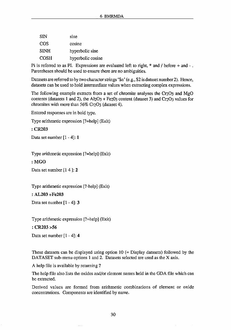
The following example extracts from a set of chromite analyses the Cr203 and MgOcontents (datasets 1 and 2), the Al203 + Fe203 content (dataset 3) and Cr203 values forchromites with more than 56% Cr203 (dataset 4).

Entered responses are in bold type.

Type arithmetic expression [?=help] (Exit)

: CR203

Data set number [1 - 4]: 1


: MGO

Data set number [1 4]: 2

Type arithmetic expression [?-help] (Exit)

: AL203 +Fe203



: CR203 >56


These datasets can be displayed using option 10 (= Display datasets) followed by theDATASET sub-menu options 1 and 2. Datasets selected are used as the X axis.

A help file is available by returning ?The help file also lists the oxides and/or element names held in the GDA file which canbe extracted.

Derived values are formed from arithmetic combinations of element or oxideconcentrations. Components are identified by name.

30

6 BMRMDA

An example is:

(FE203-1-PE,0)/2 >50 <90.0

This creates a new concentration which is half the sum of the concentrations of theindividual components (in this case oxides). Any valid arithmetic expression is permitted,but only values in the given range are accepted. Previously calculated values held in otherdatasets can be referenced by using the two characters $n, where n is the dataset number.This enables holding of intermediate values in datasets.

Press Enter to continue.

6.2 EXTRACT STRUCTURAL FORMULAE INTO DATASETSThis option is used to extract cations (or any arithmetic combination of cations) calculatedfrom the oxide and element concentrations in the GDA file. The program calculatesstructural formulae on the basis of the number of oxygens specified in the GDA file. Anoption is available to specify calculation with or without ferric iron, but note that ferriciron can only be calculated if both oxygen and cation numbers are given on the GDA file.

The following is an example of the type of cation ratios commonly used in plotting ofchromian spinels.

Calculate Ferric [YIN] (N)? Y


: 100*Cr/(Cr+Al)

Dataset number [1 - 4]: 1


: 100*Mg/(Mg+Fe2+)



: Fe3+/(Cr+A1+Fe3+)



: Cr/(Cr+A1+Fe3+)Dataset number [1 - 4]: 4The calculation of ferric takes slightly longer to perform than the standard structuralformula.

Atomic ratios such as 1001Q(K+Na+Ca) (i.e., Or content), can be extracted and laterrenamed (in this example to 'Mol percent Or') using options provided under the plottingroutines.

31

6 BMRMDA

Extraction of combined oxide or element weight percent data, or other parameters, suchas stratigraphic height or structural formulae components, can be made by sequentialextraction using options 1 and 2 and storing the data as datasets 1-4. Data from previousextractions will be held in their designated datasets until overwritten by subsequentextractions or exit from the BMRMDA program.

6.3 EXTRACT PYROXENES INTO DATASETSThis option extracts,pyroxenes and calculates structural formulae on the basis of 6 oxygenatoms, estimates Fe+ assuming pyroxene stoichiometry (4 cations per 6 oxygen atoms),assigns cations to the various pyroxene sites (T, M1 and M2) and calculates in activityMg2Si206, following the method of Wood and Banno (1973).

Atomic ratios are calculated as follows:

Mg# .^100Mg/(Mg+Fe2+)Ca* =^100Ca/(Ca+Mg+Fe)Mg* .^100Mg/(Ca+Mg+Fe)Fe*^=^100Fe/(Ca+Mg+Fe)WO" =^100Wo/(Wo+En+Fs)EN" =^100En/(Wo+En+Fs)FS"^=^100Fs/(Wo+En+Fs)ACF2 =Â1(M1)+Cr+Fe3++2Tiln(a)En =^log activity enstatite

Wo, En and Fs are calculated after the other end-members in the order given below.

The program also calculates the molecular percentage of the end members:

NaCrSi206^(Ureyite)ÛrCaCr2Si06^(Ca-Cr-tschermalcs) CaCrTsNaA1Si206^(Jadeite)^JdNaFe3+Si206 (Acmite)ÂcCaTiAl206^(Ca-Ti-tschermaks) CaTiTsCaAl2Si06^(Ca-tschermaks)^CaTsCaFe3+2Si06 (Ca-ferritschermaks) CaFeTsCaSiO3^(Wollastonite)^WoMgSiO3^(Enstatite)ÊnFeSiO3^(Ferrosilite)^Fs

End-members are calculated in the order listed following the method of Cawthorn andCollerson (1974), except that the Cr pyroxene components ureyite and Ca-Cr-tschermaksare calculated before jadeite.

The full list of cations, site allocations, atomic percentages and molecular percentages ofend-members, displayed under [?] help, is:

32

6 BMRMDA

Si Ti Al Cr Fe3+ Fe2+ Mn

Ni Mg Ca Na K Sum A112

An A1(M1) Mg(M1) (ACF2T) T(tot) Ml(tot) M2(tot)

ln(a)EN mg# Ca* Mg* Fe* WO" EN"

FS" Ur CaCrTs Ac Jd CaTiTs CaTs

CaFeTs Wo En Fs

This can be viewed by selecting the help option (?) when asked to type arithmeticexpression. Derived values may be formed by any arithmetic combination of the abovevalues.

6.4 EXTRACT AMPHIBOLES INTO DATASETSThis option extracts data from the GDA file and calculates structural formulae, as well asamphibole base end-members (Mol%) and site allocations. Estimation of ferric iron is bynormalising cations exclusive of Ca, Na, and K to 13, i.e., T + C = 13 (when Ca+Na>1.34), or by normalising the T + C + B exclusive of Na and K to 15 cations (when Ca+Na>1.34). The first option is generally preferable for most amphiboles, particularlycalciferous ones, whereas the normalisation to T + C + B = 15 is preferable for theanthophyllite - cummingtonite series.

Element names are:Si Ti Al Cr Fe3+ Fe2+ Mn

Ni Zn Mg Ca Na K A14

A16 FMM1 FMM4 CaM4 NaM4 NaA ATot

Mg# Fe3# Fe2" Anth Gedrite

Tremolite Hornblende Tschermak Winchite Barroisite Rieb+Glauc Na-anth

Na-Gedrite Edenite Parg+Hast Richterite Kataphor Taramite Arfv+Eck

Nyboite Kaersutite

where A14 and Al6 refer to tetrahedral and octahedral Al, respectively, FMM1 and FMM4are the sum of the ferromagnesian (Fe 2++Mg+Mn+Ni+Zn) cations in the M1 and M4,sites respectively, and NaA is the number of Na cations in the A site.

Mg#^100 Mg/(Mg+Fe2+)Fe3#^100Fe3+/(Fe2++Fe3+)Ca"^100Ca/(Ca+Mg+Fe2+)

100Mg/(Ca+Mg+Fe2+)Fe"^100Fe2+/(Ca+Mg+Fe2+)

and the end-member names refer to ideal end-member amphiboles.

Calculation of the amphibole end-members is based on the method of Currie (1991).

Amphiboles have the general formula A1-2B2C5T8022(OH,C1,F)2 where A = Na, K; B= Na, Li, Ca, Mn, Mg, Fe2+ ; C = Mg, Fe2+ , Mn, Al,^Ti ; T = Si, Al with other less

33

6 BMRMDA

common substitutions. The A, B and T-sites are used to classify 17 end-membermolecules (Hawthorne, 1983). Amphibole end-members are first classified into A-siteempty and A-site full types. End-members are then calculated according to Si6, Si7 andSig and B-site occupancy, with the B-site filled by FM, Ca or Na or mixed Na-Ca cations.

6.5 EXTRACT SPINELS INTO DATASETSIn this option spinels are extracted and their structural formulae are calculated on the basisof 4 oxygen atoms. Ideal end-member spinels are also calculated in the order listedfollowing a modified version of the method of Mitchell and Clarke (1976). An optionallows calculation of ferric iron assuming stoichiometry (i.e., 3 cations per 4 oxygens),depending on whether the oxidised or reduced spinel prism is selected.

For the oxidised prism the program calculates the following components (viewed usingthe help option).

Element names are:Mg#Âl/TriV^Cr/TriV^Fe3+/TriV Cr/(Cr+Al) SI^TI

AL^CR^FE3+^FE2+^MN^MG^NB

V^NI^ZN^CA^ZnAl204 MgAl204 FeAl204

MnAl204 Mg2TiO4 Mn2Ti 04 Fe2Ti 04 MgCr204 FeCr204^MnCr204

Fe304

where TriV = the sum of the trivalent cations (Al+Cr+Fe3+)/100.

For the reduced spinel prism only the following components are calculated, endmembers,apart from Fe304, being essentially the same (prior to normalisation)

Element names are:

Mg#Âl/TriV^Cr/TriV^2Ti/TriV Cr/(Cr+Al) SI^TI

AL^CR^FE2+^MN^MG^NB^V

NI^ZN^CA

where TriV = the sum of the tri-and quadrivalent cations (Al+Cr+2Ti)/100

6.6 EXTRACT GARNETS INTO DATASETSThis option allows garnet data to be extracted and structural formulae calculated on thebasis of 12 oxygen atoms. Calculation of ferric iron assumes stoichiometry (8 cations per12 oxygens). Selection can be made from concentration data, cations, cations in varioussites, and end-member garnet molecules as shown in the listing below (viewed using thehelp option).

Element names are:P205^Zr02^Si02^TiO2Âl203^Cr203^V203

Y203^Fe203^FeO^MnO^NiO^MgO^CaO

Na20^Total^P^Zr^Si^TiÂl

Cr^V^Y^Fe3+^Fe2+^Mn^Ni

34

6 B:rvIRMDA

Mg Ca Na Sum Ca* Mg* Fe*

MgNo# MgNo SiTET AITET TiTET Fe3+TET SUM

SiY AIY Fe3Y TiY V-Site X-Site Maj

Yt Ya Gold Kirnz Fe-Kirnz Uvar Knor

Sch And Py Sp Gr AIm Koh

Ski Cal Bly

Calculation of the garnet end-members is modified from the method of Rickwood (1968) to include majorite (maj). The full names and formulae of the end-members are given in 6.21. MgNo# and MgNo refer to 100MgI(Mg+Fe2+) calculated with FeO only and all Fe as FeO, respectively. Ca*, Mg*, and Fe* = 100 Ca/(Ca+Mg+Fe2+), etc.

6.7 SELECT GROUPS FOR DISPLAY This item allows selection of individual groups of samples within the data file.

Each of the groups is displayed in turn and selection is by responding yes or no.

6.8 DELETE ALL PLOT FILES All existing plot files (GDA1.VEC etc.) are deleted by this function. Care should be taken to ensure that a back-up copy is made of those plot files required for future plotting (replotting).

6.9 DEFINING PLOT PARAMETERS Item 9 on the MDA menu ('Define main plot parameters') is used to allocate symbols, pen colours, and line types to sample groups, and to define symbol, text, and axis dimensions. Commonly the default parameters may be adequate, but these may be changed and the plot parameters stored on a file for subsequent retrieval and re-use. Different parameters may be required for display on screens and on plotters.

The various optional parameters can be allocated using the following menu.

Default values are given in brackets.

MAIN PLOT PARAMETERS

(I) Retrieve plot parameters (from file)

(2) Change title text height (1.5cm)

(3) Change axes labels text height (1.0cm)

(4) Change sample numbers and points text height

(5) Change symbol height (0.5cm)

(6) Change axes tick height (1.0cm)

(7) Change font (0.5)

(8) Change group pens

35

6 BMRMDA

(9) Change group symbols

(10) Change group linetypes (1)

(11) Change axes pen (1)

(12) Change titles pen (1)

(13) Change histogram pen (1)

(14) Change plot title

(15) Change legend symbol and text heights (1.0)

(16) Change axes lengths (X = 25.0cm; Y = 20.0cm)

(17) Define metafile path & preceding characters in name

(18) Store plot parameters (on file)

Option [1 - 17] (Exit):

An example of a plot parameters file is given in the GDA manual. Normally the formatwill not be of interest to the user as it will not be necessary to edit such a file.

There are choices of up to 8 pens (depending on the type of plotter), 15 symbols, 6linetypes and 15 fonts (15 - 19 are the same), all of which may be displayed on screen byselecting the display option (?). As default values for these, pen 1 and symbol 1 areassigned to group 1, pen 2 and symbol 2 to group 2, and so on. Pens and symbols assignedto each group may be checked by displaying the legend. The default linetype for allgroups is 1 (solid line); note that the linetypes as displayed on the screen may be slightlydifferent from those used by the plotter.

The symbols, linetypes and fonts are shown in Figures 1-4 in the GDA manual.

The default axis lengths (25 x 20cm) produce a plot of that size on the plotter, and areduced plot on the screen. The size and shape of the final plot (triangular plots excepted)may be changed by changing the axis lengths, but note that the maximum plot size(including axis labels) for an A3 page plotter is about 40 x 28cm and that such a plot sizewould overflow the screen. However, this option can be useful in arranging more thanone plot on a single page (see under VECTOR). The default symbol and text sizes areappropriate for standard size plots, but may need changing if the axis lengths are greatlychanged. The numbers of axis labels and ticks on each axis are set automatically andcannot be selected by the user. However, the numbers will be reduced if plots are stackedor reduced in size. It is possible to set the tick size to zero, and add the required numberof ticks by hand.

Item 17 (define metafile path and preceding characters in name) allows plot metafiles tobe written to a different drive (such as a floppy disk) or directory. The latter may be usefulfor a networked system. The specified path is added to the beginning of the plotfile name,but take care not to specify a non-existent directory. For example:

36

6 BMRMDA

• C:\xxx\ would write the metafile to directory xxx on drive C (e.g.,

C:\xxx\GDA1.VEC);

• A: (or A:\) would write the metafile to floppy disk drive A (e.g., A:\GDA1.VEC);

• AB would add AB to the metafile name (e.g., ABGDA1.VEC);

• D:\GDB\AB would write the metafile to directory GDB on drive D and add the prefix AB (e.g., D:\GDB\ABGDA1.VEC).

The default is set so that the metafile is written to the current (Le., GDA) directory.

6.10 DISPLAY DATASETS This option enables one or more datasets to be displayed on an XY plot of value against sample order in the dataset. Each sample group is displayed sequentially, using the appropriate symbol and pen colour. Either a single dataset (e.g., element) may be displayed, or plots of up to 4 datasets may be stacked.

The menu is as follows:

(1) Display (either on screen or metafile; plot number (1-99) must be specified in latter case)

(2) Select datasets (e.g., elements) for display (if more than one is selected, plots will be stacked)


(4) Change axes titles (for any selected dataset)

(5) Display sample numbers (on plot)

(6) Set axes extremes to data range plus 20%

(7) Set axes extremes to nice limits (this is the default which selects a logical whole-number range for each axis, depending on which groups are se lected for display)

(8) Set axes extremes to typed-in values (any values may be selected, but note that they will also apply to histograms and XY plots (but not triangular plots»

(9) Set log or linear axes (for any selected dataset)

(10) Define pen for mean lines (0): (1 of up to 8 colours; displays mean for all groups selected for display in 13)

(11) Define pen for median lines (0) (as 10)

(12) Define pen for standard deviation lines (O)(as 10)

(13) Select groups to be displayed (any or all assigned groups may be displayed on each plot)

(14) Specify additional plot points and/or text

37

6 BIVIRMDA

Additional plot points or text such as a legend, may be added to previously selected plotsvia the keyboard. The following must be given:

• X, Y co-ordinates (separated by a comma; previously specified points ortext will be deleted if no values are entered here; co-ordinates outside theplotting area are permissible)

• Pen number• Symbol number (if none is given, only text will be output)• Text (e.g., sample number or a legend; 0 - 50 characters)• Y - axis dataset (this number must be specified for each extra point or text

required; for stacked plots, points or text may be added to any plot byspecifying the appropriate dataset).Note that the given XY co-ordinates define the centre of the symbol or, ifno symbol is specified, the bottom of the first character of text. All addedpoints or text required for a given plot (either single or stacked) must bespecified in one operation (as previously added points will be replaced whenthis option (14) is selected a second time); the maximum is 20 extra pointsand/or text lines).

(15) List statistics (includes minimum, maximum, mean, median, standard deviation,skewness, and kurtosis; calculated for all samples in the selected groups andfor selected datasets; if log axes are selected, statistics will be calculated usingnatural log values).

The statistics are displayed, and are also listed on a file MDA.PRN, which maysubsequently be printed (and edited if required)

6.11 DISPLAY HISTOGRAMSHistograms of three types may be displayed - for single datasets, stacked for up to 4datasets, or stacked for selected groups for a single dataset (see item 13). The menu issimilar to that for display of datasets:

(1) Display (on screen or metafile 1-99)

(2) Select datasets (e.g., elements for display)


(4) Change axes titles


(6) Set axes extremes to nice limits

(7) Set axes extremes to typed-in values

(8) Define histogram box width

(9) Define pen for mean lines

(10) Define pen for median lines

(11) Define pen for standard deviation lines

38

6 BMRMDA

(12) Select groups to be displayed

(13) Select histogram type

• Single element (for selected groups)• Stacked for selected datasets (for all selected groups)• Stacked groups for one dataset (each selected group is plotted separately

with group numbers at right)

(14) Specify additional plot points and/or text (for histograms, this option is mainlyuseful for adding text, such as a legend, to a previously selected plot):

• X, Y co-ordinates (separated by a comma; if no values are entered,previously specified points or text will be deleted)

• Pen number• Symbol number (if none is given, only text will be output)• Text (e.g., a legend; 0 - 50 characters)• Y-axis dataset (this specifies the dataset selected for a single histogram

(actually the X-axis in this case), or for any dataset on a stacked plot ofdatasets)OrGroup number (this specifies the group for a stacked plot of groups for onedataset)Note: the given XY co-ordinates define the centre of the symbol or, if nosymbol is specified, the bottom of the first character of text. The maximumnumber of added points and/or text lines is 20. All those required for a givenplot (either single or stacked) must be specified in one operation).

(15) List statistics (for all samples in the selected groups and for selected datasets;may be printed from file MDA.PRN).

An example of a histogram used to portray garnet compositions from two of the Wandageealkaline ultrabasic pipes in Figure 1.

39

FIG. 1. STACKED HISTOGRAM OF GARNET COMPOSITIONS

••••lIl-

4Frequency

1

-

.11

-

1•11■1

-

-_

MN

IIIMOI

.1M.

41•11

■11-=I

.1=1

■Il

.1.

_MIWO

6 BMRMDA

6.12 DISPLAY XY PLOTAs for datasets and histograms, plots may be single or stacked. Menu items 1 - 12 areidentical to the display dataset menu. Because of memory limitations options 13 and 19on the GDA menu - least squares line fitting and least squares lines for individual groupsare not available for MDA. The remainder are as follows:

(14) Define pen for regression polygons (different colours may be specified for 1st,2nd and 3rd order regressions, calculated for all selected groups, using eithervalues or log values)


(16) Specify additional plot points and/or text (additional points or text, such as alegend, may be added to previously selected plots via the keyboard

• X, Y co-ordinates (separated by a comma; previously specified points ortext will be deleted if no values are entered here)

• Pen number• Symbol number (if none given, only text will be output)• Text (e.g., sample number or a legend; 0 - 50 characters)• Y-axis dataset (this must be specified for each extra point or text required;

for stacked plots, points or text may be added to any plot by specifying theappropriate dataset).Note: the given XY co-ordinates define the centre of the symbols or, if nosymbol is specified, the bottom of the first character of the text. If a newX-axis dataset is selected the added points may still appear, so be sure todelete any additional points (by choosing option 16 again, but not enteringany XY co-ordinates) before selecting new datasets for display. All addedpoints or text required for a given plot (either single or stacked) must bespecified in one operation; the maximum number of added points and/ortext lines is 20).

Specify graphics overlay files (lines and/or text may be added by selecting an appropriatefile - see appendix C for details of format and available files; make sure that the X and Ydatasets are correct and the axis extremes are appropriate; the Y-axis dataset and name ofthe graphics overlay file (????.GRF) must be given)

(18) Regression curves for individual groups (as 14, except that curves are calculatedseparately for each displayed group)

(20) List statistics (comprises minimum, maximum, mean, median, standarddeviation, skewness, kurtosis, correlation coefficient, and 1st, 2nd, and 3rdorder regression coefficients, standard deviations, and T-values; calculated forall samples in the selected groups and for selected datasets or pairs of datasets(X with each Y); if log axes are selected for any dataset(s), statistics will becalculated using the natural logarithms of those dataset values; if regressioncurves for individual groups are specified (18), statistics for each selected groupwill also be listed; results may be printed from file MDA.PRN)

41

6 BMRMDA

An example of an XY plot showing the composition of diamond facies chrome spinels is shown in Figure 2 and the corresponding statistics printout is given in Table 1.

TABLE 1. STATISTICAL DATA FOR FIGURE 2.

XY PLOT OF DIAMOND FACIES CHROMITES

100Mg/(Mg+Fe2+)

Minimum: Maximum: Mean: Median Standard Deviation: Skewness: Kurtosis:

100Cr/(Cr+Al)

Minimum: Maximum: Mean: Median Standard Deviation: Skewness: Kurtosis:

Regression Statistics:

2.8740 79.4540 60.6240 62.6530 14.8066 -l.8929 5.4445

82.8660 95.7810 89.0946 88.7500

2.8370 .4491 .3798

Independent Variable: 100Mg/(Mg+Fe2+) Dependent Variable: 100Cr/(Cr+Al)

Correlation Coefficient: -.5204 Product-Moment Correlation Coefficient based on 61 pairs of values: -.5204

Polynomial of degree 1 Standard error: 2.4 Regression Coefficient(s): 95.14 -.9972E-01 Coefficient(s) Standard Deviation: .2130E-01 T-Value(s): -4.682

Polynomial of degree 2 Standard error: 2.4 Regression Coefficient(s): 92.92 .1701E-01-.1249E-02 Coefficient(s) Standard Deviation: .7103E-01 .7262E-03 T-Va1ue(s): .2396 -1.720

Polynomial of degree 3 Standard Regression Coefficient(s): Coefficient(s) Standard Deviation: T-Value(s):

error: 9l.45 .2437 l.473

42

2.4 .3589 -.1103E-01 .6711E-02 .5009E-04

-l.643 l.465

. 7340E - 04

FIG. 2. XY PLOT OF DIAMOND FACIES CHROMITES

AAAA

• 90 • ~~ . ... ~ .4~t

~ A .-«

+ 80 "- 0-

U 0; "--/ ~ ~

"" w :;0

"- ~ u • Chromite inclusions • diamond

t:J 70 In >

0 0 or-

60 A Chromite-diamond intergrowths

20 40 60 80 100Mg/ (Mg+F e2+)

6 BMRMDA

6.13 DISPLAY TRIANGULAR PLOTAny 3 datasets may be selected for display on a triangular plot.

(1) Display (on screen or metafile 1 - 99)

(2) Select datasets (e.g., elements) for display

(3) Change plot title (previous title is deleted if nothing is entered)

(4) Change apex titles

(5) Display sample numbers


(7) Specify additional plot points and/or text (additional plot points or text, such asa legend, may be added to previously selected plots via the keyboard; thefollowing must be given:

• X, Y, Z co-ordinates (separated by commas; either straight elementconcentrations or normalised co-ordinates (i.e., totalling to 100) may beused; previously specified points or text will be deleted if no values areentered here; co-ordinates outside the plotting areas (i.e., negative) arepermissible, but obviously must be adjacent to the plot)

• Pen number• Symbol number (if none is given, only text will be output)• Text (e.g., sample number or a legend; 0 - 50 characters)

Note that the given XYZ co-ordinates define the centre of the symbol or, ifno symbol is specified, the bottom of the first character of text. All addedpoints or text required for a given plot must be specified in one operation;the maximum number of added points and/or text lines is 20. To align 2 ormore lines of text vertically - for each unit decrease in the Y co-ordinate,increase X and Z by 0.5 units each).

(8) Specify graphics overlay files (xxx.GRF)

An example of a triangular plot showing the composition of garnets from two of theWandagee alkaline ulft-abasic pipes is given in Figure 3.

44

FIG. 3. XYZ PLOT OF GARNET COMPOSITIONSMgO wt %

•Pipe M89 garnets

*Pipe M97 garnets

v./^\iv

CaO wt %^ Cr203 wt %

6 BMRMDA

6.14 DISPLAY LEGEND This may be used to display the symbols and the pen colours assigned to sample groups. It may be written to a metafile so that the legend may be output to a plotter.

6.15 DISPLAY SPINEL PRISM This option allows spinel compositions to be plotted in the spinel prism (Irvine, 1965). Projections can be made into either the oxidised prism in terms of (MgFe)AI204-(MgFe)C1'204-(MgFe)Fe204 with Fe3+ calculated from stoichiometry or the reduced prism in terms of (MgFe)A1204-(MgFe)C1'204-(MgFe)2Ti04 with all Fe assumed to be Fe2+. The latter is useful for kimberlite spinels which formed under relatively reducing conditions.

The submenu is

SPINEL PRISM

(1) Display (on screen or metafile 1-99)


(3) Display sample numbers


Examples of the spinel prism plots for both the oxidising and reduced prisms are shown in Figure 4. Note that for the oxidised prism, the symbol size is scaled according to the Ti02 content of the spinel: spinels with higher Ti02 contents are plotted using smaller symbols, because such compositions generally occur in more evolved rocks and are relatively fine-grained.

46

0.2

0.4

0.6

0.8

MgAl204

FIG. 4A. OXIDISED SPINEL PRISM PLOTFe304

0.80.6

FeCr204

MgCr204

FIG. 4B. REDUCED SPINEL PRISM PLOTFe2TiO4

0.8

FeCr204

MgCr204

6 BMRMDA

6.16 DISPLAY BOX-WHISKER PLOT

Box-whisker plots may be used to display many datasets on a single diagram together with mean and standard deviation boxes for each dataset. Such plots are useful for highlighting anomalous values and for making comparisons with average data. The box-whisker menu is:

BOX-WHISKER PLOT

(1) Display



(4) Set axes extremes to nice limits

(5) Set axes extremes to typed in values


(7) Select box-whisker type

(8) Specify additional plot points and/or text

(9) Specify box size

(10) Display box

(11) Display samples inside box

(12) Linear / log axis

(13) Define pen for box

Option [1-13] (Exit):

Options 1-8 are similar to the options available for histogram plots. Option 9 is used to specify box size (0-5 standard deviations above and below the mean; default is 1.0). Option 10 enables the boxes to be omitted if desired, with option 11 the sample points inside boxes may be omitted, option 12 defines linear or log axes, and option 13 offers a choice of pen colours for the box.

The default Box-whisker Plot Definition File (BOXWHISK.DEF) comprises the major oxides. Suitable mineral reference files may be set up and expressions as well as concentrations incorporated as required. An example of the box-whisker plot to show compositional variation amongst chrome spinel inclusions in diamond is shown in Figure 5.

49

FIG. 5. BOX-WHISKER PLOT OF CHROMITES IN DIAMOND

30.0 , ... -

ffi EE 10.0 +J EIJ c ... (l) ... t

0\

() OJ Ul L.. 3.0 • • I ~ 0 (l) ~ a.. 0 ... >-

+J • ..c 1.0 Ol l .-Q) ... 3: ...

0.3 ...

0.1

Ti02*10 Cr203 FeO NiO*10 ZnO*10 AI203 V203*10 MnO*10 MgO

6 BMRMDA

6.17 PRINT STRUCTURAL FORMULAE REPORT This option generates on file MDA.PRN a table of analyses and atomic proportions calculated using the number of oxygens and cations stored in the GDA data file. Ferric iron will only be calculated if non-zero values are held in both the cations and oxygens fields. The sample number, analysis number and mineral description fields are printed at the bottom of the table. An example is given in Table 2. The file MDA.PRN may be modified using a text editor prior to printing.

TABLE 2. EXAMPLE OF STRUCTURAL FORMULAE REPORT

STRUCTURAL FORMULAE - crnod.GDA

A B C D E MgO 12.82 15.42 14.84 14.70 14.72 A1203 7.88 14.02 14.27 13.60 10.40 Si02 .06 <.02 .03 .03 <.02 CaO <.02 <.02 <.02 <.02 <.02 Ti02 .10 .11 .20 .21 1.73 V203 .17 .00 .30 .28 .23 Cr203 64.68 57.49 57.59 57.63 57.53 MnO .16 .12 .12 .09 .14 Fe203 .54 2.84 1. 05 1. 56 3.00 FeO 13.60 10.80 11.61 11.62 12.46 NiO .07 .13 .10 .14 .19 ZnO .11 .00 .06 .07 .09 Total 100.18 100.93 100.17 99.94 100.49

Atomic Proportions.

Ox 4.0000 4.0000 4.0000 4.0000 4.0000 Mg .6241 .7151 .6940 .6915 .6989 A1 .3033 .5141 .5277 .5059 .3904 Si .0020 .0009 .0009 Ti .0025 .0026 .0047 .0050 .0414 V .0045 .0075 .0071 .0059 Cr 1. 6702 1.4142 1. 4287 1.4381 1.4488 Mn .0044 .0032 .0032 .0024 .0038 Fe+++ .0132 .0666 .0248 .0371 .0720 Fe++ .3714 .2811 .3045 .3068 .3318 Ni .0018 .0033 .0025 .0036 .0049 Zn .0027 .0014 .0016 .0021 Total 3.0000 3.0000 3.0000 3.0000 3.0000

A: AR2/1 AVERAGE 8 CHROMITE CORES B: N38/1 CHROMITE CORE C: N41/1 AVERAGE 8 CHROMITE CORES D: N45/1 AVERAGE 14 CHROMITE CORES E: N45/2 CHROMITE RIM

51

6 BMRMDA

6.18 PRINT PYROXENES REPORTThis option generates, as a print file (MDA.PRN), a report of pyroxene analyses includingstructural formulae calculated on the basis of 4 cations per 6 oxygens. Site occupancyfollowing the method of Wood and Banno (1973), atomic ratios (Ca/(Ca+Mg+Fe), etc.),and percent end member molecules. The pyroxene structure is examined for conformityto the ideal pyroxene formula and the program gives warnings if the number of oxygensin the formula sums to less than 6 or if any of the following rejection criteria apply:

• Si>2.02 or<1.98

• ACF2T - Ti + Mg + Fell- + Fe3+ + Mn + Ni <0.98, whereACF2T = A1M1 + Cr + Fe3+ + 2Ti

• Sum of M2 cations <0.98 or> 1.02

• ACF2T - Ca - Na - K - Ally >0.030

• Na >ACF2T

The percentage of pyroxene end-member components are calculated in the orderNaCrSi206 (ureyite), CaCr2Si06 (Ca-Cr-tschermaks), NaA1Si206 (jadeite),NaFe3+ Si206 (acmite), CaTiAl206 (Ca-Ti-tschermaks), CaAl2Si06 (Ca-tschermaks),CaFe3+2Si06 (Ca-ferritschermalcs), CaSiO3 (wollastonite), MgSiO3 (enstatite) andFeSiO3 (ferrosilite) following a modified version of the method suggested by Cawthornand Collerson (1974). The remaining unassigned cations are listed. For good qualityanalyses the percentage of unassigned cations should be less than 1%. The print fileMDA.PRN may be printed direct or modified by word processor.

An example of the pyroxene report is given in Table 3.

52

6 BMRMDA

TABLE 3. EXAMPLE OF PYROXENE REPORT

-----------------------------------------------------------------------------

E9/8/l Cpx -----------------------------------------------------------------------------oxides: analysis: ferric: cations: site occupancy:

Si02 54.69 54.69 Si 1. 965 1. 963 Al/2. .193 .192 Ti02 .68 .68 Ti .018 .018 A1(T) .035 .037 A1203 9.10 9.10 Al .385 .385 Al(M1) .350 .348 Cr203 .05 .05 Cr .001 .001 Mg(M1) .459 .459 Fe203 .00 .46 Fe3+ .000 .012 (ACF2T) .388 .398 FeO 6.30 5.89 Fe2+ .189 .177 T(tot) 2.000 2.000 MnO .12 .12 Mn .004 .004 M1(tot) 1.000 1.000 NiO .00 .00 Ni .000 .000 M2(tot) 1.004 1.000 MgO 9.44 9.44 Mg .506 .505 In(a)EN -3.680 -3.644 CaO 14.93 14.93 Ca .575 .574 mgfl: 72.8 74.1 Na20 4.85 4.85 Na .338 .337 K20 .51 .51 K .023 .023 Total 100.67 100.72 Sum 4.004 4.000

atomic ratios: Ca* 45.3 Mg* 39.8 Fe* 14.9

no ferric: WO" 44.7 EN" 40.2 FS" 15.1 ---accepted 0 warning(s) ferric: WO" 44.7 EN" 40.9 FS" 14.3 ---accepted 0 warning(s)

Molecular Percent End-members

NaCrSi206 (Ureyite) Ur .14 GaGr2Si06 (Ga-Gr-tschermaks) CaGrTs .00 NaA1Si206 (J adei te) Jd 36.04 NaFe+++Si206 (Acmite) Ac .00 CaTiA1206 (Ca-Ti-tschermak) GaTiTs 1. 28 CaA12Si06 (Ca-tschermak) GaTs .00 GaFe+++2Si06 (Ca-ferritschermak) CaFeTs .62 CaSi03 (Wo llas toni te) Wo 27.83 MgSi03 (Enstatite) En 25.32 FeSi03 (Ferrosilite) Fs 8.76 Remaining Ti .006 Remaining Fe2+ .006 Percentage of unassigned cations is .28

53

6 BMRMDA

6.19 PRINT AMPHIBOLES REPORT

This option allows calculation of amphibole end members in molecular percentages and the site allocations. It also provides an estimate of Fe203 content for microprobe analyses by normalisation of the the cations to either

• T + C = 13.0 exclusive of Ca, Na and K (recommended for the majority of

amphiboles, especially calciferous varieties where Ca+Na> 1.34)

or

• T + C + B = 15.0 exclusive of Na and K (recommended for Fe-Mg-Mn

amphiboles).

The program calculates end members based on the 17 end-member amphiboles recognised by Hawthorne (1983), following a modified form of the method proposed by Currie (1991). The report is generated under MDA.PRN which can be edited and printed. The following end-member amphiboles are calculated:

Anthophyllite, gedrite, tremolite, hornblende, tschermakite, winchite, barroisite, NazFM3MzSi80ZZ (riebeckite-glaucophane), Na-anthophyllite, Na-gedrite, edenite, NaCazFM4M3Si60ZZ (has tingsi te-pargasite), richteri te, ka ta phorite, taramite, Na3FM4MSi80ZZ (arfvedsonite-eckermannite), nyboite and kaersutite.

The amphibole structure is examined for conformity to the ideal amphibole structure and rejects analyses which violate the following conditions:

• Si + Ai <8.00

• Si >8.00

• Ml cations >5.00, i.e., Cr + Alvi+Fe3+Ml + Ti >5.00

• Ca >2.00

• M4 site cation deficient

• Ca required in A-site

• A-site cations> 1.00.

An example printout is given in Table 4.

54

6 BMRMDA

TABLE 4. EXAMPLE OF AMPHIBOLE REPORT

AMPHIBOLES REPORT - wandamph.GDA

VJANDAGEE/31475 AMPHIBOLE 3 GEN 256

oxides all FeO: ferric: cations: Site allocation:

Si02 41. 62 41. 62 Si 6.188 6.077 Si 6.188 6.077 Ti02 .74 .74 Ti .083 .081 A14 1. 812 1. 923 A1203 13.92 13.92 A1 2.440 2.396 Fe3 .000 .000 Cr203 .05 .05 Cr .006 .005 8.000 8.000 Fe203 .00 7.53 Fe3+ .000 .827 A16 .629 .473 FeO 14.23 7.46 Fe2+ 1.770 .911 Ti .083 .081 MnO .38 .38 Mn .048 .047 Cr .006 .005 NiO .00 .00 Ni .000 .000 Fe3 .000 .827 ZnO .00 .00 Zn .000 .000 Fe-Mg 4.283 3.613 MgO 12.19 12.19 Mg 2.703 2.654 5.000 5.000 CaO 9.95 9.95 Ca 1. 586 1. 557 Fe-Mg .238 .000 Na20 3.84 3.84 Na 1.107 1. 087 Ca 1.586 1. 557 K20 1. 35 1. 35 K .257 .252 Na .176 .443 Total 98.28 99.04 Sum 16.188 15.897 2.000 2.000

Na .931 .645 , \

K .257 .252 1.188 .897

Total 16.188 15.897

Mg# 60.4 74.5 all FeO analysis: ***rejected 1 error(s) Fe3# .0 47.6 ferric analysis: ---accepted 0 error(s) Ca" 26.2 30.4 Mg" 44.6 51. 8 Fe2" 29.2 17.8

End-members (Mol fraction) Fe-Mg amphibole .000 Ca-Na amphibole 1.000 A-site vacant

Hornblende .0019 ferri- .0012 a1umino- .0007 Tschermakite .0556 ferri- .0353 a1umino- .0202 Barroisite .0456 ferri- .0290 a1umino- .0166

A-site full Edenite .0386 ferri- .0245 alumino- .0140 NaCa2FM4MSi6A12 .3802 Hastingsite .2418 Pargasite .1384 Kataphorite .0306 ferri- .0195 a1umino- .0111 Taramite .3663 ferri- .2330 a1umino- .1333 Kaersutite .0812 ferri- .0516 a1umino- .0295

55

6 BMRMDA

6.20 PRINT AMPHIBOLE CLASSIFICATION REPORT This option employs the program AMPHTAB (Rock, 1987) to calculate amphibole formula units and classify and name amphiboles according to the lMA (1978) scheme.

Options are available for calculation of Fe3+ and for inclusion and treatment of H20, C02 and P20S contents. An example of output is given in Table 5 and full details are given by Rock (1987).

TABLE 5. EXAMPLE OF AMPHIBOLE CLASSIFICATION REPORT

Classify amphiboles using IMA(1978) scheme [Mineral.Mag.42,533-63)

GDA file: wandamph.GDA

1 2 3

Si02 40.73 4l. 35 4l. 62 Ti02 .67 .37 .74 A1203 16.33 15.20 13.92 Cr203 .03 .10 .05 Fe203 .00 .00 .00 FeO 12.79 12.28 14.23 MnO .23 .27 .38 MgO 11.28 12.51 12.19 \ \

CaO 10.93 10.00 9.95 Na20 3.58 4.02 3.84 K20 .86 1. 30 1. 35

TOTAL 97.43 97.41 98.37

CATIONS PER FORMULA UNIT 0= 23.0 23.0 23.0 Si 6.002 6.055 6.077 Al 2.837 2.623 2.396 Fe3+ .369 .650 .827 Fe2+ l. 207 .853 .911 Mg 2.478 2.731 2.655 Ca 1.727 1.569 l. 557 Na 1.022 1.141 1. 087 K .162 .244 .252 Ti .074 .041 .081 Mn .029 .034 .047 Cr .003 .012 .005

TOTAL 15.911 15.953 15.897

CHECK ON OXYGEN(+C1,F) EQUIVALENCE OF ABOVE CATIONS 0= 23.00 23.00 23.00

IMA(1978) CLASSIFICATION PARAMETERS CaNa 2.000 2.000 2.000 NaB .273 .431 .443 NaKA .911 .953 .897 AIVI .839 .678 .473 MgFe .672 .762 .745

56

6 BMRMDA

TABLE 5. CONTINUED

GENERAL NOTES FOR THE ABOVE TABLE: P205 (where quoted) has been treated as zero in calculation of formula unit. Results have not been checked or adjusted for low water/high cation totals. Fe has been reallocated wherever possible between Fe3 and Fe2, where only total Fe is quoted.

IMA(1978)Names for the above Table:

Analysis: WANDAGEE/3l473 Number: 1 Sum of cations S2 brought to 13.0 by redistribution of total Fe between Fe2 & Fe3

SODIAN FERROAN PARGASITE

Analysis: WANDAGEE/3l474 Sum of cations S2 brought to total Fe between Fe2 & Fe3

SODIAN PARGASITE

Analysis: WANDAGEE/3l475 Sum of cations S2 brought to total Fe between Fe2 & Fe3

POTASSIAN SODIAN MAGNESIO-HASTINGSITE

Number: 2 13.0 by redistribution of

Number: 3 13.0 by redistribution of

57

, \

6 BMRMDA

6.21 PRINT SPINELS REPORT

Option 6.21 generates on the MDA print file (MDA.PRN) a report of spinel compositions with ferric contents calculated assuming 3 cations for 4 oxygens. Spinel end-numbers are calculated in the order ZnAh04, MgAh04, Mg2Ti04, Mn2Ti04, Fe2Ti04, MgCr204, , MnCr204, FeCrz04, and Fe304 following a modified version of the method of Mitchell and Clarke (1976). An example of the output is given in Table 6.

58

6 BMRMDA

TABLE 6. EXAMPLE OF SPINEL REPORT

SPINELS REPORT - sp1herz.GDA

Analysis 75210425A2/1 SPINEL Wt % 0= 4.0 ppm

MgO 19.03 A1203 43.33 Si02 .07 CaO <.02 Ti02 .47 V203 .08 Cr203 24.17 MnO .07 Fe203 2.97 FeO 9.96 NiO .30 ZnO .12 Total 100.57

Reduced 100Mg/(Mg+Fe) 100A1/(Al+Cr+2Ti) 100Cr/(Al+Cr+2Ti) 200Ti/(A1+Cr+2Ti) 100Cr/(Cr+Al)

End members ZnA1204 MgA1204 FeA1204 MnA1204 Mg2Ti04 Mn2Ti04 Fe2Ti04 MgCr204 FeCr204 MnCr204 Fe304

.242 69.408

.000

.000 1.155

.000

.000 6.311

19.678 .162

3.044

.7737 1. 3930

.00l9

.0096

.0017

.5213

.0016

.0609

.2272

.0066

.0024 3.0000

72 . 866 72.044 26.959

.997 27.231

114771 229324

327 <143 2818

544 165372

542 20748 77426

2358 964

Oxidised 100Mg/(Mg+Fe2+) 100A1/(Al+Cr+Fe3+) 100Cr/(Al+Cr+Fe3+) 100Fe3+/(Al+Cr+Fe3+) 100Cr/(Cr+A1)

59

77 . 299 70.526 26.391

3.083 27.231

6 BMRMDA

6.22 PRINT GARNET REPORT This option generates a report on garnet analyses as a print file (MDA.PRN), which may be output direct to a printer or first modified by word processor. The program allocates cations to sites, calculates ferric iron assuming 8 cations for 12 oxygens, and calculates garnet end-member components in the order NaCa2AISi4012 (Majorite), Y3Al2A13012 (Yttrogarnet), Mn3 V2Si3012 (Y amatoite), Ca3 V2Si3012 (Goldmanite), Ca3ZrzAl2Si012 (Kimzeyite), Ca3Zr2Fe3+Si012 (Ferric-Kimzeyite), Ca3Cr2Sb012 (Uvarovite), Mg3Cr2Sb012 (Knorringite), Ca3TizFe3+Ti012 (Schorlomite), Ca3Fe3+2Sb012 (Andradite), Mg3Al2Sb012 (Pyrope), Mn3Al2Sh012 (Spessartine), Ca3Al2Sh012 (Grossular), Fe2+ AIzSb012 (Almandine), Mg3Fe3+2Sb012 (Koharite), Fe2+Fe3+ 2Si3012 (Skiagite), Mn3Fe3+ 2Sb012 (Calderite), and Mn2+ 3Mn3+ 2Sb012 (Blythite), following a modified form of the method of Rickwood (1968). Remaining cations should be less than 1 % for a good analysis. The common garnets are classified and named according to the Dawson and Stephens (1975) classification scheme. An example of output is given in Table 7.

60

6 BMRMDA

TABLE 7. EXAMPLE OF GARNET REPORT

GARNET REPORT - akconga.GDA

ARGYLE/31382 CONCENTRATE LDC 0-4-12 -----------------------------------------------------------.-----------------

oxides: analysis: ferric: cations: site occupancy:

P205 .04 .04 P .002 .002 SiTET 2.984 2.973 Zr02 .00 .00 Zr .000 .000 A1TET .016 .027 Si02 42.06 42.06 Si 2.981 2.970 TiTET .000 .000 Ti02 .70 .70 Ti .037 .037 Fe3+TET .000 .000 A1203 2l. 59 2l. 59 A1 1.804 1.797 SUM 3.000 3.000 Cr203 l. 81 l.81 C'r .101 .101 SiY .000 .000 V203 .00 .00 V .000 .000 A1Y 1.787 1.770 Y203 .00 .00 Y .000 .000 Fe3Y .000 .088 Fe203 .00 l. 66 Fe3+ .000 .088 TiY .037 .037 FeO 7.40 5.91 Fe2+ .439 .349 Y-Site l. 926 l.996 MnO .24 .24 Mn .014 .014 X-Site 3.104 3.004 NiO .00 .00 Ni .000 .000 MgO 21. 93 21. 93 Mg 2.317 2.309 CaO 4.28 4.28 Ca .325 .324 Na20 .06 .06 Na .008 .008 Total 100.11 100.28 Sum 8.029 8.000

atomic ratios: Ca* 10.5 Mg* 75.2 Fe* 14.2 . " \ \

100Mg/(Mg+Fe2+): 86.9

100Mg/(Mg+Fe): 84.1

Molecular Percent End-members

NaCa2A1Si4012 (Maj orite) Maj .82 Y3A12A13012 (Yttrogarnet) Yt .00 Mn3V2Si30l2 (Yamatoite) Ya .00 Ca3V2 S i3012 (Go ldmanite) Gold .00 Ca3Zr2A12Si012 (Kimzeyite) Kimz .00 Ca3Zr2Fe3+2SiOI2(Ferric-Kimzeyit Fe-Kimz .00 Ca3Cr2Si3012 (Uvarovite) Uvar 5.07 Mg3Cr2Si3012 (Knorringite) Knor .00 Ca3Ti2Fe3+2Ti012(Schor1omite) Sch l. 24 Ca3Fe3+2Si3012 (Andradite) And 3.18 Mg3A12Si3012 (Pyrope) Py 77 .17 Mn3A12Si3012 (Spessartine) Sp .48 Ca3A12Si3012 (Grossular) Gr .79 Fe2+A12Si30l2 (Almandine) AIm 11.25 Mg3Fe3+2Si30l2 (Koharite) Koh .00 Fe2+3Fe3+2Si30l2 (Skiagite) Ski .00 Mn3Fe3+2Si30l2 (Calderite) Cal .00 Mn2+3Mn3+2Si30l2 CBlythite) Bly .00 Remaining Si .010 Remaining Fe2+ .012 Percentage of unassigned cations is .28

Dawson & Stephens - group no 1 Titanian pyrope

61

7 VECTOR

Plot (i.e., graphics) files generated in BMRMDA (generally with names between GDA1.VEC and GDA99.VEC) using the SciPIot Graphics package can be output to various devices, either directly, or,for some plot file types, using the VECTOR program. A number of different graphics file types is available, and the one required must be specified when generating plot files in BMRMDA (see above). However, plotter and printer meta files may be output to either device (although the size may need changing), or displayed on screen. Examples of mineral plots generated in BMRMDA and output to laser printer from HPGL files are given in Figures 1 - 8.

The Postscript file is an ASCII file·that may be edited or sent directly to any Postscript printer. The Encapsulated Postscript file (EPS) and the Computer Graphics Metafile (CGM), an ANSI standard format file, are files that should not be edited for they contain binary information. EPS and CGM files can be imported directly into word processors or other graphical products. The HP pen plotter file (HPGL) is an ASCII file that can be edited and imported into word processors or other graphical products. The WordPerfect file (wpG) is a binary file in WordPerfect's internal graphics format. WPG files are directly importable into the WordPerfect word processor. The SciPlot Graphics metafile is a file in SciPlot's own internal format and is used solely as input to the VECTOR program. This file is a binary file in very compact format. It contains the stream of vectors which represent the figures, characters, etc. generated during the execution of the application program. VECTOR processes this graphic file and arranges raw vectors in the direction of paper motion order before display on dot matrix printers and laserjet printers. For Apple LaserWriters, HP pen plotters, and other graphics devices that support vector drawing commands directly, ordering is not required and VECTOR immediately displays the vectors. VECTOR's function is to provide a utility to register SciPlot's output on plotting devices (dot matrix and laserjet printers) which cannot be supported directly without requiring significant system resources. VECTOR also provides interactive preview of graphics files on the screen or batch processing at some other time.

There is no paper positioning done by VECTOR Therefore, the user must position the paper before executing the VECTOR program. This is done purposefully to allow plots to be manually positioned. It is possible to imbed plots in full text with a careful alignment ofthe paper.

The HP Pen Plotter, the HP LaserJet, and the Apple LaserWriter are all supported by VECTOR to register the graphics files produced by SciPlot.

7.1 VECTOR PROGRAM

VECTOR has two modes of operation, an interactive mode and a batch mode. The batch mode processes command strings from a disk file, which contains a list of plot file names (e.g. GDA1.VEC, GDA2.VEC etc.). The user can include the command file name. with the VECTOR command (e.g. VECTOR command.fil). Alternatively, the user can wait until VECTOR issues a prompt for the type of processing required. The interactive mode is used to process single plot files, as generated in BMRMDA.

The VECTORCFG configuration file contains a list of commands that define VECTOR processing parameters. Each time VECTOR is executed it reads and interprets this file. If the VECTORCFG file cannot be located, VECTOR will interact with the user from the terminal to set up these parameters.

62

7 VECfOR

An example of a VECTORCFG file is as follows:

FILE=CONS

DEVICE=DOT

PORT=LPTl

HAND=SOFT

MODE=195

HRES=LOW

VRES=LOW

ANGL=O.O

XSCL=1.0

YSCL=1.0

XOFS=O.O

YOFS=O.O

WAIT=ON

PINS=9

INIT=ON

To run the program, type VECTOR. The parameters contained in VECTORCFG will be used to define the output device, format of the plot, etc. If these need to be changed, type VECTOR fU.

This update option overrides all the parameters specified in the VECTOR.CFG file. An interactive dialogue is initiated to obtain a new set of parameters for VECTOR. The user is given the opportunity at the end of the dialogue to update the current VECTORCFG file with these new parameters. If no VECTOR.CFG file exists, typing VECTOR alone will initiate this dialogue.

The following questions must be answered (defaults, as stored on VECTOR.CFG file, in square brackets, and valid responses are shown):

1. Process File [CONS]: [d:\path\filename.ext ] [CONS = Console keyboard ]

[d:\path\filename.ext] - Process file which contains file names of graphics files to be processed in batch mode. These files will be processed one at a time and plotted on the designated printer, plotter, or monitor screen. As a default, the VECTORCFG file will be searched for a process file name. When a file name is specified on the VECTOR command line, the process file name given in VECTOR.CFG file is totally ignored and replaced by this new file name.

CONS - Enter graphic file names from console (keyboard).

2. Output Device [DOT ]: [DOT = Dot Matrix Printer

[PEN =HP Pen Plotter

63

] ]

[JET [WRITER

[CGA [EGA [VGA

[HGA

7 VECTOR

=HP Laser Jet Printer

= Apple LaserWriter Printer

= CGA Graphics Screen = EGA Graphics Screen

= VGA Graphics Screen = Hercules Graphics Screen

3. Vertical Plot Resolution [LOW]: [LOW = Low Resolution [HIGH =High Resolution

] ] ] ] ] ]

] ]

For dot matrix type graphics printers, four basic resolutions are provided by VECTOR depending on the type of printer attached. A low resolution mode is supported to quickly review the plot with very limited definition. This mode is useful for quick tum-around. The high resolution mode takes much more time because of hardware constraints, but gives very satisfactory results.

4. Horizontal Plot Resolution [LOW]: [LOW = Low Resolution ] [HIGH = High Resolution ]

5. Dot Matrix Pin Type [9 ]: [9 = EPSON (MX-SO,FX-SO,FX-S5) ] [24 = EPSON (LQ-SOO/I000) ]

6. Output I/O Port [LPT1]: [COM1 = COM1 Serial Port ] [COM2 = COM2 Serial Port ] [LPT1 = LPT1 Parallel Port ] [LPT2 = LPT2 Parallel Port ]

7. Serial Port Handshake [SOFT]: [SOFT = Software - XON/XOFF ] [HARD = Hardware - DSR ]

S. Serial Port Modeset [195]: [xxx = Modeset code

When the serial port is used for printer/plotter device, the following commands are valid:

HAND = SOFT

= HARD

- Software Handshake (XON/XOFF)

- Hardware flow control on DSR line

MODE = 195 - Serial Port Mode Set Code, specified in decimal format. 195 = (9600 baud, no parity, 1 stop bit, S bit characters)

- Mode Set Code Description - [bits]

64

7 VECfOR

7 6 5 -Baud Rate-000 - 110 001 - 300 010 - 600 011 - 1200 100 - 2400 101 - 4800 110 - 9600 111 - 19200

4 3 -Parity-00 - None 01- Odd 11- Even

9. HP Handshake Initialisation [ON]: [ON = Send before plotting] [OFF = None required ]

2 -Stop Bitso - 1 1 - 2

1 -Char Length-

10 - 7 Bits 11 - 8 Bits

o

When an HP Pen plotter is used, the following plotter initialisation command is valid.

INIT=ON

= OFF

- Send handshake init sequence before plotting

- No handshake init sequence required

10. Rotation Angle(deg) [ .00]: [xxx.xx = Angle( deg)]

11. X-Axis Scale [ 1.00]: [ X.xx = Scale factor]

12. Y-Axis Scale [ 1.00]: [ X.xx = Scale factor]

13. X-Axis Offset (inches) [ .00]: [xx.xx = Offset (inches)]

14. Y-Axis Offset (inches) [ .00]: [xx.xx = Offset (inches)]

15. Crt Wait Flag [ON]: [ON = Wait between frames ] [OFF = No wait between frames ]

For batch processing mode only

16. Update VECTOR.CFG file [NO]: [NO = No update] [YES = Update ]

This allows the vector configuration file to be updated with the new parameters, if desired.

17. Graphics File [null]: [ d:\path\filename.ext]

65

7 VECTOR

The name of the file to be processed is given. If none, program is terminated.

Note that not all the above questions will be asked in every case; it will depend on the output device chosen.

Options 10 -14 allow plots to be formatted on the page. For example, plots with different X-axis variables may be stacked by specifying the appropriate X and Y-axis offsets. Similarly, a legend may be positioned under the relevant plot. Plot size may be changed by specifying X and Y-axis scale factors. Rotation allows plots to be re-orientated on the page, but note that an X-axis offset will also be necessary, or the plot is rotated off the page!

66

8 PRINT A TABLE OF MINERAL ANALYSES (TABMIN)

Tables of mineral analyses, including cation proportions in the structural formula, can be generated by selecting 14 on the GDA-MDA menu or by directly calling the program TABMIN. The tables generated have a different format from those generated by option 17 of the BMRMDA program (print structural formulae reports). TABMIN output allows reporting of trace elements and arithmetic derivatives for the analyses, including weight and atomic ratios, such as Ca/(Ca+Mg+Pe2+),etc. The print file generated -TABMIN.PRN -may be edited/enhanced to camera-ready format using a wordprocessor. The program is run by entering TABMIN which generates the following menu:

Print oxides GDA file [YIN = metals] (Y):

Geochemical file name [? = LIST] (CURRENT.GDA ): FILENAME

Report/statistics definition file [? = LIST] (OXIDE.MTB ):

Mineral definitions file [? = LIST] (OXIDE.DEF):

Print trace elements [YIN] (N)?

Print Geochemical Data

(1) Generate report on print file TABMIN.PRN

(2) Display report on screen

(3) Display structural formula for single analysis

(4) Select major elements

(5) Select trace elements (element values in parts per million)

(6) Select structural formula components

(7) Specify descriptive fields

(9) Select groups to be printed or displayed

(10) Specify range of analyses

(11) Specify group titles

(13) Specify number of analyses per printer page

(14) Specify number of lines on printer page

(16) Print values for typed in expressions (derived from structural formulae)

(18) Include page header

(19) Change GDA file

Q = Quit

Option [1-19,Q]:

67


These options allow full selection of descriptive fields, analytical data and derived values (option 16).

Report definition file OXIDE.MTB is used for silicate and oxide analyses, whereas METAL.MTB is used for metals and sulphides. These define the names of major and trace elements for output. For printing of trace elements, oxide or element weight percentages are converted to parts per million, using (where applicable) oxide factors stored in OXIDE.DEF

An example of the output from TABMIN is shown in Table 8.

68


TABLE 8. EXAMPLE OF OUTPUT FROM TABMIN

Sample number Analysis number Mineral name Description

Si02 Cr203 FeO MnO NiO MgO CaO Total

DIAMONDIFEROUS XENOLITHS

N44 1

N14 2

N40 3

N27 4

OLIVINE OLIVINE OLIVINE OLIVINE Pl OLIVINE PI OLIVINE PI OLIVINE Pl OLIVINE

4l.42 .07

6.79 .09 .39

5l. 58 .02

100.36

4l. 20 .07

7.30 .11 .44

5l. 55 .05

100.72

4l.05 .05

7.57 .10 .38

50.85 .05

100.05

40.87 .05

8.58 .13 .40

50.08 .05

100.16

Trace elements in parts per million

Cr Mn Ni Ca

Atomic proportions

Oxygens Si Cr Fe2+ Mn Ni Mg Ca Total

100Mg/(Mg+Fe)

472 692

3064 143

4.0 .999 .001 .137 .002 .008

l. 854 .001

3.001

93.12

465 815

3481 387

4.0 .993 .001 .147 .002 .009

l. 852 .001

3.006

92.64

69

343 776

3015 346

4.0 .997 .001 .154 .002 .007

1.840 .001

3.003

92.29

318 988

3169 354

4.0 .996 .001 .175 .003 .008

l. 819 .001

3.003

91.23


The STATS program generates, on the print file STATS.PRN, various statistical functionsincluding mean, standard deviation, minimum, maximum, and optional correlationmatrix. A menu, shown below, enables selection of groups, elements and specificationof format. The minerals report definition files OXIDE.RPT and METAL.RPT areemployed to define output for oxides/silicates and metals/suphides, respectively Theycan be modified as required to include other fields (including trace elements). Theprogram STATS is also used to generate a cluster analysis file for use in the cluster analysisprogram CLUSTA, details of which are given in section 10. Options 2-4, and 7-9 alsoapply in this case. The program is run by typing STATS or selecting option 6 from theGDA-MDA menu. The menu is as follows:

(1) Generate statistics report (on file STATS.PRN)

(2) Select major elements (all by default)

(3) Select trace elements (all by default)

(4) Select groups (calculations are based on all selected groups)

(5) Specify group titles

(6) Specify number of columns per page (1-10, depending on page size)

(7) Print values for standard expressions (as for GDA)

(8) Print values for typed-in expressions (dataset number and label must be specified;only expressions involving element or oxide concentrations as defined in theselected report defintion file may be used)

(9) Drop samples (anomalous samples may be deleted from the calculations byspecifying the appropriate sample number

(10) Generate cluster analysis file (for use in CLUSTER program; a file name,???? . CLU, must be specified)

(11) Change GDA file

Q = Quit

A typical printout is given in Table 9.

70


TABLE 9. EXAMPLE OF OUTPUT FROM STATS PROGRAM

GROUPS PROCESSED

PIPE M97 GARNETS PIPE M89 GARNETS

MEANS AND STANDARD DEVIATIONS

Element Mean Standard Minimum Maximum Number of Deviation Items

P205 .02 .01 .02 .05 21 Si02 41.10 .95 38.28 42.29 21 Ti02 .29 .14 .01 .50 21 A1203 18.89 2.46 12.57 22.50 21 Cr203 5.91 3.08 .01 13.31 21 FeO 8.17 4.60 6.71 28.23 21 MnO .35 .13 .24 .89 21 NiO .02 .01 .02 .04 21 MgO 19.64 3.02 7.40 22.12 21 CaO 6.10 1.11 3.72 9.29 21 Na20 .04 .02 .01 .09 21

mg 80.94 11.30 3l. 85 84.83 21

CORRELATION MATRIX

P205 Si02 Ti02 A1203 Cr203 FeO P205 1. 00 Si02 -.21 1. 00 Ti02 -.24 .42 1.00 A1203 - .41 .38 .13 1. 00 Cr203 .43 -.25 - .12 - .98 1. 00 FeO - .15 - .69 - .45 .30 - .43 l. 00 MnO -.17 -.74 -.52 .25 - .36 .95 NiO - .19 - .01 .12 .00 .00 - .06 MgO .02 .88 .55 .02 .11 - .93 CaO .38 - .18 -.15 -.91 .94 - .48 Na20 .03 -.32 .40 -.24 .21 - .08

mg .12 .74 .48 - .24 .38 -1.00

CORRELATION MATRIX

MnO NiO MgO GaO Na20 mg

FeO MnO l.00 NiO - .02 l.00 MgO - .94 .08 l. 00 CaO -.37 .01 .14 l. 00 Na20 .01 .28 - .02 .19 l. 00 mg -.96 .06 .96 .42 .07 l. 00

71

10 CLUSTA (CLUSTER ANALYSIS)

Option 7 of the main GDA-MDA menu provides a facility for cluster analysis. Cluster analysis is a method of grouping or clustering unknown objects in which no assumptions are made about the data. There are two basic modes of classification: Q-mode, in which objects (commonly samples) are classified, and R-mode, in which attributes (Le., measurements, such as element concentrations, made on these objects) are classified.

The method starts with each object as an individual group and joins the most similar objects and groups together using a particular linkage method until a single group has been formed. The final grouping is shown by means of a dendrogram. The similarity between two objects is expressed numerically by a similarity measure. This program, which is partly based on Bonham-Carter (1967), gives a choice of two similarity measures, the correlation coefficient and the proportional similarity coefficient (also known as the cosine-theta coefficient). There are also two possible linkage methods (in which an object is linked to a group if it has the highest similarity with the average similarity measure of the group) available. If the weighted-pair group average method is used, the new average value for the group is calculated as the mean of the similarity measure of the new object and the previous group average. If the unweighted average method is used, the new average similarity measure of the group is calculated by summing the individual similarity measures of all objects in the group and dividing by the number of objects in the group. Unlike the weighted method, this technique does not weight the group average in favour of the new object. Further details of the cluster analysis technique are given by Le Maitre (1982).

It is important to note that any dataset for which a major proportion of samples have zero values should be omitted from the calculations, or the results may well be biased. In particular, if all selected samples have zero (i.e., no data) values for any dataset, or if all non-zero values are the same, an error will result when running the program. The offending dataset should be omitted and the cluster analysis file regenerated (in STATS). However, note that if all assigned samples have zero values, the dataset is automatically dropped out.

To run the program (which actually includes two parts, CLUSTA and HMRDEND), type CLUSTER or option 7 from the GDA-MDA starting menu.

The name of a cluster analysis cluster analysis file (normally of the form ???? .CLU) must be given. This must be generated in the STATS program, which includes options to add arithmetic expressions, drop elements and samples, and select groups. The following options must then be specified:

• Q-mode (default) or R-mode.

• The similarity measure-correlation coefficient (default) or proportional similarity coefficient.

• The linkage method - weighted-pair group method (default) or unweighted.

• Highest value of similarity (Le., the upper limit of the Y-axis: 0-1, 1.0 by default).

• Lowest value of similarity (Le., the lower limit of the Y-axis: 0-1, 0.0 by default).

Note that the calculations take a significant amount of time to carry out. Typically, 100 samples for 40 variables will take up to 15 minutes, depending on the PC. The input-data,

72

-8't:::n::t TABLE 10. EXAMPLE OF CLUSTER ANALYSIS (Q-MODE)

~ "'1 ~ § ~ () Cf.>

Ult"48' c e "'1 ::;.' 8

CLUSTER PROGRAM BY B.F.BONHAM-CARTER, UNIV OF TORONTO (1) (/) (1) 0>---30.. >-+>;:J>o..

FROM STATS PROGRAM NUMBER OF SAMPLES = 21 NUMBER OF ELEMENTS 7 (JQ >-0 ~ ~ :;d S

CLUSTERING BY THE UNWEIGHTED PAIR-GROUP METHOD USING CORRELATION COEFFICIENT OF ASSOCIATION ~ Z 8 fij _. ~ >-+> ...... >-+> "'1 "'1

PRINTOUT OF DATA MATRIX """"i CD -. 0....0 X 8 S. "a -WANDAGEE/31457 .1500 18.0200 8.0000 7.0400 .3100 19.7000 6.9100 &@c 0

WANDAGEE/31458 .4400 19.1800 5.4500 7.5400 .3000 20.8700 5.5600 (1) p..;:1 <J ~ tTl ~ l'

WANDAGEE/31460 .2000 18.0400 6.9900 6.7500 .2600 20.9500 6.1700 ~ x 0.. c:: WANDAGEE/31461 .2200 20.0300 4.9100 6.7100 .3300 20.6100 5.9100 :::s ~ ~ C/)

0..8 ...... >-:3 WANDAGEE/31462 .3600 20.0000 4.6000 7.2400 .3800 20.2900 5.5600 ~ '"0 ~ ::» WANDAGEE/31463 .1700 21. 3900 3.5600 6.9200 .3100 21. 0800 5.4200 (JQ - ~ (1) (1) :::s

P WANDAGEE/31464 .3900 19.3900 5.0700 7.0500 .3300 20.7500 5.8800 (1) "Q 0.. ~ -. 0.. c:: -.....) WANDAGEE/31465 .4000 18.8800 5.3700 7.1000 .2600 20.5600 5.9600 - ::l (1)

W "'o:::s C/)

WANDAGEE/31466 .5000 20.9900 2.8200 7.3400 .2400 22.1200 4.8000 ;::'co.. >-:3 WANDAGEE/31467 .4100 20.6500 3.5400 7.5800 .3200 21.1700 5.3900

_. ~ '"""1 tIl :::s Ul 0 :;0

WANDAGEE/31468 .2400 22.5000 1. 8900 7.0200 .2700 22.0300 5.0600 (1)0(JQ

~ _. ~ """1

WANDAGEE/31476 .1200 13.8500 11.9600 7.2200 .3600 18.6800 7.6100 :::s 0 ~

WANDAGEE/31477 .0900 12.5700 13.3100 7.5400 .3300 17.1200 9.2900 2" I 8 ~ Cf.> S 0..

WANDAGEE/31478 .4100 16.2600 8.7700 6.8500 .2900 19.5500 6.8700 -. 0 (1) ~ <: 0..'-' WANDAGEE/31479 .3800 18.2200 6.6800 7.2700 .3800 19.0500 6.7200 g (1) :::. C/) ...... WANDAGEE/31480 .3300 17.4600 8.0000 6.9800 .2900 20.3200 5.8900 ~ ~ Cf.> C/)

"'1 :::s 0 WANDAGEE/31481 .1900 20.0100 5.1300 7.0600 .3600 20.2900 6.2100 (1) 0.. ~ WANDAGEE/31482 .4300 18.2600 6.9500 7.5600 .3600 19.2200 6.8100 (JQ :;d:::s

_. I 0"'"

WANDAGEE/31483 .2100 20.2700 4.6100 7.4500 .4000 20.2800 6.0500 a s (1)

WANDAGEE/31484 .4500 18.4200 6.5000 7.0700 .2800 20.4000 6.2900 :::s 8. '"0

WANDAGEE/31485 .0100 22.2200 .0100 28.2300 .8900 7.4000 3.7200 s· (1) ::!.

>---30g -(1)

~ C 0.. cJ;:1 --.(1) 0 (1) "'1 C Ul ~ ...... _:::S;::r o ;::. 0 ~ "< 8 :::s ~. 0.. Ul ~

TABLE 10 continued

VARIABLES TRANSFORMED TO PERCENT OF THEIR RANGE

PRINTOUT OF TRANSFORMED DATA MATRIX

WANDAGEE/31457 .2857 .5488 .6008 .0153 .1077 .8356 .5727 WANDAGEE/31458 .8776 .6657 .4090 .0386 .0923 .9151 .3303 WANDAGEE/31460 .38Z8 .5509 .5248 .0019 .0308 .9205 .4399 WANDAGEE/31461 .4286 .7513 .3684 .0000 .1385 .8974 .3932 WANDAGEE/31462 .7143 .7482 .3451 .0246 .2154 °. 8757 .3303 WANDAGEE/31463 .3265 .8882 .2669 .0098 .1077 .9293 .3052 f-'

0 WANDAGEE/31464 .7755 .6868 .3805 .0158 .1385 .9069 .3878 (1 WANDAGEE/31465 .7959 .6354 .4030 .0181 .0308 .8940 .4022 l' WANDAGEE/31466 1.0000 .8479 .2113 .0293 .0000 1.0000 .1939 c:::

()')

WANDAGEE/31467 .8163 .8137 .2654 .0404 .1231 .9355 .2998 ~ WANDAGEE/31468 .4694 1.0000 .1414 .0144 .0462 .9939 .2406 WANDAGEE/31476 .2245 .1289 .8985 .0237 .1846 .7663 .6984 (1

WANDAGEE/31477 .1633 .0000 1.0000 .0386 .1385 .6603 1.0000 l' -.l c::: .j::>. WANDAGEE/31478 .8163 .3716 .6586 .0065 .0769 .8254 .5655 ()')

WANDAGEE/31479 .7551 .5690 .5015 .0260 .2154 .7914 .5386 >-1 tr:I

WANDAGEE/31480 .6531 .4924 .6008 .0125 .0769 .8777 .3896 :;cI

WANDAGEE/31481 .3673 .7492 .3850 .0163 .1846 .8757 .4470 ~ WANDAGEE/31482 .8571 .5730 .5218 .0395 .1846 .8030 .5548 ~ WANDAGEE/31483 .4082 .7754 .3459 .0344 .2462 .8750 .4183

WANDAGEE/31484 .8980 .5891 .4880 .0167 .0615 .8832 .4614 ~ ~ WANDAGEE/31485 .0000 .9718 .0000 1.0000 1.0000 .0000 .0000 ()')


TABLE 10 continued

FROM STATS PROGRAM

CLUSTERING BY THE UNWEIGHTED PAIR-GROUP METHOD

SAMPLE NUMBERS LEVEL OF ASSOCIATION CYCLE NUMBER 1 3 .9934 1 2 8 .9984 1 6 11 .9945 1

12 13 .9879 1 15 18 .9992 1 17 19 .9989 1

2 7 .9983 2 17 4 .9983 2

2 20 .9966 3 5 10 .9971 3 2 5 .9927 4

17 6 .9865 4 14 16 .9918 4 14 15 .9908 5

2 9 .9869 6 2 14 .9799 7

17 1 .9716 8 17 2 .9635 9 17 12 .8613 10 17 21 .6489 11

ORDER OF SAMPLES FOR DENDROGRAM PLOT

WANDAGEE/31481 17 WANDAGEE/31483 19 WANDAGEE/31461 4 WANDAGEE/31463 6 WANDAGEE/31468 11 WANDAGEE/31457 1 WANDAGEE/31460 3 WANDAGEE/31458 2 WANDAGEE/31465 8 WANDAGEE/31464 7 WANDAGEE/31484 20 WANDAGEE/31462 5 WANDAGEE/31467 10 WANDAGEE/31466 9 WANDAGEE/31478 14 WANDAGEE/31480 16 WANDAGEE/31479 15 WANDAGEE/31482 18 WANDAGEE/31476 12 WANDAGEE/31477 13 WANDAGEE/31485 21

FROM STATS PROGRAM

INFORMATION REGARDING DENDROGRAM PLOT

Y-AXIS PLOTTED BETWEEN 1. 0 AND .4

75

TABLE 11. EXAMPLE OF OUTPUT FROM CLUSTER ANALYSIS (R-MODE)

CLUSTER PROGRAM BY B.F.BONHAM-CARTER, UNIV OF TORONTO

FROM STATS PROGRAM NUMBER OF SAMPLES = 21 NUMBER OF ELEMENTS = 10

R-MODE ANALYSIS , READ "SAMPLE" AS VARIABLE. CLUSTERING BY THE WEIGHTED PAIR-GROUP METHOD USING PROPORTIONAL SIMILARITY COEFFICIENT

PRINTOUT OF DATA MATRIX t-' 0

WANDAGEE/31457 .0400 4l. 5300 .1500 18.0200 8.0000 7.0400 .3100 19.7000 6.9100 .0100 0 WANDAGEE/31458 .0200 41.8000 .4400 19.1800 5.4500 7.5400 .3000 20.8700 5.5600 .0300 G WANDAGEE/31460 .0200 42.0900 .2000 18.0400 6.9900 6.7500 .2600 20.9500 6.1700 .0100 r:/)

WANDAGEE/31461 .0200 4l. 6000 .2200 20.0300 4.9100 6.7100 .3300 20.6100 5.9100 .0100 ~

WANDAGEE/31462 .0200 41.2400 .3600 20.0000 4.6000 7.2400 .3800 20.2900 5.5600 .0600 ~

WANDAGEE/31463 .0200 41.9400 .1700 2l. 3900 3.5600 6.9200 .3100 2l. 0800 5.4200 .0300 0 WANDAGEE/31464 .0200 41.5900 .3900 19.3900 5.0700 7.0500 .3300 2.0.7500 5.8800 .0100 l'

-...l c::: 0\ WANDAGEE/31465 .0400 41.1600 .4000 18.8800 5.3700 7.1000 .2600 20.5600 5.9600 .0200 r:/)

WANDAGEE/31466 .0200 4l. 9300 .5000 20.9900 2.8200 7.3400 .2400 22.1200 4.8000 .0500 ~ tTl

WANDAGEE/31467 .0200 4l. 5500 .4100 20.6500 3.5400 7.5800 .3200 2l.1700 5.3900 .0500 :;0

WANDAGEE/31468 .0500 42.2900 .2400 22.5000 l. 8900 7.0200 .2700 22.0300 5.0600 .0300 ~ WANDAGEE/31476 .0400 40.1100 .1200 13.8500 11.9600 7.2200 .3600 18.6800 7.6100 .0500

~ WANDAGEE/31477 .0400 39.6100 .0900 12.5700 13.3100 7.5400 .3300 17.1200 9.2900 .0400 WANDAGEE/31478 .0200 40.5800 .4100 16.2600 8.7700 6.8500 .2900 19.5500 6.8700 .0700 r:/)

WANDAGEE/31479 .0400 40.4800 .3800 18.2200 6.6800 7.2700 .3800 19.0500 6.7200 .0900 --r:/)

WANDAGEE/31480 .0500 40.4400 .3300 17 .4600 8.0000 6.9800 .2900 20.3200 5.8900 .0500 WANDAGEE/31481 .0200 4l. 3100 .1900 20.0100 5.1300 7.0600 .3600 20.2900 6.2100 .0500 WANDAGEE/31482 .0200 40.7100 .4300 18.2600 6.9500 7.5600 .3600 19.2200 6.8100 .0600 WANDAGEE/31483 .0200 4l. 5600 .2100 20.2700 4.6100 7.4500 .4000 20.2800 6.0500 .0400 WANDAGEE/31484 .0200 41.4100 .4500 18.4200 6.5000 7.0700 .2800 20.4000 6.2900 .0500 WANDAGEE/31485 .0200 38.2800 .0100 22.2200 .0100 28.2300 .8900 7.4000 3.7200 .0300

TABLE 11. continued

VARIABLES TRANSFORMED TO PERCENT OF THEIR RANGE

PRINTOUT OF TRANSFORMED DATA MATRIX

WANDAGEE/31457 .6667 .8105 .2857 .5488 .6008 .0153 .1077 .8356 .5727 .0000 WANDAGEE/31458 .0000 .8778 - .8776 .6657 .4090 .0386 .0923 .9151 .3303 .2500 WANDAGEE/31460 .0000 .9501 .3878 .5509 .5248 .0019 .0308 .9205 .4399 .0000 WANDAGEE/31461 .0000 .8279 .4286 .7513 .3684 .0000 .1385 .8974 .3932 .0000 WANDAGEE/31462 .0000 .7382 .7143 .7482 .3451 .0246 .2154 .8757 .3303 .6250 WANDAGEE/31463 .0000 .9127 .3265 .8882 .2669 .0098 .1077 .9293 .3052 .2500 WANDAGEE/31464 .0000 .8254 .7755 .6868 .3805 .0158 .l385 .9069 .3878 .0000 I-'

WANDAGEE/31465 .6667 .7182 .7959 .6354 .4030 .0181 .0308 .8940 .4022 .1250 0

() WANDAGEE/31466 .0000 .9102 1.0000 .8479 .2113 .0293 .0000 1.0000 .1939 .5000 l' WANDAGEE/31467 .0000 .8155 .8163 .8137 .2654 .0404 .1231 .9355 .2998 .5000 c:::: WANDAGEE/31468 1.0000 1.0000 .4694 1.0000 .1414 .0144 .0462 .9939 .2406 .2500 en

WANDAGEE/31476 .6667 .4564 .2245 .1289 .8985 .0237 .1846 .7663 .6984 .5000 ~ WANDAGEE/31477 .6667 .3317 .1633 .0000 1.0000 .0386 .l385 .6603 1.0000 .3750 () WANDAGEE/31478 .0000 .5736 .8163 .3716 .6586 .0065 .0769 .8254 .5655 .7500 l'

-...) WANDAGEE/31479 .6667 .5486 .7551 .5690 .5015 .0260 .2154 .7914 .5386 1.0000 c:::: -...) en

WANDAGEE/31480 1.0000 .5387 .6531 .4924 .6008 .0125 .0769 .8777 .3896 .5000 ..., tr:1 WANDAGEE/31481 .0000 .7556 .3673 .7492 .3850 .0163 .1846 .8757 .4470 .5000 :;0

WANDAGEE/31482 .0000 .6060 .8571 .5730 .5218 .0395 .1846 .8030 .5548 .6250 ~ WANDAGEE/31483 .0000 .8180 .4082 .7754 .3459 .0344 .2462 .8750 .4183 .3750 WANDAGEE/31484 .0000 .7805 .8980 .5891 .4880 .0167 .0615 .8832 .4614 .5000 ~ WANDAGEE/31485 .0000 .0000 .0000 .9718 .0000 1.0000 1.0000 .0000 .0000 .2500 ~

en ....... en


TABLE 11 continued

FROM STATS PROGRAM

CLUSTERING BY THE WEIGHTED PAIR-GROUP METHOD

SAMPLE NUMBERS LEVEL OF ASSOCIATION CYCLE NUMBER 2 8 .9387 1 5 9 .9708 1 6 7 .9742 1 2 3 .7423 2 5 1 .6736 2 6 4 .6386 2 5 10 .5563 3 5 2 .4971 4 5 6 .3650 5

FROM STATS PROGRAM

ORDER OF SAMPLES FOR DENDROGRAM PLOT

Cr203 5 CaO 9 P205 1 Na20 10 Si02 2 MgO 8 Ti02 3 FeO 6 MnO 7 A1203 4

FROM STATS PROGRAM ,

INFORMATION REGARDING DENDROGRAM PLOT

Y-AXIS PLOTTED BETWEEN 1.0 AND .3

78

11 BMRDEND (DENDOGRAMS FOR CLUSTER ANALYSIS)

Dendograms of the cluster analysis generated by program CLUSTA may be dis played using program BMRDEND, which is invoked by typing BMRDEND or option 8 of the GDA-MDA menu. The dendograms may be displayed on screen or output to a plot metafile (GDAl.VEC to GDA99.VEC). The metafiles may be output to a printer or HP-compatible plotter using the VECTOR program.

Examples of the dendograms generated from the cluster analysis of a suite of garnets from heavy mineral concentrate from the Wandagee alkaline intrusions are given in Figures 6A and 6B.

Figure 6A is an example of Q-mode using the correlation coefficient with no weightings. The cluster analysis generates similar groupings to that of Dawson and Stephens (1975) in that groups 5 (magnesian almandine), 10 (low-calcium chrome-pyrope), 12 (knorringitic uvarovite-pyrope) are clearly separated, and most group 1 (titanium pyrope), group 11 (uvarovite-pyrope) and group 9 (chrome-pyrope) garnets are clustered. This analysis also recognises a high correlation between chrome-bearing titanian pyropes and groups 9 and 11.

Figure 6B is an example of R-mode cluster analysis using the proportional similarity coefficient.

79

11 BMRDEND (DENDOGRAMS FOR CLUSTER ANALYSIS)

FIG. 6A. Q-MODE DENDOGRAM OF GARNET COMPOSrrlONS

CORRELATION COEFFICIENT OF ASSOCIATION

too .95 .91 .86 .82 .77 .73 .68 .64 .59 .55

I I I I I I I I I I I WANDA.GEE/3148,

WANDAGEE/31481-,

WANDAGEE/314611

WANDAGEE/3146

WANDAGEE/3146

WANDAGEE/31457

WANDAGEE/3146

WANDAGEE/3145

WANDAGEE/3146

WANDAGEE/3146

WANDAGEE/3148

WANDAGEE/3146

WANDAGEE/3146

WANDAGEE/3146

WANDAGEE/3147

WANDAGEE/3148

WANDAGEE/3147

WANDAGEE/3148

WANDAGEE/3147

WANDAGEE/31477

WANDAGEE/3148,s-------------------I

80

FIG. 68. R-MODE DENDOGRAM OF GARNET COMPOSrrlONS

PROPORTIONAL SIMILARITY COEFFICIENT

1.00 .93 .85 .78 .71 .63 .56

Cr203

Ca 0

5

0

2

2

P20

Na2

SiO

MgO

TiO

0

"7 oJ

Fe

MnO

AI20

I I

.49 .41 .34 .26


GDA files can be edited with the utilities program (UTIL). Although data held on a database such as ORACLE may be edited using the database facilities and data entered through ENTMIN can be edited prior to conversion to GDA files, it is sometimes convenient to use this program to merge files or add average analyses to a file. There are also facilities for creating new files, editing existing analyses, adding analyses, changing or adding field names, sorting samples on a file into numerical or element abundance order, deleting samples from a file and interrogating files.

The program is run by typing UTIL, or selecting option 1 of the combined G DA- MDA menu. The UTIL menu is as follows:

(1) Create a new file (The fields (maximum of 15 element or oxide concentration fields) on the new datafile are defined by a utilities field names file, such as OXIDE.UTL; analyses may then be entered using option 5 below)

(2) Interrogate a file (Descriptive and element fields, a list of sample numbers, and individual analyses may be displayed)

(3) Define new analysis on screen (For an existing GDA file; new sample number is specified, and new data (descriptive or element concentration) added; take care not to specify an existing sample number).

(4) Modify analysis on screen (For an existing GDA file; sample number is specified, and new data (descriptive or element concentration) added)

(5) Type in new analyses (For an existing GDA file; select fields (descriptive or element concentration) required, then enter data; take care not to specify an existing sample number)

(6) Type in values for a range of anlyses (For an existing GDA file; select fields (descriptive or element concentration) required, specify first and last sample numbers for samples already on file (in file order), then enter new data for each; previously entered data are retained, unless changed).

(7) Modify an analysis (For an existing GDA file; give sample number, then new data)

(8) Sort file into analysis order (i.e., numerical order of sample numbers)

(9) Sort file into element abundance order (Le., order of increasing abundance of any selected element)

(10) Merge another file, replacing values (If the second file has data fields that are not defined in the primary file, the

82


primary file fields will be expanded to include them. Samples that are common to both files (same number) will cause values on the primary file to be replaced by those off the second file. New samples on the second file are added to the end of the primary file, but their order may be changed)

(11) Change a field name (Change an existing field name).

(12) Add a field name. (Descriptive or element concentration in upper or lower case; for concentration data, samples must be re-assigned before any added data can be plotted; in either case, the report definition file (MINREPT.RPT) will need to be edited).

(13) Write averages to a new file (Sample numbers must be specified for each average - all samples; and each assigned group).

(14) Delete a range of analyses. (First and last sample numbers must be specified, in the order they appear in the GDA file - not necessarily numerical order).

(15) Write group(s) to a new file. (Selected groups can be written from an existing GDA file to a new GDA file).

(16) Display structural formulae, normalise minerals

The default utilities field names file is UTIL.UTL, which includes all the standard GDA descriptive fields and elements. Minerals applications should select OXIDE.UTL or METAL. UTL as appropriate. Other files can be set up (using the same format) if different descriptive and/or numerical fields are required. The numerical data fields do not necessarily need to contain element concentrations; any other data for plotting, such as isotopic ratios, may be entered (although obviously such data will not be convertible into structural formulae, mineral end-members, etc.). The maximum number of numerical (concentration) fields for mineral applications is 15. -

83

13 SUMMARY

l.The first step in using the GDA-MDAsystem is to get analytical data (including mineral analyses) in the form of datafiles (GDA files) suitable for processing. There are several ways of doing this. Mineral analyses may be entered directly using the ENTMIN program or, alternatively, data from a database (such as ORACLE) can be entered into the system on ASCII files. Such files must be transformed into GDA files using the ORACLE program. Alternatively, data may be entered directly from the keyboard onto GDA files using the utilities program (UTIL). A new file must be created, and data are then entered into specified descriptive or element fields. The UTIL program may also be used to edit or merge existing GDA files.

2. Before GDA files can be used, samples must be assigned to one or more groups using the ASSIGN program. This is done by specifying logical conditions for each group, such as a particular mineral, lithology, or locality. Samples in a group are plotted with the same symbol and colour. It is recommended that the logic is stored on a file for subsequent re-use and/or editing.

3. Once samples have been assigned to groups, data on GDA files can be used in the various data-processing programs (BMRMDA, VECTOR, TABMIN, STATS, CLUSTER).

4. The main minerals analysis program (BMRMDA) enables generation of plots, initially on the PC screen, and then as plot metafiles for output to plotters or other devices, and preparation of tables of analyses. Firstly, data (element concentrations, cations calculated from structural formulae, end- member molecules or any derived arithmetic ratio) are extracted into datasets. The selected datasets are used to produce histograms, XY plots, triangular plots, or box-whisker plots. The required plots are then written to metafiles for subsequent output. Facilities also exist for classification and naming of certain minerals (pyroxenes, amphiboles, garnets, spinels), and for plotting of spinel compositions in the reduced or oxidized spinel prisms. BMRMDA also has the facility to generate tables of structural formulae.

5. Output of plot metafiles to plotters, printers, or screen is carried out by the VECTOR program. Some types of plot file may also be copied directly to laser printers, or used as input to word processing systems. VECTOR includes facilities for positioning plots on a page.

6. TABMIN allows printing oftables of mineral analyses including both major and trace element data, structural formulae, and element ratios or other derived values. One or more groups may be selected, and the number of samples per page may be specified.

7. The STATS program is used to calculate statistical functions, comprising mean, standard deviation, maximum, minimum, and an optional correlation matrix. It is also used to generate the input file for the CLUSTER program. One or more groups may be selected for the calculations.

8. CLUSTER is a Q- or R-mode cluster analysis program with dendrogram output. It requires an input datafile generated in the STATS program.

84

13 SUMMARY

9. A program OUTGDA can be used to write analyses from GDA to ASCII files for input to other systems or databases.

85

14 ACKNOWLEDGEMENTS

The bulk of the programs in the GDA-MDA system were written at BMR. However, several of the MDA applications either incorporate specific routines or were developed from base programs written by others. We particularly thank the following individuals for generously making available programs/routines for adaption and incorporation into the system: Nick Ware, Wayne Taylor, Rod Ryburn, Nick Rock, and Ken Currie. We also thank Peter Williams for advice, and Julie Haldane for preparation of this manual for ~~~ .

86

14 REFERENCES

BONHAM-CARTER, G.F., 1967 - Fortran IV program for Q-mode cluster analysis of non-quantitative data using IBM 7090/7094 computers. Computer Contribution 17, University of Kansas.

CAWTHORN, RG. & COLLERSON, K.D., 1974 - The recalculation of pyroxene endmember parameters and the estimation of ferrous and ferric iron content from electron microprobe analyses. American Mineralogist, 59, 1203-1208.

CURRIE, K.L., 1991 - A simple quantitative calculation of mol fractions of amphibole end-members. Canadian Mineralogist, 29, 287-299.

DAWSON, 1.B. & STEPHENS, W.E., 1975 - Statistical analysis of garnets from kimberlites and associated xenoliths. Journal of Geology, 83,589-607.

HAWTHORNE, F.C., 1983 - The crystal chemistry of amphiboles. Canadian Mineralogist, 21, 173-480.

IRVINE, T.N., 1965 - Chromian spinel as a petrogenetic indicator. Part 1. Theory. Canadian Journal of Earth Sciences, 2, 648-672.

LE MAITRE, RW., 1982 - Numerical Petrology. Elsevier, Amsterdam.

MITCHELL, RH. & CLARKE, D.B., 1976 - Oxide and sulphide mineralogy of the Peuyuk kimberlite, Somerset Island, N. W.T., Canada. Contributions to Mineralogy and Petrology, 56, 157-172.

POLDERV AART, A. & HESS, H.H., 1951 - Pyroxenes in the crystallization of basaltic magna. Journal of Geology, 59,472.

RICKWOOD, P.C., 1968 - On recasting of garnet into end-member molecules. Contributions to Mineralogy and Petrology, 18, 175-198.

ROCK, N.M.S, 1987 - A FORTRAN program for tabulating and naming amphibole analyses according to the International Mineralogical scheme. Mineralogy and Petrology, 37, 79-88.

SOBOLEV, N.V., LAVRENT'YEV, Yu.G., POKHILENKO, N.P., & USOVA, L.V., 1973 - Chrome-rich garnets from the kimberlites of Yakatia and their paragenesis. Contributions to Mineralogy and Petrology, 40, 39-52.

SOBOLEV, N.V., POKHILENKO, N.P., LAVRENT'YEV, Yu.G., & USOV A, L.V., 1975 - Characteristics of chrome-spinels in diamonds from Yakutian kimberlites. DokladyAkademiiNaukSSR, 11, 7-24.

WOOD, B.l. & BANNO, S., 1973 - Garnet-orthopyroxene and orthopyroxene-clino pyroxene relationships in simple and complex systems. Contributions to Mineralogy and Petrology, 42, 109-124.

87

APPENDIX A - SYSTEM LIMITATIONS

There are limits on the capacity of the software due to the limits imposed by the MS-DOS operating system and design decisions.

Max Description

50 number of groups 11 number of datasets (BMRGDA) 4 number of datasets (BMRMDA) 800 number of assigned samples (BMRGDA) 400 number of assigned samples (BMRMDA) 15 number of symbols 8 number of plotter pens 6 number of linetypes 10 number of logic lines to specify a group 25 number of descriptive fields in GDA file 100 number of element concentrations in GDA file 40 number of element ratios in a spidergram 30 number of elements in a box-whisker plot 100 number of bars in a histogram 20 number of sample numbers typed in for spidergram 15 number of columns in report 800 number of samples for least squares line fit (BMRGDA) o number of samples for least squares line fit (BMRMDA) 15 number of minerals for modelling 10 number of least squares mixing minerals 12 number of olivine addition oxides 5000 number of samples in a GDA file that can be sorted or merged by the UTIL

program 250 number of samples or variables in CLUSTER program 50 number of characters of text for added plot points or text 20 number of additional plot points and/or text lines

88

APPENDIX B - PARAMETER FILES

Various types of parameter file are available for use in entering data or expressions, defining output, plots etc. New files may be set up as required, provided the"format of the given file type is adhered to, or any of the existing ones may be edited (e.g., using WORDSTAR non-document mode). Numbers after the major element, trace element, and description field title lines in the .MTB and .RPTfiles give the number of lines (fields) in each of these three groups.

The GDA manual gives examples of the various parameter files used in extracting data in the BMRGDA program. The main parameter files used for MDA are:

OXIDE.DEF - defines concentration fields for processing purposes, and contains the element to oxide conversion factors for most of the periodic table; used for analyses of silicates and oxides.

METAL.DEF - similar to OXIDE.DEF, but contains only elements, and is used for analyses of metals and sulphides.

OXIDE.MTB - report definition file used to define output (e.g., change field names, define major and trace elements)in TABMIN; used for oxide and silicate analyses.

METAL.MTB - similar to OXIDE.MTB, but used for metal and sulphide analyses.

OXIDE.RPT - report definition file containing some 23 common major elements (as oxides) to be used in generating tables of analyses (without structural fomulae) using TABLE. Also used in STATS.

METAL.RPT - similar to MINREPT.RPT, but used for metal and sulphide analyses.

OXIDE. UTL-utilities field names file used in UTIL to define the descriptive and element concentration fields for new GDA files containing oxide and silicate analyses.

METAL.UTL-similar to OXIDE.UTL, but used for metal and sulphide analyses.

To avoid confusion and to enable a listing when the? = prompt appears, it is recommended that any new files are named according to the nomenclature above. OXIDE.DEF, OXIDE.MTB, MINREPT.RPT, and OXIDE.UTL are given in the following pages.

89


PARAMETER FILE OXIDE.DEF

Probe analysis data defn (atomic no, element, oxide, oxide factor) OXIDE.DEF

03 Li Li20 1.47304 04 BeBeO 2.77530 05 B B203 3.21987 06 C CO2 3.66409 07 N N03 4.42680 08 o Owt 1.0 09 F Fwt 1.0 10 NeNewt 1.0 11 Na Na20 1.34797 12 MgMgO 1.65807 13 AI A1203 1.88946 14 Si Si02 2.13932 15 P P205 2.29137 16 S S03 2.49694 17 CI Clwt 1.0 18 Ar Arwt 1.0 19 KK20 1.20458 20 CaCaO 1.39920 21 ScSc203 1.53384 22 Ti Ti02 1.66806 23 V V203 1.47919 24 Cr Cr203 1.46155 25 MnMnO 1.29122 26 FeFeO 1.28648 27 Co CoO 1.27148 28 NiNiO 1.27262 29 CuCuO 1.25181 30 ZnZnO 1.24476 31 Ga Ga203 1.34423 32 GeGe02 1.44083 33 As As203 1.32032 34 Se Sewt 1.0 35 Br Brwt 1.0 36 Kr Krwt 1.0 37 Rb Rb20 1.09360 38 SrSrO 1.18261 39 Y Y203 1.26994 40 Zr Zr02 1.35080 41 NbNb205 1.43053 42 MoMo03 1.50031 44 RuRuwt 1.0 45 Rh Rhwt 1.0 46 PdPdw 1.0 47 AgAgwt 1.0 48 Cd Cdwt 1.0

90


49 In Inwt 1.0 50 SnSnO 1.13480 51 Sb Sbwt 1.0 52 Te Tewt 1.0 53 I Iwt 1.0 54 XeXewt 1.0 55 Cs Cs203 1.06019 56 BaBaO 1.11648 57 La La203 1.17277 58 Ce Ce203 1.17128 59 PrPr203 1.17032 60 NdNd203 1.16639 62 Sm Sm203 1.15962 63 Eu Eu203 1.15793 64 GdGd203 1.15262 65 Tb Tb203 1.15101 66 Dy Dy203 1.14770 67 HoHo203 1.14551 68 Er Er203 1.14349 69 Tm Tm203 1.14206 70 Yb Yb203 1.13869 71 Lu Lu203 1.13716 72 HfHf203 1.17929 73 Ta Ta205 1.22105 74 W W02 1.17405 75 ReRewt 1.0 76 Os Oswt 1.0 77 Ir Irwt 1.0 78 Pt Ptwt 1.0 79 Au Auwt 1.0 80 HgHgwt 1.0 81 Tl Tlwt 1.0 82 PbPbO 1.07723 83 Bi Biwt 1.0 90 Th Th02 1.13790 92 U U308 1.17925

PARAMETER FILE OXIDE.MTB

Report definiton file OXIDE.MTB Major elements 63 U308 Mo03 P205 Nb205 Ta205 Si02

91

Ti02 Ge02 Zr02 W02 Th02 B203 A1203 Sc203 V203 Cr203 Ga203 As203 Y203 Cs203 La203 Ce203 Pr203 Nd203 Sm203 Eu203 Gd203 Tb203 Dy203 Ho203 Er203 Tm203 Yb203 Lu203 Hf203 Fe203 FeO MnO NiO MgO CoO CuO ZnO CaO SrO BaO PbO Li20 Na20 K20 Rb20 o F Ne Cl


92

Ar Br Kr I Xe C02 N03 S03 Trace elements 63 U Mo P Nb Ta Si Ti Ge Zr W Th B AI Sc V Cr Ga As Y Cs La Ce Pr Nd Sm Eu Gd Tb Dy Ho Er Tm Yb Lu Hf Fe Fe3+ FeZ Mn


93


Ni Mg Co Cu Zn Ca Sr Ba Pb Li Na K Rb F Ne CI Ar Br Kr I Xe C N S Description fields 7 SAMPNO ANALNO MINERAL MINDERSCR LITHOLOGY GRAINFORM POINT

Sample number Analysis number Mineral name Description Lithology Mineral form Analysis point

PARAMETER FILE OXIDE.RPT

Report definition file OXIDE.RPT Major Elements 23 P205 NB205 ZR02 SI02 TI02 AL203 CR203 V203 Y203

P205 Nb205 Zr02 Si02 Ti02 Al203 Cr203 V203 Y203

94


FE203 Fe203 FEO FeO MNO MnO NIO NiO CUO CuO ZNO ZnO MGO MgO CAO CaO SRO SrO BAO BaO NAZO Na20 K.20 K.20 F F CL CI Trace elements o Description fields 9 SAMPNO ANALNO MINERAL MINDESCR LITHOLOGY GRAINFORM POINT OXYGENS CATIONS

Sample number Analysis number Mineral Mineral description Lithology Mineral form Analysis point Number of oxygens Number of cations

PARAMETER FILE OXIDE.UTL

Utilities field names file OXIDE.UTL Description Fields SAMPNO ANALNO MINERAL MINDESCR LITHOLOGY GRAINFORM POINT OXYGENS CATIONS Element Fields P205 SI02 TI02 AL203 CR203 FE203

95

FEO MNO NIO MGO CAO BAO NA20 K20 S


96

APPENDIX C - GRAPmCS OVERLAY FILES

Graphics overlay files are used to add extra information, such as text and field bd boundaries, to XY and triangular plots. In particular, field boundaries used in various mineral comparisons can easily be superimposed on the appropriate plot.

The format of a typical .GRF file is as follows:

Graphics overlay file - TSTGDA.GRF

* * example file

* * Font 11 Pen 4 Textsize 0.5 Text Aa Bb Cc 1234567890

68.0 0.9

* Pen 5 Linetype 4 Line 3 68.0 0.2 70.0 0.5 74.0 0.8 Pen 2 Linetype 2 Line 2 68.0 0.2 99.0 0.4

* Linetype 1 Pen 3 Symbolsize 2.0 Symbol 6 70.0 0.5

The first line, which specifies the file type, is mandatory, and any lines beginning with a * are used for explanatory comments. Text can be displayed by specifying font, pen colour, and textsize, followed by the text itself and the XY co-ordinates of the beginning of the text. Symbols require pen colour, symbol size and symbol number, followed by the XY co-ordinates. Lines require pen colour, linetype number, and the number of co-ordinate pairs (X, Y) needed to define the line, followed by the same number of co-ordinates. For straight lines, only the beginning and end co-ordinates, and, if appropriate, the co-ordinates of each intermediate change of orientation (kink) need be

97

APPENDIX C - GRAPHICS OVERLAY FILES

given. For example, a V-shaped line would require three co-ordinate pairs. Curved lines require a relatively large number of closely spaced co-ordinates. Any number of intersecting or parallel lines may be specified. Note that it is only necessary to re-define the font, symbol, linetype, pen, text size, and symbol size if these need to be changed. Font, pen, symbol, and linetype numbers are given in the 11-15 character field on the same line, whereas decimal values (symbol size and text size) must be on the following line. Each XY co-ordinate is separated by a comma. Only the X (left) and Y (upper) co-ordinates should be given for triangular plots.

An example of a graphics overlay file (GARSOB.GRF) used to discriminate mantle garnets on a w% Cr203 versus CaO diagram (Sobolev et aI., 1973) is given below and its application shown in Figure 7. The clinopyroxene classification of Poldervaart & Hess (1951) (pYROXENE.GRF) is given in Figure 8, and further examples of graphics overlay files (mostly for whole-rock data) are given in the GDA manual. Note all use the extension .GRF. In many cases text has not been included in the files to avoid superimposing text on plot points.

Graphics overlay file - GARSOB.GRF *Cr203-CaO garnet discrimination diagram *after Sobolev et al (1973, CMP 40, 39-52) Font 6 Pen 6 Textsize 1.0 Text Garnet in diamond (harzburgite) 2.0,2.0 Text Gamet in wehrlite 2.0,10.0 Text Gamet in lherzolite 1.0,5.0 Linetype 1 Line 2 0.0,3.3 4.0,3.9 Line 2 4.0,3.9 16.5,8.5 Line 0.0,6.7 6.0,6.1 Line 2 6.0,6.1 16.5,10.0

98

FIG. 7. XY PLOT OF GARNETS WITH GRAPHICS OVERLAY FILE

16 .Pipe Ma9 garnets

14 .. Pipe M97 garnets ~

""d tTl

12 z tJ I-C

~

~ Garnet .

wehrlite n

10 In I 0

-+-' ~ \0 ;= \0

8 ::r:: ......

0 .6. Q a 0

0 . lherzolite -<

6 In tTl

~ • • >-<: • '"rj I-C

4 ~ C/:l

Garnet .

diamond (harzburgite) 2 In

2 4 6 8 10 12 14 16 Cr203 wt 70


Graphics overlay file - PYROXENE.GRF *Classification of clinopyroxenes: *Poldervaart & Hess (1951) Pen 1 Linetype 1 Line 2 50.0,50.0 0.0,50.0 Line 2 55.0,45.0 0.0,45.0 Line 2 75.0,25.0 0.0,25.0 Line 2 95.0,5.0 0.0,5.0 Line 2 25.0,50.0 42.5,15.0 Line 4 40.0,50.0 75.0,15.0 10.0,15.0 10.0,50.0 Line 2 65.0,15.0 75.0,5.0 Line 2 50.0,15.0 60.0,5.0 Line 2 35.0,15.0 35.0,5.0 Line 2 20.0,15.0 20.0,5.0

100


Co

Mg Fe2+

PYROXENE.GRF (Poldervaart & Hess, 1951)

A. Diopside B. Salite C. Ferrosalite D. Hedenbergite E. Endiopside F. Augite G. Ferroaugite H. Ferrohedenbergite I. Subcalcic augite J. Subcalcic ferroaugite K. Magnesium pigeonite L. Intermediate pigeonite M. Ferriferous pigeonite

FIG.8

101

mineral data analysis system (mda): reference … j j j j j bmr geology and geophysics australia...

Documents