minerals 2015 open access minerals · numerical simulations in a self-aerated minerals flotation...
TRANSCRIPT

Minerals 2015, 5, 164-188; doi:10.3390/min5020164
minerals ISSN 2075-163X
www.mdpi.com/journal/minerals
Article
Numerical Simulations of Two-Phase Flow in a Self-Aerated Flotation Machine and Kinetics Modeling
Hassan Fayed 1 and Saad Ragab 2,*
1 Numerical Porous Media Center, King Abdullah University of Science and Technology (KAUST),
Thuwal 23955-6900, Saudi Arabia; E-Mail: [email protected] 2 Department of Engineering Science and Mechanics, Virginia Tech, Blacksburg, VA 24061, USA
* Author to whom correspondence should be addressed; E-Mail: [email protected];
Tel.: +1-540-231-5950; Fax: +1-540-231-4574.
Academic Editors: Michael G. Nelson and Dariusz Lelinski
Received: 14 December 2014 / Accepted: 19 March 2015 / Published: 30 March 2015
Abstract: A new boundary condition treatment has been devised for two-phase flow
numerical simulations in a self-aerated minerals flotation machine and applied to a
Wemco 0.8 m3 pilot cell. Airflow rate is not specified a priori but is predicted by the
simulations as well as power consumption. Time-dependent simulations of two-phase flow
in flotation machines are essential to understanding flow behavior and physics in self-
aerated machines such as the Wemco machines. In this paper, simulations have been
conducted for three different uniform bubble sizes (db = 0.5, 0.7 and 1.0 mm) to study the
effects of bubble size on air holdup and hydrodynamics in Wemco pilot cells. Moreover, a
computational fluid dynamics (CFD)-based flotation model has been developed to predict
the pulp recovery rate of minerals from a flotation cell for different bubble sizes, different
particle sizes and particle size distribution. The model uses a first-order rate equation,
where models for probabilities of collision, adhesion and stabilization and collisions
frequency estimated by Zaitchik-2010 model are used for the calculation of rate constant.
Spatial distributions of dissipation rate and air volume fraction (also called void fraction)
determined by the two-phase simulations are the input for the flotation kinetics model. The
average pulp recovery rate has been calculated locally for different uniform bubble and
particle diameters. The CFD-based flotation kinetics model is also used to predict pulp
recovery rate in the presence of particle size distribution. Particle number density pdf and
the data generated for single particle size are used to compute the recovery rate for a
specific mean particle diameter. Our computational model gives a figure of merit for the
OPEN ACCESS

Minerals 2015, 5 165
recovery rate of a flotation machine, and as such can be used to assess incremental design
improvements as well as design of new machines.
Keywords: minerals flotation machines; two phase flows; flotation kinetics; rate constant;
particles size distribution
1. Introduction
Mineral flotation machines are classified into two main types; forced air and self-aerated machines.
Wemco machines are widely used self-aerated machines where no air pumping mechanism is required,
which simplifies flotation plant design and operation. The rate of air flow and power consumption of
Wemco machines depend on the flow structure and the hydrodynamics within the pulp volume. For a given
machine, rate of airflow depends on the rotor speed (RPM) among other operating conditions such as
rotor blades and disperser design. Instantaneous airflow rate in a Wemco machine is not known
a priori and depends on machine design and operating conditions. Therefore, computational fluid
dynamics (CFD) simulation of a Wemco machine is a challenging problem because airflow rate cannot
be specified but it has to be an outcome of the simulation. Moreover, rate of air flow may vary
significantly with time to the extent that air is temporarily “exhaled” by the standpipe instead of being
“inhaled”. Computer simulations of such a machine should predict the time-history of the rate of air
flow, and the average rate is an output. The unknown rate of air flow and the possibility of “breathing”
require careful treatments of the standpipe and pulp–froth interface boundary conditions. Koh and
Schwarz [1] conducted CFD simulation of the self-aerated flotation machine Denver-Metso Minerals.
In that machine, air flow rate depends on suction pressure created by the impeller, the hydrostatic head
of the pulp, and the frictional losses along the delivery shaft from the inlet valve to the impeller. The
air motion was not simulated in the standpipe. They predicted the air flow rate iteratively during the
simulation by applying pressure loss formula to find the pressure drop in the standpipe. An empirical
constant in the formula was adjusted for CFD simulations to match the experimental data.
Computational domains of flotation machines are large, and flow physics are complex involving
multi-phase flow turbulence. Even two-phase flow simulations of flotation machines are time consuming
and require large computational resources. Some approaches have been used to reduce computational
costs for two-phase flow; see, for example, the approach by Tiitinen et al. [2], where sector based
simulations were used to reduce the number of grid nodes. Bubble size is one of the most important
parameters that affect the air holdup of the pulp phase. A spectrum of bubble sizes exists in flotation
machines depending on air flow rate and turbulence parameters. To predict such bubble size
distribution, another set of equations that describes a population balance can be solved in the course of
CFD simulation (Kerdouss et al. [3]). This approach increases the computational demands where
transport equation for each size group has to be implemented. A more feasible approach is to conduct a
parametric study for different uniform bubble sizes to study their effects on air holdup and
rate constant.
One of the main characteristics of mechanical flotation machines is to agitate the slurry and disperse
air bubbles throughout the pulp volume. In order to assess the performance of flotation machines, it is

Minerals 2015, 5 166
important to know the spatial distribution of dispersed bubbles within the tank which directly affects
air hold up and rate constant. The current CFD simulations are parametric study of two-phase flow in
Wemco 0.8 m3 that provide the hydrodynamic data and air volume fraction spatial distribution for
uniform bubble size in the pulp phase. Three different bubble sizes—db = 0.5, 0.7 and 1.0 mm—are
used to investigate the effects of the bubble size on air flow rate, air holdup and rate constant. The
paper is organized as follow. Section 2 presents the governing equations for two-phase flow. Machine
geometry is presented in Section 3, and simulation results are discussed in Section 4. Flotation model
and results are presented and discussed in Section 5, and conclusions are summarized in Section 6.
2. Euler-Euler Two-Fluid Model
A practical approach for two-phase simulations is the Euler-Euler approach in which both phases
are modeled by volume-averaged equations [4]. The motion of the two continuous phases is described
by the unsteady Reynolds-averaged Navier–Stokes (RANS) equation:
Continuity equation: ∂(α ρ )∂ + . α ρ = 0 (1)
Momentum equation: ∂ α ρ ∂ + . α ρ = −α + . μ , ( + ) + + (2)
where (i = 1) denotes water phase and (i = 2) denotes gas phase, is the modified pressure to include
the gravity effects, Si describes any external momentum source and is the interfacial force that acts
on phase (i) due to the presence of other phases. In the present simulations, momentum exchanges
between the two phases due to drag and buoyancy on bubbles are the only mechanisms that couple the
motion of the two phases. Bubbles are deformable fluid particles when moving in high shear rate
regions such as in minerals flotation machines. Schiller-Naumann drag model [5] has been used to
estimate drag coefficient of air bubbles. Effects of bubbles deformations on the values of drag coefficient
are neglected in Schiller-Naumann drag model [5].
Shear stress transport (SST) turbulence model has been used to model turbulence transport where
two transport equations are solved. There is no such universal turbulence model for two-phase flow,
particularly at high volume fraction [6]. Reynolds stress model is the most adequate model for swirling
flows. However, Reynolds stress model (RSM) closes the RANS equations by solving six additional
transport equations for averaged Reynolds stress terms, and that require large computational resources.
Geometry and flow physics of minerals flotation machines are large and complex. Therefore, using
RSM turbulence model is not feasible for such application and SST model has been used in our CFD study.
3. Cell Geometry and Simulations Parameters
The main components of Wemco-0.8 m3 machine (FLSmidth, Salt Lake City, UT, USA) as shown
in Figure 1 include a six-blade rotor, a disperser, a draft tube, and a standpipe. Details of the different
components are shown in Figure 2. The disperser has 34 holes arranged in two parallel rows.
Seventeen semi-circular rods are attached to the inner surface of the disperser. Air is drawn into the

Minerals 2015, 5 167
machine through a hole in the top of standpipe. The machine is assembled in Figure 3. The simulated
Wemco-0.8 m3 model does not have a disperser hood or tank baffles.
Figure 1. Core of the Wemco-0.8m3 machine: rotor, disperser, draft tube, and standpipe.
(a) (b)
Figure 2. Details of Wemco-0.8m3 rotor, disperser, and standpipe; (a) relative vertical
position of rotor and disperse; (b) rotor and disperser.
The boundary condition treatment at the air opening in top of the standpipe allows air to enter or
exit from the standpipe above the rotor. There is no valve or any other device that obstructs air from
flowing back to the ambient through the air inlet hole. If airflow reverses direction it may also carry a
small amount of water with it. A container, which is connected to the standpipe only through the air
inlet hole, is added. Its function is to retain any water that might be expelled and is to be retrieved
when air flows back into the machine. Atmospheric pressure is prescribed at the top of that container.
This treatment is unique to the present simulations of a self-aerated machine, and it allows the machine
to “breath” for some operating conditions. An important operating assumption used in the present
simulations is that the amount of water within the tank remains constant during operation. That is to
say no water is allowed to flow over the weir. This condition may not be precisely satisfied in the actual

Minerals 2015, 5 168
machine operation; but it is a realizable situation. To guarantee that no water exits the tank, the tank
wall is extended vertically above the weir edge thereby creating an overflow tank. The overflow tank is
a mere vertical extension of the actual tank walls. Atmospheric pressure is prescribed at the top of the
overflow tank. The actual tank is initialized with 100% water up to a certain level to be defined later,
and the rest of the actual tank and overflow tank are initialized with 100% air.
Figure 3. Wemco-0.8 m3 assembly: tank, air-inlet and initial water level.
The function of the overflow tank is to permit the water level to rise due to the accumulation of air
in the pulp, and at the same time it does not allow water to exit the computational domain. No
boundary conditions are needed at the interface between the actual tank and the overflow tank. The
governing equations of the two-phase flow are solved in both tanks allowing air and water to flow back
and forth between the tanks as required by the transport equations. The part of the computational
domain below the initial water level is initialized (t = 0) with 100% water and the part above that level
is initialized by 100% air. A multi block structured grid has been generated for the current simulations
using ICEM CFD grid generator. The total number of nodes is around 2.4 × 10⁶. The size of the cells
and number of nodes on rotor, disperser walls among other parts have been chosen to resolve boundary
layer flow on these walls. Two phase flow simulations have been conducted using ANSYS CFX 12.0
commercial CFD software (ANSYS, Inc., Canonsburg, PA, USA). Governing equations are discretized
in space using second order advection scheme and solved in time by using second order backward
Euler method. The unsteady calculations have been performed on 10 parallel processors. The time step
(∆t) is equal to 0.0007 s, at 620 rpm impeller speed that allows impeller volume to rotate (∆θ = 1.5)
degrees per time step.
4. Two Phase Flow Results
4.1. Air Flow Rate and Power
The rate of air flow drawn into the machine varies with time as shown in Figure 4a for three
assumed bubble diameters. It is evident that the airflow is unsteady and momentarily may reach zero or
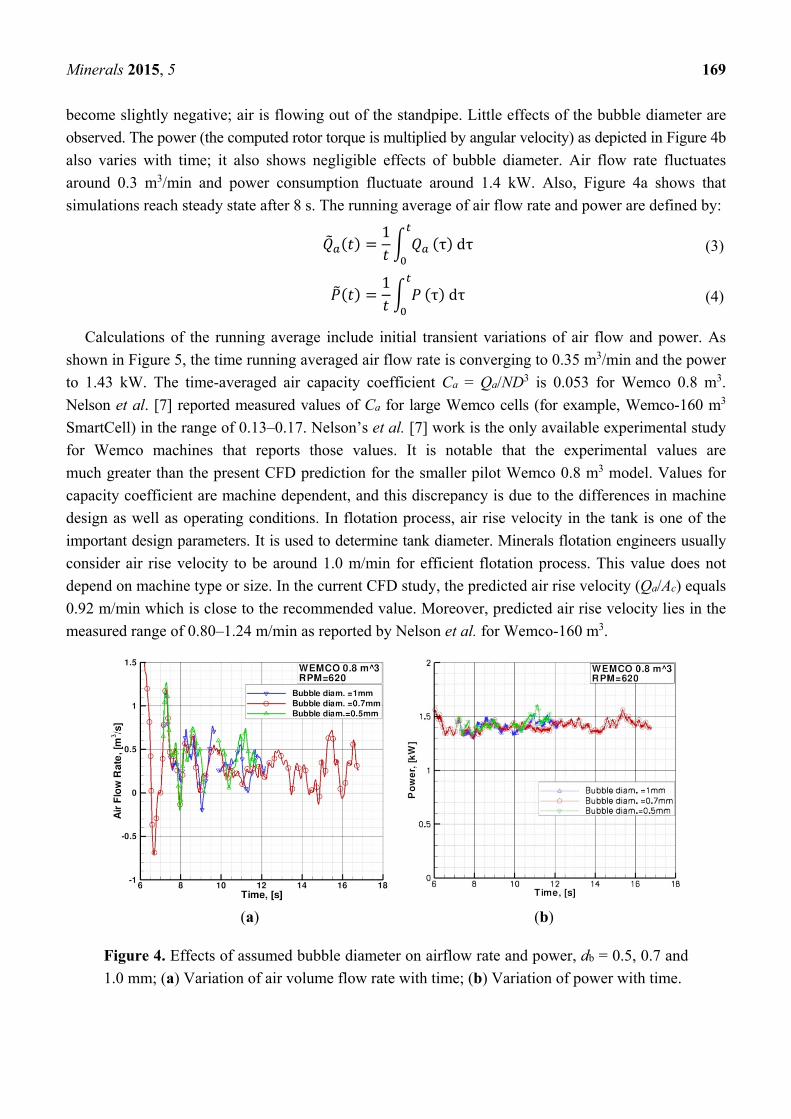
Minerals 2015, 5 169
become slightly negative; air is flowing out of the standpipe. Little effects of the bubble diameter are
observed. The power (the computed rotor torque is multiplied by angular velocity) as depicted in Figure 4b
also varies with time; it also shows negligible effects of bubble diameter. Air flow rate fluctuates
around 0.3 m3/min and power consumption fluctuate around 1.4 kW. Also, Figure 4a shows that
simulations reach steady state after 8 s. The running average of air flow rate and power are defined by: ( ) = 1 (τ) dτ (3)
( ) = 1 (τ) dτ (4)
Calculations of the running average include initial transient variations of air flow and power. As
shown in Figure 5, the time running averaged air flow rate is converging to 0.35 m3/min and the power
to 1.43 kW. The time-averaged air capacity coefficient Ca = Qa/ND3 is 0.053 for Wemco 0.8 m3.
Nelson et al. [7] reported measured values of Ca for large Wemco cells (for example, Wemco-160 m3
SmartCell) in the range of 0.13–0.17. Nelson’s et al. [7] work is the only available experimental study
for Wemco machines that reports those values. It is notable that the experimental values are
much greater than the present CFD prediction for the smaller pilot Wemco 0.8 m3 model. Values for
capacity coefficient are machine dependent, and this discrepancy is due to the differences in machine
design as well as operating conditions. In flotation process, air rise velocity in the tank is one of the
important design parameters. It is used to determine tank diameter. Minerals flotation engineers usually
consider air rise velocity to be around 1.0 m/min for efficient flotation process. This value does not
depend on machine type or size. In the current CFD study, the predicted air rise velocity (Qa/Ac) equals
0.92 m/min which is close to the recommended value. Moreover, predicted air rise velocity lies in the
measured range of 0.80–1.24 m/min as reported by Nelson et al. for Wemco-160 m3.
(a) (b)
Figure 4. Effects of assumed bubble diameter on airflow rate and power, db = 0.5, 0.7 and
1.0 mm; (a) Variation of air volume flow rate with time; (b) Variation of power with time.

Minerals 2015, 5 170
Figure 5. Running average of air flow rate and power.
4.2. Flow Pattern and Velocity Field.
The flow pattern in the Wemco rotor is very complex and unsteady. Analysis of the velocity field
and air volume fraction in the rotor region will shed light on the principle of the Wemco machine
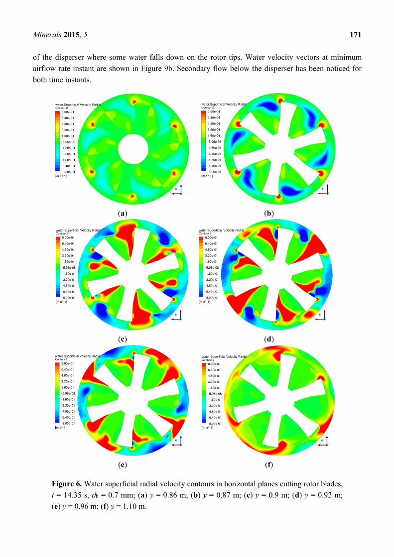
operation. Water superficial radial velocity contours on horizontal planes that cut the rotor are depicted
in Figure 6a–f at time t = 14.35 s. In Figure 6c, we see that the two blades at positions twelve-o’clock
and six-o’clock have the strongest radial outflow, whereas the two blades in the positions four-o’clock
and ten-o’clock have inward radial flow. The radial inward flow is entrained by the rotor from the
secondary flow below the disperser. The pumping situation switches at higher elevations as shown in
Figure 6e. Here, the radial flow at the blades at twelve-o’clock and six-o’clock is blocked whereas
that at the blades at four-o’clock and ten-o’clock is strong and outward. Hence, water exits the rotor
non-uniformly both circumferentially and vertically. Lack of flow periodicity in the Wemco rotor has
also been predicted by CFD simulations of single-phase flow in Wemco 250 and 300 conducted by the
present authors.
The velocity contours in the same planes are shown in Figure 7a–f at t = 15.4 s. At this instant, the
maximum airflow has been observed and the water content in the rotor is a maximum. The important
qualitative difference in the flow at this instant of time and the earlier one is the change in the direction
of the vertical velocity at the rotor top. Water flows from the rotor into the standpipe mainly through
the gap between rotor and disperser, and then falls down back from the standpipe mixed with air on
rotor blades. Then rotor blades pump this mixture through the upper row of disperser holes to the tank.
Figure 8a,b show the air volume fraction in a vertical mid plane that passes through the axis of the
machine at two different times where the airflow rate is minimum and maximum, respectively. A vortex
is formed in the standpipe, and water adheres to the standpipe walls under the effects of centrifugal forces
(i.e., water flows up into the standpipe with high circumferential velocity component). Consequently,
water head in the standpipe increases continuously until it reaches its maximum level. At this instant,
water breaks away from the standpipe walls and falls under gravity to the rotor tips capturing air with
it as a mixture as depicted in Figure 8a,b. Water velocity vectors in a mid-plane that passes through the
axis of the machine at two different time levels are shown in Figure 9a,b. Figure 9a shows the water
velocity vectors at the maximum airflow instant. Water is discharged radially through the upper holes
Minerals 2015, 5 171
of the disperser where some water falls down on the rotor tips. Water velocity vectors at minimum
airflow rate instant are shown in Figure 9b. Secondary flow below the disperser has been noticed for
both time instants.
(a) (b)
(c) (d)
(e) (f)
Figure 6. Water superficial radial velocity contours in horizontal planes cutting rotor blades,
t = 14.35 s, db = 0.7 mm; (a) y = 0.86 m; (b) y = 0.87 m; (c) y = 0.9 m; (d) y = 0.92 m;
(e) y = 0.96 m; (f) y = 1.10 m.

Minerals 2015, 5 172
(a) (b)
(c) (d)
(e) (f)
Figure 7. Water superficial radial velocity contours in horizontal planes cutting rotor blades,
t = 15.4 s, db = 0.7 mm; (a) y = 0.86 m; (b) y = 0.87 m; (c) y = 0.9 m; (d) y = 0.92 m;
(e) y = 0.96 m; (f) y = 1.10 m.

Minerals 2015, 5 173
(a) (b)
(c) (d)
(e) (f)
Figure 8. Air volume fraction and velocity contours for, db = 0.7 mm (a) air volume fraction,
t = 14.35 s; (b) air volume fraction, t = 15.4 s; (c) water superficial vertical velocity,
t = 14.35 s; (d) water superficial vertical velocity, t = 15.4 s; (e) water superficial radial
velocity, t = 14.35 s; (f) water superficial radial velocity, t = 15.4 s.

Minerals 2015, 5 174
(a) (b)
Figure 9. (a) Water superficial velocity vectors at maximum rate of air flow, db = 0.7 mm;
(b) water superficial velocity vectors at minimum rate of air flow, db = 0.7 mm.
Three uniform bubble diameters of 0.5, 0.7, and 1.0 mm have been used to study the effects of bubble
size on air holdup. Air holdup is computed by integration of (local) air void fraction over the pulp
volume and then divided by pulp volume. The computed air holdup for 0.5, 0.7, and 1.0 mm bubble
diameters are 9.3%, 7.4%, and 5.7%, respectively. It is observed that air holdup increases as bubbles
size decrease. In this study, drag and buoyancy are the only considered interfacial forces between air
bubbles and the liquid phase. Drag on air bubbles depends on bubble cross sectional area (i.e., db2)
while buoyancy depends on the bubble volume (i.e., db3). Therefore, drag is the dominant force for
small bubbles while buoyancy is the dominant force for large bubbles. Small bubbles have negligible
effective inertia and experience lower slip velocity to the liquid phase. They tend to penetrate deeper into
the tank and take longer time (i.e., retention time) to escape out at the free surface of the pulp, which
results in higher air holdup. Large bubbles experience higher slip velocity and escape quickly from the
tank because of the larger buoyancy that results in lower air holdup.
5. CFD-Based Flotation Model
Collisions rate between particles and bubbles is a critical factor for minerals recovery by flotation
machines. Collisions rate depends on the local turbulent dissipation rate in the pulp phase. Other factors
such as attachment and detachment rate of particles-bubbles aggregates depend on turbulent dissipation
rate as well as surface chemistry of particles and bubbles. Two-phase flow simulations of flotation
machines provide spatial distribution of air void fraction and turbulent dissipation rate. A CFD-based
flotation model has been developed in this work to predict pulp rate constant of Wemco 0.8 m3 pilot
cell. The model provides local values of collisions rate between particles and bubbles as well as
probabilities of attachment, collisions and stabilization. Abrahamson collision [8] model is commonly
used in estimation for collisions rate in flotation modeling. This paper provides an alternative more
accurate model for collisions rate developed by Zaichik et al. [9]. In this paper, we present flotation
model as a first rate equation. The rate constant in this equation depends on the local collisions frequency,
probability of collision, probability of attachment, and probability of stabilization.
Minerals 2015, 5 175
Yoon and Lutrell [10], Pyke et al. [11], Bloom and Heindel [12] among others developed theoretical
flotation models to predict pulp recovery rate. In these models, flotation process is represented
mathematically by a first order kinetic ODE Ordinary Differential Equation). These theoretical models
depend on the average air void fraction and dissipation rate for a given flotation cell. However,
distributions of turbulent dissipation rates and air volume fraction are not uniform and depend on the
design of the machine. Distribution of turbulent dissipation rate is the key factor in computing
recovery rate. Koh and Schwarz [13] developed a 3D CFD flotation model for a forced air Rushton’s
impeller flotation tank. Collisions frequency and flotation probabilities have been computed locally.
CFD simulations of flotation machines provide the spatial distribution of the rate of turbulent kinetic
energy dissipation and air void fraction throughout the cell. Flotation model is based on estimating
local recovery rate. Local recovery rate is the multiplication of collision kernel and probabilities of
collision, attachment and stabilization. These parameters depend mainly on dissipation rate throughout
the machine in addition to particles and bubbles sizes, surface tension and contact angle. The model
has been applied to a self-aerated flotation machine (Wemco 0.8) to predict pulp recovery rate. In this
paper, a range of particle sizes (10 μm ≤ dp ≤ 500 μm) have been used with three different bubble sizes
db = 0.5 mm, db = 0.7 mm, db = 1.0 mm to investigate the effects of particles and bubbles sizes on pulp
rate constant. Effects of feed particles size distribution has been studied also in this work.
5.1. Flotation Model: First-Order Rate Equation
The objective of a flotation model is to predict the recovery rate (rate of mass flow of useful minerals
collected from a flotation cell). Following Koh and Schwarz [13], we model the flotation kinetics as
a first-order rate process, which is given by the fundamental equation: = − + (5)
where is the particle number concentration (number of particles per unit volume) of free particles
(not attached to bubbles), is the number concentration of bubbles available for attachment (not
fully loaded bubbles), is the number of particle-bubble aggregates (bubbles that cannot accept
more particles but can lose particles), is the average particle-bubble attachment rate constant, and is the average particle-bubble detachment rate constant. We note the difference in the dimensions
(units) of (m3/s) and (1/s). The total particle number concentration is: = + (6)
where is the number concentration of particles attached to bubbles. All number concentrations are
functions of time and location in a flotation cell. A bubble is either fully loaded (cannot accept more
particles) or clean (no particles attached). The number of particle-bubble aggregates is proportional to
the total number of bubbles, = (7)
where is an average loading parameter, which varies with time and position. The number of clean
bubbles (those available for attachment) is = (1 − ) (8)

Minerals 2015, 5 176
The rate equation can now be written as: = − (1 − ) + (9)
The number of particles (S) that can be attached to a bubble is given by the ratio of surface area of
the bubble to the projected area of the particle. = 4 (10)
Such an estimation is not realistic. In Koh and Schwarz [13] work, only half of that number is
assumed as a first approximation. = 0.5 = 2 = β (11)
Rearranging, we obtain: = = 2 (12)
5.2. Attachment Model
Collisions frequency (Z ) of two groups of dispersed species (e.g., particles and bubbles) is the
number of collisions per unit volume per unit time (m−3·s−1). It is proportional to the product of the number densities Nb and Np of bubbles and particles (Z = β ), where β is called the collisions
kernel (m /s). The attachment rate constant ( , m /s) is defined as the product of particle-bubble
collisions kernel times probabilities (or efficiencies). This is because not every collision event leads to
successful attachment of a particle to a bubble. Following Koh and Schwarz [13], the attachment rate
constant is written as: = β (13)
where Pc, Pa, and Ps are probabilities of particle-bubble collision, adhesion, and stabilization.
Multiplication by Pc is questionable since it should be considered as a part of the collisions kernel.
Apparently including Pc is a remnant of the original model that was developed under quiescent
conditions. This collisions probability Pc should be eliminated because collisions kernel is modeled
under turbulent conditions, and the assumption of laminar flow is irrelevant. When turbulence is
the mechanism of collisions of particles and bubbles, “quiescent” conditions should be defined as
the turbulent fluctuations ′ and turbulent dissipation rate that maximizes the attachment rate and
minimizes detachment.
5.3. Collision Kernel
The collision kernel β is perhaps the most important ingredient of the attachment rate constant .
For turbulent flows, two classical models are in use. The first is Saffman and Turner model [14], which
is applicable in the limit of zero Stokes particle number. The second is Abrahamson model [8] which is

Minerals 2015, 5 177
applicable in the limit of infinite particle Stokes number. The form of the later model is usually written
(Schubert and Bischofberger 1979) [15] as: β = 5 +2 + (14)
where and are the turbulent ( ) fluctuating velocities of the particles and bubbles relative to
the carrier liquid, respectively. Leipe and Mockel’s [16] formula (not the original formula by
Abrahamson) is used for these velocities,
= 0.4 ϵ / // ρ − ρρ / (15)
where ϵ is dissipation rate of the turbulent kinetic energy per unit mass (w/kg), and ρ are the
kinematic viscosity and density of the liquid, respectively. ρ and d are the density and diameter of
the colliding particles, = for particles and = for bubbles. The mass density for a bubble is assumed to be equal 0.5ρ , as if the bubble mass is the virtual mass of a spherical bubble. This equation
implies that high dissipation results in higher collisions rates between bubbles and particles, and in this
regard high dissipation has favorable effects on flotation. Schubert [15] model have been developed
for very high inertia particles. In minerals, flotation particles have a wide spectrum of inertia.
Therefore, application of Schubert collisions model results in over prediction of collision kernel as
discussed by Fayed [17].
Zaichik et al. [9] developed another statistical model for the collisions kernel for particles and
bubbles. The model applies to arbitrary values of density ratio and particle sizes. This model has been
validated by Fayed and Ragab [18] to study its limitation and it provides more accurate prediction for
collisions kernel than Schubert model [15]. The model is not presented here because of the space and
interested reader is referred to Zaichik et al. [9] and Fayed [17] where the model has been presented
and discussed extensively. In this paper, comparison between Schubert model [15] and Zaichik et al.
model [9] is presented to show the over-estimation of collision kernel by the former model. Hence,
Zaichik et al. model [9] has been used herein for more accurate prediction of collision kernel.
5.4. Flotation Probabilities
Process of minerals flotation involves two main events which are collisions of particles with
bubbles and attachment of the colliding particles with bubbles. The first event happens under turbulent
flow conditions where particles and bubbles sizes and turbulent velocity rms fluctuations are the main
variables that control this event. Upon collision, useful minerals particles have to attach to the bubble
and then transported to the froth phase by buoyancy of bubbles. The attachment process is due to the
adhesive forces between particles and bubbles and then stabilization of the particle-bubble aggregates.
An accurate model for collisions frequency of particles and bubbles has been used in this work [9] to
estimate kernel collisions. The second step is to model for the probability of particles’ attachment to a
bubble. In the literature, considerable efforts have been made to model for the probabilities of
collisions, adhesion and stabilization. The concept of probability of collisions has been developed
under laminar flow conditions which do not exist in minerals flotation. In this section, we summarize
and present models for probabilities of collisions, adhesion and stabilization developed by other

Minerals 2015, 5 178
authors. These models have been used in our CFD-flotation model to predict pulp recovery rate of a
flotation cell. Hopefully, some validation work will be completed on a fundamental level in future to
study the limitations of these models and their accuracy.
The probability (efficiency) of collision Pc is given by a formula due to Yoon and Luttrell [10], = 32 + 415 . dd (16)
where the bubble Reynolds number is defined by = . In the actual calculations is limited
to a maximum of 1.
The expression for probability of adhesion Pa is also derived by Yoon and Luttrell [10],
= sin 2 tan exp − 45 + 8 .15 d dd + 1 (17)
where is the induction time, which is determined by an empirical formula due to Dai et al. [19]: = 75θd . (18)
where is measured in seconds, θ is particle-bubble contact angle in degrees, and is the particle
diameter in meters.
The formula proposed by Schulze [20] and modified by Bloom and Heindel [12] for the probability
of stabilization is used: = 1 − exp 1 − 1min(1, Bo∗) (19)
where the modified Bond number is defined by:
Bo∗ = d Δρg + 1.9ρ ϵ (d2 + d2 ) + 1.5 d 4 σd − d ρg sin (π− θ2)6 σ sin π − θ2 sin π + θ2 (20)
where As = 0.5 is an empirical constant suggested by Bloom and Heindel [12], where σ is the surface tension (N/m), Δρ = ρ − ρ , and g is the gravitational acceleration.
5.5. Detachment Model
The particle-bubble detachment rate constant ( ) is defined by: = = Z (1 − ) (21)
The probability of detachment is assumed to be equal to (1 − ). Koh and Schwarz [13] justified
the inclusion of in both and because the processes involve different turbulent eddies acting
independently of each other. The detachment frequency is given by Bloom and Heindel [12] as:
= C εd + d (22)

Minerals 2015, 5 179
where = 2.0 is an the empirical constant. We note in this equation the unfavorable effects of
dissipation that high dissipation results in destabilization of particle-bubble aggregates.
5.6. Particle Size Distribution
Particles in the feed slurry to a flotation machine have a particle size distribution. Several models in
the literature have been developed to account for different particles properties in the feed slurry. These
models predict the global rate constant of a flotation cell and classified into three groups—discrete rate
constant distribution, continuous rate constant distribution and mean rate constant. Several discrete rate
constant models have been developed but they differ in the number of fractions (Morris [21], Kelsall [22],
Cutting [23], Jowett [24], Imaizumi [25]). Two fraction discrete models developed by (Kelsall [22])
are named as fast float and slow float fractions. Continuous rate constant models assume that rate
constants are distributed as a continuous distribution represented by a Gamma-distribution function
(Harris [26], Woodburn [27], Loveday [28], Kappur [29]). The mean rate constant model has been
proposed by Chen (Chen Z.M. [30,31]). However, prediction of rate constant in all flotation models is
strongly affected by operating conditions as well as particles and bubbles properties on a local basis.
Flotation modeling using CFD enables more accurate prediction of rate constant and helps to assess the
performance of a flotation cell.
The attachment rate as given above is mainly a function of bubble size, particle size, air/water
surface tension and contact angle. An effective pulp recovery rate constant proposed here is
defined by: ∗ = α (1 − α) (23)
We recognize the factor as the local number concentration of bubbles, and the factor (1 − α) is
included so that in a region of high air volume fraction (α ≈ 1)the recovery rate should drop to zero. The local number concentration of particles depends on slurry loading, and we expect it to be
proportional to the local water volume fraction, (1 − α). We believe that including the factor (1 − α)
gives a better figure of merit that can be used to evaluate different designs in the absence of distribution. The machine average rate constant is obtained by integration over the machine volume,
∗ = ∗ (1 − ) (24)
where is a froth recovery factor.
Minerals particles in the feed slurry have a size distribution and this distribution has great impact on
recovery rate. Let ( ) denote the pdf of particle size distribution. Particle size distribution depends
on the grinding process and metallurgical properties of the minerals particles. The current CFD-based
flotation kinetic model can be used to determine pulp recovery rate for both bubble size and particle
size distributions. We assume a Gamma-distribution for the particles number density function. = −Γ( ) exp − −
(25)
Minerals 2015, 5 180
where μ is the minimum possible particle diameter and Γ is the Gamma function. In this paper, we
used μ = 0 and = 30. To obtain different particles number distributions, we assign different
values for γ starting from 1.0–15, incremented by one. This also changes the mean diameter. The
pseudo rate constant for particle size distribution ∗is computed:
∗ = (λ) ∗(λ),, λ (26)
and , , , are the minimum and maximum particle diameters present in the feed slurry.
5.7. Flotation Results
In this section, we demonstrate the viability of CFD-based flotation model as a tool to evaluate the
performance of flotation machines and provide detailed hydrodynamic and kinetics data that can help
improve the design of such machines. Ragab and Fayed [32] developed a CFD-based flotation model,
and used it to determine the effects of particle size on the rate constant. We use particle specific gravity ρ = 4.1, contact angle θ = 40°, and surface tension σ = 0.06 / as input parameters to the flotation
model. Two-phase hydrodynamic simulations provided spatial distributions of dissipation rate, ϵ, and
air volume fraction, α(also called void fraction). The number concentration of bubbles is = α/ ,
where is the bubble volume and spherical bubbles are assumed. Particles-bubbles collisions rate has
been estimated using Zaichik et al.’s model [9]. Zaichik et al.’s model and probabilities models rely on
velocity fluctuations, bubble diameter, particle diameter, particle density, air void fraction, contact
angle and air-water surface tension coefficient. Velocity fluctuation, ′ has been estimated from the
local eddy viscosity and dissipation rate. Local air void fraction is obtained from the CFD results of
the two-phase flow. Other parameters are user input. CFD-based flotation kinetics model is a post
processing program to the two-phase simulations runs of flotation cells such as Wemco 0.8 m3. Effects
of particles size distribution on pulp recovery rate are presented here.
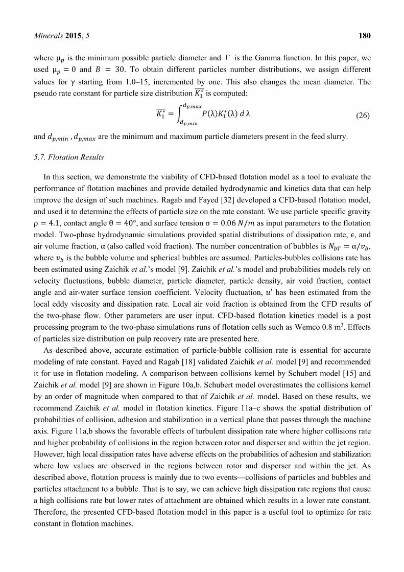
As described above, accurate estimation of particle-bubble collision rate is essential for accurate
modeling of rate constant. Fayed and Ragab [18] validated Zaichik et al. model [9] and recommended
it for use in flotation modeling. A comparison between collisions kernel by Schubert model [15] and
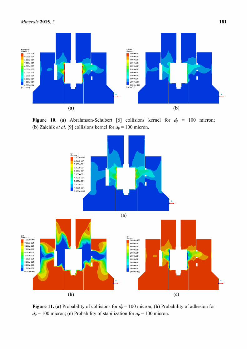
Zaichik et al. model [9] are shown in Figure 10a,b. Schubert model overestimates the collisions kernel
by an order of magnitude when compared to that of Zaichik et al. model. Based on these results, we
recommend Zaichik et al. model in flotation kinetics. Figure 11a–c shows the spatial distribution of
probabilities of collision, adhesion and stabilization in a vertical plane that passes through the machine
axis. Figure 11a,b shows the favorable effects of turbulent dissipation rate where higher collisions rate
and higher probability of collisions in the region between rotor and disperser and within the jet region.
However, high local dissipation rates have adverse effects on the probabilities of adhesion and stabilization
where low values are observed in the regions between rotor and disperser and within the jet. As
described above, flotation process is mainly due to two events—collisions of particles and bubbles and
particles attachment to a bubble. That is to say, we can achieve high dissipation rate regions that cause
a high collisions rate but lower rates of attachment are obtained which results in a lower rate constant.
Therefore, the presented CFD-based flotation model in this paper is a useful tool to optimize for rate
constant in flotation machines.
Minerals 2015, 5 181
(a) (b)
Figure 10. (a) Abrahmson-Schubert [6] collisions kernel for dp = 100 micron;
(b) Zaichik et al. [9] collisions kernel for dp = 100 micron.
(a)
(b) (c)
Figure 11. (a) Probability of collisions for dp = 100 micron; (b) Probability of adhesion for
dp = 100 micron; (c) Probability of stabilization for dp = 100 micron.

Minerals 2015, 5 182
The product of collision kernel and probabilities of collision, adhesion and stabilization gives the
local attachment rate . An effective pulp recovery rate constant (in the absence of detachment) is
defined here by α(1 − α)/ , and corresponding contours are depicted in Figure 12a–d. The factor (1 − α) is included in this definition so that in a region of 100% air (α = 1.0) the local recovery rate
should be zero. The spatial distribution of α(1 − α), which is zero if α = 0.0 or α = 1.0 and maximum
if α = 0.5 (50% void fraction), implies that the local recovery rate is maximized when the air is well
dispersed throughout the machine. The actual recovery rate will depend on the balance between the
favorable effects of dissipation rate ϵ in increasing the collision frequency against its adverse effects on
reducing the attachment rate and increasing detachment rate. Therefore, knowing the spatial
distributions of both α and ϵ throughout the machine is essential in understanding the effectiveness of
different components (rotor, stator or disperser, jets) on the flotation efficiency. Only through CFD of
two-phase simulations (or elaborate experimental measurements) one can determine those spatial
distributions. This is a clear advantage of CFD-based flotation models in comparison with models that
treat the entire cell as one unit which assumes a single value for determined by the consumed power
and single value for α that is equal to the gas holdup.
(a) (b)
(c) (d)
Figure 12. (a) Pulp recovery rate ∗ for 40 μm particle diameter; (b) Pulp recovery rate ∗ for 100 μm particle diameter; (c) Pulp recovery rate ∗ for 200 μm particle diameter; (d) Pulp
recovery rate ∗ for 300 μm particle diameter.

Minerals 2015, 5 183
Particle diameter has significant effects on distribution of the pulp rate constant ∗ throughout
the Wemco machine. Contours of ∗ in a vertical mid plane are shown in Figure 12a–d, for particle diameters of 40, 100, 200, and 300 μm. Fine particles < 50μm are efficiently recovered
in the high dissipation region between the rotor and disperser. For a medium particle diameter of 100μm ≤ ≤ 200μm, recovery happens in the jets out of the disperser. For coarse particles ≥ 300μm pulp recovery is more efficient in the moderate dissipation regions outside the disperser
below, above and between the disperser jets. In the present work, the pseudo rate constant is computed
as a function of particle diameter for two values of contact angle (θ = 40° and θ = 50°). Values for
rate constant are obtained for different uniform bubble size and different uniform particle size. Average flotation rate constant ∗can be defined according to the Equation (24) where is a froth
recovery factor. We assumed = 1.0 and β = 0.0 for a fully unloaded bubble and studied the effects
of bubble diameter, particle diameter, and contact angle on ∗. The results are shown in Figure 13a–c.
As expected, rate constant increases with the increase of contact angle. Also, higher rate constant is
observed for smaller bubble size ( = 0.5mm) because air holdup increases for smaller bubble
diameter, and hence higher bubble concentration number, as well as a lower rate constant for larger
bubble diameter due to the decreases in the air holdup (i.e., local bubbles number concentration). The
maximum recovery rate shifts to higher particle diameter with the increase in bubble diameter. The
recovery rate shown in these figures is very high relative to experimental data reported in literature because of the assumed values of and β. Maximum rate constant for bubble sizes of 0.5, 0.7 and 1.0
mm occur at particle size of 125, 150 and 175 μm, respectively. This reveals that fact that smaller
bubbles sizes (db < 0.5 mm) are needed to float very tiny particles (dp < 100 μm).
Next, we study the effects of particles size distribution on the mean flotation rate constant. As
shown in Figures 13a–c, rate constant is dramatically affected by particle sizes and the feed slurry to a
flotation cell contains a wide spectrum of particles sizes. Therefore, modeling for rate constant with
particle size distribution is more realistic and useful. Samples of assumed particles’ number
distribution are shown in Figure 14 for B = 30 and three different values for γ (γ = 2, 3 and 5).
Changing values for γ changes the size distribution and mean diameter of the particles. In real samples,
this distribution depends on the grinding process as well as metallurgical properties of the ore. The
procedure herein is to apply the present CFD flotation model for a single particle size and uniform
bubble diameter in the postprocessor of the used CFD package (CFX). Using Equation (23), we obtain
the local rate constant for a specific particle size. We used particles sizes ranging from 10–500 μm to
be within the practical particle sizes. We used Equation (24) to obtain the average rate constant over
the pulp volume and from Equation (26) we calculate the average pulp rate constant for a specific
distribution. This process yields a single value for the rate constant that we attribute to the mean value
of the proposed particle size. Different particle number distributions pdfs are used (each has different
mean diameter) to plot rate constant versus particles mean diameter. This deterministic method in the
calculation of rate constant for certain particle size distribution is more robust than the other probabilistic
models [26–29]. This is because the effects of all variables such as surface tension, contact angle,
bubbles size and particles size are explicitly included in the model.

Minerals 2015, 5 184
(a)
(b) (c)
Figure 13. (a) Average rate constant for 0.5 mm bubble diameter and for single particle
sizes; (b) average rate constant for 0.7 mm bubble diameter and for single particle sizes;
(c) average rate constant for 1.0 mm bubble diameter and for single particle sizes.
Figure 14. Assumed particles number distribution, B = 30.

Minerals 2015, 5 185
The effect of particles size distribution on the rate constant has been studied also by an assumed
γ-particle number distribution. Effects of different size distribution on mean rate constant are depicted
in Figure 15a–c for different bubbles sizes. Figure 15a shows that the maximum rate constant is around
the mean particle diameter of 140 μm for a contact angle of 50°, and the particle diameter of 120 μm
for a contact angle of 40° where, increasing contact angle increases the possibilities of floating larger
particles. A considerable mean rate constant for very small mean diameter (dmean = 5 μm) is observed
for bubble size of 0.5 mm while very low rate constant exists for the larger bubble size (dmean = 0.7 and
1.0 mm) at the same particle mean diameter. Maximum mean rate constant for bubble size (dmean = 0.7
mm) is also observed to be around particle mean diameter 140 and 180 μm for bubble size (dmean = 1.0
mm) as shown in Figure 15b,c.
(a)
(b) (c)
Figure 15. (a) Average rate constant for 0.5 mm bubble diameter and for particle
no. γ-distribution; (b) average rate constant for 0.7 mm bubble diameter and for particle
no. γ-distribution; (c) average rate constant for 1.0 mm bubble and diameter for particle
no. γ-distribution.

Minerals 2015, 5 186
6. Conclusions
Two phase simulations of self-aerated flotation Wemco 0.8 m3 pilot cells have been conducted to
study the transient flow structures and predict air flow rate and power consumption as a function of
time. The newly devised overflow tank on top of the pulp volume and constant static pressure at the
top boundary of this tank and the standpipe opening allowed us to predict the airflow rate and the
transient position of the pulp–air interface until it reached a steady position. Also, investigating
dynamical behavior of two-phase flow in the standpipe provides us with a detailed picture of the
mixing of air and water and pumping this mixture into the tank. The two-phase simulations provide us
with essential parameters for flotation modeling such as local turbulent dissipation rate, velocity rms
fluctuations and air void fraction throughout the whole machine. These parameters have been used to
develop a CFD-based flotation model. This model predicts pulp rate constant for an arbitrary particle
size and bubble size. It uses a first-order rate equation, where processes of collision, attachment and
detachments are described by well-known theoretical and empirical formulae. The model uses local
values of the rate of turbulent energy dissipation and air volume fraction. Not only the average pulp
recovery rate can be estimated but also the regions of high/low recovery rate can be identified. The
CFD-based flotation model presented here is also used to determine the dependence of recovery rate
constant at any locality within the pulp on bubble diameter, particle diameter, particle specific gravity,
contact angle, and surface tension. Furthermore, we have updated our CFD-based flotation kinetics
model to predict pulp recovery rate in the presence of both particles size distributions. The calculations
are repeated for many particle diameters selected from a range that covers the anticipated minimum
and maximum diameters in the slurry. The particles number density pdf and the data generated for
single particle size are used to compute the recovery rate for a specific mean particle diameter. Our
computational model gives a figure of merit for the recovery rate of a flotation machine, and as such
can be used to assess incremental design improvements and design of new machines. The model is a
very useful design tool because it can be used to establish the effects of different components (rotor,
stator, or disperser jets) on the pulp recovery.
Acknowledgment
This work has been supported by FLSmidth Minerals Inc., Salt Lake City, Utah.
Author Contributions
Dr. Fayed and Dr. Ragab worked closely on the material presented in this paper during the time
Dr. Fayed was working as Graduate Research Assistant in Department of Engineering Science and
Mechanics, Virginia Tech, USA. Dr. Fayed constructed geometric models of Wemco machine,
generated the mesh, and conducted computer simulations. Dr. Ragab contributed to the
theoretical modeling and boundary conditions. Both authors contributed equally to data analysis and
drawing conclusions.
Conflicts of Interest
The authors declare no conflict of interest.

Minerals 2015, 5 187
References
1. Koh, P.T.L.; Schwarz, P. CFD Model of a Self-Aerating Flotation Cell. Int. J. Miner. Process.
2007, 85, 16–24.
2. Tiitinen, J.; Koskinen, K.; Ronkainen, S. Numerical modeling of an Outokumpu flotation cell.
In Proceedings of the Centenary of Flotation Symposium, Brisbane, Australia, 6–9 June 2005.
3. Kerdouss, F.; Bannari, A.; Proulx, P. CFD modeling of gas dispersion and bubble size in a double
turbine stirred tank. Chem. Eng. Sci. 2006, 61, 3313–3322.
4. Prosperetti, A.; Tryggvason, G. Computational Methods for Multiphase Flow; Cambridge University
Press: Cambridge, UK, 2007.
5. Clift, R.; Grace, J.R.; Weber, M.E. Bubbles, Drops and Particles; Dover Publications: Mineola,
NY, USA, 2005.
6. Van den Akker, H.E.A. Toward a truly multiscale computational strategy for simulating turbulent
two-phase flow processes. Ind. Eng. Chem. Res. 2010, 49, 10780–10797.
7. Nelson, M.; Traczyk, F.; Lelinski, D. Design of Mechanical Flotation Machines. In Proceedings
of the 2011 SME Annual Meeting, Denver, Colorado, USA, 27 February–2 March 2011.
8. Abrahamson, J. Collision rate of small particles in a vigorously turbulent fluid. Chem. Eng. Sci.
1975, 30, 1371–1379.
9. Zaichik, L.I.; Simonin, O.; Alipchenkov, V.M. Turbulent collision rates of arbitrary density
particles. Int. J. Heat Mass Transf. 2010, 53, 1613–1620.
10. Yoon, R.H.; Luttrell, G.H. The effect of bubble size on fine particle flotation. Miner. Process.
Extr. Metall. Rev. 1989, 5, 101–122.
11. Pyke, B.; Fornasiero, D.; Ralston, J. Bubble particle heterocoagulation under turbulent conditions.
J. Colloid Interface Sci. 2003, 265, 141–151.
12. Bloom, F.; Heindel, T.J. Modeling flotation separation in semi-batch process. Chem. Eng. Sci.
2003, 58, 403–422.
13. Koh, P.T.L.; Schwarz, M.P. CFD modeling of bubble-particle attachments in flotation cells.
Miner. Eng. 2006, 19, 619–626.
14. Saffman, P.G.; Turner, T.S. On the collision of drops in turbulent clouds. J. Fluid Mech. 1956, 1,
16–30.
15. Schubert, H. On the turbulence-controlled microprocesses in otation machines. Int. J. Miner.
Process. 1999, 56, 257–276.
16. Leipe, F.; Mockel, O.H. Untersuchungen zum stoffvereinigen in ussiger phase. Chem. Technol.
1976, 30, 205–209. (In German)
17. Fayed, H. Particles and Bubbles Collisions in Homogeneous Isotropic Turbulence and
Applications to Minerals Flotation Machines. Ph.D. Thesis, Virginia Tech, Blacksburg, VA, USA,
6 December 2013.
18. Fayed, H.E.; Ragab, S.A. Direct Numerical Simulation of Particles-Bubbles Collisions Kernel in
Homogeneous Isotropic Turbulence. J. Comput. Multiph. Flows 2013, 5, 168–188.
19. Dai, Z.; Fornasier, D.; Ralston, J. Particle-bubble attachment in mineral flotation. J. Colloid Interface
Sci. 1999, 217, 70–76.

Minerals 2015, 5 188
20. Schulze, H.J. Flotation as a hetrocoagulation process: Possibilities of calculation the probability of
flotation. In Coagulation and Flocculation; Dobias, B., Ed.; Marcel Dekker: New York, NY,
USA, 1993; pp. 321–363.
21. Morris, T.M. Discussion of flotation rates and flotation efficiency. Min. Eng. 1952, 4, 794–798.
22. Kelsall, D.F.; Stewart, P.S. A critical review of applications of models of grinding and flotation.
In Proceedings of the Symposium on Automatic Control Systems in Mineral Processing Plant,
Brisbane, Australia, 17–20 May 1971; pp. 213–232.
23. Cutting, G.W.; Devenish, M.A. Steady-state model of froth flotation structures. In Proceedings of
the AIME Annual Meeting, New York, NY, USA, 20 February 1975.
24. Jowett, A. Resolution of flotation recovery curves by a difference plot method. Trans. IMM 1974, 70,
191–204.
25. Imaizumi, T.; Inoue, T. Kinetic considerations of froth flotation. In Proceedings of the 6th
International Mineral Processing Congress, Cannes, France, 26 May–2 June 1963; pp. 581–593.
26. Harris, C.C.; Chakravarti, A. Semi-batch froth flotation kinetics; species distribution analysis.
Trans. AIME 1970, 247, 162–172.
27. Woodburn, E.T.; Loveday, B.K. Effect of variable residence time data on the performance of
a flotation system. J. South Afr. Inst. Min. Metall. 1965, 65, 612–628.
28. Loveday, B.K. Analysis of froth flotation kinetics. Trans. IMM 1966, 75, 219–225.
29. Kapur, P.C.; Mehrotra, S.P. Estimation of the flotation rate distributions by numerical inversion of
the Laplace transform. Chern. Eng. Sci. 1974, 29, 411–415.
30. Chen, Z.M.; Wu, D.C. A study of flotation kinetics. Nonferr. Met. 1978, 10, 28–33.
31. Chen, Z.M.; Mular, L. A study of flotation kinetics—A kinetic model for continuous flotation.
Nonferr. Met. 1982, 3, 38–43.
32. Ragab, S.; Fayed, H. CFD-Based Flotation Model for Prediction of Pulp Recovery Rate.
In Proceedings of the SME Annual Meeting and Exhibit, Seattle, WA, USA, 19–22 February
2012.
© 2015 by the authors; licensee MDPI, Basel, Switzerland. This article is an open access article
distributed under the terms and conditions of the Creative Commons Attribution license
(http://creativecommons.org/licenses/by/4.0/).