Minimal Coordinates Formulation of Contact Dynamics

Abhinandan Jain1

1 Jet Propulsion Laboratory, California Institute of Technology, 4800 Oak Grove Drive, Pasadena, CA, 91109 USA,Abhi.Jain@jpl.nasa.gov

Abstract

In recent years, complementarity techniques have been developed for modeling non-smooth dynamics arising from con-tact and collision problems for multi-link robotic systems. The commonly used complementarity approach sets up a linearcomplementarity problem (LCP) using non-minimal coordinates together with all the unilateral contact constraints andinter-link hinge and loop closure bilateral constraints onthe system. In this paper, we develop a complementarity for-mulation that uses an operational space approach. It uses minimal coordinates resulting in a much smaller LCP problemwhose size is independent of the number of bodies and the number of degrees of freedom in the system. Furthermore,we exploit operational space low-order algorithms to overcome key computational bottlenecks to obtain over an order ofmagnitude speed up in the solution procedure.

Keywords: robotics, multibody dynamics, non-smooth dynamics

1 Introduction

For more than a decade, researchers have been developing complementarity based approaches for formulating and solvingthe equations of motion of systems with contact and collision dynamics [1–3]. Examples of such dynamics for roboticsystems include manipulation and grasping tasks such as illustrated in Figure 1, and legged locomotion. The complemen-tarity approach models bodies as rigid, and uses impulsive dynamics to handle non-smooth collision, contact interactionsand mode transitions. By impulsively “stepping” over non-smooth events, complementarity methods avoid small time stepsize and stiffening issues encountered with penalty based methods which allow surface compliance during contact [4].

Figure 1. An example multi-arm robot manipulation taskinvolving unmounting a wheel from a hub involving severalcontact and collision dynamics interaction events.

In this paper, we focus on the analytical and computational as-pects of a minimal coordinate formulation of the complemen-tarity approach to contact and collision dynamics for multi-linksystems. This paper further extends the operational space formu-lation for contact and collision dynamics described in reference[5]. We adopt the complementarity based physics models from[2, 3].

The complementarity based solution consists of a combina-tion of: (a) setting up alinear complementarity problem (LCP)problem; (b) numerically solving the LCP problem; and (c) an-cillary dynamics computations. The LCP depends on the linkmass and inertia properties, contact friction parameters,inter-link bilateral constraints and contact and collision unilateral con-straints. The LCP solution identifies the unilateral constraintsthat are active, and solves for the impulsive forces and velocitychanges that are consistent with the constraints on the system.Variants of the complementarity approach to handle elasticandinelastic collisions have also been developed [3]. While LCPfor-mulations use discretized approximations for the frictioncones,other researchers have explored non-linear cone complementar-ity approaches that avoid such approximations [6].

The typical approach to handling contact and collision dynamics is to work with non-minimal coordinates, since itis the easiest to set up [3]. In this formulation, the LCP stage does most of the work, but the LCP dimension is largeand computationally expensive to solve. For a multi-link system withn links, the standard LCP approach uses 6n non-minimal coordinates together with the bilateral constraints associated with the inter-link hinges and the unilateralcontact

ECCOMAS Multibody Dynamics 2013

1-4 July, 2013, University of Zagreb, Croatia

163

constraints. This approach has a mass matrix that is block diagonal and constant. Besides the large LCP problem size,this formulation requires additional techniques for managing error drift in the bilateral constraints when integrating theequations of motion.

An alternative approach is to use minimal hinge coordinatesthat automatically eliminate the bilateral constraintsfor the inter-link hinges [7]. While the underlying physics remains unchanged, this formulation reduces the size of theLCP problem, and avoids the need for managing bilateral constraint violation errors for the hinges. However, the use ofminimal coordinates leads to a dense and configuration dependent mass matrix. Thus while minimal coordinates lead tosmaller LCP problems, they also typically significantly increase the difficulty and computational complexity of setting upthe LCP problem. This has been a significant hurdle in the use of minimal coordinate approaches.

In this paper we explore a progression of minimal coordinateformulations that partition the overall solution effortin different ways between setting up the LCP problem, and solving it. Our goal is to reduce the overall computationalcomplexity by taking advantage of the smaller dimension of minimal coordinate models together with the host of structurebased, recursive and low-order dynamics algorithms that are available for articulated system dynamics. Notable exam-ples of such structure based algorithms include the composite rigid body algorithms for computing the mass matrix [8],the articulated body inertia forward dynamics algorithm [9] and the spatial operator based operational space dynamicsalgorithm [10].

The main contribution of this paper is in the development of an operational space basedOS formulation, that whileusing minimal coordinates for the contact and collision dynamics problem, uses low-order spatial operator algorithmstoovercome the complexitys of setting up the LCP problem. Thisresults in a more than an order of magnitude reduction incomputational complexity. The size of the resulting LCP problem is independent of the number of links and generalizedcoordinates, and only depends on the number of contact nodes. We also describe extensions of the formulation to handleelastic and inelastic collision dynamics. The different formulations are developed and described in a way so as to clarifythe relationships among them and methods available in the literature.

We use a multi-link pendulum numerical problem to quantitatively and parameterically measure the performanceimprovements from the new OS formulation. We have also applied the OS formulation to simulate manipulations tasksinvolving contact and collision interactions for a dual-arm robot system. This dual-arm robot is used as a reference systemto compare the LCP sizes for the different formulations discussed in this article.

The organization of this paper is as follows. Section 2 describes the complementarity conditions associated withmodeling a single unilateral contact constraint. In Section 3 we describe the system-level, multiple contactsNMC LCPformulation based on non-minimal coordinates that is widely used. While easy to set up, this formulation leads to a largeLCP problem. Section 4 discusses a similarMC formulation based on the use of minimal coordinates. We observe thatthe reduction in the size of the LCP is accompanied by an increase in the complexity of setting up the LCP. Section 5further transforms the MC LCP formulation to develop theRMC formulation that further reduces the size of the LCPproblem, but at the cost of an increase in the LCP setup complexity. Section 6 develops theOSformulation that is basedon an operational space approach. While the LCP size is moderately larger than from the RMC approach, it opens thepath to exploiting low-order operational space algorithmsto significantly reduce the LCP setup complexity. Section 7extends the OS formulation contact dynamics model to include elastic and inelastic collision dynamics. Section 8 focuseson computational issues, and describes operational space computational algorithms to reduce the complexity of settingup the OS LCP problem. The section also includes results froma numerical simulation to quantify the performanceimprovements for the OS formulation.

2 Unilateral contact constraints

Unilateral constraints are defined by inequality relationships of the form

d(θ, t) > 0 (1)

for some functiond of the configuration coordinatesθ and timet. As an example, the non-penetration condition forrigid bodies can be stated as an inequality relationship requiring that the distance between the surfaces of rigid bodies benon-negative.d(θ, t) is generally referred to as thedistanceor gapfunction.

Contact occurs at the constraint boundary, i.e., whend(θ, t) = 0. For bodies in contact, the surface normals atthe contact point are parallel. The existence of contact is typically determined using geometric or collision detectiontechniques. For a pair of bodiesA andB in contact, we use a convention where theith contact normaln(i) is definedas pointing from bodyB towards bodyA, so that motion ofA in the direction of the normal leads to a separation of thebodies. A unilateral constraint is said to be in anactivestate when

d(θ, t) = d(θ, t) = d(θ, t) = 0 (2)

164 A. Jain

Thus, a unilateral constraint is active when there is contact, and the contact persists. Only active constraints generateconstraint forces on the system. A constraint that is not active is said to beinactive. Contactseparationoccurs whenthe relative linear velocity of the contact points along thenormal becomes positive and the contact points drift apart.Aseparating constraint is in the process of losing contact and transitioning to an inactive state. At the start of a separationevent, we have

d(θ, t) = d(θ, t) = 0 and d(θ, t) > 0 (3)

2.1 Contact impulse for an active contact constraint

polyhedralapproximation

directionvectors

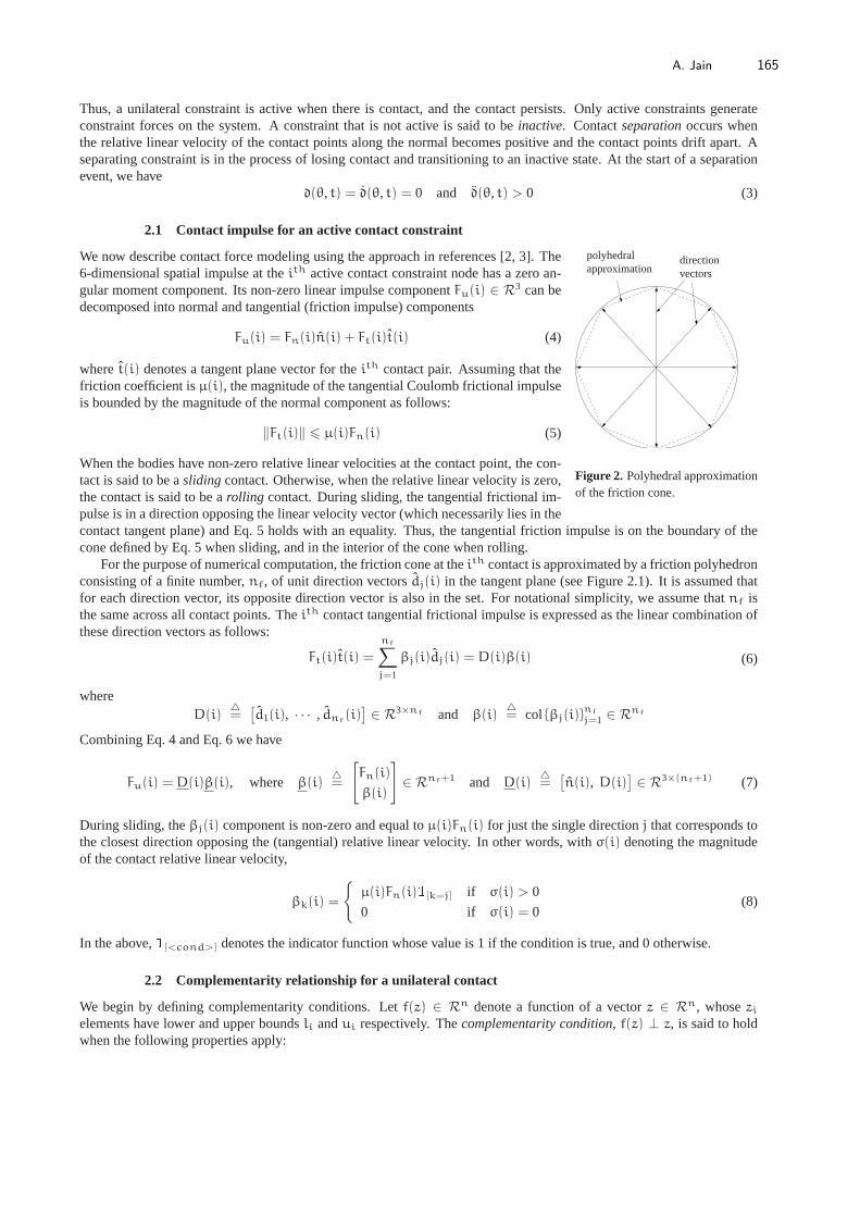
Figure 2. Polyhedral approximationof the friction cone.

We now describe contact force modeling using the approach inreferences [2, 3]. The6-dimensional spatial impulse at theith active contact constraint node has a zero an-gular moment component. Its non-zero linear impulse componentFu(i) ∈ R3 can bedecomposed into normal and tangential (friction impulse) components

Fu(i) = Fn(i)n(i) + Ft(i)t(i) (4)

wheret(i) denotes a tangent plane vector for theith contact pair. Assuming that thefriction coefficient isµ(i), the magnitude of the tangential Coulomb frictional impulseis bounded by the magnitude of the normal component as follows:

‖Ft(i)‖ 6 µ(i)Fn(i) (5)

When the bodies have non-zero relative linear velocities at the contact point, the con-tact is said to be aslidingcontact. Otherwise, when the relative linear velocity is zero,the contact is said to be arolling contact. During sliding, the tangential frictional im-pulse is in a direction opposing the linear velocity vector (which necessarily lies in thecontact tangent plane) and Eq. 5 holds with an equality. Thus, the tangential friction impulse is on the boundary of thecone defined by Eq. 5 when sliding, and in the interior of the cone when rolling.

For the purpose of numerical computation, the friction coneat theith contact is approximated by a friction polyhedronconsisting of a finite number,nf, of unit direction vectorsdj(i) in the tangent plane (see Figure 2.1). It is assumed thatfor each direction vector, its opposite direction vector isalso in the set. For notational simplicity, we assume thatnf isthe same across all contact points. Theith contact tangential frictional impulse is expressed as the linear combination ofthese direction vectors as follows:

Ft(i)t(i) =

nf∑

j=1

βj(i)dj(i) = D(i)β(i) (6)

whereD(i)

=[d1(i), · · · , dnf

(i)]

∈ R3×nf and β(i)= col βj(i)

nf

j=1 ∈ Rnf

Combining Eq. 4 and Eq. 6 we have

Fu(i) = D(i)β(i), where β(i)=

[Fn(i)

β(i)

]∈ Rnf+1 and D(i)

=[n(i), D(i)

]∈ R3×(nf+1) (7)

During sliding, theβj(i) component is non-zero and equal toµ(i)Fn(i) for just the single directionj that corresponds tothe closest direction opposing the (tangential) relative linear velocity. In other words, withσ(i) denoting the magnitudeof the contact relative linear velocity,

βk(i) =

µ(i)Fn(i)1[k=j] if σ(i) > 0

0 if σ(i) = 0(8)

In the above,1[<cond>] denotes the indicator function whose value is 1 if the condition is true, and 0 otherwise.

2.2 Complementarity relationship for a unilateral contact

We begin by defining complementarity conditions. Letf(z) ∈ Rn denote a function of a vectorz ∈ Rn, whosezielements have lower and upper boundsli andui respectively. Thecomplementarity condition, f(z) ⊥ z, is said to holdwhen the following properties apply:

A. Jain 165

• fi(z) > 0 whenzi = li

• fi(z) 6 0 whenzi = ui

• fi(z) = 0 whenli < zi < ui

Typically the bounds areli = 0 andui = ∞, and we will assume this to be the case unless otherwise stated. For thesebounds, the elements off(z) andz are non-negative, and the complementarity condition requires that for anyi, only oneof fi or zi can be positive. A complementarity condition is alinear complementarity conditionwhenf(z) has the formMz+ q ⊥ z for some matrixM and vectorq. Thus for an LCP

M z+ q ⊥ z (9)

We have amixed complementarity conditionwhen one or more of the rows off(z) are exactly equal to zero, i.e. thebounds for one or more of the rows areli = −∞ andui = ∞. Such identically zero rows represent equality conditionswhile the remainder are complementarity (inequality) conditions.

The sliding/rolling contact relationships described above can be rephrased as the following complementarity condi-tions1:

n∗(i)v+u(i) ⊥ Fn(i) (separation) (10a)

σ(i)E(i) +D∗(i)v+u(i) ⊥ β(i) (friction force direction) (10b)

µ(i)Fn(i) − E∗(i)β(i) ⊥ σ(i) (friction force magnitude) (10c)

whereE(i)

= col 1nf

j=1 ∈ Rnf (11)

andv+u(i) ∈ R3 denotes the relative linear velocity of the first bodyA with respect to the second bodyB. The componentof this relative linear velocity along the contact normal is, n∗(i)v+u(i). A positive value implies increasing separationbetween the bodies, while a negative value indicates that the bodies are approaching each other. Eq. 10a states that thisvelocity component and the normal interaction impulseFn(i) cannot both be simultaneously positive. Thus the interactionimpulse must be zero when the bodies are separating, and the impulse can be non-zero only if we have sustained contact.Eq. 10b implies that the tangential friction impulse opposes the tangential relative linear velocity, while Eq. 10c states thatthe magnitude of the tangential impulse is on the friction cone boundary when the the tangential relative linear velocity isnon-zero.

The complementarity conditions in Eq. 10 enforce the no inter-penetration constraint at the velocity instead of at thegap level. Hence they are valid only when the gap is zero, i.e., when contact exists [3]. Using Eq. 7, Eq. 10 can beexpressed more compactly as

E(i)σ(i) +D∗(i)v+u(i) ⊥ β(i)

E(i)β(i) ⊥ σ(i)(12)

where

E(i)=

[0

E(i)

]∈ R(nf+1) and E(i)

= [µ(i), −E∗(i)] ∈ R1×(nf+1) (13)

With nu denoting the number of unilateral contact nodes, the component level complementarity conditions in Eq. 12 canbe aggregated across all the contact constraints and expressed at the system level as:

Eσ+D∗v+u ⊥ β and Eβ ⊥ σ (14)

whereβ

= col

β(i)

nu

i=1∈ Rnu(nf+1), σ

= col σ(i)nu

i=1 ∈ Rnu

D= diagD(i)nu

i=1 ∈ R3nu×nu(nf+1), E= diag

E(i)

nu

i=1 ∈ Rnu(nf+1)×nu

and E= diag

E(i)

nu

i=1 ∈ Rnu×nu(nf+1), v+u= col

v+u(i)

nu

i=1 ∈ R3nu

(15)

Also, Eq. 7 can be restated at the system level as

Fu = Dβ where Fu= col Fu(i)

nu

i=1 ∈ R3nu (16)

1For a vector/matrixA, theA∗ notation denotes its vector/matrix transpose.

166 A. Jain

3 Non-minimal coordinates (NMC) LCP formulation

bilateralconstraints

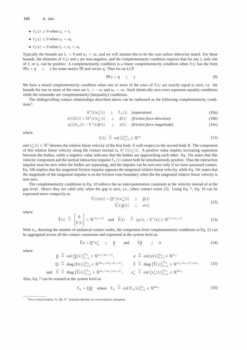
Figure 3. Fully augmentedmodel with hinges modeled asconstraints.

In this section we derive the commonly used non-minimal coordinate LCP formulation forcontact dynamics based on the approach in [3]. We refer to this formulation as thenon-minimal coordinates (NMC)formulation.

Contact and collision dynamics models build upon smooth dynamics models. Thesmooth dynamics model used by the NMC method treats all the links in the system asindependent bodies, and all coupling hinges as explicit bilateral constraints as illustratedin Figure 3. Such a smooth dynamics model utilizes non-minimal coordinates and is alsoreferred to as afully augmented (FA)model [11].

Letn denote the number of links in the system, andN the number of system degrees offreedom in the absence of bilateral constraints. For the FA modelN = 6n. Letnb denotethe dimension of the bilateral constraints arising from inter-link hinges and loop closureconstraints on the system. Withx denoting the vector of positional and attitude coordinatesfor the links, letV ∈ R6n denote the stacked vector of spatial velocities of all the links.Then there exists aGb(x, t) ∈ Rnb×6n matrix and aU(t) ∈ Rnb vector that define thefollowing velocity domain constraint equation for the bilateral constraints on the system:

Gb(x, t)V = U(t) (17)

We assume thatGb(x, t) is a full-rank matrix. Observe that Eq. 17 is linear inV. The bilateral constraints effectivelyreduce the independent degrees of freedom for the system from N to (N − nb). The bilateral constraints are accountedfor via Lagrange multipliers, λ ∈ Rnb to yield the following smooth equations of motion for the system

Mα−G∗b(x, t)λ = C(x,V)

Gb(x, t)V = U(t)(18)

whereα ∈ R6n denotes the spatial acceleration of the bodies.M ∈ R6n×6n is a block diagonal matrix with the 6× 6spatial inertias of each of the links along the diagonal.C ∈ R6n is a vector of the velocity dependent Coriolis andexternal forces on the system. The−G∗

b(x, t)λ term in the first equation represents the constraint forces from the bilateralconstraints. Differentiating the Eq. 17 constraint equation, Eq. 18 can be rearranged into the following descriptor form:

(M −G∗

b

Gb 0

)[α

λ

]=

[C

U

]where U

= U − GbV ∈ Rnb (19)

An attractive feature of these smooth equations of motion isthat theM matrix is block diagonal and constant. Using thefollowing discrete time Euler step approximation over a∆t time interval,2

V+ − V− = α∆t and pb= λ∆t ∈ Rnb (20)

the differential form of the equations of motion in Eq. 19 canbe transformed into the following discretized version thatmaps thepb impulse stacked vector at the bilateral constraint nodes into the resulting change in body spatial velocities.

(M −G∗

b

Gb 0

)[V+ − V−

pb

]=

[C∆t

U∆t

](21)

3.1 Including contact impulses

The stacked vector of relative linear velocities across thecontact nodes is denotedvu ∈ R3nu . It is related to the stackedvector of body spatial velocitiesV via the following relationship

vu = GuV (22)

where theGu ∈ R3nu×6n matrix contains one block-row per contact node-pair, with each row mapping the spatialvelocities for a node pair into the relative linear velocityacross the contact. TheGu matrix also relates theFu equal

2The− and+ superscripts denote the respective value of a quantity justbefore and after the application of an impulse.

A. Jain 167

and opposite impulses at the contact node-pairs to the corresponding spatial impulses on the bodies,pu ∈ R6n via thefollowing dual mapping

pu = G∗uFu (23)

Thepu contact impulses can be included in the Eq. 21 smooth equations of motion by addingpu to theC∆t term toobtain (

M −G∗b

Gb 0

)[V+ − V−

pb

]=

[C∆t + pu

U∆t

](24)

3.2 Assembling the system LCP

We now set up an LCP to help solve the equations of motion and the the unknown constraint forces. From Eq. 16 andEq. 23 we have

Fu = Dβ ⇒ pu = G∗uDβ (25)

Thus Eq. 24 can be recast as(M −G∗

b −G∗uD

Gb 0 0

)V+ − V−

pb

β

=

[C∆t

U∆t

](26)

Combining this with the complementarity conditions in Eq. 14 leads to the following NMC formulation of the LCP inEq. 9:

M=

M −G∗b −G∗

uD 0

Gb 0 0 0

D∗Gu 0 0 E

0 0 E 0

, z

=

V+

pb

β

σ

, q

=

−MV− − C∆t

−GbV− − U∆t

0

0

(27)

This is a mixed LCP problem, where the first two rows are equality conditions, while the lower two rows are comple-mentarity conditions. This NMC LCP formulation is essentially the one described in [3]. It makes use of non-minimalcoordinates for the articulated system and is of size(6n+ nb + nu(nf + 2)). The constant and block-diagonal structureof M results inM having a simple and highly sparse structure. The complexityof assemblingM andq for the LCP isjustO(n). Reference [3] derives sufficient conditions for the existence of a solution for the LCP problem.

The solution of the Eq. 27 LCP provides newV+ velocity coordinates which can be numerically integrated to prop-agate thex configuration coordinates. The solution values ofβ indicate which contacts are active or inactive, while thevalues ofσ define the rolling or sliding state of each of the active contacts. Thus an LCP solution withFu(i) positiveindicates that theith contact isactive. Furthermore,σ(i) = 0 implies that theith contact is arolling contactwhile apositive value implies that it is aslidingcontact.

In the NMC formulation, the LCP does virtually all the work, and the complexity of setting up the LCP is relative low.The main disadvantage of this formulation is the large size of the LCP and the consequent large complexity of solving it.Moreover, the use of non-minimal coordinates requires the additional use of constraint

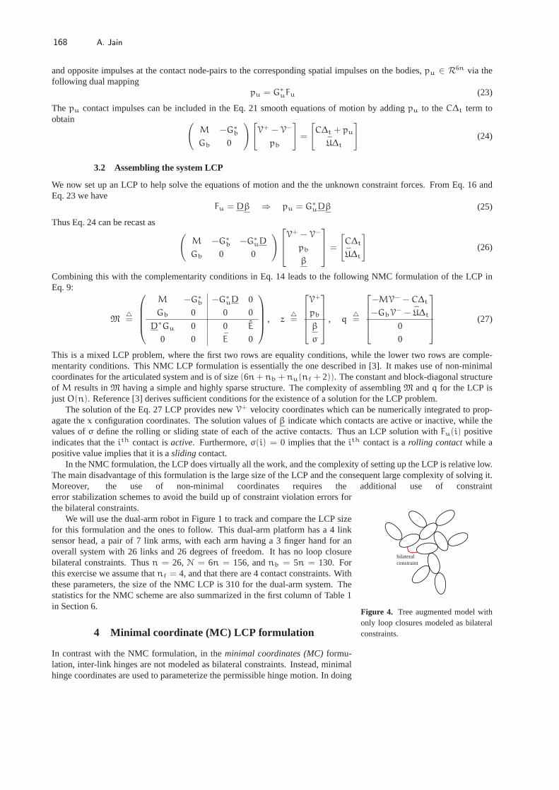
bilateralconstraint

Figure 4. Tree augmented model withonly loop closures modeled as bilateralconstraints.

error stabilization schemes to avoid the build up of constraint violation errors forthe bilateral constraints.

We will use the dual-arm robot in Figure 1 to track and comparethe LCP sizefor this formulation and the ones to follow. This dual-arm platform has a 4 linksensor head, a pair of 7 link arms, with each arm having a 3 finger hand for anoverall system with 26 links and 26 degrees of freedom. It hasno loop closurebilateral constraints. Thusn = 26, N = 6n = 156, andnb = 5n = 130. Forthis exercise we assume thatnf = 4, and that there are 4 contact constraints. Withthese parameters, the size of the NMC LCP is 310 for the dual-arm system. Thestatistics for the NMC scheme are also summarized in the firstcolumn of Table 1in Section 6.

4 Minimal coordinate (MC) LCP formulation

In contrast with the NMC formulation, in theminimal coordinates (MC)formu-lation, inter-link hinges are not modeled as bilateral constraints. Instead, minimalhinge coordinates are used to parameterize the permissiblehinge motion. In doing

168 A. Jain

so, the number of coordinates associated with the hinge match the number of degrees of freedom for the hinge. Thisapproach is used for all the hinges in a spanning tree for the system graph, and bilateral constraints are used only foradditional loop closures that may be present in the system topology as illustrated in Figure 4.

Except for the switch from non-minimal to minimal coordinates, the development of the MC formulation largelyparallels that for the NMC formulation. Hence wherever possible, we reuse the earlier notation, with the understandingthat the meaning of the symbols depends on the formulation context. Thus once again, we useN to denote the numberof degrees of freedom for the tree sub-system. Withθ ∈ RN denoting the vector of hinge coordinates, the minimalcoordinates equations of motion for the smooth dynamics of just the tree-topology sub-system can be expressed as

M(θ)θ+ C(θ, θ) = T (28)

where the configuration dependent matrixM(θ) ∈ RN×N is themass matrixof the system,C(θ, θ) ∈ RN denotes thevelocity dependent Coriolis and gyroscopic forces vector,andT ∈ RN denotes the applied generalized forces. The massmatrix is symmetric and positive-definite for tree-topology systems. The configuration dependency and dense structureof M makes it clearly more complex than the sparse structure and constant value of theM mass matrix in the NMCformulation. On the other hand, for the dual-arm robot system in Figure 1,M is a compact 26-dimensional square matrixcompared with the 156-dimensional square matrixM.

Let nb denote the dimension of the bilateral constraints on the system arising from the loop closures in the system.Sincenb applies only to loop bilateral constraints, it is much smaller thannb in the MC formulation. There exists aGb(θ, t) ∈ Rnb×N matrix and aU(t) ∈ Rnb vector that defines the velocity domain constraint equationas follows:

Gb(θ, t)θ = U(t) (29)

Once again we assume thatGb(θ, t) is afull-rank matrix.The smooth dynamics of closed-chain systems can be obtainedby modifying the tree system dynamics in Eq. 28 to

include the effect of the bilateral constraints viaLagrange multipliers, λ ∈ Rnb , as follows

M(θ)θ+ C(θ, θ) −G∗b(θ, t)λ = T

Gb(θ, t)θ = U(t)(30)

By differentiating the bilateral constraint equation Eq. 29, and including in the average force from thepu ∈ RN contactimpulse, Eq. 30 can be rearranged into the following descriptor form:

(M −G∗

b

Gb 0

)[θ

λ

]=

[T − C+ pu/∆t

U

]where U

= U(t) − Gbθ ∈ Rnc (31)

Using the discrete Euler step approximationθ+ − θ− = θ∆t (32)

the discretized version of Eq. 31 takes the form(

M −G∗b

Gb 0

)[θ+ − θ−

pb

]=

[(T − C)∆t + pu

U∆t

]with pb

= λ∆t (33)

With Gu ∈ R3nu×N such thatvu = Guθ (34)

the dual expression for the contact spatial impulses is given by

pu = G∗uFu

16= G∗

uDβ (35)

Combining the complementarity conditions in Eq. 14 with Eq.33 leads to the MC formulation version of the Eq. 9 LCPwith

M=

M −G∗b −G∗

uD 0

Gb 0 0 0

D∗Gu 0 0 E

0 0 E 0

, z

=

θ+

pb

β

σ

, q

=

−Mθ− − (T − C)∆t

−Gbθ− − U∆t

0

0

(36)

A. Jain 169

This is a mixed LCP with the top two rows correspond to equality conditions while the lower two are complementarityconditions. Its structure is very similar to the NMC formulation LCP in Eq. 27 and differs primarily in the use of minimalcoordinates. The size of the MC LCP is(N + nb + nu(nf + 2)). Unlike the NMC formulation, this dimension does notdepend on the number of linksn. SinceN is much smaller when using minimal coordinates, the MC LCP size is muchsmaller than the NMC LCP size. For the dual arm robot in Figure1, the dimension of the MC LCP is just 50 comparedwith 310 for the NCP formulation.

On the other hand, evaluatingM for the MC LCP requires the configuration dependent and denseM matrix. Whilethe composite rigid body inertia algorithm provides an efficient way to computeM [8], the computational complexityscales asO(N2). Thus the decrease in the LCP size and solution complexity for the MC formulation are accompanied byan increase in the complexity of setting up the LCP. The cost complexity for the MC formulation is also summarized inTable 1. The solution of the MC LCP yields the newθ+ generalized velocity value which can be integrated to propagatetheθ configuration coordinates. As in the case of the NMC formulation, the bulk of the computational effort in the MCformulation is in setting up and solving the LCP problem.

5 Reduced minimal coordinate (RMC) LCP formulation

Continuing with the minimal coordinate approach, we now take further steps to reduce the size of the LCP problem. Thematrix on the left of Eq. 31 can be inverted to yield the following solution forθ:

θf= M−1 [T − C+ pu/∆t] (37a)

λ =[GbM

−1G∗b

]−1(−Gbθf + U) (37b)

θ = θf +M−1G∗b λ

37b=

[I−M−1G∗

b

[GbM

−1G∗b

]−1Gb

]θf +M−1G∗

b

[GbM

−1G∗b

]−1U (37c)

Using Eq. 32, we obtain

θ+32= θ− + θ∆t37c= θ− +

[I−M−1G∗

b

[GbM

−1G∗b

]−1Gb

]∆tθf +M−1G∗

b

[GbM

−1G∗b

]−1∆tU

37a= Ypu + X

(38)

whereY

= M−1 −M−1G∗

b(GbM−1G∗

b)−1GbM

−1 ∈ RN×N

and X= θ− + Y(T − C)∆t +M−1G∗

b

[GbM

−1G∗b

]−1U∆t ∈ RN

(39)

ThusD∗v+u

34= D∗Guθ

+ 35,38= D∗GuY G

∗uDβ+D∗GuX (40)

Using this allows us to eliminateθ+ andpb from the MC LCP formulation in Eq. 36 to obtain the followingReducedMinimal Coordinate (RMC)formulation LCP:

M=

(D∗GuY G∗

uD E

E 0

), z

=

[β

σ

], q

=

[D∗GuX

0

](41)

Since there are no equality conditions, this is a standard rather than a mixed LCP. The size of this RMC LCP isnu(nf+2).It is notable that the size of the LCP does not depend on the number of linksn, the number of degrees of freedomN, nor thenb dimension of the bilateral constraints. It only depends on the number of contact constraint nodes. Thus the dimensionof this LCP is even smaller than that for the MC formulation. For the dual arm robot system, the dimension of the LCP is24. On the other hand, computingM for the RMC LCP requires theY matrix in Eq. 39, which requires the configurationdependentM−1 matrix and several expensive matrix/matrix products. These computations are ofO(N3) computationalcomplexity. Once again, while the RMC formulation has successfully reduced the LCP size and consequently its solutioncomplexity, this reduction has been accompanied by a significant increase in the complexity of setting up the LCP problem.The cost complexity for the RMC formulation is summarized inTable 1.

In contrast with the NMC and MC formulations, the solution ofthe RMC LCP does not by itself yield the new systemvelocity or state. Instead the following sequence of steps is needed to obtain the new state values:

170 A. Jain

1. Assemble and solve the RMC LCP in Eq. 41 to obtainβ andσ. Useβ in Eq. 35 to obtain thepu contact impulsevector.

2. Usepu in Eq. 38 to compute the newθ+ system velocity. This can be integrated to obtain the new system configu-ration coordinatesθ.

Thus, the RMC LCP by itself does not do all the work, and the additional step (2) is needed to complete the computationof the newθ+ system velocity coordinates.

The formulation developed by Trinkle [2] is a hybrid combination of the NMC and RMC formulations. Trinkle’s setupallows the use of general coordinates for describing the smooth equations of motion. However, instead of eliminating thehinge bilateral constraints by using minimal hinge coordinates a pair of symmetric (positive and negative) complemen-tarity conditions are added to enforce the equality condition for each hinge constraint. This inflates the size of the LCPmuch like the NMC approach. However, Trinkle;s approach is similar to the RMC in eliminating the velocity coordinatesand the loop closure bilateral constraint Lagrange multipliers from the LCP problem to obtain an LCP similar in form toEq. 41.

6 Operational space (OS) LCP formulation

So far we have found that the reductions in LCP size have had the side-effect of increasing the LCP setup complexity. Inthis section we look into reducing such setup complexity using low-order articulated system dynamics algorithms. FromEq. 31 we have

029= Gbθ− U

31= GbM

−1 [T − C+G∗bλ+ pu/∆t] − U

= GbM−1G∗

bλ+GbM−1pu/∆t + α

fb where αfb

= GbM

−1(T − C) − U

35= GbM

−1G∗bλ+GbM

−1G∗uDβ/∆t + α

fb

(42)

The above expression characterizes the equality conditionon the dynamics from the bilateral constraints. The relativelinear acceleration of the contact nodes is obtained by differentiating Eq. 34 to obtain

vu = Guθ+ Guθ31= GuM

−1 [T − C+G∗bλ+ pu/∆t] + Guθ (43)

The discretized approximation(v+u − v−u) = vu∆t of this equation leads to

v+u35, 43= GuM

−1G∗bλ∆t +GuM

−1G∗uDβ+ v−u + αfu∆t where αfu

= GuM

−1(T − C) + Guθ (44)

Combining the complementarity conditions in Eq. 14 with Eq.42 and Eq. 44 yields the following mixed LCP for thesystem:

M=

GbM−1G∗

b GbM−1G∗

uD 0

D∗GuM−1G∗b D∗GuM−1G∗

uD E

0 E 0

, z

=

pb

β

σ

, q

=

αfb∆t

D∗(v−u + αfu∆t)

0

(45)

ThisM matrix still requires the configuration dependentM−1 matrix whose evaluation if ofO(N3) computational com-plexity. We next look more closely at the structure of theGu andGb matrices.

The unilateral and bilateral constraints are associated with nodes on the bodies. Let us denote the number of thisoverall set of nodes involved in the unilateral and bilateral constraints asnc. Denoting the spatial velocities of these nodesby the stacked vectorVc ∈ R6nc , there exist matricesQu ∈ R3nu×6nc andQb ∈ Rnb×6nc such that the unilateral andbilateral velocity constraint equations can be expressed as3

vu = QuVc and QbVc = U (46)

Let J ∈ R6nc×N denote the Jacobian for the constraint nodes, so that

Vc = Jθ (47)

3Qu has the same structure as theQb constraint mapping matrix for bilateral constraints for three degree of freedom spherical hinges.

A. Jain 171

It follows from Eq. 29, Eq. 34, Eq. 46 and Eq. 47 thatGu andGb have the following form:

Gu = QuJ and Gb = QbJ (48)

WithΛ

= JM−1J∗ ∈ R6nc×6nc (49)

we can use Eq. 48 to re-expressM in Eq. 45 as

M =

QbΛQ∗b QbΛQ

∗uD 0

D∗QuΛQ∗b D∗QuΛQ∗

uD E

0 E 0

=

[Qb

D∗Qu

]Λ [Q∗

b, Q∗uD]

0

E

0 E 0

(50)

TheΛ = JM−1J∗ matrix definition in Eq. 49 is precisely the mathematical expression for the inverse of theoperationalspace inertiamatrix that is used in the operational space approach for robot manipulation and control [12, 13]. Basedon this structural similarity, we borrow and extend the operational space terminology to our current context with theconstraint nodes forming the operational space nodes. Also, borrowing terminology, we refer toΛ as theoperationalspace compliance matrix (OSCM)matrix. The invertibility ofΛ does not depend onJ being invertible – only thatJ havefull row-rank. When it exists, the inverse ofΛ is referred to as theoperational space inertia. The properties of the OSCMare discussed in detail in [10].

The property of theΛmatrix that is of importance for us is the availability of algorithms ofO(N) +O(n2c) computa-

tional complexity for evaluatingΛ [10, 14]. The low-order of these algorithms is remarkable given the presence ofM−1

in the expression forΛ, since evaluatingM andM−1 individually requireO(N2) andO(N3) computations respectively.This algorithm reduces the complexity of evaluatingM in Eq. 50 fromO(N3) to the much smallerO(N) +O(n2

c) com-putational complexity. The low complexity algorithm for evaluatingΛ is based on an analytical transformation of Eq. 49,followed by a disjoint decomposition of the matrix into block diagonal, and upper and lower triangular components thatcan be computed recursively. A summary of this structure-based analysis and accompanying algorithms using spatialoperator techniques is described in the appendix. An alternative sparsity based technique for evaluatingΛ is described inreference [15].

With θf= M−1(T − C),

αfb42,48= QbJθf − U

31,47= Qb(Jθf + Jθ) + QbVc − U = Qbα

f + QbVc − U

αfu44,48= QuJθf + Gu

47= Qu(Jθf + Jθ) + QuVc = Quα

f + QuVc

(51)

whereαf = Jθf + Jθ (52)

Physically,αf is the stacked vector of spatial accelerations of the constraint nodes in the absence of the bilateral andcontact constraints.

Using Eq. 50 and Eq. 51, the Eq. 45 LCP can be re-expressed as the following Operational Space (OS)formulationLCP:

M=

[Qb

D∗Qu

]Λ [Q∗

b, Q∗uD]

0

E

0 E 0

, z

=

pb

β

σ

, q

=

[Qb

D∗Qu

]∆tα

f +

[Qb

D∗Qu

]∆tVc +

[−U

D∗v−u

]

0

(53)This is a mixed LCP, with the first row corresponding to an equality condition while the bottom two rows correspond tocomplementarity conditions. The size of this LCP is(nb + nu(nf + 2)). Like the RMC formulation, the size of thisLCP does not depend on the number of linksn or the number of degrees of freedomN, but it does depend on thenbdimension of the loop closure bilateral constraints. The dimension of the OS LCP is moderately larger than the RMCLCP but smaller than the MC LCP. Typically,Qu, Qb andU are all zero leading to a simplerq in Eq. 53. For the dual armrobot system, the dimension of the OS LCP is 24.

ComputingM for the OS LCP requires the configuration dependentΛ matrix Eq. 53 whose evaluation is ofO(N) +O(n2

c) computational complexity which is much smaller than theO(N3) complexity for evaluatingM for the RMCmethod. Thus in comparison with the RMC formulation, while the OS formulation increases the size of the LCP by amodestnb, it drastically reduces the LCP setup complexity. The result is a significant reduction in the overall complexityof the contact dynamics computations for the OS formulation.

172 A. Jain

Like the RMC formulations, the solution of the LCP does not byitself yield the new system velocity or state. Insteadthe following sequence of steps is needed to obtain the new state values:

1. Assemble and solve the OS LCP in Eq. 53 to obtainpb, β andσ. Useβ in Eq. 35 to obtain thepu contact impulsevector.

2. Usepb andpu in Eq. 33 to obtain the newθ+ system velocity using theO(N) articulated body forward dynamicsalgorithm. This can be integrated to obtain the new system configuration coordinatesθ.

Like the RMC formulation, the LCP by itself does not do all thework in the OS formulation, but instead the additionalstep (2) is needed to complete the computation of the newθ+ system velocity coordinates.

LCP FormulationProperty NMC MC RMC OS

Coordinates type Non-minimal Minimal Minimal Minimal

LCP assembly complexity O(n) O(N2) O(N3) O(N) +O(n2c)

LCP dimension 6n+ nb + nu(nf + 2) N + nb + nu(nf + 2) nu(nf + 2) nb + nu(nf + 2)

Dual-arm LCP dimension 310 50 24 24

Ancillary dynamics steps None None Evaluatepu andθ+ Evaluatepu andθ+

Table 1. A comparison of the features of the different NMC, MC, RMC and OS formulations for contact and collision dynamics.The LCP dimension size is for the reference dual-arm robot problem, whilethe LCP assembly complexity highlights just the majorcontributors.

The LCP formulation developed by Yamane and Nakamura [7] makes use of thedivide and conquer algorithm (DCA)[16] techniques and is a special case of the OS formulation. The OS formulation here is however more general since ithandles loop closure bilateral constraints, exploits operational space techniques to reduce computational complixity, andas described later, handles collision dynamics.

Table 1 summarizes the dimensions and computational compleixty for all the formulations discussed so far. The trendacross the NMC, MC and RMC formulations is that the reductionin the size of the LCP shifts costs to the LCP setupprocess. While the initial form of the OS formulation LCP in Eq. 45 also follows this trend, the restructured Eq. 53 LCPbreaks the pattern by restructuring the LCP to take advantage of low-order, structure-based algorithms for articulatedsystem dynamics.

7 Collision dynamics

In this section we develop extensions to the OS LCP formulation for handling the dynamics of collision events. Duringinelastic collisions some of the impact energy is lost. Thecoefficient of restitution, ǫ(i) defines the fraction that remainsafter a collision. The complementarity approach to modeling collisions breaks up the collision event into a pair of instan-taneouscompressionanddecompressionphases [3]. During the compression phase, the collision impulse is stored, andduring decompression, a fraction of the collision impulse is recovered. We will make use of time discretized equationswith impulses developed for contact dynamics, but with∆t = 0 since collision events are instantaneous.

7.1 Compression

At theith contact undergoing collision, the compression phase is instantaneous and impulsively changes the relative linearcontact velocity fromv−u(i) to a newv+c (i) value with a non-negative normal component. The compression impulse isdenotedpc(i). The mixed LCP problem for the compression phase is obtainedby setting∆t = 0 in Eq. 53 to obtain

w = Mz+ q ⊥ z with q=

[−U

D∗v−u

]

0

(54)

A. Jain 173

The LCP solution is used to instantaneously (i.e. impulsively) propagate the state for the compression phase as follows:

pc = Q∗uD β+ Q∗

bpb

θc = θ− +M−1J∗pc

v+c = Jθc

(55)

7.2 Decompression

The decompression phase applies an additional impulse of magnitudeǫ(i)[0, n∗(i)pc(i)] for the ith contact along thenormal from the impulse stored during the compression phase. The recoveredϑ decompression impulse is

ϑ= col (ǫ(i)[0, n∗(i)]pc(i)) n(i)

nu

i=1 ∈ R3nu (56)

The decompression LCP is obtained by updating Eq. 42 and Eq. 43 to include the additionalϑ impulse. This leads to adecompression LCP problem that is the mixed LCP in Eq. 53 with∆t = 0, the contact linear velocityv−u replaced with

v+c , and an additional

[Qb

D∗Qu

]ΛQ∗

uϑ term for the recovered impulse included in theq LCP vector term. The resulting

decompression phase LCP is

w = Mz+ q ⊥ z with q=

[−U

D∗v+c

]+

[Qb

D∗Qu

]ΛQ∗

uϑ

0

(57)

The LCP solution for the decompression impulse can include additional contact impulse terms that ensure that the normalcomponent of the relative linear velocity at the end of the decompression step remains non-negative. The LCP solution isused to instantaneously propagate the state for the decompression phase as follows:

p = Q∗uD β+ Q∗

bλ+ Q∗uϑ

θ+ = θc +M−1J∗p(58)

Whenǫ(i) = 0, the collision is completely inelastic, and there is no decompression phase. However, in general, eachcollision event requires the solution of two LCP’s in this approach.

8 Simulation results

We use a simulation of a multi-link pendulum colliding with itself and the environment to quantitatively evaluate the per-formance of the OS formulation. This example also allows us to parameterically measure the performance improvementas a function of the problem dimension by varying the number of links in the pendulum. The environment consists of afloor and a wall located 4m away. The multi-link pendulum consists ofn identical 1kg mass spherical bodies connectedwith pin hinges. The radius of the sphere is scaled based on the number of links to maintain a 12m overall length of thependulum. The pendulum base is located at a height of 10m. Theopen source Bullet software [17] is used for collisiondetection, and the PATH software [18] for solving mixed complementarity problems. The simulation uses a time step of0.1ms, with a 0.5 coefficient of friction and a 0.7 coefficientof restitution to simulate inelastic collisions. The pendulumstarts at an angle ofπ/4 radians with an initial angular velocity of 1 radian/s and agravitational acceleration of 9.8m/s2.

As the pendulum swings from left to right, it collides with the ground, bounces off of the ground, and eventuallycollides with the wall on the right. In the course of the sequence, multiple links are at times in collision with the ground,the wall and with each other. Figure 5 contains a sequence of screen shots from such a simulation for a 12-link pendulum.A video of the simulation is included in the media clips accompanying this article. We have simulated this contact andcollision dynamics scenario using two different techniques. The first technique is the minimal coordinate OS formulationdescribed in Section 6.

The second technique, that we refer to as theNMC/OS formulation, is a non-minimal coordinate variant of the OSformulation. Similar to the NMC method, each link is treatedas an independent body, and the hinges are handled asbilateral constraints between the neighboring links withnb = 6n −N. The NMC/OS LCP has the same form as the OSLCP in Eq. 53, except that the OSCM is the non-minimal coordinateΛ = JM−1J∗, instead of Eq. 49. The NMC/OSΛis a much larger matrix but with a simple block diagonal structure. This NMC/OS LCP does not include system velocitycoordinatesV in z and thus is smaller than the NMC LCP.

174 A. Jain

Figure 5. Time series capture of swinging pendulum simulation with 12 links

The simulation results from the two methods show good agreement. Figure 6 shows example plots of the height andnormal velocity of the last link of the 12-body pendulum fromthe two simulation methods. The vertical spikes in thevelocity plot are discontinuous jumps from collisions involving the pendulum bodies. The small trajectory differences inthe plots decrease further when the time step size is reduced.

Table 2 compares the computational complexity of the OS and the NMC/OS formulations for pendulums with thenumber of links varying between 3 and 30 links. The table alsolists the LCP size for the OS, NMC/OS and the NMCformulations. The size of the LCP remains a constant value of24 for the standard OS formulation even when the number

LCP size Computation Time (s)

Number of links OS NMC/OS NMC OS NMC/OS Speed up

3 24 39 57 13.33 47.79 3.6

6 24 54 90 10.50 68.71 6.5

12 24 84 156 19.06 305.28 16.1

15 24 99 189 21.76 558.10 25.6

24 24 144 288 38.20 1899.86 49.7

30 24 174 354 73.74 4100.51 55.6

Table 2. A comparison of the LCP size and computational time for the OS and NMC/OS formulations for the multi-link pendulumexample with different number of links. The LCP size assumes 4 contacts andnf = 4. The three LCP size columns are for the OS, theNMC/OS and the NMC formulations. The speed up value is the ratio of the NMC/OSto the OS formulation simulation times.

A. Jain 175

Figure 6. Comparisons of the height and normal velocity of the last link using the OS (red) and NMC/OS (blue) formulation basedsimulations for a 12-body pendulum.

of links and degrees of freedom in the system is increased. Incontrast, the LCP size increases with the increase in thenumber of links and degrees of freedom for the NMC/OS and the NMC formulations. We also observe that the OSmethod is about 3.6 times faster for the 3 link pendulum case,and over 55 times faster for the 30 link pendulum whencompared with the the NMC/OS method. The performance gap widens substantially as the number of links in the systemis increased. The performance gap between the OS and NMC formulations will be even greater due to the even larger sizeof the NMC LCP.

We have also applied the OS formulation to simulate manipulation tasks for the dual arm system in Figure 1. Videoclips showing the dual arm removal of a wheel from its hub, andthe grasping and hand off of an impact driver fromone hand to the other in simulation are included in the accompanying media clips. In each of these cases, the contactand collision dynamics events during grasping and other interactions are simulated using the OS formulation. Unlike theserial-chain structure of the pendulum system, the dual-arm system has a more general tree-topology.

9 Conclusions

In this article we have described a progression of formulations for the contact and collision dynamics of multi-link artic-ulated systems with the goal of reducing computational complexity. Along the way, we have clarified the relationshipsamong the different approaches and those in the literature.Our strategy has been to find a formulation that best exploitsthe available low-order articulated body dynamics algorithms to reduce the overall computational complexity.

The formulations studied here vary in the size of the LCP, thecomplexity of setting up the LCP, and the ancillarydynamics steps needed to complete the dynamics solution. The generally observed trend is that the reduction in the LCPsize shifts the computational burden from solving the LCP problem, to the setting up of the LCP problem. The widely usedNMC non-minimal coordinate formulation is the simplest andcheapest to set up, but also the most expensive to solve dueto its large dimension. The RMC minimal coordinate approachon the other hand has the smallest LCP dimension, but onethat is the most expensive to set up. In the RMC approach, the size of the LCP problem in is just(nu(nf+2)+nb), whichis independent of the number of links, the number of degrees of freedom and the dimension of the bilateral constraints onthe system. In contrast, the size of the corresponding NMC LCP is larger by 6n − N. For a 6-link manipulator with 6degrees of freedom, this amounts to difference in dimensionof 30.

The OS formulation shares the small LCP dimension property of the RMC approach, with an LCP that is larger by onlythe modest dimension of the loop closure bilateral constraints,nb. We show that the OS formulation can be restructured ina form that expresses its LCP matrix in terms of the operational space OSCM matrix for the constraint nodes. This insightallows us to apply low-order, structure-based computational algorithms available for the OSCM to significantly reducethe complexity of setting up the OS LCP. Consequently the OS formulation is the lowest overall complexity formulationwith a small LCP along with low complexity algorithms for setting up the LCP. Focusing on this option, we describeextensions of the contact dynamics formulation to handle elastic and inelastic collision dynamics. The OS formulation’suse of minimal coordinates also results in the automatic enforcement of the inter-link hinge bilateral constraints andavoidsthe need for additional bilateral constraint error controlschemes. The benchmark simulations using a pendulum system

176 A. Jain

show a widening performance improvement using the OS formulation as the number of bodies is increased. For the 30 linkpendulum system, the OS formulation is over 55 times faster than the NMC/OS approach. An area of future work is theintegration of the OS formulation with the large variety of time stepping schemes that are in development for increasingthe robustness and accuracy of contact and collision non-smooth dynamics [19].

Acknowledgments

The research described in this paper was performed at the JetPropulsion Laboratory (JPL), California Institute of Technol-ogy, under a contract with the National Aeronautics and Space Administration and funded through the internal Researchand Technology Development program.4

References

[1] D. Stewart and Jeffrey C Trinkle. An implicit time-stepping scheme for rigid body dynamics with Coulomb friction.In Proceedings2000ICRA. Millennium Conference.IEEE InternationalConferenceon RoboticsandAutomation.SymposiaProceedings(Cat.No.00CH37065), pages 162–169. Ieee, 2000.

[2] Jeffrey C Trinkle. Formulation of Multibody Dynamics asComplementarity Problems. InASME InternationalDesignEngineeringTechnicalConference, Chicago, IL, September 2003.

[3] Mihai Anitescu and F A Potra. Formulating dynamic multi-rigid-body contact problems with friction as solvablelinear complementarity problems.NonlinearDynamics, 14(3):231–247, 1997.

[4] F Pfeiffer. Mechanical System Dynamics. Springer, 2005.

[5] Abhinandan Jain, Cory Crean, Calvin Kuo, Hubertus von Bremen, and Steven Myint. Minimal Coordinate Formu-lation of Contact Dynamics in Operational Space. InRoboticsScienceandSystems, Sydney, Australia, 2012.

[6] Alessandro Tasora and Mihai Anitescu. A matrix-free cone complementarity approach for solving large-scale,nonsmooth, rigid body dynamics.ComputerMethodsin Applied MechanicsandEngineering, 200(5-8):439–453,January 2011.

[7] Katsu Yamane and Yoshihiko Nakamura. A Numerically Robust LCP Solver for Simulating Articulated RigidBodies in Contact. InRobotics:ScienceandSystemsIV, chapter A numerica, pages 89–104. MIT Press, 2009.

[8] M W Walker and David E Orin. Efficient Dynamic Computer Simulation of Robotic Mechanisms.ASME Journalof DynamicSystems,Measurement,andControl, 104(3):205–211, September 1982.

[9] Roy Featherstone.Rigid Body Dynamics Algorithms. Springer Verlag, 2008.

[10] Abhinandan Jain.Robot and Multibody Dynamics: Analysis and Algorithms. Springer, 2011.

[11] Abhinandan Jain, Cory Crean, Calvin Kuo, and Marco B. Quadrelli. Efficient Constraint Modeling for Closed-ChainDynamics. InThe2ndJointInternationalConferenceonMultibody SystemDynamics, Stuttgart, Germany, 2012.

[12] Oussama Khatib. Object Manipulation in a Multi-Effector System. In4th InternationalSymposiumon RoboticsResearch, pages 137–144, Santa Cruz, CA, May 1988.

[13] Oussama Khatib. A Unified Approach for Motion and Force Control of Robot Manipulators: The Operational SpaceFormulation.IEEEJournalof RoboticsandAutomation, RA-3(1):43–53, February 1987.

[14] K Kreutz-Delgado, Abhinandan Jain, and Guillermo Rodriguez. Recursive formulation of operational space control.Internat.J.RoboticsRes., 11(4):320–328, 1992.

[15] Roy Featherstone. Exploiting Sparsity in Operational-space Dynamics.Internat.J.RoboticsRes., 29(1992):1353–1368, September 2010.

[16] Roy Featherstone. A divide-and-conquer articulated-body algorithm for parallel O(log(n)) calculation of rigid-bodydynamics. Part 2: Basic algorithm.Internat.J.RoboticsRes., 18(9):867˜875, 1999.

4 c©2013 California Institute of Technology. Government sponsorship acknowledged.

A. Jain 177

[17] Bullet Physics Library, 2013.

[18] The PATH Solver, 2012.

[19] Christian Walter Studer.Augmented time-stepping integration of non-smooth dynamical systems. PhD thesis, ETHZurich, 2008.

[20] Abhinandan Jain. Graph Theoretic Foundations of Multibody Dynamics Part II: Analysis and Algorithms.MultibodySystemDynamics, 26(3):335–365, October 2011.

[21] Guillermo Rodriguez, Abhinandan Jain, and K Kreutz-Delgado. A spatial operator algebra for manipulator modelingand control.Internat.J.RoboticsRes., 10(4):371, 1991.

10 Appendix

The operational space for the multi-link system is defined bythe configuration of the set of constraint nodes on the system.The key implementation and computational challenge for setting up the OS formulation LCP in Eq. 53 is the need forevaluating theΛmatrix. As seen in Eq. 49,Λ involves the configuration dependent matrix products of theJacobian matrixand the mass matrix inverse. A direct evaluation of this expression requiresO(N3) computations. However references[10, 14, 20] have used spatial operators to develop simpler and recursive computational algorithms forΛ that are of onlyO(N) complexity. We briefly describe the underlying analysis andstructure of this algorithm, and refer the reader to[10, 14, 20] for notation and derivation details.

10.1 Spatial operator factorization of M−1

We begin with the following key spatial operator based analytical results that provide explicit, closed-form expressionsfor the factorization and inversion of a tree mass matrix [10, 21]:

M = HφMφ∗H∗

M = [I+HφK]D [I+HφK]∗

[I+HφK]−1 = [I−HψK]

M−1 = [I−HψK]∗ D−1 [I−HψK]

(59)

The first expression defines the Newton-Euler operator factorization of the mass matrixM in terms of theH hinge artic-ulation, theφ rigid body propagation and theM link spatial inertia operators. While this factorization has non-squarefactors, the second expression describes an alternative factorization involving only square factors with block diagonalDand block lower-triangular[I+HφK] matrices. This factorization involves new spatial operators that are associated withthearticulated body (AB)forward dynamics algorithm [9, 20] for the system. The next expression describes an analyticalexpression for the inverse of the[I + HφK] operator. Using this leads to the final analytical expression for the inverseof the mass matrix. These operator expressions hold generally for tree-topology systems irrespective of the number ofbodies, the types of hinges, the specific topological structure, and even for non-rigid links [10].

10.2 TheΩ extended operational space compliance matrix

With V ∈ R6n denoting the stacked vector of link spatial velocities, itsspatial operator expression is [10]

V = φ∗H∗θ (60)

Bundling together the rigid body transformations for all nodes we define theB ∈ R6n×6nc pick-offmatrix such that thestacked vector of node spatial velocitiesVc can be expressed as

Vc = B∗V60= B∗φ∗H∗θ ⇒ J

47= B∗φ∗H∗ (61)

This is the spatial operator expression for theJ Jacobian matrix. Using this expression and Eq. 59 for the mass matrixinverse within Eq. 49 leads to the following expression forΛ:

Λ49= JM−1J∗ 59

= B∗φ∗H∗(I−HψK)∗D−1(I−HψK)HφB (62)

178 A. Jain

Using the spatial operator identity [10, 21](I−HψK)Hφ = Hψ (63)

in Eq. 62 leads to the following simpler expression forΛ:

Λ = B∗ΩB withΩ= ψ∗H∗D−1Hψ ∈ R6nc×6nc (64)

We have arrived at an expression forΛ, that unlike Eq. 49, involves neither the mass matrix inverse nor the node’s Jacobianmatrix! We refer toΩ as theextended operational space compliance matrix. This terminology is based on Eq. 64 whichshows that the OSCM,Λ can be obtained by a reducing transformation of the full, allbodyΩ matrix by theB pick-offoperator involving just the matrix sub-blocks associated with the parent links of the nodes. From its definition, it is clearthatΩ is a symmetric and positive semi-definite sinceD−1 is a symmetric positive-definite matrix.

While the explicit computation ofM−1 or J is not needed to obtainΛ, the direct evaluation of Eq. 64 still remains ofO(N3) complexity due to the need for carrying out the multiple matrix/matrix products. The next section shows that thesematrix/matrix products can be avoided by exploiting a decomposition of theΩmatrix.

10.3 Decomposition ofΩ

The following lemma describes a decomposition ofΩ into simpler component terms and an expression for its blockelements. TheE∗

ψ andψ() terms used below are defined in references [10, 20]. Furthermore,℘(k) denotes the parent linkfor thekth link, andi ≺ j notation implies that thejth link is an ancestor of theith link in the tree.

Lemma 1 Decomposition ofΩΩ can be decomposed into the following disjoint sum:

Ω = Υ+ ψ∗Υ+ Υψ+ R where R=

∑

∀i,j: i⊀⊁jk=℘(i,j)

eiψ∗(k, i)Y(k)ψ(k, j)e∗

j(65)

Υ ∈ R6nc×6nc is a block-diagonal operator, referred to as the operational space compliance kernel, satisfying thefollowing backward Lyapunov equation:

H∗D−1H = Υ− diagOfE∗ψΥEψ

(66)

diagOfE∗ψΥEψ

represents just the block-diagonal part of the (generally non block-diagonal)E∗

ψΥEψ matrix. The

6 × 6 dimensional, symmetric, positive semi-definiteΥ(k) diagonal matrices satisfy the following parent/child recursiverelationship:

Υ(k) = ψ∗(℘(k),k)Υ(℘(k))ψ(℘(k),k) +H∗(k)D−1(k)H(k) (67)

This relationship forms the basis for the followingO(N) base-to-tips scatter recursion for computing theΥ(k) diagonalelements:

for all nodesk (base-to-tips scatter)

Υ(k) = ψ∗(℘(k),k)Υ(℘(k))ψ(℘(k),k) +H∗(k)D−1(k)H(k)

end loop

(68)

WhileΥ defines the block-diagonal elements ofΩ, the following recursive expressions describe its off-diagonal terms:

Ω(i, j) =

Υ(i) for i = j

Ω(i,k)ψ(k, j) for i k ≻ j, k = ℘(j)

Ω∗(j, i) for i ≺ j

Ω(i,k)ψ(k, j) for i ⊁ j, j ⊁ i, k = ℘(i, j)

(69)

Proof: See [10, 20].

Eq. 65 shows thatΩ can be decomposed into the sum of simpler terms consisting ofthe block diagonalΥ, the upper-triangularψ∗Υ, the lower triangularΥψ, and the sparseR matrices. Furthermore, Eq. 69 reveals that all of the block-elements ofΩ(i, j) can be obtained from theΥ(i) elements of theΥ block-diagonal operational space compliance kernel.

A. Jain 179

From theΛ = B∗ΩB expression, and the sparse structure ofB, it is clear that only a subset of the elements ofΩare needed to computeΛ. TheB pick-off operator has one column for each of the nodes, with each such column havingonly a single non-zero 6× 6 matrix entry at thekth parent link slot. Only as many elements ofΩ as there are elementsin Λ are needed. Thus, justnc × nc number of 6× 6 sub-block matrices ofΩ are required. In view of the symmetry ofthe matrices, we actually need justnc(nc + 1)/2 such sub-block matrices. The overall complexity of this algorithm islinearly proportional to the number of degrees of freedom, and a quadratic function of the number of nodes. This is muchlower than theO(N3) complexity implied by Eq. 49.

180 A. Jain