mispricing persistence and the effectiveness of arbitrage

* I am indebted to Patrick Hazart and Dominique Martin from NYSE-Euronext for providing the data used in this study. I also thank Bruno Biais, Alain François-Heude, Larry Glosten, Nabil Khoury, Patrice Poncet, Chester Spatt, the editors as well as two anonymous referees for valuable comments and suggestions. The usual disclaimer applies.

(Multinational Finance Journal, 2007, vol. 11, no. 1/2, pp.123–156)© Multinational Finance Society, a nonprofit corporation. All rights reserved. DOI: 10.17578/11-1/2-5

1

Mispricing Persistence and the Effectivenessof Arbitrage Trading

Pascal AlphonseLille School of Management, University of Lille 2, France

This article examines whether mean reversion in stock index basis changes isactually induced by arbitrage trading, using intra-day arbitrage trade data. Theempirical evidence suggests that arbitrage trading alone cannot account for allof the mean reversion in basis changes, even when infrequent trading iscontrolled for. This general mean reversion is consistent with mean reversionin liquidity and partial adjustment in the cash market. The behavior ofarbitrageurs appears highly competitive. We find that on average the netarbitrage profit is at the competitive level of zero. Furthermore, it is suggestedthat some mispricing persistence may be related to time-varying liquidity.Accordingly, the results indicate that arbitrageurs pay attention to the depth ofthe market and value the early unwinding option (JEL: G13, G14).

Keywords: market microstructure, arbitrage trading, liquidity, stock indexfutures, market efficiency.

I. Introduction

The mean reversion in stock index futures basis changes is documentedin a number of studies (see for example MacKinlay and Ramaswamy[1988] for the U.S., Yadav and Pope [1990], Yadav and Pope [1994]and Strickland and Xu [1993] for the U.K. and Lim [1992] for Japan).This mean reversion is traditionally viewed as a consequence of activearbitrage trading and appears as a by-product of efficient futurespricing. Recent papers on this topic make this analysis more precise andprovide new indirect evidence—based on price data—of arbitrage

Multinational Finance Journal124

2. To the best of our knowledge, the reasons explaining why arbitrage models behaveso poorly are not well understood. Perhaps that the level of competition in the arbitragesector, as modeled for example by Holden (1990), Lambrecht (2000) and in a more generalsetting by Spatt & Sterbenz (1985), is underestimated.

effectiveness. For example, Yadav and Pope (1998) suggests that themean-reversion characterizes changes in the basis when the futures pricehit some trigger points only, due to transaction costs. Then, Yadav andPope (1998) describes the behavior of the basis as a thresholdautoregressive process. Following Kawaller (1991), Tse (2001) arguesthat transaction costs differ among arbitrageurs and suggests that thearbitrage sector should not be reduced to a representative arbitrageur.He shows that the observed mean reversion in mispricing changes isinduced by heterogeneous arbitrageurs and shows that a smoothtransition autoregressive process provides a better description of themispricing behavior than the traditional threshold process. The samearguments are presented in Dwyer, Locke and Yu (1996). Likewise,Kempf (1998) examines the impact of short selling restriction and earlyunwinding opportunities on the dynamics of the mispricing.

Miller, Muthuswamy and Whaley (1994), however, challenges thistraditional view of arbitrage trading and argues that infrequent tradingin the stock market is a sufficient condition for the basis to exhibit somemean reversion. More recently, Theobald and Yallup (2001) argues thatpartial adjustment to new information leads to negative autocorrelationsin basis innovation series. Lead-lag relationships between futures andspot prices constitutes a natural support for this partial adjustment.Finally, Neal (1996) shows that the traditional determinants of arbitragetrading (mispricing level and mispricing sign, time to expiration, earlyliquidation option) explain only a very low proportion of actualarbitrage trades. That is, arbitrage trading may not be as predictable assuggested in the works cited above.2 Thus, the prominent role attributedto arbitrage trading may in fact be driven by a misleading proxy foractual arbitrage trading and by indirect inference about arbitrageeffectiveness. One way to cope with this difficulty is to base the resultsconcerning the relationship between arbitrage trading and meanreversion in basis changes on actual arbitrage trades. This directinference is the subject of this paper where the mean reversion inmispricing changes is examined using actual data on arbitrage tradingon Euronext Exchange.

More precisely the paper makes two contributions to the existingliterature on arbitrage trading and mispricing behavior.

125Mispricing Persistence & Arbitrage Trading

3. It does not mean that all of the serial dependance is removed from the index series.It suggest that if the index series still exhibit some serial dependancy, then it must be relatedto information dissimination across the stocks and to price adjustments (e.g., Chan [1993]),not to cross sectional differences in trading frequency across the stocks.

4. See in a related context the analysis in Cheung and Fung (1997).

First, the results indicate that mispricing is not persistent becausearbitrage opportunities are rapidly exploited by stock index arbitrageursbut also because of some general, non-arbitrage mean reversion inmispricing changes. This result is not evidence of some statisticalillusion of the type defined by Miller, Muthuswamy and Whaley (1994)because we use quotes instead of transaction prices to compute theindex. As a result the index value is not biased by some stale priceeffect induced by infrequent trading.3

It is suggested that this non-arbitrage mean reversion may be drivenby (non-informational) liquidity shock, by partial quote adjustment inthe cash market and by the lead-lag relationships between the futuresand the stocks. The liquidity shock explanation is reminiscent to Krausand Stoll (1972) who shows that large trades cause price reversals(reflected here in reversion in the basis) and is also consistent with theoverbidding/undercutting strategies documented in Biais, Hillion andSpatt (1995).

The partial quote adjustment in the cash market may be induced bylimit order traders that do not always respond to changes infundamentals by instantaneously adjusting the quotes. This is consistentwith observed stale quotes in the cash market and with the partialadjustment model of Theobald and Yallup (2001). Finally, according tothe lead-lag explanation, it is possible that new information isimpounded in one market first, say the futures market, causing anincrease in the mispricing, and that stock market traders observing thefutures price adjust their quotes, which decreases the value of themispricing.4 Thus, one would naturally expect some mean reversion totake place without arbitrage trading.

The existence of non-arbitrage mean reversion in the basis changesdeparts from the recent results of Kempf (1998) or Tse (2001). Thisresult may come from the fact that arbitrage trading is actually found tobe far less frequent and predictable that it would be found by applyingsome mechanical trading rules. These data characteristics are notspecific to our sample (see for example the description of the arbitragedata in Harris, Sofianos and Shapiro [1994]) and then must be related


to some determinants of arbitrage trading.Second, the results indicate that the liquidity of the market, and

especially the depth is a key determinant of arbitrage trading. To thebest of our knowledge, this is the first time that the depth (in additionto the spread) is used as a determinant of arbitrage trading. Neal (1996)documents time variation is spread and suggests that it is related toarbitrage trading. Nevertheless, it should be the case that arbitrageursare aware of the quantity of shares they can trade for a given price, thedepth of the market. This is consistent with the arbitrage models ofKumar and Seppi (1994), Holden (1990, 1995) and Fremault (1991). Itis also shown that in establishing an arbitrage position an arbitrageurtakes into account the possibility to reverse rapidly the trade. Weprovide new evidence consistent with the early-liquidation option modelof Brennan and Schwartz (1990). Finally, our results are consistent withwhat one would expect theoretically if arbitrageurs were 100% certainbeing able to unwind their position prior to the maturity date andcompetition among arbitrageurs had eliminated all excess rents. That is,we find that on average, the net arbitrage profit is at the competitivelevel of zero. Liquidity and time-variation in mispricing series mayexplain part of the dispersion observed in arbitrage trigger points.

The present paper is closely related to the papers due to Neal (1996)and Harris, Sofianos and Shapiro (1994) in that the three papersdocument and characterize a set of arbitrage orders. Nevertheless theanalysis presented in this paper differs from these previous studies inseveral ways. First, a new and more recent dataset related to ascreen-based, order-driven market in which the supply of liquidity relieson limit order traders only is used. The comparison with the U.S. caseis interesting and may contribute to the debate on the ability of differenttrading systems to provide some heterogeneous classes of investors withliquidity (e.g., Venkataraman [2001]).

Second, the rules governing short sale constraints are also differentin the U.S. and France. As shown in numerous papers, these rules affectthe opportunity cost of funds (Kawaller [1991], Kempf [1998]), andthen the arbitrage decision. In particular, we discuss the impact of theaccount settlement mechanism.

The size of the index is a third difference between the present studyand the two others that use arbitrage data (Neal [1996] and Harris,Sofianos and Shapiro [1994]). The CAC 40 index is based on 40 stocksversus the 500 stocks of the S&P. This difference may induce lessinfrequent trading, mimicking strategies and tracking errors so arbitrage


5. For an analysis of these features and their impacts on stock index futures valuation,see McDonald (2001) and Theobald and Yallup (1996).

in the French case may be less risky and the data more homogeneousthan in the U.S. With respect to the size of the index, this paper is morerelated to Tse (2001), but using arbitrage data.

Fourth, as in Neal (1996) and Harris, Sofianos and Shapiro (1994),evidence of mean reversion induced by arbitrage trading is presented.However, the hypothesis that mean reversion in stock index basischanges is not induced by arbitrage trading only is also examined. Thisis a particularly important issue of this paper because, to the best of ourknowledge, none of the papers that deals with this latter question(Kempf [1998], Tse [2001]) uses (arbitrage) trade data. As previouslystated, this would be without consequences if arbitrage trading was aperfectly deterministic function of the mispricing, but it is not.

Fifth, the analysis of the determinants of arbitrage tradingemphasizes the role of the liquidity, especially the depth of the market,and computes variables related to the arbitrage order imbalance and tothe (expected) reversion in the basis in order to address the hypothesisof the early liquidation option.

The rest of the paper is organized as follows. The methodology ispresented in section II. The data and the markets are described in sectionIII. Section IV provides an analysis of the arbitrage order flow.Regression results are presented in section V. Section VI concludes.

II. Research Methods

The fair value of the futures is obtained by applying the traditionalcost-of-carry model adapted for the specificities of the French stockmarket, the fixed-date settlement and the dividend tax credit systems.5

Mispricing is defined as in Mackinlay and Ramaswamy (1988) by thedifference between the actual (Ft,T) and theoretical prices (F*

t ,T) of afutures with maturity T priced at time t and divided by the current indexvalue (St):

(1), ,,

t T t Tt T

t

F FMIS

S

∗−=

Mispricing is also defined and measured with respect to deviations from


6. Brennan and Schwartz (1990), page 18.

an arbitrage-free range defined from bid and ask quotes. Let F*Ask,t,T and

F*Bid,t,T be the theoretical prices of a futures contract with maturity T

evaluated at time t with the bid and ask stock quotes. The position of theactual price of a futures with maturity T in this arbitrage-free range ismeasured at time t by the variable θt,T defined as:

(2). , ,,

, , , ,

t T Bid t Tt T

Ask t T Bid t T

F F

F Fθ

∗

∗ ∗

−=

−

If the actual futures price is at time t between the theoretical bid and askvalues of the futures, then 0#θt,T#1, whereas long (cash and carry)arbitrages should be associated with θt,T#1 and short (reverse cash andcarry arbitrages) with θt,T#0.

Nevertheless, we may note that, while the standard arbitragecondition implies that no arbitrage order should be submitted when theprice of the futures stands in this price range, the presence of arbitrageorders within this range is consistent with arbitrageur valuing an optionto unwinding their position before the maturity date. As stated byBrennan and Schwartz (1990), “it may be optimal to open a newarbitrage position even when the simple arbitrage profit is less than thecost of executing the simple arbitrage. The reason for this is that asimple arbitrage position carries with it an option to close out early andthereby make an additional arbitrage profit”.6 The empirical analyses inSofianos (1993) and Neal (1996) support this view for the U.S. markets.

Furthermore, one may expect all the arbitrage positions to happen incluster at some unique trigger point less than θt,T = 1 for cash and carryarbitrage (and at some unique trigger point greater than θt,T = 0 forreverse cash and carry arbitrage) only if all the arbitrageurs value theunwinding option in the same way. On the contrary, difference in thevaluation of the unwinding option should result in some dispersion ofthe arbitrage position inside the traditional “establish and hold tomaturity” arbitrage trigger points (θt,T = 1 and θt,T = 0). Differences inthe valuation of the unwinding option may come from differences inposition limits (Brennan and Schwartz [1990]), differences intransaction costs (Kawaller [1991] and Tse [2001]) or strategic behaviorin an oligopolistic arbitrage sector (Lambrecht [2000]).

In order to assess the effective role of arbitrage trading in the mean


7. See also Kempf (1998) for the use of the ADF type regression in an analysis of themispricing behavior.

reverting process of the basis we have estimated the followingAugmented Dickey-Fuller type regression :7

(3)4

11 1

p

t t i i t i t j ti j

MIS TTM D MIS MISα β γ φ ε− −= =

Δ = + + + Δ +∑ ∑

where TTM denotes the time-to-maturity in days, MIS is the mispricingvalue and ΔMIS is the first difference in MIS. The time-to-maturityvariable is included to account for the possibility of mean reversionaround a time-dependent value.

The effective role of arbitrage trading is tested allowing for dummyvariables Dt in the regression. More specifically, if a long arbitrageposition is established at time t then D1 = 1and if a short arbitrageposition is established then D2 = 1. If there is no arbitrage trading attime t then D3 = 1 for positive mispricing and D4 = 1 for negativemispricing. Hence at each time t there is only one dummy that is equalto one and the other dummies are zero. We have also included p laggedmispricing changes in the regression equation in order to correct forautocorrelation in mispricing changes.

Finally, a logit model is estimated in order to test for the significancevariables that may be related to arbitrage trading models. First of all, theabsolute value of the mispricing at time t is retained as the maintraditional determinant of arbitrage behavior (ABSMIS). As suggestedby numerous papers, it may be the case that the required mispricing inestablishing an arbitrage position is larger in case of reverse cash andcarry than in cash and carry. The rule governing short sale constraintsin France which are presented in the next section suggests that it wouldalso be case in France. To test this hypothesis a dummy for negativemispricing (NEGMIS) is included. A positive relationship betweenarbitrage trading and these two variables is expected.

In order to take into account the influence of the persistence ofmispricing on arbitrage trading, a time-stamped measurement of theduration of the mispricing (DURATION) is included in the model. Theconstruction of this variable is explained below.

Data are sampled and the mispricings are indexed by their ranks insome sequences of successive positive, negative or zero mispricings.


8. There is no guideline for the choice of this duration. We chose seven trading hoursbecause it is the duration of a trading day. Alternatives have been tested and showed that theresults are not dependent on this particular choice.

Thus, each mispricing is the nth mispricing of a typical period of over-,under- or fair valuation of the futures. The duration of a mispricing attime t is then defined as its rank at that time in a given mispricingperiod.

The hypothesis tested is that arbitrage trading is positivelyassociated with this duration. The intuition is that it may take time fora mispricing value to become large enough to induce arbitrage trading.This delay may be caused for example by the conjunction of a fine pricegrid (a small tick size) and a price continuity rule between prices.Arbitrageurs may also look at mispricing persistence in order to gaugethe probability of reversal in the basis (e.g., Chung [1991]) and thus thefeasability of arbitrage.

The opportunity of establishing an arbitrage position may well berelated to the liquidity of the market too. In fact, the amount of moneyearned in arbitrage trading should be related to the number of shares andcontracts that may be traded in establishing the position. Therefore thedepth of the market rather than the spread may be positively associatedwith arbitrage trading. This conjecture is test in consideringsimultaneously the bid-ask spread (SPREAD) and the depth (DEPTH)in the model. It may be noted that we use a directional measure of thedepth in that we consider only the market side associated with the signof the mispricing (depth at the ask for positive mispricing and depth atthe bid for negative mispricing). A positive sign for DEPTH and anegative sign for SPREAD are expected.

Finally, and following Brennan and Schwartz (1990), wehypothesize that in establishing a new position, an arbitrageur isconcerned with the option to liquidate the trade early. Investigations bySofianos (1993) and Neal (1996) indicate that early liquidation is in factthe rule. To test for the presence of such an option value, threeadditional variables are considered: a forward-looking measure ofreversal in the basis (REVERSAL), the time-to-maturity of the futurescontract (TTM) and a measure of arbitrage order imbalance (AOIMB).

The reversal variable is defined as the percentage of reversemispricing over the next seven trading hours.8 For example if the currentmispricing value is positive, then the variable is equal to the percentageof negative mispricing values observed over the next seven trading


9. This situation has changed in September 2001 and all the trades are now settled ona day + 3 basis. Brokers, however, offer investors the possibility to trade on the basis of theSRD (for Système de Règlement Différé) which is a device that mimics the functioning of theold monthly settlement.

hours. This variable may be seen as the arbitrageurs’ expectation abouta future mispricing reversal. This variable is expected to be positivelyassociated with arbitrage trading. The time to maturity of the contractis the number of days before expiration. It should capture at least somepart of the time-varying component of the early liquidation option andis expected to be positively associated with arbitrage trading. Thearbitrage order imbalance is measured by a dummy variable. The lattertakes the value of 1 if the arbitrage that would be associated with thecurrent mispricing value reduces the arbitrage order imbalance resultingfrom previous arbitrage trades, and 0 otherwise. The intuition is thatarbitrageurs may be more favorable in establishing an arbitrage positionif it reduces current arbitrage order imbalance, that is, if they liquidatetheir position early.

III. The Market and the Data

A. The CAC 40 Cash and Futures Markets

The analysis reported in this paper is related to the French stock andstock index futures markets. Until recently, the Paris stock exchangeoperated a system of account settlement, the Réglement Mensuel, or inEnglish, the Monthly Settlement.9 Each year was divided up into twelveaccounts. Accounts were of one-month duration, running from the fifthtrading day preceding the last trading day of the month to the sixthtrading day preceding the last trading day of the following month.Settlement of the trades during an account took place on the account daywhich is the last business day of the month following an account.Hence, normal settlement of trade took place between six days and onemonth and six days after a trade date.

The account settlement system has numerous implications forfutures pricing (for a general treatment see Theobald and Yallup[1996]). One of them concerns short sales. Since all trades during anaccount are settled on the same account day, it gives arbitrageurs anincentive to open and close reverse arbitrage positions in the same


10. This situation changed in spring 1998 and the stock index futures market is now anelectronic market managed by the Liffe.

account. In that case, arbitrageurs sell the stocks short and buy themback later in the same account, with no need to pay a fee for borrowingthe stocks. Nevertheless, when arbitrage positions are closed on thematurity of the futures, arbitrageurs in short position who buy stocks onthat date will not receive the stocks until the relevant account day, thatis about one month later. Thus, they have to borrow the stocks they soldshort for a onemonth period. Therefore, while the account settlementsystem facilitates short sales, it does not eliminate the borrowing costof stocks for most of the reverse arbitrage positions. Furthermore, itintroduces some uncertainty in the return of short arbitrage positionsbecause the borrowing cost is not known at the time the reversearbitrage positions are opened.

The futures market is a traditional open outcry market and the stockmarket is a screen-based, order-driven market.10 This electronic marketoperates without designated market makers so public limit orders are theonly source of market liquidity. The five best bids and offers as well astheir associated depths, except for the hidden limit orders, arecontinuously displayed to traders.

This transparency can affect the strategies of market participants.For example, limit order traders who are the most exposed toasymmetric information may protect themselves by cancelling theirorders and leaving the market, leading to temporary market breakdownsor to high and uncertain transaction costs for arbitrageurs. In thiscontext, the level of available liquidity may affect the timing ofarbitrage trading and the persistence of mispricing. Furthermore, Biais,Hillion and Spatt(1995) indicate that most of the depth is concentratedon the best quotes.

B. The Data

Intra-day arbitrage trading data (which are not publicly available) havebeen obtained from EuroNext for the first quarter of 1995. While wehad expected to access data related to a more recent period, the data setwe obtained and worked on allows us to look at the actual tradingbehavior of arbitrageurs, not their supposed behavior implied by the costof carry model, and then deserves further analysis.

These data indicate the time of the arbitrage order initiation, the side


11. It also appears that the number of active arbitrageurs is limited. Inspection of thearbitrageur data ID shows that about 90% of the orders are submitted by only 15 arbitrageursand the first three of them submit slightly more than one third of the total number of orders.

12. Stale price effects and index autocorrelation should appear as soon as the stocks havedifferent trading frequency.

of the market (cash and carry arbitrage versus reverse cash and carryarbitrage), the number of different stocks in each arbitrage order and themoney value of each arbitrage order.11

A first characterization of these data is provided in section III. Weuse time stamped transaction prices for the CAC 40 futures and intra-day stock quotes for the period from January 3rd, 1995 to March 31st,1995 to compute the theoretical fair value of the futures. The intra-daydata are extracted from the Historical Market Database of EuroNext.The interest rates used to evaluate the cost-of-carry of the futures are theFrench one day lending rate and several PIBOR with maturity rangingfrom one to three months. These rates are from Thomson Financial. Thedaily number of shares issued by each firm and the dividend data areextracted from the Historical Market Database of EuroNext.

In order to avoid measurement errors due to the stale price effectinduced by infrequent trading, we do not use the index value computedand displayed each 30 seconds by Euronext because it is based on thelast recorded transaction prices.12 Instead, an index value based onmid-quote points is computed and sampled on a 30-second interval grid.This choice is not just cosmetic because it has been suggested that themean reversion that traditionally characterizes the mispricing series maybe due to a stale price effect related to the index construction rather thanarbitrage trading (Miller, Muthuswamy and Whaley [1994]).

There are some advantages using a quote-based index versus atrade-based index. First, a quote-based index should reflect the truevalue of the stocks more accurately than a trade-based index becausequotes adjust more frequently than prices (see for the French case theanalysis in Biais, Hillion and Spatt [1995]). Second, quotes reflect thetrue cost of liquidity and indicate the price at which stocks can betraded. This allows us to take into account the possibility of timevariation in the cost of liquidity. Third, a quote-based index is bydefinition not affected by infrequent trading.

Despite these advantages, there are still some drawbacks usingquotes versus prices. In short, a quote-based index is essentially a“virtual” index. In particular, there is no reason for the (true) stock value


to be half way between the bid and ask quotes. This assumptionintroduces noise in the measurement of the value of the stocks. Further,market makers adjust their quotes when they up-trade their beliefs aboutthe value of the asset they trade in, but they also adjust their quotes inorder to manage their inventory. Therefore, one may observe variationsin a quote-based index although no information arrival motivates suchvariations. Again, this phenomenon introduces noise in the measurementof the value of the stocks. Finally, quotes may not adjust immediatelyto new information. This partial quote adjustment should create somestale-quote effects and finally autocorrelation in the index price changesseries. Thus, deciding which of the index metrics is the best appearsvery difficult because each metrics has its advantages and its drawbacks.In this paper, we follow the analysis of Froot and Perold (1995) and usea quote-based index.

Two other indexes are computed in the same way with all theavailable bid and ask quotes in order to compute the value of thevariable θt,T.

Finally, data referring to the first and last five minutes of trading aswell as overnight measures are ignored because of the opening andclosing specific procedures and behaviors. Data concerning expirationdays are also discarded.

IV. The Arbitrage Trading Activity

The main results of this paper are based on intra-day arbitrage dataprovided to us by Euronext. Arbitrage orders are extracted by theexchange from its historical trading database. This database appearsmuch richer than the files marketed by the exchange. In particular itallows the exchange to track some particular type of orders and trades,especially index arbitrage orders and trades. Nevertheless, the exchangeis essentially concerned by the evolution of general statistics concerningarbitrage trading (e.g., the net open interest related to arbitrage trading).By contrast, our research concerns the intra-day behavior of indexarbitrageur.

For the three months considered in this study, and after theelimination of the opening, closing and expiration-day data, 1,880arbitrage orders were retained. The number of sell orders is slightlylarger than the number of buy orders and accounts for about 56% of thesample. Under the assumption of a uniform distribution of these orders


over time, this corresponds to an average of 29 arbitrage orders per day.The average number of different stocks by basket order is 39.3. Itsuggests that arbitrageurs do not enter into index tracking strategy witha reduced number of stocks. The average size of an order is equal to13.96 millions of French francs, which is equivalent for an index levelof 2000 points to 35 futures contracts.

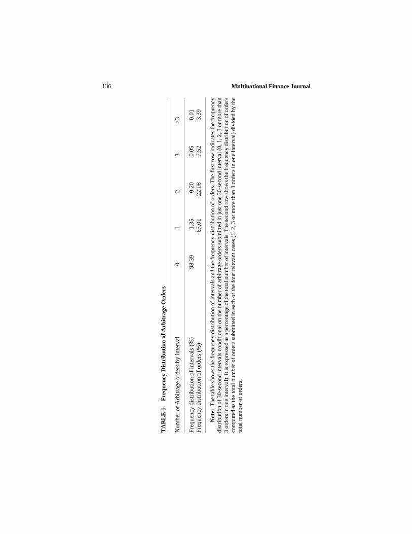
Time series with the recorded program trades expressed in units often millions of French francs as a variable are set up. The length of eachinterval of time is fixed at 30 seconds, that is, orders are aggregatedwith respect to this time scale. When no arbitrage order occurs then thevariable takes the value of zero. The independence of the submissionsis then characterized by the distribution of orders per interval and by atransition matrix. The distribution of orders is presented in table 1.

The first row in table 1 shows the frequency distribution of30-second intervals conditional on the number of arbitrage ordersubmitted in just one 30-second interval and is expressed as apercentage of the total number of intervals. It appears that arbitrageurstrade very infrequently. The number of 30-second intervals concernedwith arbitrage orders represents less than 2% of the total number ofperiods. Furthermore, arbitrage order submissions appear to be highlyconcentrated. The second row of the table shows the frequencydistribution of arbitrage orders. In one third of the cases, there are morethan one order submission per period of 30 seconds. This clusteringeffect is reinforced by the autocorrelation of the order submission assuggested by the conditional probabilities of the transition matrixpresented in table 2.

The conditional probability that a buy (sell) order follows anotherbuy (sell) order appears significantly greater than the unconditionalprobability of a buy(sell) order occurrence. This phenomenon indicatesthat basket orders of a same side of the market arrive in clusters. Thisevidence is consistent with the related findings of Harris, Sofianos andShapiro (1994) for the U.S. market. It suggests that more than one orderis needed to induce mean revertion in basis changes but also thatarbitrageurs react roughly simultaneously in some “jumping the gun”competition, as analyzed for example by Spatt and Sterbenz (1985).Nevertheless, results of Biais, Hillion and Spatt (1995) suggest that thisorder flow autocorrelation does not characterize the arbitrage order flowspecifically.

One can expect that on average the cash and carry arbitrage(associated with buy basket orders) is related to a positive mispricing


TA

BL

E 1

.F

requ

ency

Dis

trib

utio

n of

Arb

itra

ge O

rder

s

Num

ber

of A

rbit

rage

ord

ers

by in

terv

al0

12

3>

3

Fre

quen

cy d

istr

ibut

ion

of in

terv

als

(%)

98.3

91.

350.

200.

050.

01F

requ

ency

dis

trib

utio

n of

ord

ers

(%)

67.0

122

.08

7.52

3.39

Not

e: T

he ta

ble

show

s th

e fr

eque

ncy

dist

ribu

tion

of

inte

rval

s an

d th

e fr

eque

ncy

dist

ribu

tion

of

orde

rs. T

he f

irst

row

indi

cate

s th

e fr

eque

ncy

dist

ribu

tion

of

30-s

econ

d in

terv

als

cond

itio

nal o

n th

e nu

mbe

r of

arb

itra

ge o

rder

s su

bmit

ted

in ju

st o

ne 3

0-se

cond

inte

rval

(0,

1, 2

, 3 o

r m

ore

than

3 or

ders

in o

ne in

terv

al).

It is

exp

ress

ed a

s a

perc

enta

ge o

f the

tota

l num

ber o

f int

erva

ls. T

he s

econ

d ro

w s

how

s th

e fr

eque

ncy

dist

ribu

tion

of o

rder

sco

mpu

ted

as th

e to

tal n

umbe

r of

ord

ers

subm

itte

d in

eac

h of

the

four

rel

evan

t cas

es (

1, 2

, 3 o

r m

ore

than

3 o

rder

s in

one

inte

rval

) di

vide

d by

the

tota

l num

ber

of o

rder

s.


TA

BL

E 2

.T

rans

itio

n M

atri

x fo

r A

rbit

rage

Ord

er S

ubm

issi

ons

tN

o or

der

Buy

ord

erS

ell o

rder

No

orde

r96

.76

82.7

580

.52

t + 1

Buy

Ord

er1.

4915

.31

1.40

Sel

l Ord

er1.

811.

9418

.08

Sum

100.

0010

0.00

100.

00

Not

e: T

he tr

ansi

tion

mat

rix

give

s th

e pr

obab

ilit

y th

at a

n ev

ent o

f ty

pe j

occu

rs a

t tim

e t +

1 g

iven

a s

peci

fic

even

t occ

urre

d at

tim

e t.

Thu

s th

em

atri

x sh

ould

be

read

by

colu

mn.

Typ

es j

refe

r to

the

abse

nce

of a

rbit

rage

ord

er s

ubm

issi

on, t

o th

e bu

y ar

bitr

age

orde

r su

bmis

sion

and

to th

e se

llar

bitr

age

orde

r su

bmis

sion

. Tim

e t r

efer

s to

30-

seco

nd in

terv

als.

Mul

tipl

e or

der

subm

issi

ons

occu

rrin

g in

the

sam

e in

terv

al h

ave

been

cou

nted

for

the

net o

rder

type

(e.

g. o

ne b

uy o

rder

and

two

sell

ord

ers

acco

unt f

or a

sel

l ord

er)

or h

ave

been

oth

erw

ise

igno

red

(e.g

. one

buy

ord

er a

nd o

ne s

ell

orde

r ac

coun

t for

the

abse

nce

of o

rder

sub

mis

sion

).


TA

BL

E 3

.B

aske

t T

radi

ng, M

ispr

icin

g an

d L

iqui

dity

Buy

Sel

lB

uy a

nd S

ell

Tot

alM

is>

0M

is<

0

# O

bs.

675

852

1527

5002

016

414

3360

6M

is0.

0869

–0.1

831

–0.0

637

–0.0

435

0.05

32–0

.090

7(0

.092

4)(0

.098

6)(0

.164

9)(0

.092

5)(0

.041

1)(0

.071

6)θ

0.65

250.

1500

0.37

740.

4226

0.63

010.

3213

(0.2

387)

(0.2

483)

(0.3

457)

(0.2

288)

(0.1

364)

(0.1

937)

θ$1

3333

111

θ#0

170

170

1788

θ$0.

6536

19

370

7379

θ#0.

1517

377

394

5042

Spr

ead

0.24

570.

2517

0.24

900.

2511

0.24

630.

2534

(0.0

651)

(0.0

612)

(0.0

630)

(0.0

515)

(0.0

503)

(0.0

519)

Dep

th20

79.5

919

25.6

619

93.7

018

69.7

719

15.3

718

47.5

0(7

39.6

1)(5

90.5

6)(6

64.7

9)(5

84.9

1)(6

55.2

4)(5

45.9

1)

Not

e: T

he s

tati

stic

s gi

ven

in th

e ta

ble

are

cond

itio

nal o

n bu

y or

ders

, sel

l ord

ers,

buy

and

sel

l ord

ers,

pos

itiv

e an

d ne

gati

ve m

ispr

icin

g va

lues

and

are

also

giv

en f

or th

e fu

ll s

ampl

e. T

he b

id-a

sk s

prea

d an

d th

e de

pth

are

com

pute

d fr

om th

e la

st q

uote

s an

d th

e de

pth

avai

labl

e at

thes

e qu

otes

for

each

sto

ck a

t the

end

of

each

30-

seco

nd in

terv

al. S

tand

ard

erro

rs a

re g

iven

in p

aren

thes

es.


value and that on average the reverse arbitrage (associated with sellbasket orders) are related to a negative mispricing value. The resultspresented in table 3 show that it is actually the case.

The first row of table 3 gives the number of events considered. Asa result of the clustering effect noted above, the number of arbitrageevents that appears here is slightly lower than previously stated becauseorders are aggregated with respect to 30-second intervals. Over thesample period the futures more often appears underpriced (67.2 percentof the time) than overpriced which is consistent with the asymmetryobserved between the number of cash and carry and reverse cash andcarry trades.

The average mispricing value is reported in the second row of thetable conditional on a cash and carry event, a reverse cash and carryevent, an arbitrage trading event and for the full sample. The averagevalues for the positive and negative mispricings are also provided. Itappears that on average cash and carry (reverse cash and carry)arbitrages are associated with a positive (negative) value of themispricing, which is consistent with the traditional cost of carryargument.

Nevertheless these average bounds are not symmetrically distributedaround the theoretical futures value. The absolute value of the averagemispricing for reverse cash and carry arbitrages is about twice as largeas the value of the average mispricing for cash and carry trades. Thisasymmetry also appears in the average value of the mispricing computedfor the full sample and indicates that the value of the futures computedfrom the cost of carry formula may be systematically too large.Therefore it may be the case that the asymmetry observed in thearbitrage bound just reflects the undervaluation of the futures relativeto the theoretical price we computed. Finally it appears that the discountrelative to the cost of carry price is small with an average value of 0.043percent of the index where the average bid-ask spread on a portfolio thatduplicates the index equals 0.25 percent of the index over the period.

The average value of θ is displayed in the third row of the table. Themean value computed from the total sample (0.4226) indicates that theactual futures value is lower than the average value of the theoreticalfutures computed with the bid and ask stock quotes and confirms theprevious finding. More importantly, the mean value of the variable θassociated with cash and carry (say θbuy) or reverse cash and carry (sayθsell) arbitrages suggests that the size of the mispricing that triggersarbitrage is significantly reduced vis-à-vis the size of the mispricing


13. Unfortunately we cannot provide statistics based on a distinction between theestablishing and liquidating trades because our database provides no information on such adistinction. Nevertheless in the next section we test for the influence of variables that may berelated to the early liquidation option model.

FIGURE 1.—Theta against Time-to-Maturity — January 1995 ContractThis figure displays the variable theta against time-to-maturity for theJanuary 1995 contract. Observations on the same day form vertical linesand days are counted to maturity.

associated with “simple arbitrage opportunity” (Brennan and Schwartz[1990]), that is mispricing associated with arbitrage position held untilmaturity. The reported means are 0.6525 and 0.1500 for θbuy and θsell,respectively. Corresponding “simple arbitrage opportunity” boundswould have been 1 and 0 for θbuy and θsell, respectively.

This finding is consistent with the early liquidation option model ofBrennan and Schwartz (1990) — establishing an arbitrage position canbe viewed as making the arbitrage and simultaneously acquiring anoption to unwind the position when there are arbitrage profits fromunwinding it — and is in accordance with previous empirical evidenceprovided by Sofianos (1993) and Neal (1996) for the U.S. market.13

Finally, we note that θbuy – θsell = 0.5, which is exactly what onecould expect theoretically if arbitrageur were 100% certain of beingable to unwind their position prior to the maturity date and competitionamong arbitrageur had eliminated all excess rents. That is, if the grossprofit is half the spread when establishing a position plus half the spread

-0,5

0

0,5

1

1,5

0 5 10 15 20

Time-to-maturity

θ


14. We thanks an anonymous referee for pointing out this fact.

FIGURE 2.— Theta against Time-to-Maturity —February 1995 ContractThis figure displays the variable theta against time-to-maturity forFebruary 1995 contract. Observations on the same day form verticallines and days are counted to maturity.

when unwinding the position (with certainty), then the net arbitrageprofit is at the competitive-level of zero.14

In this context, it would be interesting to gauge how frequently andconsistently one is able to unwind a position early. With this in mind,we made simple plots of the evolution of θ against time-to-maturity foreach of the 3 contracts maturing during our sample period. These plotsare very similar to the plots A1-A16 in Brennan and Schwartz (1990)and are presented in figures 1 to 3. Observations on the same day formvertical lines and days are counted down to maturity.

As discussed in Brennan and Schwartz (1980), maximum arbitrageprofit are realized when θ passes from one extremum to another.Assuming that no arbitrage is possible inside a band equal to one halfof the spread, it seems that the intra-day evolution of θ makes it possiblefor arbitrageur to trade in cash and carry and in reverse cash and carryeach day, and that for the most part of the days of the sample. Thereforeit may be the case that arbitrageurs can enter into new positions or closeexisting ones almost each day, trading mainly on a daily basis.However, the 2-dimensional view of these plots may be misleading,

-0,5

0

0,5

1

1,5

0 5 10 15 20

Time-to-maturity

θ


FIGURE 3.— Theta against Time-to-Maturity — March 1995 ContractThis figure displays the variable theta against time-to-maturity for theMarch 1995 contract. Observations on the same day form vertical linesand days are counted to maturity.

making us to overestimate the weight of larger and smaller observations.Figure 4 presents a simple histogram of the observations againsttime-to-maturity and shows that the observations are indeed much lessdispersed. This figure also suggests possible time-variation in the meanvalue of θ. The analysis of some possible trigger points deserve furthercomments.

Consider first the trigger points associated with the ”establish andhold to maturity” arbitrage. The number of arbitrage orders submittedwhen the mispricing exceeds the bounds θ = 1 or θ = 0 appears limited,about 13.3 percent of all arbitrage trades as shown in rows 4 and 5 oftable 3. In other words, arbitrageurs expect most of the time to unwindtheir position before maturity and price the futures accordingly.However, if the futures becomes too cheap/expensive vis-à-vis thestocks, then they trade heavily. For example, while the futures appearsoverpriced less than 1 hour over the 3 month covered in the study (111observations of 30-second intervals, that is 0.22 percent of the calendartime analyzed), it concentrates during that 1-hour period more than 2percent of the arbitrage orders. One should also note that the number ofviolations is also limited, representing less than 3.8 percent of the

-1,5

-1

-0,5

0

0,5

1

1,5

2

0 5 10 15 20

Time-to-maturity

π


FIGURE 4.— Mispricing Distribution This figure displays the distribution of mispricing againsttime-to-maturity for the period from January 1995 through March 1995.Data are aggregated by increments of theta of 0.1.

number of intervals, this percentage being probably overestimated dueto the small undervaluation of the futures we discussed previously. Allin all, this suggests that on average the futures is well priced, but alsothat arbitrage trading will be difficult to predict with the traditional costof carry argument alone.

Consider now the trigger points associated with competitivearbitrageurs trading in anticipation of (nearly always) unwinding early.These are obtained by adding and subtracting on-quarter of the spreadto the average mispricing which is about θ = 0.4, yielding to triggerspoints θbuy and θsell equal to 0.65 and 0.15, respectively. Note that thesetrigger points are exactly what we see on average, i.e. the mean valuereported in the third row of the table and discussed previously. Thenumber of buy(sell) arbitrage orders above(below) these points arereported in table 3, raws 6 and 7. As expected, a large proportion ofarbitrage orders are submitted at and above the value θbuy = 0.65 and atand below θsell = 0.15. The reported evidence indicates that 50 percentof the arbitrage orders are concentrated on 25 percent of the tradingtime. However, this also means that about 50 percent of arbitragetrading is still not well explained. Figures 5 and 6 provide a moreprecise picture of when arbitrage positions are established. Each

1

6

1 1

1 6

2 1

<0

0-0

.1

0.1

-0.2

0.2

-0.3

0.3

-0.4

0.4

-0.5

0.5

-0.6

0.6

-0.7

0.7

-0.8

0.8

-0.9

0.9

-1

>1

0

0 , 2

0 , 4

0 , 6

0 , 8

1

1 , 2

O b s . (% )

T im e - to -m a tu rity

T he ta


FIGURE 5.— Cash and Carry Arbitrage DistributionThis figure displays the distribution of cash and carry arbitrage againsttime-to-maturity for the period from January 1995 through March 1995.Arbitrage data are aggregated by increments of theta of 0.1.

histogram reports the repartition of the arbitrage trades by 0.1increments of θ.

These figures confirm that there is still a lot of dispersion around thetriggers points θbuy = 0.65 and θsell = 0.15. Furthermore, they show thatthere is some time-variation in the trigger points. One possible reasonfor these behaviors may be found in an argument initially developed byKawaller (1991). She argues that “no single break-even price isuniversally appropriate, but rather that the break-even price for a giveninstitution depends on the motivation of that firm as well as on itsmarginal funding and investing yield alternatives”(Kawaller [1991, p.453]). The threshold models developed by Tse (2001), Yadav and Pope(2000) and Dwyer, Locke and Yu (1996) are built on the samehypothesis of heterogeneous arbitrage.

The bid-ask spread associated with buy and sell orders is notsignificantly different from its full sample mean (t-stat for the differenceequals –1.2437). Accordingly, it suggests that there is no systematicpattern in the arbitrage bounds associated with arbitrage orders thatwould be related to variations in the bid-ask spread. Put another way, itmeans that arbitrage trading is not related to large mispricing valuesinduced by some liquidity shocks affecting the bid-ask spread in thestock market.

Nevertheless, the data indicate that a liquidity pattern is found in the

1

5

9

1 3

1 7

2 1

< - 0 . 4

( 0 .3 ) - ( 0 .2 )

( 0 . 1 ) - 0

0 . 1 - 0 . 2

0 .3 - 0 .4

0 .5 - 0 . 6

0 .7 - 0 .8

0 .9 - 1

1 .1 - 1 . 2

0

1

2

3

4

O bs . (% )

T im e - to -m a tu r ityT he ta


15. The same computation for the spread gives the value of 0.273 percent and 0.268percent for the sub- sample and for the orders over this sub-sample, respectively, with a t-statfor the difference of 2.01.

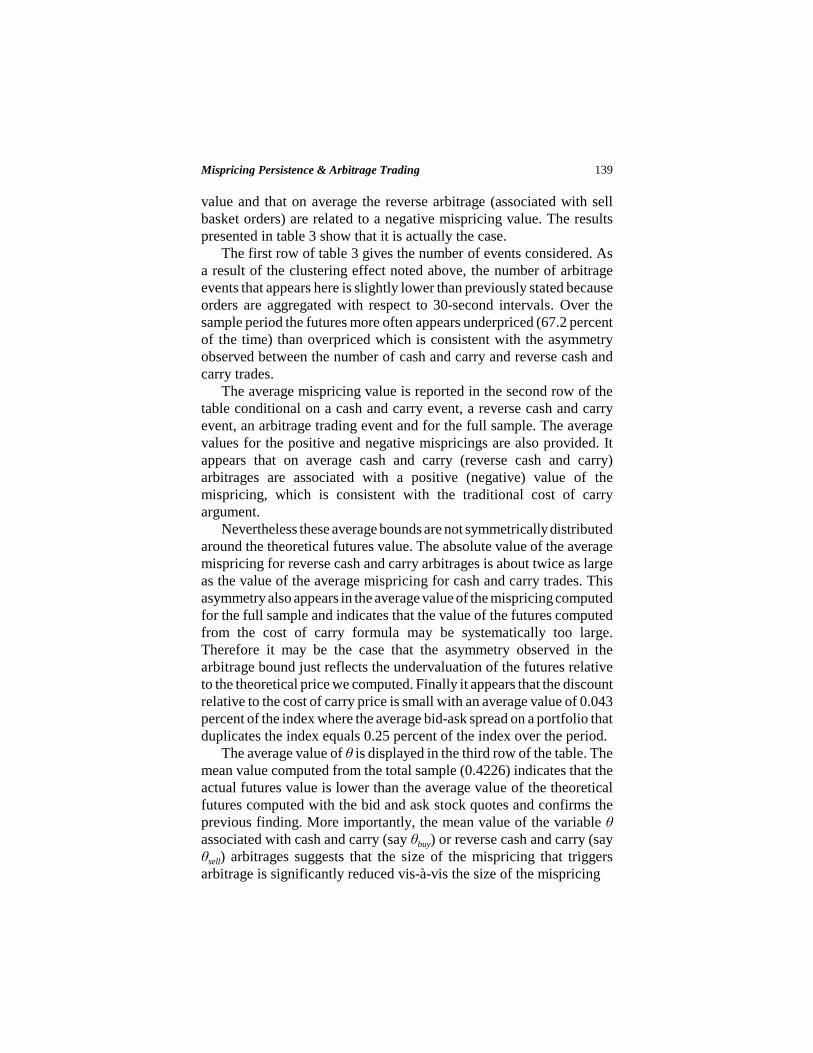
FIGURE 6. — Reverse Cash and Carry Arbitrage DistributionThis figure displays the distribution of reverse cash and carry arbitrageagainst and time-to-maturity for the period from January 1995 throughMarch 1995. Arbitrage data are aggregated by increments of theta of0.1.

number of shares available at the best quotes (i.e., the depth). At thetime of arbitrage trading the depth at the best quotes appearssignificantly larger than the average depth (t-stat for the differenceequals 7.20). This suggests that the submission of arbitrage orders maysometimes be constrained by a lack of liquidity in the market.Furthermore, it suggests that some mispricing persistence may beinduced by this lack of liquidity.

In order to illustrate this point further, we computed the averagedepth over the sub-sample where all mispricing values inside sometransaction bounds were discarded and compared it to the average depthcorresponding to arbitrage orders submitted in this sub-sample of data.Taking for example the average mispricing values associated with buyand sell orders as some (arbitrary) transaction bounds, we find that theaverage depth over the sub-sample is equal to 1880.89 shares where theaverage depth associated with buy and sell orders over the sub-sampleequals 1983.66 shares with a t-stat for the difference of 4.10 and highlysignificant.15

1

5

9

1 3

1 7

2 1

<-0.

4

(0.3

)-(0

.2)

(0.1

)-0

0.1-

0.2

0.3-

0.4

0.5

-0.6

0.7-

0.8

0.9-

1

1.1-

1.2

0

1

2

3

4

O b s . ( % )

T im e - to - m a tu r it y

T h e t a


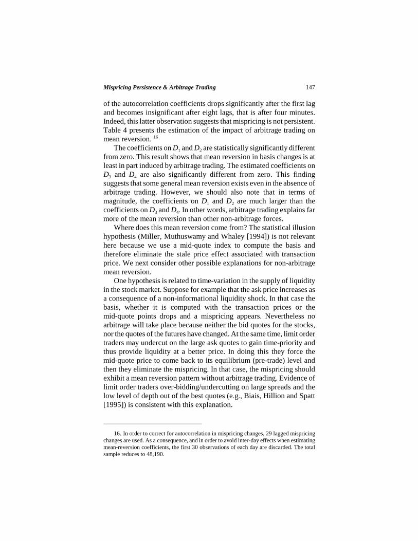
FIGURE 7. — Basis Changes Autocorrelation FunctionThis figure displays the autocorrelation function of the CAC40 basischanges for the period from January 1995 through March 1995. Data aresampled on 30-second intervals. Confidence intervals of +/- 2 standarddeviations (Bartlett formula) are also reported to test the null hypothesisof zero autocorrelation.

This is consistent with the view that arbitrage is not undertakenwhen the supply of liquidity appears too low, even when the mispricingvalue exceeds some thresholds. We present a test of this hypothesis inthe next section.

V. Regression Results

Before we turn to the estimates of the regressions, we consider theautocorrelation function of the mispricing changes series. Thisautocorrelation function is of interest because first and higher orders ofautocorrelation coefficients show the persistence of mispricing (e.g.,Mackinlay and Ramaswamy [1988]). The estimated autocorrrelationfunction is presented in figure 7.

We note that the mispricing changes series exhibit significantnegative autocorrelation which is in accordance with the mean revertingbehavior one could expect for the basis. We also observe that the value

-0,14

-0,12

-0,1

-0,08

-0,06

-0,04

-0,02

0

0,02

0 1 2 3 4 5 6 7 8 9 10 11 12 13 14 15 16 17 18 19 20

Lag

Aut

ocor

rela

tion


16. In order to correct for autocorrelation in mispricing changes, 29 lagged mispricingchanges are used. As a consequence, and in order to avoid inter-day effects when estimatingmean-reversion coefficients, the first 30 observations of each day are discarded. The totalsample reduces to 48,190.

of the autocorrelation coefficients drops significantly after the first lagand becomes insignificant after eight lags, that is after four minutes.Indeed, this latter observation suggests that mispricing is not persistent.Table 4 presents the estimation of the impact of arbitrage trading onmean reversion. 16

The coefficients on D1 and D2 are statistically significantly differentfrom zero. This result shows that mean reversion in basis changes is atleast in part induced by arbitrage trading. The estimated coefficients onD3 and D4 are also significantly different from zero. This findingsuggests that some general mean reversion exists even in the absence ofarbitrage trading. However, we should also note that in terms ofmagnitude, the coefficients on D1 and D2 are much larger than thecoefficients on D3 and D4. In other words, arbitrage trading explains farmore of the mean reversion than other non-arbitrage forces.

Where does this mean reversion come from? The statistical illusionhypothesis (Miller, Muthuswamy and Whaley [1994]) is not relevanthere because we use a mid-quote index to compute the basis andtherefore eliminate the stale price effect associated with transactionprice. We next consider other possible explanations for non-arbitragemean reversion.

One hypothesis is related to time-variation in the supply of liquidityin the stock market. Suppose for example that the ask price increases asa consequence of a non-informational liquidity shock. In that case thebasis, whether it is computed with the transaction prices or themid-quote points drops and a mispricing appears. Nevertheless noarbitrage will take place because neither the bid quotes for the stocks,nor the quotes of the futures have changed. At the same time, limit ordertraders may undercut on the large ask quotes to gain time-priority andthus provide liquidity at a better price. In doing this they force themid-quote price to come back to its equilibrium (pre-trade) level andthen they eliminate the mispricing. In that case, the mispricing shouldexhibit a mean reversion pattern without arbitrage trading. Evidence oflimit order traders over-bidding/undercutting on large spreads and thelow level of depth out of the best quotes (e.g., Biais, Hillion and Spatt[1995]) is consistent with this explanation.


17. Additional results available upon request indicate that the index return dynamics isbest modeled as an ARMA(2,1).

18. We thanks an anonymous referee for pointing out this explanation.

TABLE 4. Mean Reversion and Arbitrage Trading

α TTM D1 D2 D3 D4

Coefficient 0.0008 –0.0001 –0.2754 –0.1412 –0.0761 –0.0163t–stat (1.87) (–2.11) (–22.14) (–21.95) (–12.17) (–5.5986)

# Obs. = 48160 R2 = 0.0865 Q(36) = 42.3443

Note: This table contains the results of the mean reversion equation for the mispricing:

4

11 1

p

t t i i t i t j ti j

MIS TTM D MIS MISα β γ φ ε− −= =

Δ = + + + Δ +∑ ∑where TTM denotes the time-to-maturity in days, MIS is the value of the mispricing and ΔMISis the first difference in MIS. If a long arbitrage position is established at time t then D1 = 1and if a short arbitrage position is established then D2 = 1. If there is no arbitrage trading attime t then D3 = 1 for positive mispricing and D4 = 1 for negative mispricing. Whenever thedummies are not equal to 1, they are zero.

Thus, it may be the case that this liquidity effect results in a bid-askbounce effect which in turn produces a moving average component inthe index dynamics (e.g., Stoll and Whaley [1990]).17 Then, followingMiller, Muthuswamy and Whaley (1994), we conjecture that theliquidity effect induces at least some part of the negative autocorrelationin mispricing changes. Finally, the observed mean reversion due to aliquidity shock must be economically small and the results support that.

An alternative explanation for non-arbitrage mean reversion relieson the lead-lag relationships between the futures and the stocks.18 It ispossible that new information is impounded in one market first (saystock index futures), causing an increase in mispricing, and then tradersobserve the change in futures price, and make corresponding changes inlimit order (by canceling and resubmitting at new limit order prices) inthe underlying stocks, which decreases mispricing. Thus, one wouldnaturally expect some mean reversion to take place without arbitragetrading. Evidence of stale quotes, not prices, in the cash market isconsistent with this hypothesis. The first order autocorrelation for themid-quote index return series is 0.184 and is significantly different fromzero.


19. It is not clear whether the explanatory variables should be measured at time t or attime t – 1. Fortunately the results are not affected by this choice and we decided to report theresults based on variables measured at time t.

Finally, one can also consider the partial adjustment model ofTheobald and Yallup (2001) and the information dissemination modelof Chan (1993) as possible candidates. These models propose rationalesfor stale prices and index autocorrelation that differ from the infrequenttrading hypothesis.

The results concerning the determinants of arbitrage trading arepresented in table 5.19

The results indicate that the probability for an arbitrageur to trade ispositively associated with the size of the price discrepancy but also thatthis size effect is more pronounced for negative mispricing. This resultis in accordance with the descriptive statistics presented above and withnumerous papers that indicate that arbitrage bounds are notsymmetrically distributed around the theoretical futures price. This isconsistent with the cost and uncertainty that characterize short sales inreverse arbitrage.

As suggested previously the results show that arbitrageurs take intoaccount the depth of the market when establishing a position.Furthermore, it seems that arbitrageurs also focus on the bid-ask spread.This latter result is probably induced by the larger mispricings for whichthe size of the spread matters.

The negative and significant coefficient for the DURATION variableis puzzling because our hypothesis was that the longer the futures stayedover-priced or under-priced, the higher would be the probability for anarbitrageur to establish a position. This is in fact not the case, perhapsbecause the futures may stay over-priced or under-priced for a longperiod of time but at a level that makes arbitrage unattractive. We mayalso consider that arbitrage trading reduces large mispricings but doesnot eliminate them instantaneously. In order to take into account thesepossibilities we re-estimated the model with the DURATION variabledefined over various threshold but the estimated coefficient of thevariable DURATION was still negative and significant. We also plottedthe average value of the cumulative changes in the mispricing valuefrom 10 minutes before the trade to 10 minutes after the trade. Theresulting pattern for cash and carry and reverse cash and carry arbitragesis presented in figure 8.

Inspection of the figure indicates that on average mispricing rises


TA

BL

E 5

.A

Log

it M

odel

of

Arb

itra

ge T

radi

ng

Cst

.A

BSM

ISN

EG

MIS

DU

RA

TIO

NSP

RE

AD

DE

PT

HR

EV

ER

SAL

TT

MA

OIM

B

–5.0

225

13.1

703

2.61

13–0

.019

2–0

.263

90.

0008

1.91

700.

0179

–0.1

189

(–15

.71)

(23.

13)

(4.8

1)(–

8.79

)(–

8.48

)(1

3.72

)(3

.52)

(3.6

6)(–

1.99

)

Not

e: T

he ta

ble

show

s th

e es

tim

ated

coe

ffic

ient

s ob

tain

ed f

rom

a lo

git m

odel

of

arbi

trag

e tr

adin

g. T

he d

epen

dant

var

iabl

e is

1 if

an

arbi

trag

epo

siti

on is

est

abli

shed

at t

ime

t and

zer

o ot

herw

ise.

The

con

diti

onal

var

iabl

es a

re a

s fo

llow

s: A

BSM

IS is

the

abso

lute

val

ue o

f th

e m

ispr

icin

g an

dN

EG

MIS

take

s th

e va

lue

of 1

for n

egat

ive

mis

pric

ing

and

0 ot

herw

ise.

DU

RA

TIO

N is

def

ined

as

the

dura

tion

of a

giv

en m

ispr

icin

g ev

ent c

ondi

tion

alon

the

theo

reti

cal f

utur

es p

rice

. SP

RE

AD

is th

e w

eigh

ted

aver

age

bid-

ask

spre

ad o

f the

40

inde

x st

ocks

and

DE

PT

H is

the

wei

ghte

d av

erag

e nu

mbe

rof

sha

res

avai

labl

e at

the

best

quo

te o

n th

e si

de o

f the

mar

ket a

ssoc

iate

d w

ith

the

mis

pric

ing

sign

. RE

VE

RSA

L is

the

perc

enta

ge o

f rev

erse

mis

pric

ing

over

the

next

sev

en tr

adin

g ho

urs.

TT

M is

the

tim

e-to

-mat

urit

y. A

OIM

B ta

kes

the

valu

e of

1, i

f the

arb

itra

ge th

at w

ould

be

asso

ciat

ed w

ith

the

curr

ent

mis

pric

ing

valu

e re

duce

s th

e ar

bitr

age

orde

r im

bala

nce

resu

ltin

g fr

om p

revi

ous

arbi

trag

e tr

ades

, and

0 o

ther

wis

e.


FIGURE 8.— Cumulative Basis Changes around Arbitrage TradingThis figure displays the behavior of the basis surrounding buy and sellbasket order submissions for the period from January 1995 throughMarch 1995. The estimates plotted are obtained from time seriesregressions of the basis changes on leads and lags of buy and sell ordersubmissions. This procedure is taken from Harris, Sofianos and Shapiro(1994) and allows us to account for the clustering effect observed inarbitrage order submissions.

sharply just one or two minutes before the order submission and thendrops quickly after the arbitrage trade is completed. This provides directevidence on the mean reversion induced by arbitrage trading and alsoindicates that the mispricing is not persistent around such events. Itsuggests that true arbitrage opportunities may be due to sudden pricejumps induced by information arrivals that are quicky exploited by thearbitrageurs. This is consistent with models of informed arbitragetrading (e.g., Kumar and Seppi [1994]) and with the evidence that thefutures price leads the index price around arbitrage trading. Figures 9and 10 below present the plots of the cumulative changes in the indexcash and futures value from 10 minutes before the trade to 10 minutesafter the trade for cash and carry and reverse arbitrages.

The variables related to the option to liquidate the position earlysupport the hypothesis that this option is of some value for arbitrageurs.The likelihood of establishing an arbitrage position is a positive

- 0 ,0 5

- 0 ,0 4

- 0 ,0 3

- 0 ,0 2

- 0 ,0 1

0

0 ,0 1

0 ,0 2

0 ,0 3

0 ,0 4

- 1 0 - 8 - 6 - 4 - 2 0 2 4 6 8 1 0

E ve n t t im e in m in u t e s

Evo

lutio

n of

the

bas

is (

in %

)

C a s h a n d c a r r ya r b itr a g eR e v e r s e a r b itr a g e


FIGURE 9.— The Price Impact of Cash and Carry ArbitrageThis figure displays the cumulative returns of the mid-quote index andthe cumulative price changes of the futures surrounding buy basketorder submissions for the period from January 1995 through March1995. The estimates plotted are obtained from time series regressions ofthe basis changes on leads and lags of buy and sell order submissions.This procedure is taken from Harris, Sofianos and Shapiro (1994) andallows us to account for the clustering effect observed in arbitrage ordersubmissions.

function of the expected reversal in the basis indicating that arbitrageurstake into account the possibility to liquidate a position early when theyare looking for arbitrage opportunities. The positive coefficient for thetime to maturity is also consistent with arbitrageurs valuing the optionto reverse their positions early. Curiously, arbitrage order imbalance hasan impact on the likelihood of establishing a new arbitrage positionopposite to the one we expected. Nevertheless the joint effect of a largenumber of data and a low critical value may indicate that arbitrage orderimbalance has in fact no impact on the likelihood of establishing anarbitrage position. These results are consistent with the fact thatarbitrageurs are forward-looking when establishing a position (assuggested by the coefficient of the REVERSAL variable), notbackward-looking.

- 0 ,0 1

0

0 ,0 1

0 ,0 2

0 ,0 3

0 ,0 4

0 ,0 5

0 ,0 6

- 1 0 0 1 0 2 0 3 0E ven t t im e in m in u tes

Cum

ulat

ed r

etur

ns (

in%

)

Fu tu r e s M id - q u o te in d e x


20. Neal (1996), page 558, finds a value of 0.03.

FIGURE 10.— The Price Impact of Reverse Cash and Carry ArbitrageThis figure displays the cumulative returns of the mid-quote index andthe cumulative price changes of the futures surrounding buy basketorder submissions for the period from January 1995 through March1995. The estimates plotted are obtained from time series regressions ofthe basis changes on leads and lags of buy and sell order submissions.This procedure is taken from Harris, Sofianos and Shapiro (1994) andallows us to account for the clustering effect observed in arbitrage ordersubmissions.

Finally, while the model provides new results concerning thedeterminants of arbitrage trading, its ability to predict when an arbitrageposition will be established is very low. The likelihood ratio indexequals 0.088 and the R-squared from a similar OLS regression equals0.058. This is significantly better than the goodness of fit statisticsreported in previous studies, a fact probably due to the new variablesincluded in the model, but it is still very low.20 This suggests that whilethe liquidity of the market and the opportunity to reverse a position areimportant determinants in the arbitrage decision, a great deal ofheterogeneity among arbitrageurs still remains. It also suggests that theactual mechanism of arbitrage trading may be far more complex thancaptured by the traditional threshold models.

- 0 ,0 8

- 0 ,0 7

- 0 ,0 6

- 0 ,0 5

- 0 ,0 4

- 0 ,0 3

- 0 ,0 2

- 0 ,0 1

0

- 1 0 0 1 0 2 0 3 0E ve n t t im e in m in u t e s

Cum

ulat

ed r

etur

ns (

in %

)

F u tu r e s M id - q u o te in d e x


VI. Summary and Conclusions

This paper focuses on the behavior of arbitrageurs in stock index cashand futures markets. Relying on a dataset of intra-day arbitrage ordersin the French market, the persistence of mispricing and the arbitragetrading decision are analyzed.

Controlling for the statistical illusion induced by infrequent trading,we show that mispricing is not persistent because arbitrageopportunities are rapidly eliminated by stock index arbitrageurs but alsobecause of some general mean reversion in mispricing changes.

We suggest that this result, which is reminiscent to the work byMiller, Muthuswamy and Whaley (1994), may be related to the fact thatarbitrage trading is far less frequent and predictable that it would befound by applying some mechanical trading rules based on themispricing value.

We suggest that the non-arbitrage mean reversion may be related tothe behavior of limit order traders facing liquidity shocks and also tostale quotes in the cash market. The first explanation is consistent withevidence of limit order traders over-bidding/undercutting on largespreads and also with the low level of depth out of the best quotes (e.g.Biais, Hillion and Spatt [1995]). The second explanation may be relatedto lead-lag relationships between the futures and the stocks and is alsoconsistent with the partial adjustment model of Theobald and Yallup(2001).

In this context, the behavior of arbitrageurs appears highlycompetitive. The results are consistent with what one would expecttheoretically if arbitrageurs were 100% certain being able to unwindtheir position prior to the maturity date and competition amongarbitrageurs had eliminated all excess rents. That is, we find that onaverage the net arbitrage profit is at the competitive level of zero.Finally we show that the depth of the market affect significantlyarbitrage trading.

Additional research is needed to increase our ability to predict whenan arbitrage position is established. Future work may examine the extentto which arbitrageurs act as an homogeneous set of investors usingactual arbitrage data. In the same vein, the aggressiveness of arbitragetrading may be analyzed.


References

Biais, B.; Hillion, P.; and Spatt, C. 1995. An empirical analysis of the limitorder book in the Paris Bourse. Journal of Finance 50 (December):1655–1689.

Brennan, M., and Schwartz, E. 1990. Arbitrage in stock index futures. Journalof Business 3 (January): S7–S31.

Chan, K. 1993. Imperfect information and cross-autocorrelation among stockprices. Journal of Finance 48 (September): 1211–1230.

Cheung, Y.-W., and Fung, H.-G. 1997. Information flows between Eurodollarspot and futures markets. Multinational Journal of Finance 1 (December):255–271.

Chung, Y.P. 1991. A transaction data test of stock index futures marketefficiency and index arbitrage efficiency. Journal of Finance 46(December): 1791–1809.

Dwyer, G.P. Jr; Locke P.; and Yu W. 1996. Index arbitrage and nonlineardynamics between the S&P 500 futures and cash. Review of FinancialStudies 9 (Spring): 301–332.

Fremault, A. 1991. Index futures and index arbitrage in a rational expectationmodel. Journal of Business 64 (October): 523–548.

Froot, K.A., and Pérold A.F. 1995. New trading practices and short-run marketefficiency. Journal of Futures Markets 15 (October): 731–765.

Harris, L.; Sofianos, G.; and Shapiro J.E. 1994. Program trading and intradayvolatility. Review of Financial Studies 7 (Winter): 653–685.

Holden, C.W. 1995. Index arbitrage as cross-sectional market making. Journalof Futures Markets 15 (June): 423–455.

Holden, C.W. 1990. Intertemporal arbitrage trading : theory and empirical tests.Working Paper. Indiana University.

Kawaller, I.G. 1991. Determining the relevant fair value(s) of the S&P 500futures: A case study approach. Journal of Futures Markets 11 (August):423–455.

Kempf, A. 1998. Short selling, unwinding, and mispricing. Journal of FuturesMarket 18 (December): 903–923.

Kraus, A., and Stoll, H.R. 1972. Price impacts of block trading on the NewYork Stock Exchange. Journal of Finance 27 (June): 569–588.

Kumar, P., and Seppi, D. 1994. Information and index arbitrage. Journal ofBusiness 67 (October): 481–509.

Lambrecht, B. 2000. The timing of arbitrage: An options approach. Finance 21(December):131–167.

Lim, K.-G. 1992. Arbitrage and price behavior of Nikkei stock index futures.Journal of Futures Markets 12 (April): 151–161.

MacKinlay, A.C., and Ramaswamy, K. 1988. Index-futures arbitrage and thebehavior of stock index futures prices. Review of Financial Studies 1(Summer): 137–158.


McDonald, R.L. 2001. Cross-border investing with tax arbitrage : The case ofGerman tax credits. Review of Financial Studies 14 (Fall): 617–657.

Miller, M.H.; Muthuswamy, J.; and Whaley, R.E. 1994. Mean reversion of S&P500 index basis changes: Arbitrage induced or statistical illusion? Journalof Finance 49 (June): 479–513.

Neal, R. 1996. Direct tests of index arbitrage models. Journal of Financial andQuantitative Analysis 31 (December): 541–562.

Sofianos, G. 1993. Index arbitrage profitability. Journal of Derivatives 1 (Fall):6–20.

Spatt, C.S., and Sterbenz, F.P. 1985. Learning, preemption and the degree ofrivalty. Rand Journal of Economics 16 (Spring): 84–92.

Stoll, H.R., and Whaley, R.E. 1990. The dynamics of stock index and stockindex futures returns. Journal of Financial and Quantitative Analysis 25(December): 441–468.

Strickland, C., and Xu, X. 1993. Behavior of the FTSE-100 basis. Review ofFutures Markets 12 (September): 459–502.

Theobald, M., and Yallup, P. 2001. Mean reversion and basis dynamics.Journal of Futures Markets 21 (September): 797–818.

Theobald, M., and Yallup, P. 1996. Settlement, tax and non-synchronous effectsin the basis of UK stock index futures. Journal of Banking and Finance 20(November): 1509–1530.

Tse, Y. 2001. Index arbitrage with heterogeneous investors: A smooth transitionerror correction model. Journal of Banking and Finance 25 (October):1829–1855.

Venkataraman, K. (2001). Automated versus floor trading: An analysis ofexecution costs on the Paris and New York exchanges. Journal of Finance56 (August) 1445–1485.

Yadav, P.K., and Pope, P.F. 1994. Stock index futures mispricing: Profitopportunities or risk premia. Journal of Banking and Finance 18 (October):921–953.

Yadav, P.K., and Pope, P.F. 1990. Stock index futures pricing: Internationalevidence. Journal of Futures Markets 10 (December): 573–603.

mispricing persistence and the effectiveness of arbitrage

Documents