missing data in quantitative social research
TRANSCRIPT

PSC Discussion Papers Series
Volume 15 | Issue 14 Article 1
10-2001
Missing Data in Quantitative Social ResearchS. Obeng-Manu GyimahUniversity of Western Ontario
Follow this and additional works at: https://ir.lib.uwo.ca/pscpapers
Recommended CitationGyimah, S. Obeng-Manu (2001) "Missing Data in Quantitative Social Research," PSC Discussion Papers Series: Vol. 15 : Iss. 14 , Article1.Available at: https://ir.lib.uwo.ca/pscpapers/vol15/iss14/1

ISSN 1183-7284
Missing Data inQuantitative Social Research
byS. Obeng-Manu Gyimah
Discussion Paper no. 01-14
October 2001
On the web in PDF format: http://www.ssc.uwo.ca/sociology/popstudies/dp/dp01-14.pdf
Population Studies CentreUniversity of Western Ontario
London CANADA N6A 5C2

Abstract
Almost invariably, the data available to the social scientist display one or morecharacteristics of missing information. Even though reasons for non response are varied,most frequently, they reflect the unwillingness of respondents to provide information onundesirable social behaviours and on issues considered as private. Besides these, sloppyresearch designs often leads to ambiguous and poorly structured survey questions whichprovide a recipe for low response. Longitudinal surveys also suffer from incompletenessdue to attrition resulting from death and emigration, while in retrospective surveys, memoryeffect might be a major source of non-response.
While there is no consensus among methodologists on the single most effective techniqueof handling missing information, certain pertinent questions need to be addressed: should wecompletely ignore the missing data and proceed with the analysis? What are the implicitassumptions if one adopts such an approach and how unbiased will our estimates be? Thispaper reviews a variety of methods of handling missing information.

1
MISSING DATA IN QUANTITATIVE SOCIAL RESEARCH
S. Obeng-Manu GyimahDepartment of Sociology
The University of Western Ontario
1.0 Introduction
“For any large data set, it is unlikely that complete information will bepresent in all cases” (Kim and Curry, 1977:215).
While the prime objective of most quantitative social research is to generate unbiased
estimates with the view of making valid inferences and conclusions, the researcher is often
confronted with a myriad of problems that tends to curtail this pursuit if not cautiously
addressed. Among these, one that is often overlooked particularly by novice researchers is
missing data. As the above statement from Kim and Curry underscores, almost invariably,
the data available to the social scientist display one or more characteristics of missing
information; response rates in surveys, for instance, have been found to range between 13
percent and 95 percent (Madow, et al. 1983). Even though reasons for non response are
varied, most frequently they reflect the unwillingness of respondents to provide information
on undesirable social behaviours and on issues considered as private. Besides these, sloppy
research designs often leads to ambiguous and poorly structured survey questions which
provide a recipe for low response (Fay, 1986; Rubin, 1985). In addition, longitudinal surveys
suffer from incompleteness due to attrition resulting from death and emigration, while in
retrospective surveys, memory effect might be a major source of non-response (Little, 1995).

2
It is worth pointing out that missing information is not only limited to social surveys; natural
experiments and clinical psychological experiments suffer similar limitations (Vach, 1994;
Horst, 1968).
2.0 The problem
Recognising the fact that our data sets usually display some characteristics of missing
information, the immediate question relates to what one ought to do under such conditions.
While there is no consensus among methodologists on the single most effective technique
of handling missing information, certain pertinent questions need to be addressed: should we
completely ignore the missing data and proceed with the analysis? What are the implicit
assumptions if one adopts such an approach and how unbiased will our estimates be? Are
there alternative approaches to dealing with the missing data? What are the advantages and
limitations of these approaches? In pondering over these questions, it is worth pointing out
that while certain types of missing data can be ignored without an appreciable distortion of
our parameter estimates, there are many instances where bias is introduced if one ignores
missing observation. As Grischiles (1986) and Rubin (1986) have noted, if the missing item
is unrelated to the dependent variable, one may proceed with the analysis by ignoring missing
data in which case we may be satisfied with point estimates which may or may not be
efficient. In most practical situations, however, the probability of non response for the
variable of interest depends on the value of that variable. Under this latter scenario, what
goes unrecognised by many is that by completely ignoring the missing cases, we generate

3
bias statistical functions whose distributions are affected by incompleteness (Madow et al.
1983).
Thus, the manner one handles missing data in a particular study has a strong bearing
on the conclusions. Previous studies have demonstrated that by correcting for missing data,
we significantly increase the internal and external validity of our findings (Vach, 1994;
Platek and Curry, 1985; Dodge, 1985; Madow et al.1983). It is against this background that
researchers make strenuous efforts to ‘fill in’ the values of missing observations through
weight adjustments and imputation techniques. It is our objective in this paper to present a
review of techniques that have been proposed for dealing with missing data in survey
research, highlighting the strengths and limitations. The rest of this paper is structured into
two sections; section three examines the different techniques for handling missing data,
starting with pairwise and casewise deletion, the default system in many computer statistical
packages ; and in section four, an attempt is made to synthesize the techniques and ways of
minimising the problem of non-response in surveys.
3.0 Approaches to handling missing observations
Before reviewing these techniques, it is important to note a distinction between case
missing and item missing. Case missing or unit non response refers to the situation where
a unit is selected for sample and eligible for the survey but no response is obtained. This
usually emanates from the inaccessibility of selected units or a blatant refusal of selected
units to participate in the survey. Item non response on the other hand, results from the

4
situation where selected units answer some questions but, for a variety of reasons, refuse to
answer all questions on the survey instrument. As Kalton and Kasprzyk (1986) have noted,
this distinction is necessary because of the different techniques needed for dealing with these
problems.
While this paper primarily focuses on item non response, we should mention in
passing that case non response is usually rectified through population or sample weight
adjustments where respondents are differentially weighted to retain the overall sample
fraction (Maxim, 1998; Little and Rubin, 1987, 1989). The essence of the weighting
techniques is thus to increase the weights of respondents to cater for non response. Although
weighting techniques are useful in reducing bias estimates that arise from restricting the
analysis to complete data, as Little and Rubin (1989:295) note, however, the researcher
should be aware that “the method is strictly only applicable to monotone patterns of missing
data . . . .” In the case of item non-response however, the researcher has responses on other
questions which can be used to impute the value of the missing.
3.1 Pairwise and casewise deletion
In most contexts, the traditional approach to missing data has been to neglect missing
cases using the default pairwise or casewise deletion in many statistical computer packages.
Pairwise deletion excludes pairs of missing observation on the variables under examination
from the analysis while casewise deletion excludes all cases on which data are missing.
Using either approach implicitly assumes that information missing is not only trivial but is
also ‘missing at random.’ The crucial question, however, relates to the conditions under

5
which we might consider missing data as trivial. Kim and Curry (1977)suggested that in
large surveys where the proportion of missing cases is infinitesimally small, one could use
pairwise or casewise deletion on condition that the missing data are randomly missed. With
a few exceptions, most studies that utilised pairwise or casewise deletion assumed that data
is “missing at random” (that is, the probability of non response does not depend on the
missing value) without statistically testing for randomness. Bearing this limitation in mind,
Kim and Curry (1977:219) have proposed a technique for testing for randomness on
condition that “relatively large and many variables are in the analysis.” The argument then
is, if one is satisfied that data are missing at random, then there is a reasonable justification
to use either pairwise or casewise deletion although the question remains as to which of them
provides efficient and unbiased estimates.
From the extensive literature on the subject, there is a divergence of opinions on
which approach provides the best estimates. Simulation models by Buck (1960), Haitovsky
(1968), among others, suggest that listwise deletion provides better estimates closer to
complete data than pairwise deletion. Buck’s (1960) simulation study, which contained
seventy-two cases and four independent variables from which he randomly deleted some
cases and variables demonstrated, that listwise deletion provided estimates closer to complete
data than pairwise deletion. Similarly, Haitovsky (1968) extensive comparative simulation
study demonstrated that in general, listwise deletion provides better estimates of partial
regression coefficients than pairwise deletion. Conversely, Glasser (1964) had earlier argued
on the efficiency of pairwise over listwise deletion. While the Haitovsky (1968) technique
works best for the natural sciences, Kim and Curry (1977) point out that it is unsuitable for

6
sociological data where correlations are usually less than 0.7. Similarly, they cautioned that
the results from Buck’s (1960) study which was not only based on only a single data set but
also on a single simulation should be interpreted with caution. Comparing the two
approaches through simulations, Kim and Curry’s (1977) have shown that pairwise deletion
provides better estimates than listwise deletion. They demonstrated that pairwise deletion
provides less mean deviations from a full model (without missing data) and suggested that;
“for survey researchers with a relatively large data set, where the strengths ofbivariate associations are moderate, pairwise deletion should remain a viableoption provided the observations are missing randomly” Kim and Curry’s(1977:228) .
On a critical reflection, however, it is clear that neither pairwise nor listwise deletion
provides a universal solution. The suitability of either depends on number of contextual
factors. In addition, both approaches lead to a substantial reduction in the number of cases
which could seriously undermine the validity of one’s conclusions. As Kim and Curry
(1977:216) have noted “if only 2 percent of the cases contain missing values on each variable
and the pattern of missing value is random, the listwise procedure will delete 18 percent of
the cases in an analysis using 10 variables”. While pairwise deletion provides an attractive
alternative under such conditions, it suffers the limitation of inconsistency in the covariance
matrix in a multivariate context. This has been re-echoed by Brown (1994) who through a
Monte Carlo study has been very critical of pairwise and listwise deletion citing bias
estimates as well as the increased potential of obtaining indefinite covariance matrices.

7
Against this backdrop, the need arises for the researcher to explore effective ways of
estimating values of missing data with the view of generating unbiased estimates. Although
the literature abounds in suggested techniques the most popular and effective, on which the
rest of this paper is based, are single and multiple imputation through maximum likelihood
(see Maxim, 1998; Vach, 1994; Little and Rubin, 1989; Rubin and Little, 1987; Dodge,
1985). Before looking at multiple imputation in any detail, we would take a cursory look at
single imputation techniques (mean substitution, hot deck, cold deck, regression imputations,
stochastic regression imputation) highlighting their differences and some conceptual and
practical issues involved in their application.
3.2 Single Imputation
Imputation is one of the most common procedures for handing missing values.
Although a variety of single imputation techniques abound in the literature, the underlying
procedure focuses on ‘guestimation’. Through this, missing observations are substituted
with suitable estimates with the view to achieving a complete data set on which standard
statistics can be applied (Rubin, 1986;Little and Rubin, 1987). The major advantage of
imputation as Little and Rubin (1989) note, relates to the fact that not only does it retain data
in incomplete cases that would have been discarded if the analyses were restricted to
complete cases, but also for imputing values of correlated variables. As earlier mentioned
the basis of imputation is ‘guessing’, nonetheless, it is worth noting that different techniques
have different ways of ‘guessing’ will be discussed in the following pages.

8
3.2.1 Mean imputation
Mean imputation refers to the procedure through which we substitute the missing
values on a variable with the mean of the observed values for the same variable. Assuming
some respondents in a hypothetical survey refused to answer the question on income, what
mean substitution does is to substitute the mean income of the respondents for the non
respondents. However, while this approach may be valid especially if data is missing at
random, it is argued that mean substitution leads to an underestimation of the true population
parameter particularly in situations where a segment of the population are more prone to non-
response (Maxim, 1998). Using the example of income, Maxim (1998) argues that since
high income earners are less likely to report their incomes, substituting the mean income of
respondents will undoubtedly underestimate the true population parameter. Perhaps it is
against this shortcoming that Kalton and Kasprzyk (1985) suggested that the sample be
stratified into classes based on auxiliary variables after which one could then impute the class
mean for non-respondents within the class. Using our hypothetical example, we could
subdivide our sample into low, medium, and high income earners based on an auxiliary
variable such as the level education and thus impute the class mean for non-respondents
within the class. While this may not be perfect, it certainly represents an improvement on
the overall mean approach. Overall, however, mean substitution has been criticised on the
grounds that it distorts the empirical distribution of the variable whose missing value was
imputed especially in cases where one wants to examine the shape (eg histogram, skewness)
of the variable. Empirically, we can also demonstrate that unconditional mean substitution
leads to an underestimation of the variance, and thus a small standard error and a possibility

9
of Type 1 error. For the cases (m) on which data are available of a particular variable (y),
the expected mean can be estimated as:
yy
mii
m
= =∑
1
And the variance of the complete cases is .σ my y
mii
m
2
21====
−−−−====∑∑∑∑( )
Substituting the mean of the full cases for the missing observation(n-m), we can estimate its
variance as;
σ n my y
n m n mi
m
−−−−−−−−
−−−− −−−−==== ==== ========∑∑∑∑
2
201 0
( )
Adding the two variances , we estimate the overall variance as;( )σ σn n m2 2++++ −−−− σ 2
σ 2
202
1 1
2
1
2
1==== ==== ====−−−− ++++ −−−−
++++ −−−−
−−−− ++++∑∑∑∑ −−−−∑∑∑∑==== ==== ==== ====∑∑∑∑ ∑∑∑∑( ) ( ) ( ) ( )y y y y
m n m
y y
n
y y
nii
n
i
ni
i
n
ii
n

10
Note that, whereas the numerator remains unchanged, the denominator increased from m to
n resulting in a low variance and a possibility of Type 1 error. Based on these inherent
limitations, it is not surprising Little and Rubin (1989:299) advised that “it is better to leave
missing values blank than impute unconditional means”.
3.2.2 Deductive Imputation
Deductive imputation is another approach through which missing values can be
imputed (Kalton and Kasprzyk, 1985). This is where the missing response to an item is
deduced with certainty from responses on other items. In fertility surveys, for example, non-
response on marital duration can be deduced from current age and age at marriage if we can
assume that the respondent has remained in marriage since. In a thorough review of the
literature, however, this writer is yet to come across a study that has used the deductive
approach. Perhaps this is one of the concepts that appears elegant in theory but problematic
in practice.
3.2.3 Hot Deck Imputation
Hot deck imputation procedure, predominantly used by census bureaus the world
over, is the technique where the data file is stratified into classes and cases on respondents
within classes are kept on an active file and substituted for closely matching non respondents
(Ford, 1983). Thus, once a matching donor is found, the values reported by the donor are

11
imputed for the non respondent. It is in the light of this that some regard this technique as a
duplication process where a reported value is duplicated to represent a missing value (Fay,
1986). Greenless et al. (1982) argue that by using procedure, the researcher implicitly
assumes that the probability of non response varies among classes but not within classes. A
variant of the hot deck technique that Kalton and Kasprzyk (1985) mention is the nearest
neighbour approach where the value of the “nearest” neighbour, usually defined in terms of
a distance function, is substituted. Rubin and Little (1987) cite a study by Colledge et al. on
Canadian Survey of Construction Firms where the technique was used to impute the missing
values. While the technique is appealing to census bureaus, the applicability by individual
researchers is hindered by the huge computer memory and storage capacity it requires. Also,
as Chiu and Sedransk(1986:667) have commented “hot deck imputations do not explicitly
take into account the likely possibility that probability distribution for respondent and non
respondent sub populations are different”. Maxim (1998) also notes that the procedure is
unsuitable for small data sets where one runs the risk of using the same donor many times,
thus resulting in a loss of precision in the imputed values. Conceivably, it is against these
limitations that despite its popularity, one finds only a handful of studies that have utilised
the approach outside the census bureaus as Kalton and Kasprzyk (1985) have observed.

12
3.2.4 Regression Imputation
The regression approach to imputation which uses regression estimates to predict
missing data has also received considerable attention from methodologists (Little and Rubin,
1989; Kalton and Kasprzyk, 1985; Rubin, 1985; Buck, 1960). The procedure replaces
missing data with predicted values based on regression on the missing item on items
observed. That is, the regression of on is estimated from auxiliary variables on whichx2 x1
data is complete and the resultant equation used to estimate the conditional mean of the
missing . Regression imputation may be deterministic or stochastic depending on ourx2
assumptions regarding the error term. If the error terms are set at zero, then the model is
deterministic. Little and Rubin (1987:44) argue that
“if variables y1,...,yk are multivariate normally distributed with the mean µand covariance matrix , then the missing variables in a particular case have∑
the linear regressions on the observed variables, with regression coefficientsthat are well known functions of and “.µ ∑
Little and Rubin (1989) contend that the technique works best when most of the variation in
is explained by . Buck (1960) suggested that we should first estimate the sample meanx2 x1
and covariance matrix based on complete cases and then use these estimates toµ ∑
substitute the observed values of the case on which data is missing to produce the estimated
values of the missing data on that case. Little and Rubin (1987,1989) argue that while
Buck’s method provide reasonable estimates of means, it underestimates the variance and
covariance although the extent of underestimation is less than those produced by mean
substitution. They stressed that stochastic regression imputation which imputes missing

13
value from predictive distribution rather than a mean provides less distorted estimates than
mean regression. The stochastic model computes both within class mean and between class
mean and hence avoids attenuation. Under the stochastic model, a missing is replacedxi2
by:
x i x i ri2 2
~==== ++++
where is the prediction from the regression of on , and ri is the regression residual.xi2 x2 x1
That is, this model replaces missing data through regression but with an error term to reflect
the uncertainty on the predicted value. Modelling under the assumption that the probability
of non response is dependent on the value being imputed, Greenless et al. (1982) applied the
regression technique in imputing missing values of wages and income in a multi-purpose
monthly survey conducted by the United States Bureau of Census. Although Greenless et
al. had the option of replacing the missing variables with non-respondents’ income tax file
records to which they had access, their prime objective was to test the model to examine the
extent to which the predicted values differ from the income file data. In their conclusions,
they highlighted that “...application of our procedures to the imputation of missing income
values yields SIGNIFICANTLY BETTER imputation...” (Greenless et al. , 1982:259, Caps
mine).

14
In all these, Kalton and Kasprzyk (1985) advise that in choosing a particular form of
imputation among other things, one should be guided by the type of variable to be imputed.
They noted that while all these techniques can be applied to continuous variables, the same
cannot be said of categorical data. The onus thus lies on the researcher to select the most
appropriate technique depending on a number o f contextual issues.
4.3 Limitations of Single Imputation
Although single imputation techniques discussed above are flexible and have the
advantage of filling in missing values with data and thus allowing complete data methods of
analysis to be applied, a major limitation as Rubin (1985:38) points out is that:
“one imputed value cannot itself represent any uncertainty about which valueto impute...hence analysis that treat imputed missing values just like observedvalues generally underestimate reality”.
Kalton and Kasprzyk (1985), Dempster and Rubin (1983), and Rubin and Schenker (1986)
equally warned that imputed data often give the researcher a false sense of hope into
believing that the data set is complete forgetting that the estimators based on imputed values
are biased. This concern was re-emphasized by Little and Rubin (1989) who pointed out that
analysis based on filled in data tend to over estimate precision and that 95% confidence
interval for parameters based on imputed data may in reality cover the true parameter 80%
or 90% especially for multivariate data. Similarly, Ford (1983) recognises that inferences
from survey data are compromised when imputed data are treated as real because the
“additional variability due to the unknown missing value is not being taken into account”.

15
As Maxim also (1998:616) notes, “single imputation usually results in an attenuation of the
standard error and an increase in the likelihood of Type one error”. It is against these
inherent limitations of single imputation that Rubin(1986, 1987) proposed the multiple
imputation technique which imputes more than one value for the missing item. The
weaknesses of single imputation were recently heightened in an article by Rubin
(1996a:474) when he stressed that the technique yields “statistically invalid answers for
scientific estimands” and concluded that multiple imputation provides a more accurate
inferences from imputed data. We would now examine multiple imputation.
3.4 Multiple Imputation
As argued in the preceding paragraph, some researchers often take too precise view
of imputed values in most cases treating them as ‘real’. The literature is replete with
arguments that purport to show that taking such precise views introduces bias in the
estimates (for example, Kalton and Kasprzyk, 1985; Rubin, 1987,1986, 1996a; Little and
Rubin 1987, 1989; Rubin and Schenker, 1986; Maxim 1998). Multiple imputation, which
is motivated by Bayesian arguments avoids this limitation whilst taking the advantages single
imputation offers by filling in missing observations to achieve a complete data set. Instead
of creating a single value for the missing item based on some of predictive model, multiple
imputation focuses on the replacement of each missing value by a vector composed of m>1
possible values using the predictive model. Under each predictive model for non response,
m imputations are created to reflect sample variability, “each distribution being an

16
independent drawing of the parameters...” (Little and Rubin, 1989:317). The m imputations
are then used to create m complete data sets, thus allowing the researcher to perform
complete data analysis on m data sets.
To illustrate how the multiple imputation procedure works, lets assume a hypothetical
data set with a bivariate relationship between and , the former observed for all casesχ1 χ2
(n) and the latter with some missing observations (m<n). Based on the relationship between
these variables, we can build a predictive stochastic model by regressing onχ2
completed cases to impute the values of the missing observations in variable as weχ1 χ2
discussed in section 4.2 under regression imputation. The extension of this simple bivariate
stochastic model to multiple imputation requires us to apply the model m times data set to
estimate the value of the missing observations in . In this example, the value of theχ2
missing observation will take the form χi2
xi ril2+~
Where l=i...M (the number of times we apply the mode to the data set,
is the predictor of the mean of on and ri are the residuals from the completeχi2 χ2 χ1
cases. Little and Rubin (1989) point out that a better approach, especially when the fraction
of missing data is large, is to incorporate uncertainty by replacing withx i~
2
17
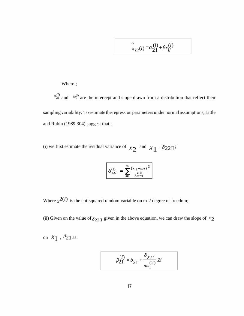
α21( )l
xl xil
li l
~ ( ) ( )( ) = +α β212
Where ;
and are the intercept and slope drawn from a distribution that reflect theirβxill( )
sampling variability. To estimate the regression parameters under normal assumptions, Little
and Rubin (1989:304) suggest that ;
(i) we first estimate the residual variance of and , ;χ2 χ1 δ22 1⋅
δχ22 1
2
1
2 2
22.
( ) ( )( )
l x x
i
mi i
ml==== −−−−
==== −−−−∑∑∑∑
Where is the chi-squared random variable on m-2 degree of freedom;χ2( )l
(ii) Given on the value of given in the above equation, we can draw the slope of δ22 1⋅χ2
on , as:χ1 β21
βδ
21 2122 1
12
( ) .( )
l bms
Zi= +

18
where Zi is a standard normal deviate ;
(iii) Given the drawn values of and , we can draw the intercept, asδ22 1⋅ β21 α21
α β δ21 21 11
22 1( ) ( )
.( )l l
ml
liy x Z==== −−−− ++++
where is an independent normal deviate.Ζ li
The reasoning behind this is that m values of replications of imputed values are used
to create m complete data matrices each of which is to be analysed by standard complete data
methods. This approach as already mentioned, retains the advantage of single imputation
by retaining a complete data set and thus allowing standards statistical methods to be used.
At the same, however, by allowing more than one value on a missing variable to be
estimated, multiple imputation corrects for sampling variability and thus improves upon
single imputation techniques which uses only a single value (Rubin and Schenker, 1986).
The imputed m values on the variable of interest can therefore be aggregated on the basis of
which a more valid statistical inference can be made. This is partly because the assumptions
under which multiple imputation operates better reflect the uncertainty due to non response.
A major advantage of this approach also relates to the fact that imputations from two or more
models for non response can be contrasted to test the sensitivity of inference especially in
situations where non-response is ‘non ignorable’. This is particularly important in instances
where one cannot empirically determine whether missing observation is ignorable or non
ignorable. Under this scenario, multiple imputation serves as a useful tool in sensitivity
analysis through which the researcher can build models under both assumptions (ignorable

19
and non ignorable) and examine which best describes the data set.
Once the predictive model has been applied m times to the data set, the question
arises as to how one might aggregate the estimates to generate the overall parameter of
interest. As Kalton and Kasprzyk (1986) have noted, this has the advantage of increasing
precision because of the aggregation over the replicates. Little and Rubin (1987, 1989) have
demonstrated that if our predictive model has been applied M times to the data with each
replicate generating , then one can estimate the overall parameter as;θi θ
θθ
mi
Mi
m=
=∑
1
where;
is the overall parameter we are imputing,θm
is the sum of the estimates produced by each replicate, and θi∑
M the number of times the model was applied.
To estimate the variance, Little and Rubin point out that variability under multiple
imputation has two components; the average within imputation variance, and between
imputation component. The average within imputation component is given as ;Wm

20
WmWtm
=∑
and between imputation variance, , is given as ;Βm
Βmi
m=
−∑−
( )θ θ 2
1
where the terms in the equation are defined as before. The total variance, , associatedSm2
with the overall parameter is estimated as;θ
S Wm m mm m2 1= + + Β
where and are defined as before, and is the finite correction factor. OnceWm Βm mm+1
the overall variance has been estimated, we can build a confidence interval around the overall
parameter, , as;θm
θ αm tv Sm± ,2
2

21
where t is a t-distribution at v degree of freedom estimated as
v m mWm
m= − + +( )[ ]1 1 1
12
Β
is based on Satterwaite approximation (Rubin, 1986, 1987; Little and Rubin, 1987; 1989).
Little and Rubin further argue that, the within and between variance ratio ( )rWmBm
=
estimates the population quality where is the fraction of information about the( )1−γ
γ γ θ
missing due to non response. Thus in an ignorable non response with no covariates,γrepresents the fraction of data values missing. Some advantages of multiple imputation arethe following; random error in the imputation process
yields approximately unbiased estimates of all parameters which no deterministic method cando.
Also, repeated imputation allows for good estimates of the standard errors.
In using the model, the question arises as to how much replications (m) ought to be
applied in order not to compromise inferences. Comparing simulation models based on
single and multiple imputation techniques, Little and Rubin (1987) and Rubin and Schenker
(1986) have demonstrated that even in extreme cases where the proportion of missing
information constitute about a third of the data set, three replicates (m=3) of the model
provides efficient estimates. Little and Rubin have noted that explicit models of multiple
imputation which we have been examining in the preceding pages might be difficult to apply
especially on large data set such as census data. Under such conditions, the researcher is
advised to use implicit multiple imputation models. For example, they suggested a variant
of the ‘hot-deck’ technique where instead of the traditional approach which substitutes a

22
closely matched respondent for a non respondent, the researcher could provide two or more
matched respondents for each incomplete case and thus allowing imputed value to be
assessed.
3.4.1 A critique of multiple imputation
Considering the advantages multiple imputation offers, it is not surprising the
technique has seen some elaborate applications (see for example, Clogg et al. 1991).
However, while acknowledging the usefulness of the technique, some researchers have been
quick in highlighting the inherent limitations (Rao, 1996a; Rao and Shao, 1992; Fay, 1991,
1996a). What Rao (1996a) regards as a limitation of multiple imputation relates to the high
cost of storage and processing and the unavailability of the Approximate Bayesian Bootstrap
(ABB) procedure for generating proper imputation. In the light of this, an alternative
‘simpler’ procedure based on jackknife variance estimation has been proposed by Rao and
Shao (1992). The jackknife variance formula, which is a modification of the ‘hot deck’
single imputation, adjusts the variance produced through single imputation to provide
suitable estimates. Fay (1996a) demonstrated that Rao and Shao technique can be extended
to multiple imputed values through Fractional Weight Adjustments (FWA). In a number of
publications, Fay has strongly argued that multiple imputed data sets should be treated as one
data set with fractional weights attached rather than creating m complete data sets envisaged
under multiple imputation (MI). In a Monte Carlo study, he demonstrated the advantages of
FWA over MI. Nonetheless, Rubin (1996a, 1996b) believes these critiques are trivial and

23
that, multiple imputation is the most effective technique for handling missing observation.
Recent debates, commentaries and rejoinders on MI, FWI, and variance estimation can be
found Binder (1996), Eltinge, (1996), Rubin (1996a, 1996b), Fay (1996a, 1996b), and Rao
(1996a, 1996b). In the midst of this confusion, one finds solace in a comment by
Binder(1996:571) that, in choosing a particular imputation technique one should realise that;
“none of the approaches is always right or always wrong and it is importantto understand the conditions under which each approach is preferred”
As Maxim also argues, it does not really matter whether one uses single or multiple
imputation, what is crucial is to find covariates that might be useful in predicting the missing
observation.
To conclude our discussion on imputation, we should mention that it is not
uncommon for the social scientist to be faced with the situation where the need arises to
impute more than one missing observation on a case. Under such scenario, the question
arises as to whether one should impute missing values independently of other missing values
or whether the value of one missing value should be made conditional on others. Many
suggested techniques for dealing with the problem involve covariance matrix through
iterative maximum likelihood approach (Maxim, 1998; Little and Rubin , 1987; Little and
Rubin, 1989). This is, however, outside the scope of this paper and those interested are
advised to consult the relevant literature.

24
4.0 Conclusions
While these approaches are, undoubtedly, ingenious ways of handling missing
observation, the best solution calls for a good research design which ultimately has the
potential to curtail, if not avoid, non response in the first place. While it is generally
acknowledged that certain forms of missing observations are obviously beyond the control
of the researcher, many instances exist where the researcher could effectively minimise the
incidence of non response in surveys. Sloppy research designs which give less thought to
methodological issues are more likely to result in a higher non response rate than a well-
designed and executed study. It is in the light of this that this researcher shares with the view
that a good research design which, for instance, focuses on pilot tests or a small sample pre-
tests through which ambiguous concepts and questions are clarified etc., are more likely to
have a higher response rates than otherwise. Also, while this writer agrees with Fay (1986)
that no single model can correctly reflect the implications of non response in all instances,
it is also worth noting that some modes of data collection are known to result in low response
rates: Platek and Gray (1985), for example, assert that telephone interviewing are more prone
to non response than personal interviews on similar subjects. The onus therefore lies on the
researcher to determine the appropriate mode of survey design taking into consideration the
subject under investigation, the target population and other relevant issues. Also, the
researcher could broaden the range of closed ended questions to make it exhaustive with the
view of capturing a sizeable number of respondents who would otherwise refuse to answer.
Again, the responsibility lies on the researcher to find more effective ways of asking
questions on sensitive issues and those that are regarded are socially undesirable. The

25
methodology literature is replete with suggested techniques for soliciting information on
undesirable issues. Further, it is suggested that if one is to rely on interviewers for data
collection, it is essential that they are properly trained in techniques of interviewing and
recording. As Maxim (1998) points out, one can have the best of designs but this can be
thrown into disarray by poorly trained interviewers who execute the project in the field.
Researchers are also advised to plan for missing data at the design stage of the study.
Familiarity with the literature on the intended study might give clues as to which variables
are prone to missing observation. Platek (1977) has, for instance, observed that finance-
related surveys tend to have lower response rates than surveys dealing with other subjects.
With such awareness, it is the opinion of this writer that the researcher can include co-
variates on the questionnaires that might be significant in predicting the missing items on
the variable in question.
To conclude, while it is true even good research designs are unlikely to result in a
100 percent response rates, undoubtedly, non response under the control of the researcher
will be seriously minimised. Nonetheless, if the need arises to impute missing observations
using any of the suggested techniques in this paper, the researcher should be mindful of the
assumptions underlying the particular technique and the type of variable being imputed.
Always, one should be mindful of the fact that irrespective of the technique one uses,
imputed values should always be interpreted with caution and should not be regarded as real.

26
BIBLIOGRAPHY
Binder, D.A. (1996). Comment. Journal of the American Statistical Association, Vol. 91,No. 434:510-512.
Buck, S.F. (1960). A method of estimating missing values in multivariate data suitable foruse with an electronic computer. Journal of Royal Statistical Society, B22:302-306
Brown, R.L. (1994). Efficacy of indirect approach for estimating structural equation modelwith missing data: A comparison of five methods. Structural Equation Modelling:A Multidisciplinary Journal, 1:287-316.
Chiu, H.Y., and J Sedransk (1986). A Bayesian procedure for imputing missing values insample values in sample surveys. Journal of the American Statistical Association,Vol. 81, No. 395:667- 676.
Clogg, C.C., D.B. Rubin, N. Schenker, B. Schultz, and L. Neidman (1991). Multipleimputation of industry and occupation codes in census public-use samples usingBayesian logistic regression. Journal of the American Statistical Association, Vol.86, No. 413:68- 78.
Dempster, A.P. and Rubin, D.B.(1983). Overview of Incomplete Data in Sample Surveys,Vol.II Theory and Annotated Bibliography. W.G. Madow, I. Olkin, and D.BRubin (Eds.), New York:Academic Press, 3-10.
Dodge, Y. (1985) Analysis of Experiments with Missing Data. New York: Willey Series inProbability and Mathematical Statistics
Eltinge, J. (1996). Comment. Journal of the American Statistical Association, Vol. 91,No.434:513-514.
Fay, R.E. (1986). Causal models for patterns of non response. Journal of the StatisticalAssociation of America, Vol. 81, No.394:355-365
Fay, R.E. (1996a). Alternative paradigms for the analysis of imputed survey data. Journalof the American Statistical Association, Vol. 91, No.434:490-498.
Fay, R.E. (1996b). Rejoinder. Journal of the American Statistical Association, Vol. 91,No.434:517-519.
Ford, B. (1983). “An Overview of Hot-deck Procedures” in Incomplete Data in SampleSurvey, vol II eds W.G. Madow, I. Olkin, and D.B Rubin

27
Glasser, M. (1964). Linear regression analysis with missing observations among theindependent variables. Journal of the American Statistical Association, Vol.59:834-844.
Grischilles, Z. (1986). “Economic data issues” In Grischilles, Z. and M. Intilligator (Eds.),Handbook of Econometrics. Vol. 3. Amsterdam
Greenless, John, S., William S. Pierce and Kimberly d. Zieschang (1982). Imputation ofmissing values when the probability of response depends on the variable beingimputed. Journal of the American Statistical Association, Vol.77, No.378:251-261.
Haitovsky, Y. (1968) Missing data in regression analysis. Royal Statistical Society. LondonB, 30:67-82
Horst, Paul (1968). The Missing data matrix. Journal of Clinical Psychology, MonographSupplement, Number 26, July 1986:286-306.
Kalton, G. and David Kasprszyk (1982). Imputing for Missing Data in Proceedings of theSection on Survey Methods, American Statistical Association, 22-31.
Kalton, G. and David Kasprszyk (1986). The treatment of missing survey data. SurveyMethodology, vol.12, No.1:1-16
Little, Roderick, A. (1985). Modelling drop-out mechanism in repeated measures studies.Journal of the American Statistical Studies, Vol. 90, No.431:1112-1121.
Little, Roderick,J.A. and Donald B, Rubin (1987). Statistical Analysis with Missing Data.New York. John Willey and Sons.
Little, Roderick,J.A. and Donald B, Rubin (1989). Analysis of social science data withmissing values. Sociological Methods and Research, 18:292-326.
Madow, William G., Harold Nisselson and Ingram Olkin (Eds., 1983). Incomplete Data inSample Surveys. Vol.1 Report and Case Studies.
Maxim, Paul (1998). Lecture Notes on Quantitative and Empirical Sociology, University ofWestern Ontario, London, On.
Platek, R. (1977). Some Factors Affecting Non-response. Paper presented at theInternational Statistical Institute, New Delhi, December.
Platek, R. and G.B. Gray (1986). On the definition of response rate. Survey Methodology,Vol.12, No.1:17-27.

28
Orchard, T. and Woodbury, M.A. (1972). A Missing Information Principle: Theory andApplications. Proceedings of the sixth Berkeley Symposium on MathematicalStatistics and Probability, Theory of Statistics, University of California Press.
Kim, Jae-On and James Curry (1977). The treatment of missing data in multivariateanalysis. Sociological Methods and Research, 6:206-240
Rao, J.N.K. (1996a). On variance estimation with imputed survey data. Journal of theAmerican Statistical Association, Vol.91, No.434:499-506.
Rao, J.N.K. (1996b). Rejoinder. Journal of the American Statistical Association, Vol.91,No.434:519-520.
Rao, J.N.K. and J. Shao (1992). Jackknife variance estimation with survey data under hot-deck imputation. Biometrika, 79:811-822
Rubin, D.B. (1977). Formalizing subjective notions about the effect on non respondents insample surveys. Journal of the American Statistical Association, 72:538-543
Rubin, Donald, B.(1986).Basic ideas of multiple imputation on non-response. SurveyMethodology, Vol. 12, No.1:37- 47
Rubin, D.B (1987). Multiple Imputation for Nonresponse in Surveys. New York: JohnWilley and Sons.
Rubin, Donald(1996a). Multiple imputation 18+ years. Journal of the American StatisticalAssociation, Vol.91, No.434:473-489.
Rubin, Donald (1996b). Rejoinder, Journal of the American Statistical Association, Vol.91,No.434:515-517.
Rubin, D.B. and N. Schenker (1986). Multiple imputation from random samples withignorable non response. Journal of the American Statistical Association, Volume 81,No.394:366-374.
Vach, W. (1994). Logistic Regression with Missing Values in the Covariates. New York:Sprnger-Verlag.