mme313 chapter6 sm
TRANSCRIPT
Chapter 6 • Viscous Flow in Ducts
P6.1 An engineer claims that flow of SAE 30W oil, at 20°C, through a 5-cm-diameter smooth pipe at 1 million N/h, is laminar. Do you agree? A million newtons is a lot, so this sounds like an awfully high flow rate.
Solution: For SAE 30W oil at 20°C (Table A.3), take ρ = 891 kg/m3 and μ = 0.29 kg/m-s. Convert the weight flow rate to volume flow rate in SI units:
)(/29.0
)05.0)(/2.16)(/891(Re
2.16,)05.0(4
0318.0)/81.9)(/891()/3600/1)(/61(
3
23
23
altransitionsmkg
msmmkgVDCalculate
smVsolveVm
sm
smmkgshhNE
gwQ
D 2500≈−
==
=====
μρ
πρ
This is not high, but not laminar. Ans. With careful inlet design, low disturbances, and a very smooth wall, it might still be laminar, but No, this is transitional, not definitely laminar.
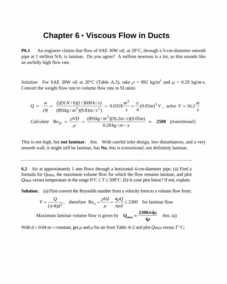
6.2 Air at approximately 1 atm flows through a horizontal 4-cm-diameter pipe. (a) Find a formula for Qmax, the maximum volume flow for which the flow remains laminar, and plot Qmax versus temperature in the range 0°C ≤ T ≤ 500°C. (b) Is your plot linear? If not, explain.
Solution: (a) First convert the Reynolds number from a velocity form to a volume flow form:
24, therefore Re 2300 for laminar flow
( /4) dQ Vd QV
ddρ ρ
μ πμπ= = = ≤
Maximum laminar volume flow is given by . (a)Ansmax2300Q
4=
π μρ
d
With d = 0.04 m = constant, get μ and ρ for air from Table A-2 and plot Qmax versus T °C:

Chapter 6 • Viscous Flow in Ducts 435
Fig. P6.2
The curve is not quite linear because ν = μ/ρ is not quite linear with T for air in this range. Ans. (b)
6.3 For a thin wing moving parallel to its chord line, transition to a turbulent boundary layer occurs at a “local” Reynolds number Rex, where x is the distance from the leading edge of the wing. The critical Reynolds number depends upon the intensity of turbulent fluctuations in the stream and equals 2.8E6 if the stream is very quiet. A semiempirical correlation for this case [Ref. 3 of Ch. 6] is
crit1/2
21 (1 13.25 )Re
0.00392xζ
ζ− + +
≈2 1/2
where ζ is the tunnel-turbulence intensity in percent. If V = 20 m/s in air at 20°C, use this formula to plot the transition position on the wing versus stream turbulence for ζ between 0 and 2 percent. At what value of ζ is xcrit decreased 50 percent from its value at ζ = 0?
Solution: This problem is merely to illustrate the strong effect of stream turbulence on the transition point. For air at 20°C, take ρ = 1.2 kg/m3 and μ = 1.8E−5 kg/m⋅s. Compute Rex,crit from the correlation and plot xtr = μRex/[ρ(20 m/s)] versus percent turbulence:

436 Solutions Manual • Fluid Mechanics, Fifth Edition
Fig. P6.3
The value of xcrit decreases by half (to 1.07 meters) at ζ ≈ 0.42%. Ans.
6.4 For flow of SAE 30 oil through a 5-cm-diameter pipe, from Fig. A.1, for what flow rate in m3/h would we expect transition to turbulence at (a) 20°C and (b) 100°C?
Solution: For SAE 30 oil take and take μ = 0.29 kg/m⋅s at 20°C (Table A.3) and 0.01 kg/m-s at 100°C (Fig A.1). Write the critical Reynolds number in terms of flow rate Q:
3891 kg/mρ =
34 4(891 / )(a) Re 2300 ,VD Q kg m Qm
s
ρ ρ= = = =
3 3(0.29 / )(0.05 )
solve 0.0293 . (a)
crit D kg m smQ Ans
μ πμ π ⋅
= =m106h
34 4(891 / )(b) Re 2300 ,critVD Q kg m Q
m
s
ρ ρ= = = =
3
(0.010 / )(0.05 )
solve 0.00101 . (b)
D kg m s
mQ Ans
μ πμ π ⋅
= =3m3.6
h
Chapter 6 • Viscous Flow in Ducts 437
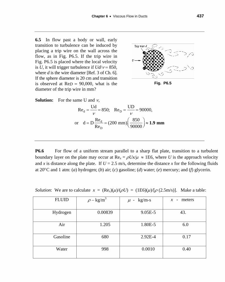
6.5 In flow past a body or wall, early transition to turbulence can be induced by placing a trip wire on the wall across the flow, as in Fig. P6.5. If the trip wire in Fig. P6.5 is placed where the local velocity is U, it will trigger turbulence if Ud/ν = 850, where d is the wire diameter [Ref. 3 of Ch. 6]. If the sphere diameter is 20 cm and transition is observed at ReD = 90,000, what is the diameter of the trip wire in mm?
Fig. P6.5
Solution: For the same U and ν,
d DUd UDRe 850; Re 90000,= = = =
d
D
Re 850or d D (200 mm) Re 90000
ν ν⎛ ⎞= = ≈⎜ ⎟⎝ ⎠
1.9 mm
P6.6 For flow of a uniform stream parallel to a sharp flat plate, transition to a turbulent boundary layer on the plate may occur at Rex = ρUx/μ ≈ 1E6, where U is the approach velocity and x is distance along the plate. If U = 2.5 m/s, determine the distance x for the following fluids at 20°C and 1 atm: (a) hydrogen; (b) air; (c) gasoline; (d) water; (e) mercury; and (f) glycerin.
Solution: We are to calculate x = (Rex)(μ)/(ρU) = (1E6)(μ)/[ρ (2.5m/s)]. Make a table:
FLUID ρ – kg/m3 μ - kg/m-s x - meters
Hydrogen 0.00839 9.05E-5 43.
Air 1.205 1.80E-5 6.0
Gasoline 680 2.92E-4 0.17
Water 998 0.0010 0.40
438 Solutions Manual • Fluid Mechanics, Fifth Edition
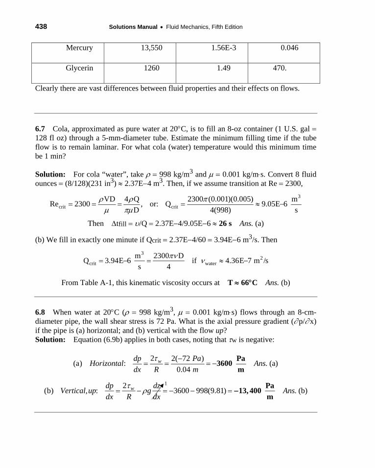
Mercury 13,550 1.56E-3 0.046
Glycerin 1260 1.49 470.
Clearly there are vast differences between fluid properties and their effects on flows.
6.7 Cola, approximated as pure water at 20°C, is to fill an 8-oz container (1 U.S. gal = 128 fl oz) through a 5-mm-diameter tube. Estimate the minimum filling time if the tube flow is to remain laminar. For what cola (water) temperature would this minimum time be 1 min?
Solution: For cola “water”, take ρ = 998 kg/m3 and μ = 0.001 kg/m⋅s. Convert 8 fluid ounces = (8/128)(231 in3) ≈ 2.37E−4 m3. Then, if we assume transition at Re = 2300,
3
crit critVD 4 Q 2300 (0.001)(0.005) mRe 2300 , or: Q 9.05E 6
D 4(998) sρ ρ π
μ πμ= = = = ≈ −
Then Δtfill = υ/Q = 2.37E−4/9.05E−6 ≈ 26 s Ans. (a)
(b) We fill in exactly one minute if Qcrit = 2.37E−4/60 = 3.94E−6 m3/s. Then 3
2crit water
m 2300 DQ 3.94E 6 if 4.36E 7 m /ss 4
πν ν= − = ≈ −
From Table A-1, this kinematic viscosity occurs at T ≈ 66°C Ans. (b)
6.8 When water at 20°C (ρ = 998 kg/m3, μ = 0.001 kg/m⋅s) flows through an 8-cm-diameter pipe, the wall shear stress is 72 Pa. What is the axial pressure gradient (∂ p/∂ x) if the pipe is (a) horizontal; and (b) vertical with the flow up? Solution: Equation (6.9b) applies in both cases, noting that τw is negative:
2 2( 72 )(a) : (a)0.04
wdp PaHorizontal Ans.dx R m
τ −= = = −
Pa3600m
2(b) : 3600= − 998(9.81) (b)wdp dzVertical, up g Ans.dx R dx
τρ= − − =
Pa13, 400m
−
1

Chapter 6 • Viscous Flow in Ducts 439
6.9 A light liquid (ρ = 950 kg/m3) flows at an average velocity of 10 m/s through a horizontal smooth tube of diameter 5 cm. The fluid pressure is measured at 1-m intervals along the pipe, as follows:
x, m: 0 1 2 3 4 5 6 p, kPa: 304 273 255 240 226 213 200
Estimate (a) the total head loss, in meters; (b) the wall shear stress in the fully developed section of the pipe; and (c) the overall friction factor.
Solution: As sketched in Fig. 6.6 of the text, the pressure drops fast in the entrance region (31 kPa in the first meter) and levels off to a linear decrease in the “fully developed” region (13 kPa/m for this data). (a) The overall head loss, for Δz = 0, is defined by Eq. (6.8) of the text:
ρΔ −
= = =3 2304,000 200,000 (a)(950 / )(9.81 / )f
p Pah Ans.g kg m m s
11.2 m
(b) The wall shear stress in the fully-developed region is defined by Eq. (6.9b):
4 413000 , solve for (b)
1 0.05 w w
fully developed wp Pa Ans.L m d m
τ ττΔ
= = = =Δ
| 163 Pa
(c) The overall friction factor is defined by Eq. (6.10) of the text:
2
, 2 22 0.05 2(9.81 / )(11.2 ) (c)
6 (10 / )overall f overalld g m m sf h m Ans.L mV m s
⎛ ⎞= = =⎜ ⎟⎝ ⎠
0.0182
NOTE: The fully-developed friction factor is only 0.0137.
6.10 Water at 20°C (ρ = 998 kg/m3) flows through an inclined 8-cm-diameter pipe. At sections A and B, pA = 186 kPa, VA = 3.2 m/s, zA = 24.5 m, while pB = 260 kPa, VB BB = 3.2 m/s, and zB = 9.1 m. Which way is the flow going? What is the head loss?
Solution: Guess that the flow is from A to B and write the steady flow energy equation:
2 2 186000 260000, or: 24.5 9.1 ,
: , . . (a, b)
A A B BA B f f
p V p Vz z h hg g g g
or Yes flow is from A to B Ans
ρ ρ+ + = + + + + = + +
fh 7.84 m= +
2 2 9790 9790
: 43.50
35.66 , solvefh= +
440 Solutions Manual • Fluid Mechanics, Fifth Edition
6.11 Water at 20°C flows upward at 4 m/s in a 6-cm-diameter pipe. The pipe length between points 1 and 2 is 5 m, and point 2 is 3 m higher. A mercury manometer, connected between 1 and 2, has a reading h = 135 mm, with p1 higher. (a) What is the pressure change (p1 − p2)? (b) What is the head loss, in meters? (c) Is the manometer reading proportional to head loss? Explain. (d) What is the friction factor of the flow?
Solution: A sketch of this situation is shown at right. By moving through the manometer, we obtain the pressure change between points 1 and 2, which we compare with Eq. (6.9b):
1 2,w m wp h h z pγ γ γ+ − − Δ =
1 2 3 3 133100 9790 (0.135 ) 9790 (3 )
16650 29370 (a)
p p m mm m
Ans.
− = − +⎜ ⎟ ⎜⎝ ⎠ ⎝
= + =
or:
46,000 Pa
N N⎛ ⎞ ⎛ ⎞⎟⎠
346000 . , 3 4.7 3.0 (b)
9790 /fw
p PaFrom Eq (6.9b) h z m Ans.N mγ
Δ= − Δ = − = − = 1.7 m
2
2 22 0.06 2(9.81 / )(1.7 ) (d)
5 (4 / )fd g m m sThe friction factor is f h m Ans.L mV m s
⎛ ⎞= = =⎜ ⎟⎝ ⎠0.025
By comparing the manometer relation to the head-loss relation above, we find that:
( ) (c)m wf
wh h Aγ γ
γ−
= isand thus head loss proportional to manometer reading. ns.
NOTE: IN PROBLEMS 6.12 TO 6.99, MINOR LOSSES ARE NEGLECTED.
6.12 A 5-mm-diameter capillary tube is used as a viscometer for oils. When the flow rate is 0.071 m3/h, the measured pressure drop per unit length is 375 kPa/m. Estimate the viscosity of the fluid. Is the flow laminar? Can you also estimate the density of the fluid?
Solution: Assume laminar flow and use the pressure drop formula (6.12):
4 4? ?p 8Q Pa 8(0.071/3600), or: 375000 , solve .
L mR (0.0025)Ansμ μ μ
π πΔ
= = ≈kg0.292m s⋅

Chapter 6 • Viscous Flow in Ducts 441
oilkgGuessing 900 ,3m
4 Q 4(900)(0.071/3600)check Re .d (0.292)(0.005)
Ansρπμ π
= = ≈ 16 OK, laminar
ρ ≈
It is not possible to find density from this data, laminar pipe flow is independent of density.
6.13 A soda straw is 20 cm long and 2 mm in diameter. It delivers cold cola, approximated as water at 10°C, at a rate of 3 cm3/s. (a) What is the head loss through the straw? What is the axial pressure gradient ∂p/∂x if the flow is (b) vertically up or (c) horizontal? Can the human lung deliver this much flow?
Solution: For water at 10°C, take ρ = 1000 kg/m3 and μ = 1.307E−3 kg/m⋅s. Check Re: 34 Q 4(1000)(3E 6 m /s)Re 1460 (OK, laminar flow)
d (1.307E 3)(0.002)ρ
πμ π−
= = =−
f 4 4128 LQ 128(1.307E 3)(0.2)(3E 6)Then, from Eq. (6.12), h (a)
gd (1000)(9.81)(0.002)Ans.μ
πρ π− −
= = ≈ 0.204 m
If the straw is horizontal, then the pressure gradient is simply due to the head loss:
fhoriz
p gh 1000(9.81)(0.204 m) (c)L L 0.2 m
Ans.ρΔ= = ≈| Pa9980
m
If the straw is vertical, with flow up, the head loss and elevation change add together:
fvertical
p g(h z) 1000(9.81)(0.204 0.2) (b)L L 0.2
Ans.ρΔ + Δ += = ≈| Pa19800
m
The human lung can certainly deliver case (c) and strong lungs can develop case (b) also.

442 Solutions Manual • Fluid Mechanics, Fifth Edition
6.14 Water at 20°C is to be siphoned through a tube 1 m long and 2 mm in diameter, as in Fig. P6.14. Is there any height H for which the flow might not be laminar? What is the flow rate if H = 50 cm? Neglect the tube curvature.
Fig. P6.14
Solution: For water at 20°C, take ρ = 998 kg/m3 and μ = 0.001 kg/m⋅s. Write the steady flow energy equation between points 1 and 2 above:
22 2 32 L Vatm atm tube
1 2 f f 2p p V0 Vz z h , or: H h
g 2g g 2g 2g gdμ
ρ ρ ρ+ + = + + + − = = (1)
2
2V 32(0.001)(1.0)V mEnter data in Eq. (1): 0.5 , solve V 0.590
2(9.81) s(998)(9.81)(0.002)− = ≈
Equation (1) is quadratic in V and has only one positive root. The siphon flow rate is 3
2H=50 cm
mQ (0.002) (0.590) 1.85E 6 .4 s
Ansπ= = − ≈
m0.0067 if 50 cmh
H =3
Check Re (998)(0.590)(0.002) /(0.001) 1180 (OK, laminar flow)= ≈
It is possible to approach Re ≈ 2000 (possible transition to turbulent flow) for H < 1 m, for the case of the siphon bent over nearly vertical. We obtain Re = 2000 at H ≈ 0.87 m.
6.15 Professor Gordon Holloway and his students at the University of New Brunswick went to a fast-food emporium and tried to drink chocolate shakes (ρ ≈ 1200 kg/m3, μ ≈ 6 kg/m⋅s) through fat straws 8 mm in diameter and 30 cm long. (a) Verify that their human lungs, which can develop approximately 3000 Pa of vacuum pressure, would be unable to drink the milkshake through the vertical straw. (b) A student cut 15 cm from his straw and proceeded to drink happily. What rate of milkshake flow was produced by this strategy?
Solution: (a) Assume the straw is barely inserted into the milkshake. Then the energy equation predicts
2 21 1 2 2
1 2 f
2
3 2
2 2
( 3000 )0 0 0 0.3 2(1200 / )(9.81 / )tube
f
p V p Vz z h= + = = + +g g g g
VPa m hgkg m m s
ρ ρ
−= + + = + + +
(a)Solve for Ans.tubef
V h m m which is impossibleg
= − − <0.255 0.3 02
2

Chapter 6 • Viscous Flow in Ducts 443
(b) By cutting off 15 cm of vertical length and assuming laminar flow, we obtain a new energy equation
2 2V2 2
32 32(6.0)(0.15)0.255 0.15 0.105 38.232 2(9.81) (1200)(9.81)(0.008)fV LV V Vh m
g gdμ
ρ= − − = = − = =
2Solve for 0.00275 / , ( /4)(0.008) (0.00275)
V m s Q AV π= = =3
1.4 7 (b)mQ E Ans.s
= − =3cm0.14
s
Check the Reynolds number: Red = ρVd/μ = (1200)(0.00275)(0.008)/(6) = 0.0044 (Laminar).
6.16 Glycerin at 20°C is to be pumped through a horizontal smooth pipe at 3.1 m3/s. It is desired that (1) the flow be laminar and (2) the pressure drop be no more than 100 Pa/m. What is the minimum pipe diameter allowable?
Solution: For glycerin at 20°C, take ρ = 1260 kg/m3 and μ = 1.49 kg/m⋅s. We have two different constraints to satisfy, a pressure drop and a Reynolds number:
4 4p 128 Q Pa 128(1.49)(3.1)100 (1); 100, ,
L md dμ
π πΔ
= ≤ ≤ d 1.17 m≥
;4 Q 4(1260)(3.1)or: Re 2000 (2) 2000,
d (1.49)dρ
πμ π= ≤ ≤ d 1.67 m≥
The second of these is more restrictive. Thus the proper diameter is d ≥ 1.67 m. Ans.
6.17 A capillary viscometer measures the time required for a specified volume υ of liquid to flow through a small-bore glass tube, as in Fig. P6.17. This transit time is then correlated with fluid viscosity. For the system shown, (a) derive an approximate formula for the time required, assuming laminar flow with no entrance and exit losses. (b) If L = 12 cm, l = 2 cm, υ = 8 cm3, and the fluid is water at 20°C, what capillary diameter D will result in a transit time t of 6 seconds?
Fig. P6.17
444 Solutions Manual • Fluid Mechanics, Fifth Edition
Solution: (a) Assume no pressure drop and neglect velocity heads. The energy equation reduces to:
2 2L l1 1 2 2
1 20 0 ( ) 0 0 0 , :2 2 f f f
p V p Vz L l z h h hg g g gρ ρ
+ + = + + + = + + + = + + + ≈ +or
4128, ,f
LQFor laminar flow h and, for uniform draining Qtgd
μ υπρ
= =Δ
(a)Solve for Ans.L tgd L l
Δ =+4
128( )μ υ
πρ
(b) Apply to Δt = 6 s. For water, take ρ = 998 kg/m3 and μ = 0.001 kg/m⋅s. Formula (a) predicts: 3128(0.001 / )(0.12 )(8 6 )kg m s m E m⋅ −
3 2 46 ,(998 / )(9.81 / ) (0.12 0.02 )
Solve for (b)
t skg m m s d m
Ans.
πΔ = =
+
d 0.0015 m≈
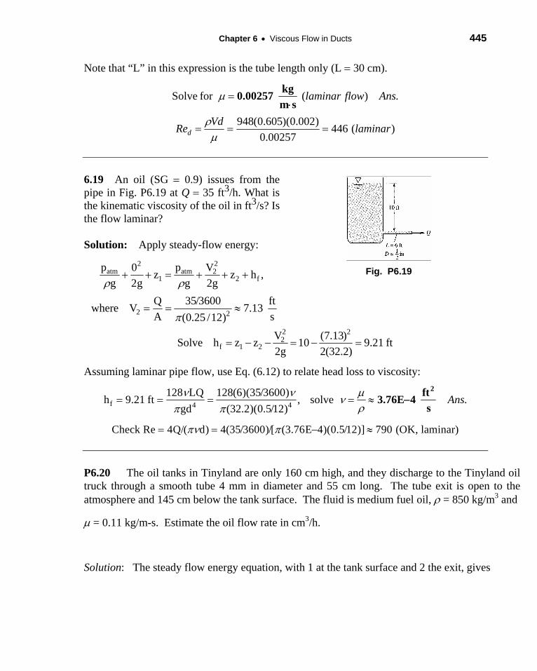
6.18 To determine the viscosity of a liquid of specific gravity 0.95, you fill, to a depth of 12 cm, a large container which drains through a 30-cm-long vertical tube attached to the bottom. The tube diameter is 2 mm, and the rate of draining is found to be 1.9 cm3/s. What is your estimate of the fluid viscosity? Is the tube flow laminar?
Fig. P6.18
Solution: The known flow rate and diameter enable us to find the velocity in the tube:
3 m2
1.9 6 / 0.605 ( /4)(0.002 )
Q E m sVA smπ
−= = =
Evaluate ρ liquid = 0.95(998) = 948 kg/m3. Write the energy equation between the top surface and the tube exit:
2 2
2 2
0 ,2 2
32 (0.3)(0.605): 0.42.81) 948(9.81)(0.002)
topa atop f
Vp p Vz hg g g g
org
ρ ρ
μ μ
= + = + + +
= + +2 232 (0.605)
2 2(9V LV
gdρ=
Chapter 6 • Viscous Flow in Ducts 445
Note that “L” in this expression is the tube length only (L = 30 cm).
Solve for ( )laminar flow Ans.
948(0.605)(0.002) 446 ( )0.00257d
VdRe laminarρμ
= = =
m s⋅μ =
kg0.00257
6.19 An oil (SG = 0.9) issues from the pipe in Fig. P6.19 at Q = 35 ft3/h. What is the kinematic viscosity of the oil in ft3/s? Is the flow laminar?
Solution: Apply steady-flow energy:
2 2
fh ,atm atm 21 2
p p0 Vz zg 2g g 2gρ ρ
+ + = + + + Fig. P6.19
2 2Q 35/3600 ftwhere V 7.13 A s(0.25 /12)π
= = ≈
2 22
f 1 2V (7.13)Solve h z z 10 9.21 ft2g 2(32.2)
= − − = − =
Assuming laminar pipe flow, use Eq. (6.12) to relate head loss to viscosity:
f 4 4128 LQ 128(6)(35/3600)h 9.21 ft , solve
gd (32.2)(0.5/12)Ans.ν ν μν
ρπ π= = = = ≈
ft3.76E 4s
−2
Check Re 4Q/( d) 4(35/3600)/[ (3.76E 4)(0.5/12)] 790 (OK, laminar)πν π= = − ≈
P6.20 The oil tanks in Tinyland are only 160 cm high, and they discharge to the Tinyland oil truck through a smooth tube 4 mm in diameter and 55 cm long. The tube exit is open to the atmosphere and 145 cm below the tank surface. The fluid is medium fuel oil, ρ = 850 kg/m3 and
μ = 0.11 kg/m-s. Estimate the oil flow rate in cm3/h.
Solution: The steady flow energy equation, with 1 at the tank surface and 2 the exit, gives
446 Solutions Manual • Fluid Mechanics, Fifth Edition
11.0)004.0(850Re,)
004.055.0
Re640.2(
245.1:,
22
222
21V
mm
gVmzor
gV
dLf
gVzz d
d=+==Δ++=
α
We have taken the energy correction factor α = 2.0 for laminar pipe flow.
Solve for V = 0.10 m/s, Red = 3.1 (laminar), Q = 1.26E-6 m3/s ≈ 4500 cm3/h. Ans.
The exit jet energy αV2/2g is properly included but is very small (0.001 m).
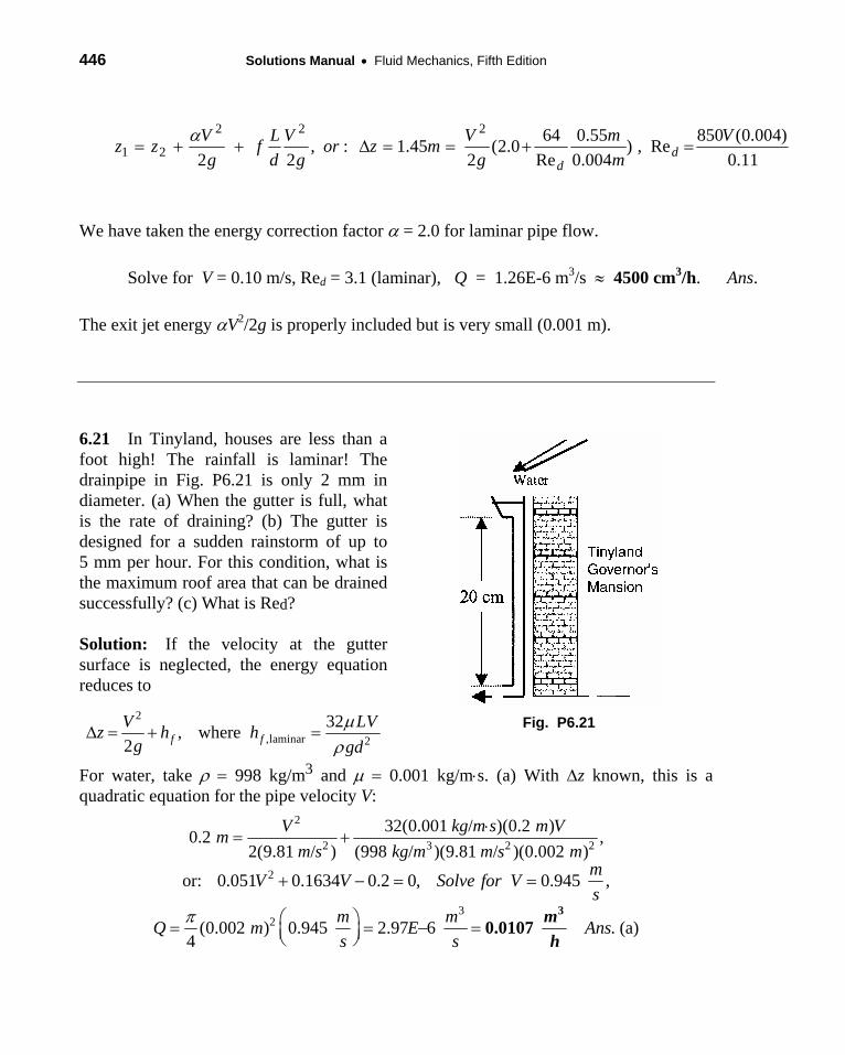
6.21 In Tinyland, houses are less than a foot high! The rainfall is laminar! The drainpipe in Fig. P6.21 is only 2 mm in diameter. (a) When the gutter is full, what is the rate of draining? (b) The gutter is designed for a sudden rainstorm of up to 5 mm per hour. For this condition, what is the maximum roof area that can be drained successfully? (c) What is Red?
Solution: If the velocity at the gutter surface is neglected, the energy equation reduces to
2
,laminar 232, where
2 f fV LVz h h
g gdμ
ρΔ = + =
Fig. P6.21
For water, take ρ = 998 kg/m3 and μ = 0.001 kg/m⋅s. (a) With Δz known, this is a quadratic equation for the pipe velocity V:
2
2m V
2 3 232(0.001 / )(0.2 )0.2 ,
2(9.81 / ) (998 / )(9.81 / )(0.002 )V kg m sm
m s kg m m s m⋅
= +
or 2: 0.051 0.1634 0.2 0, 0.945 ,mV V Solve for V
s+ − = =
3s.
32(0.002 ) 0.945 2.97 6 (a)
4m mQ m E Ans s
π ⎛ ⎞= = − =⎜ ⎟⎝ ⎠0.0107 m
h

Chapter 6 • Viscous Flow in Ducts 447
(b) The roof area needed for maximum rainfall is 0.0107 m3/h ÷ 0.005 m/h = 2.14 m2. Ans. (b) (c) The Reynolds number of the gutter is Red = (998)(0.945)(0.002)/(0.001) = 1890 laminar. Ans. (c)
6.22 A steady push on the piston in Fig. P6.22 causes a flow rate Q = 0.15 cm3/s through the needle. The fluid has ρ = 900 kg/m3 and μ = 0.002 kg/(m⋅s). What force F is required to maintain the flow?
Fig. P6.22
Solution: Determine the velocity of exit from the needle and then apply the steady-flow energy equation:
1 2Q 0.15 306 cm/sA ( /4)(0.025)
Vπ
= = =
2 2
f22 2 1 1
2 1 f1 f2 1 2 2p V p VEnergy: z z h h , with z z , V 0, h 0
g 2g g 2gρ ρ+ + = + + + + = ≈ ≈
Assume laminar flow for the head loss and compute the pressure difference on the piston: 2 2
2 1 1f1 2
p p V 32(0.002)(0.015)(3.06) (3.06)h 5.79 mg 2g 2(9.81)(900)(9.81)(0.00025)ρ
−= + = + ≈
2pistonThen F pA (900)(9.81)(5.79) (0.01)
4Ans.π
= Δ = ≈ 4.0 N
6.23 SAE 10 oil at 20°C flows in a vertical pipe of diameter 2.5 cm. It is found that the pressure is constant throughout the fluid. What is the oil flow rate in m3/h? Is the flow up or down?
Solution: For SAE 10 oil, take ρ = 870 kg/m3 and μ = 0.104 kg/m⋅s. Write the energy equation between point 1 upstream and point 2 downstream:
2 2
1 21 1 2 2
1 2 f 1 2p V p Vz z h , with p p and V Vg 2g g 2gρ ρ
+ + = + + + = =
448 Solutions Manual • Fluid Mechanics, Fifth Edition
f 1 2Thus h z z 0 by definition. Therefore, . .Ans= − > flow is down
While flowing down, the pressure drop due to friction exactly balances the pressure rise due to gravity. Assuming laminar flow and noting that Δz = L, the pipe length, we get
f 4
4 3
128 LQh z L,gd
(8.70)(9.81)(0.025) mor: Q 7.87E 4 128(0.104) s
Ans.
μπρ
π
= = Δ =
= = − =3m2.83
h
6.24 Two tanks of water at 20°C are connected by a capillary tube 4 mm in diameter and 3.5 m long. The surface of tank 1 is 30 cm higher than the surface of tank 2. (a) Estimate the flow rate in m3/h. Is the flow laminar? (b) For what tube diameter will Red be 500? Solution: For water, take ρ = 998 kg/m3 and μ = 0.001 kg/m⋅s. (a) Both tank surfaces are at atmospheric pressure and have negligible velocity. The energy equation, when neglecting minor losses, reduces to:
4 3 2128 128(0.001 / )(3.5 )0.3
(998 / )(9.81 / )(0.004 )fLQ kg m s m Qz m h
gd kg m m s mμ
πρ π⋅
Δ = = = = 4
3 3Solve for 5.3 6 (a)mQ E Ans.
s= − =
m0.019h
dCheck Re 4 /( ) 4(998)(5.3E 6)/[ (0.001)(0.004)] (a)
Q dAns.
ρ πμ π= = −
1675dRe = laminar.
(b) If Red = 500 = 4ρQ/(πμd) and Δz = hf, we can solve for both Q and d: 34(998 / )Re 500 , 0.000394
(0.001 / )dkg m Q Q dkg m s dπ
= = =⋅
or
43 2 4
128(0.001 / )(3.5 )0.3 , 20600(998 / )(9.81 / )f
kg m s m Qh m or Qkg m m s dπ
⋅= = = d
31.05 6 / (b)Combine these two to solve for Q E m s and Ans.= − d 2.67 mm=
Chapter 6 • Viscous Flow in Ducts 449
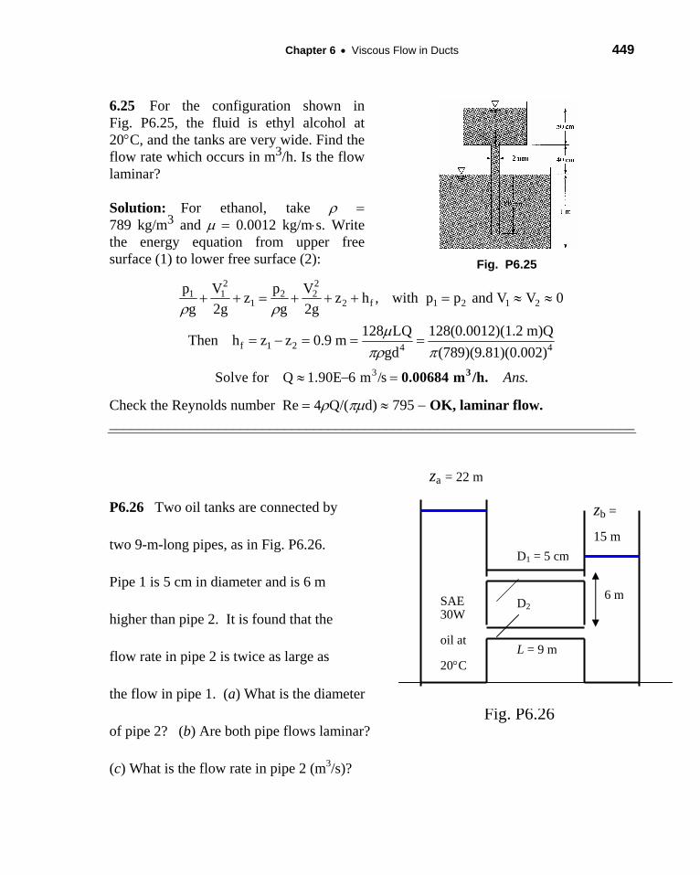
6.25 For the configuration shown in Fig. P6.25, the fluid is ethyl alcohol at 20°C, and the tanks are very wide. Find the flow rate which occurs in m3/h. Is the flow laminar?
Solution: For ethanol, take ρ = 789 kg/m3 and μ = 0.0012 kg/m⋅s. Write the energy equation from upper free surface (1) to lower free surface (2):
Fig. P6.25
2 2
21 1 2 2
1 2 f 1 2 1p V p Vz z h , with p p and V V 0g 2g g 2gρ ρ
+ + = + + + = ≈ ≈
f 1 2 4 4128 LQ 128(0.0012)(1.2 m)QThen h z z 0.9 m
gd (789)(9.81)(0.002)μ
πρ π= − = = =
3Solve for Q 1.90E 6 m /s .Ans≈ − = 30.00684 m /h.
Check the Reynolds number Re = 4ρQ/(πμd) ≈ 795 − OK, laminar flow. ________________________________________________________________________
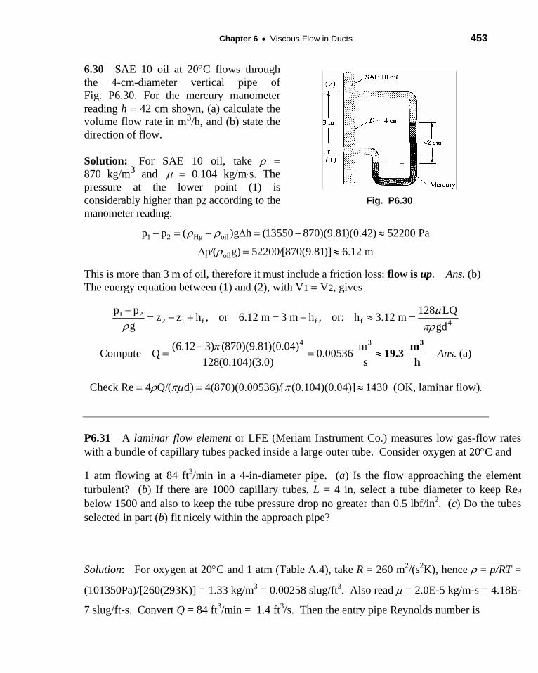
za = 22 m
P6.26 Two oil tanks are connected by zb =
15 m two 9-m-long pipes, as in Fig. P6.26. D1 = 5 cm
Pipe 1 is 5 cm in diameter and is 6 m 6 mSAE
30W
oil at
20°C
D2
higher than pipe 2. It is found that the
L = 9 m flow rate in pipe 2 is twice as large as
the flow in pipe 1. (a) What is the diameter Fig. P6.26
of pipe 2? (b) Are both pipe flows laminar?
(c) What is the flow rate in pipe 2 (m3/s)?

450 Solutions Manual • Fluid Mechanics, Fifth Edition
Neglect minor losses.
Solution: (a) If we know the flows are laminar, and (L, ρ, μ) are constant, then Q ∝ D4:
).()0.2)(5(hence,)(0.2,(6.12)Eq.From 4/12
4
1
2
1
2 aAnscmDDD
QQ cm5.95====
We will check later in part (b) to be sure the flows are laminar. [Placing pipe 1 six
meters higher was meant to be a confusing trick, since both pipes have exactly the same
head loss and Δz.] (c) Find the flow rate first and then backtrack to the Reynolds
numbers. For SAE 30W oil at 20°C (Table A.3), take ρ = 891 kg/m3 and μ = 0.29 kg/m-
s. From the energy equation, with V1 = V2 = 0, and Eq. (6.12) for the laminar head loss,
).(foSolve
)0595.0)(/81.9)(/891()9)(/29.0(12812871522
2
4232
42
cAnsQr
msmmkgQmsmkg
gDLQhmz f
/sm0.0072 3=
−====−=Δ
ππρμ
In a similar manner, insert D1 = 0.05m and compute Q1 = 0.0036 m3/s = (1/2)Q1. (b) Now go back and compute the Reynolds numbers:
).()0595.0)(29.0()0072.0)(891(44Re;
)050.0)(29.0()0036.0)(891(44Re
2
22
1
11 bAns
DQ
DQ 473281 ======
ππμρ
ππμρ
Both flows are laminar, which verifies our flashy calculation in part (a).

Chapter 6 • Viscous Flow in Ducts 451
6.27 Let us attack Prob. 6.25 in symbolic fashion, using Fig. P6.27. All parameters are constant except the upper tank depth Z(t). Find an expression for the flow rate Q(t) as a function of Z(t). Set up a differential equation, and solve for the time t0 to drain the upper tank completely. Assume quasi-steady laminar flow.
Solution: The energy equation of Prob. 6.25, using symbols only, is combined with a control-volume mass balance for the tank to give the basic differential equation for Z(t):
Fig. P6.27
2 2 2f 2
32 LV denergy: h h Z; mass balance: D Z d L Q d V,dt 4 4 4gd
μ π πρ
⎡ ⎤= = + + = − = −⎢ ⎥⎣ ⎦π
22 2dZ gdor: D d V, where V (h Z)
4 dt 4 32 Lπ π ρ
μ= − = +
Separate the variables and integrate, combining all the constants into a single “C”:
oZ 0
dZ C dt, or: , whereh Z
Ans.= −+∫ ∫ Ct
o 2gdZ (h Z )e h C
32 LD−= + − =
ρμ
Z t 4
Tank drains completely when Z 0, at Ans.⎛ ⎞= ⎜ ⎟⎝ ⎠o
0Z1t ln 1
C h= +

452 Solutions Manual • Fluid Mechanics, Fifth Edition
6.28 For straightening and smoothing an airflow in a 50-cm-diameter duct, the duct is packed with a “honeycomb” of thin straws of length 30 cm and diameter 4 mm, as in Fig. P6.28. The inlet flow is air at 110 kPa and 20°C, moving at an average velocity of 6 m/s. Estimate the pressure drop across the honeycomb.
Solution: For air at 20°C, take μ ≈ 1.8E−5 kg/m⋅s and ρ = 1.31 kg/m3. There would be approximately 12000 straws, but each one would see the average velocity of 6 m/s. Thus
Fig. P6.28
laminar 2 232 LV 32(1.8E 5)(0.3)(6.0)p
d (0.004)Ans.μ −
Δ = = ≈ 65 Pa
Check Re = ρVd/μ = (1.31)(6.0)(0.004)/(1.8E−5) ≈ 1750 OK, laminar flow.
6.29 Oil, with ρ = 890 kg/m3 and μ = 0.07 kg/m⋅s, flows through a horizontal pipe 15 m long. The power delivered to the flow is 1 hp. (a) What is the appropriate pipe diameter if the flow is at the laminar transition point? For this condition, what are (b) Q in m3/h; and (c) τw in kPa?
Solution: (a, b) Set the Reynolds number equal to 2300 and the (laminar) power equal to 1 hp: 3
2(890 / )Re 2300 or 0.181 /0.07 /d
kg m Vd Vd m skg m s
= = =⋅
2 2laminar 2
321 745.7 32(0.07)(15)4 4
LVPower hp W Q p d V Vd
π μ π⎛ ⎞ ⎛ ⎞ ⎛ ⎞= = = Δ = =⎜ ⎟ ⎜ ⎟ ⎜ ⎟⎝ ⎠ ⎝ ⎠ ⎝ ⎠
Solve for 5.32 and (a)mVs
= d 0.034 m Ans.=
It follows that Q = (π/4)d2V = (π/4)(0.034 m)2(5.32 m/s) = 0.00484 m3/s = 17.4 m3/h Ans. (b) (c) From Eq. (6.12), the wall shear stress is
8 8(0.07 / )(5.32 / ) 88 (c)(0.034 )w
V kg m s m s Pa Ans.d mμτ ⋅
= = = = 0.088 kPa
Chapter 6 • Viscous Flow in Ducts 453
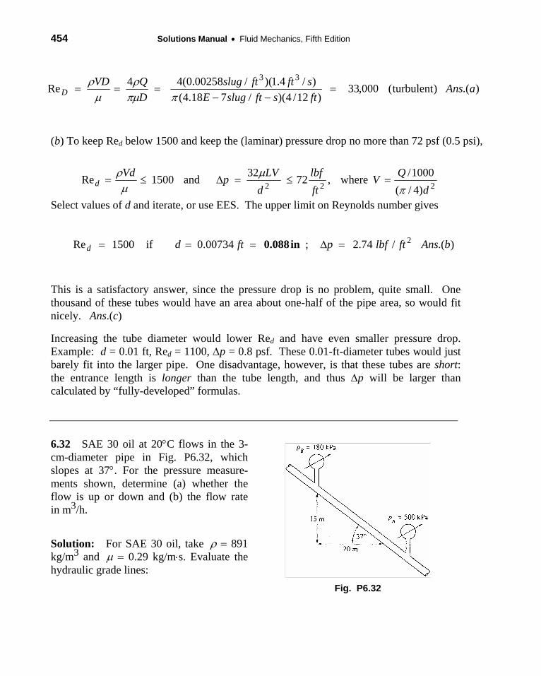
6.30 SAE 10 oil at 20°C flows through the 4-cm-diameter vertical pipe of Fig. P6.30. For the mercury manometer reading h = 42 cm shown, (a) calculate the volume flow rate in m3/h, and (b) state the direction of flow.
Solution: For SAE 10 oil, take ρ = 870 kg/m3 and μ = 0.104 kg/m⋅s. The pressure at the lower point (1) is considerably higher than p2 according to the manometer reading:
Fig. P6.30
1 2 Hg oilp p ( )g h (13550 870)(9.81)(0.42) 52200 Paρ ρ− = − Δ = − ≈
oilp/( g) 52200/[870(9.81)] 6.12 mρΔ = ≈
This is more than 3 m of oil, therefore it must include a friction loss: flow is up. Ans. (b) The energy equation between (1) and (2), with V1 = V2, gives
1 22 1 f f f 4
p p 128 LQz z h , or 6.12 m 3 m h , or: h 3.12 mg gd
μρ πρ−
= − + = + ≈ =
4 3(6.12 3) (870)(9.81)(0.04) mCompute Q 0.00536 (a)128(0.104)(3.0) s
Ans.π−= = ≈
3m19.3h
Check Re 4 Q/( d) 4(870)(0.00536)/[ (0.104)(0.04)] 1430 (OK, laminar flow).ρ πμ π= = ≈
P6.31 A laminar flow element or LFE (Meriam Instrument Co.) measures low gas-flow rates with a bundle of capillary tubes packed inside a large outer tube. Consider oxygen at 20°C and
1 atm flowing at 84 ft3/min in a 4-in-diameter pipe. (a) Is the flow approaching the element turbulent? (b) If there are 1000 capillary tubes, L = 4 in, select a tube diameter to keep Red below 1500 and also to keep the tube pressure drop no greater than 0.5 lbf/in2. (c) Do the tubes selected in part (b) fit nicely within the approach pipe?
Solution: For oxygen at 20°C and 1 atm (Table A.4), take R = 260 m2/(s2K), hence ρ = p/RT =
(101350Pa)/[260(293K)] = 1.33 kg/m3 = 0.00258 slug/ft3. Also read μ = 2.0E-5 kg/m-s = 4.18E-
7 slug/ft-s. Convert Q = 84 ft3/min = 1.4 ft3/s. Then the entry pipe Reynolds number is
454 Solutions Manual • Fluid Mechanics, Fifth Edition
).()turbulent(000,33)12/4)(/718.4(
)/4.1)(/00258.0(44Re33
aAnsftsftslugE
sftftslugDQVD
D =−−
===ππμ
ρμ
ρ
(b) To keep Red below 1500 and keep the (laminar) pressure drop no more than 72 psf (0.5 psi),
222 )4/(1000/where,7232and1500Re
dQV
ftlbf
dLVpVd
dπ
μμ
ρ=≤=Δ≤=
Select values of d and iterate, or use EES. The upper limit on Reynolds number gives
).(/74.2;00734.0if1500Re 2 bAnsftlbfpftdd =Δ=== in0.088
This is a satisfactory answer, since the pressure drop is no problem, quite small. One thousand of these tubes would have an area about one-half of the pipe area, so would fit nicely. Ans.(c)
Increasing the tube diameter would lower Red and have even smaller pressure drop. Example: d = 0.01 ft, Red = 1100, Δp = 0.8 psf. These 0.01-ft-diameter tubes would just barely fit into the larger pipe. One disadvantage, however, is that these tubes are short: the entrance length is longer than the tube length, and thus Δp will be larger than calculated by “fully-developed” formulas.
6.32 SAE 30 oil at 20°C flows in the 3-cm-diameter pipe in Fig. P6.32, which slopes at 37°. For the pressure measure-ments shown, determine (a) whether the flow is up or down and (b) the flow rate in m3/h.
Solution: For SAE 30 oil, take ρ = 891 kg/m3 and μ = 0.29 kg/m⋅s. Evaluate the hydraulic grade lines:
Fig. P6.32
BB B A
p 180000 500000HGL z 15 35.6 m; HGL 0 57.2 mg 891(9.81) 891(9.81)ρ
= + = + = = + =
A BSince HGL HGL the (a)Ans. > flow is up
The head loss is the difference between hydraulic grade levels:
f 4 4128 LQ 128(0.29)(25)Qh 57.2 35.6 21.6 m
gd (891)(9.81)(0.03)μ
πρ π= − = = =
3Solve for Q 0.000518 m /s / (b)Ans.= ≈ 31.86 m h
Finally, check Re = 4ρQ/(πμd) ≈ 68 (OK, laminar flow).
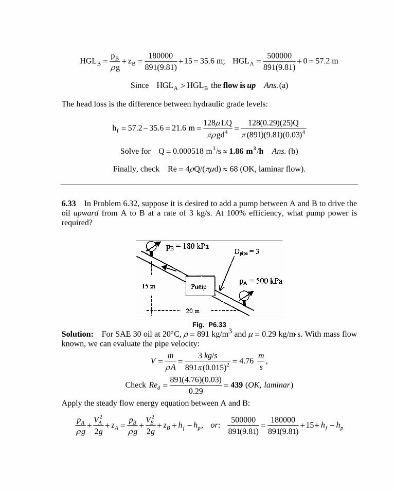
6.33 In Problem 6.32, suppose it is desired to add a pump between A and B to drive the oil upward from A to B at a rate of 3 kg/s. At 100% efficiency, what pump power is required?
Fig. P6.33
Solution: For SAE 30 oil at 20°C, ρ = 891 kg/m3 and μ = 0.29 kg/m⋅s. With mass flow known, we can evaluate the pipe velocity:
2891 (0.015)891(4.76)(0.03)Check ( , )
0.29d
A s3 / 4.76 ,
m kg s mV
Re OK laminar
ρ π
= = 439
= = =
Apply the steady flow energy equation between A and B: 2 2 500000 180000, : 15
2 2 891(9.81) 891(9.81)A A B B
A B f p fp V p Vz z h h or h h
g g g gρ ρ+ + = + + + − = + + − p
456 Solutions Manual • Fluid Mechanics, Fifth Edition
2 232 32(0.29)(25)(4.76)where 140.5 , Solve for 118.9
891(9.81)(0.03)f pumpLVh m
gdμ
ρ= = = =h m
The pump power is then given by
23 9.81 (118.9 )p pkg mgQh mgh m Ans.s s
ρ ⎛ ⎞ ⎛ ⎞= = = =⎜ ⎟ ⎜ ⎟⎝ ⎠ ⎝ ⎠Power 3500 watts
6.34 Derive the time-averaged x-momentum equation (6.21) by direct substitution of Eqs. (6.19) into the momentum equation (6.14). It is convenient to write the convective acceleration as
2u (u ) (uv) (uw)t x y z
dd
∂ ∂ ∂∂ ∂ ∂
= + +
which is valid because of the continuity relation, Eq. (6.14).
Solution: Into the x-momentum eqn. substitute u = u + u’, v = v + v’, etc., to obtain
2 2(u 2uu’ u’ ) (v u vu’ v’u v’u’) (wu wu’ w’u w’u’)∂ ∂ ∂ρ
2x
x y z
(p p’) g [ (u u’)]x
∂ ∂ ∂∂ ρ μ
∂
⎡ ⎤+ + + + + + + + + +⎢ ⎥
⎣ ⎦
= − + + + ∇ +
Now take the time-average of the entire equation to obtain Eq. (6.21) of the text:
.Ans⎡ ⎤⎢ ⎥⎣ ⎦
+ ( ) + ( ) + ( ) = − + + ∇ ( )2 2x
du pu’ u’v’ u’w’ g udt x y z x
∂ ∂ ∂ ∂ρ ρ∂ ∂ ∂ ∂
μ
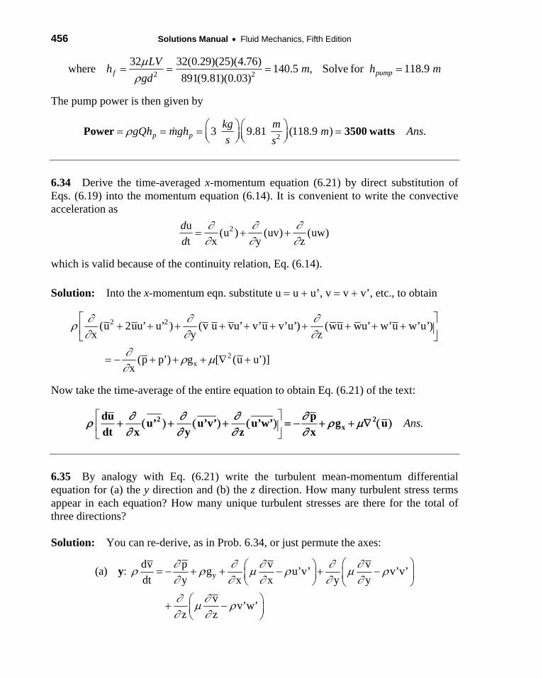
6.35 By analogy with Eq. (6.21) write the turbulent mean-momentum differential equation for (a) the y direction and (b) the z direction. How many turbulent stress terms appear in each equation? How many unique turbulent stresses are there for the total of three directions?
Solution: You can re-derive, as in Prob. 6.34, or just permute the axes:
ydv p v v(a) : g u’v’ v’v’∂ ∂ ∂ ∂ ∂ρ ρ μ ρ μ ρ⎛ ⎞⎛ ⎞= − + + − + −⎜ ⎟ ⎜ ⎟ydt y x x y y
v v’w’z z
∂ ∂ ∂ ∂ ∂
∂ ∂μ ρ∂ ∂
⎝ ⎠ ⎝ ⎠⎛ ⎞+ −⎜ ⎟⎝ ⎠
Chapter 6 • Viscous Flow in Ducts 457
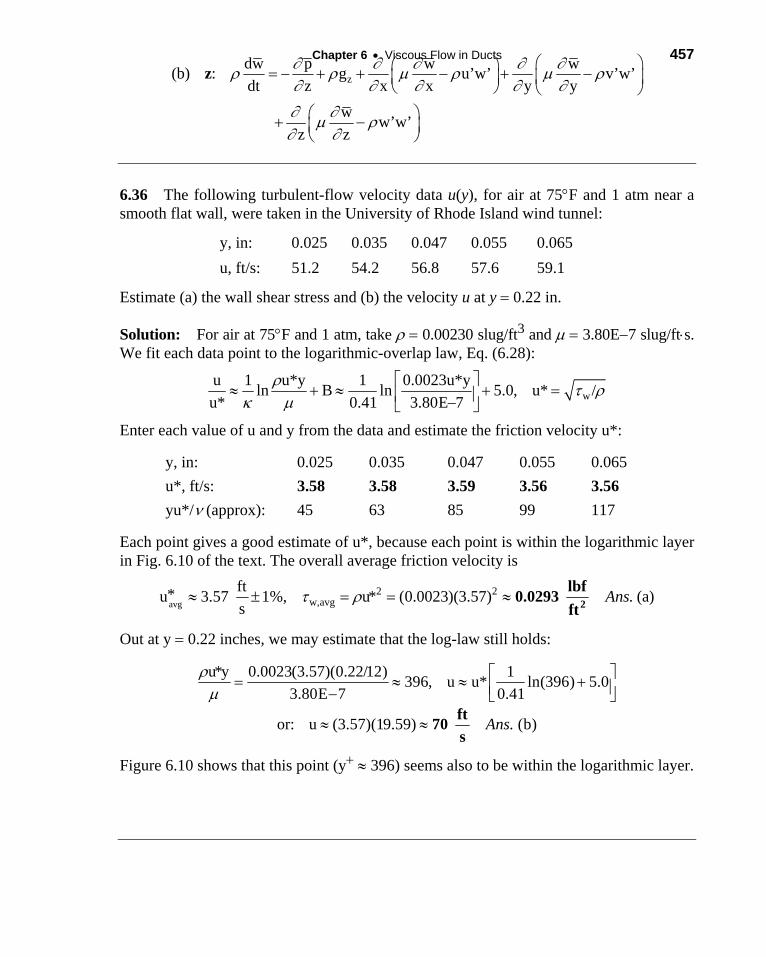
zdw p w w(b) : g u’w’ v’w’∂ ∂ ∂ ∂ ∂ρ ρ μ ρ μ ρ⎛ ⎞⎛ ⎞= − + + − + −⎜ ⎟ ⎜ ⎟zdt z x x y y
w w’w’z z
∂ ∂ ∂ ∂ ∂
∂ ∂μ ρ∂ ∂
⎝ ⎠ ⎝ ⎠⎛ ⎞+ −⎜ ⎟⎝ ⎠
6.36 The following turbulent-flow velocity data u(y), for air at 75°F and 1 atm near a smooth flat wall, were taken in the University of Rhode Island wind tunnel:
y, in: 0.025 0.035 0.047 0.055 0.065 u, ft/s: 51.2 54.2 56.8 57.6 59.1
Estimate (a) the wall shear stress and (b) the velocity u at y = 0.22 in.
Solution: For air at 75°F and 1 atm, take ρ = 0.00230 slug/ft3 and μ = 3.80E−7 slug/ft⋅s. We fit each data point to the logarithmic-overlap law, Eq. (6.28):
wu 1 u*y 1 0.0023u*yln B ln 5.0, u* /u* 0.41 3.80E 7
ρ τ ρκ μ
⎡ ⎤≈ + ≈ + =⎢ ⎥−⎣ ⎦
Enter each value of u and y from the data and estimate the friction velocity u*:
y, in: 0.025 0.035 0.047 0.055 0.065 u*, ft/s: 3.58 3.58 3.59 3.56 3.56 yu*/ν (approx): 45 63 85 99 117
Each point gives a good estimate of u*, because each point is within the logarithmic layer in Fig. 6.10 of the text. The overall average friction velocity is
avg2 2
w,avgft*u 3.57 1%, u* (0.0023)(3.57) (a)s
Ans.τ ρ≈ ± = = ≈ 2lbf0.0293ft
Out at y = 0.22 inches, we may estimate that the log-law still holds:
u*y 0.0023(3.57)(0.22/12) 1396, u u* ln(396) 5.03.80E 7 0.41
ρμ
⎡ ⎤= ≈ ≈ +⎢ ⎥− ⎣ ⎦
or: u (3.57)(19.59) (b)Ans.≈ ≈ft70s
Figure 6.10 shows that this point (y+ ≈ 396) seems also to be within the logarithmic layer.
458 Solutions Manual • Fluid Mechanics, Fifth Edition
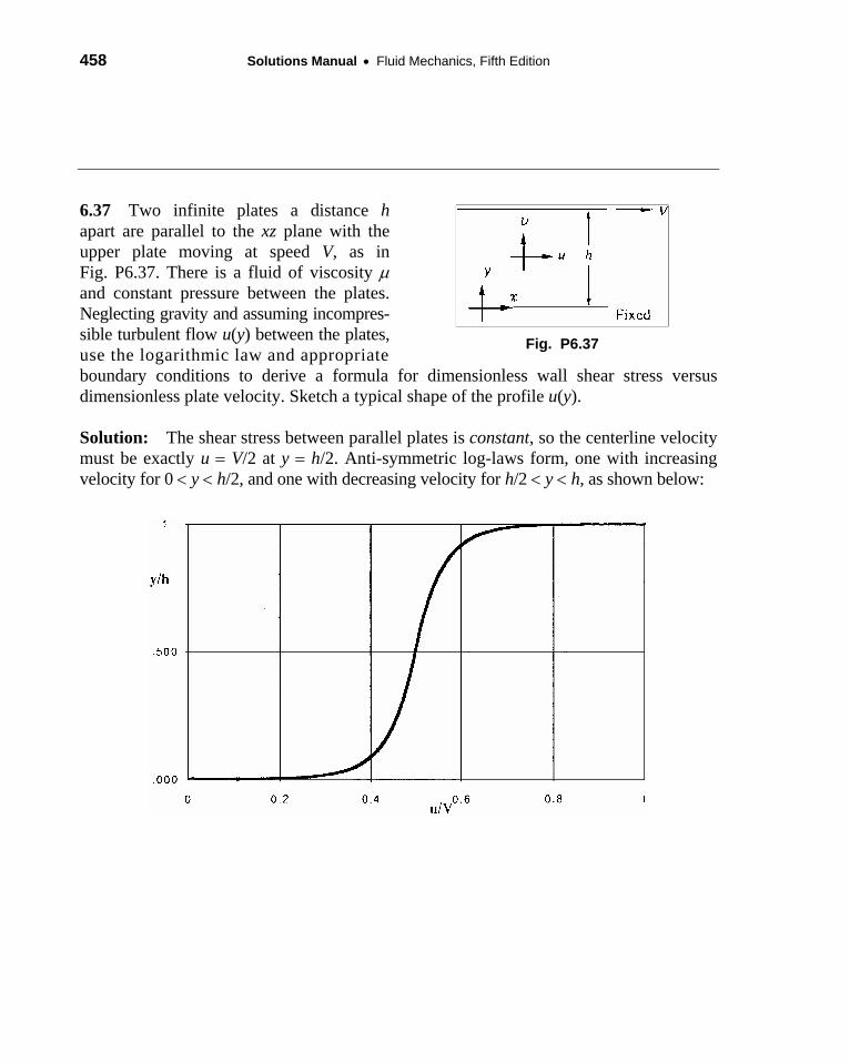
6.37 Two infinite plates a distance h apart are parallel to the xz plane with the upper plate moving at speed V, as in Fig. P6.37. There is a fluid of viscosity μ and constant pressure between the plates. Neglecting gravity and assuming incompres-sible turbulent flow u(y) between the plates, use the logarithmic law and appropriate
Fig. P6.37
boundary conditions to derive a formula for dimensionless wall shear stress versus dimensionless plate velocity. Sketch a typical shape of the profile u(y).
Solution: The shear stress between parallel plates is constant, so the centerline velocity must be exactly u = V/2 at y = h/2. Anti-symmetric log-laws form, one with increasing velocity for 0 < y < h/2, and one with decreasing velocity for h/2 < y < h, as shown below:

Chapter 6 • Viscous Flow in Ducts 459
The match-point at the center gives us a log-law estimate of the shear stress:
1 *ln B, 0.41, B 5.0, 2 * 2V hu Ans.u
κκ ν
⎛ ⎞≈ + ≈ ≈⎜ ⎟⎝ ⎠
u 1 2w* ( ) /= /τ ρ
This is one form of “dimensionless shear stress.” The more normal form is friction coefficient versus Reynolds number. Calculations from the log-law fit a Power-law curve-fit expression in the range 2000 < Reh < 1E5:
w2 1/4
0.018(1/2) ( / )
Ans.V Vh
τρ ρ ν
= ≈ =f 1 4h
0.018CRe /
6.38 Suppose in Fig. P6.37 that h = 3 cm, the fluid is water at 20°C (ρ = 998 kg/m3, μ = 0.001 kg/m⋅s), and the flow is turbulent, so that the logarithmic law is valid. If the shear stress in the fluid is 15 Pa, estimate V in m/s.
Solution: Just as in Prob. 6.37, apply the log-law at the center between the wall, that is, y = h/2, u = V/2. With τw known, we can evaluate u* immediately:
15 /2 1 * /2* 0.123 , ln ,998 *
w m V u hu Bs u
τρ κ
⎛ ⎞ν
= = = ≈ +⎜ ⎟⎝ ⎠
/2 1 0.123(0.03/2)or: ln 5.0 23.3, .0.123 0.41 0.001/998V Solve for Ans⎡ ⎤
= + =⎢ ⎥⎣ ⎦
mV 5.72s
≈
6.39 By analogy with laminar shear, τ = μ du/dy. T. V. Boussinesq in 1877 postulated that turbulent shear could also be related to the mean-velocity gradient τturb = ε du/dy, where ε is called the eddy viscosity and is much larger than μ. If the logarithmic-overlap law, Eq. (6.28), is valid with τ ≈ τw, show that ε ≈ κρu*y.
Solution: Differentiate the log-law, Eq. (6.28), to find du/dy, then introduce the eddy viscosity into the turbulent stress relation:
1 *ln ,*
u yu duIf B thenu d
uy yκ ν κ
∗⎛ ⎞= +⎜ ⎟⎝ ⎠=
2 ** ,wdu uThen, if u solve for Ans.dy y
τ τ ρ ε εκ
≈ ≡ = = ε κρ= u * y

460 Solutions Manual • Fluid Mechanics, Fifth Edition
6.40 Theodore von Kármán in 1930 theorized that turbulent shear could be represented by τ turb = ε du/dy where ε = ρκ 2y2⏐du/dy⏐ is called the mixing-length eddy viscosity and κ ≈ 0.41 is Kármán’s dimensionless mixing-length constant [2,3]. Assuming that τ turb ≈ τw near the wall, show that this expression can be integrated to yield the logarithmic-overlap law, Eq. (6.28).
Solution: This is accomplished by straight substitution:
2 2 2turb w
du du du du u*u* y , solve fordy dy dy dy y
τ τ ρ ε ρκκ
⎡ ⎤≈ = = = =⎢ ⎥
⎣ ⎦
u* dyIntegrate: du , or: .y
Ansκ
=∫ ∫u*u ln(y) constant= +κ
To convert this to the exact form of Eq. (6.28) requires fitting to experimental data. ______________________________________________________________________________________
P6.41 Two reservoirs, which differ in surface elevation by 40 m, are connected by 350 m of new pipe of diameter 8 cm. If the desired flow rate is at least 130 N/s of water at 20°C, may the pipe material be (a) galvanized iron, (b) commercial steel, or (c) cast iron? Neglect minor losses.
Solution: Applying the extended Bernoulli equation between reservoir surfaces yields
)/81.9(2)
08.0350(
240 2
22
smV
mmf
gV
DLfmz ===Δ
where f and V are related by the friction factor relation:
μρε VD
fD
f DD
=+−≈ Rewhere)Re
51.27.3
/(log0.2110
When V is found, the weight flow rate is given by w = ρgQ where Q = AV = (πD2/4)V. For
water at 20°C, take ρ = 998 kg/m3 and μ = 0.001 kg/m-s. Given the desired w = 130 N/s, solve
this system of equations by EES to yield the wall roughness. The results are:

Chapter 6 • Viscous Flow in Ducts 461
f = 0.0257 ; V = 2.64 m/s ; ReD = 211,000 ; εmax = 0.000203 m = 0.203 mm
Any less roughness is OK. From Table 6-1, the three pipe materials have (a) galvanized: ε = 0.15 mm ; (b) commercial steel: ε = 0.046 mm ; cast iron: ε = 0.26 mm
Galvanized and steel are fine, but cast iron is too rough.. Ans. Actual flow rates are
(a) galvanized: 135 N/s; (b) steel: 152 N/s; (c) cast iron: 126 N/s (not enough)
6.42 It is clear by comparing Figs. 6.12b and 6.13 that the effects of sand roughness and commercial (manufactured) roughness are not quite the same. Take the special case of commercial roughness ratio ε/d = 0.001 in Fig. 6.13, and replot in the form of the wall-law shift ΔB (Fig. 6.12a) versus the logarithm of ε+ = εu∗/ν. Compare your plot with Eq. (6.45).
Solution: To make this plot we must relate ΔB to the Moody-chart friction factor. We use Eq. (6.33) of the text, which is valid for any B, in this case, B = Bo − ΔB, where Bo ≈ 5.0:
o dV 1 Ru* 3 V 8 Ru* 1 fln B B , where and Reu* 2 u* f 2 8κ ν κ ν
⎛ ⎞≈ + − Δ − = =⎜ ⎟⎝ ⎠ (1)
Combine Eq. (1) with the Colebrook friction formula (6.48) and the definition of ε+:
101 / 2.512.0 log
3.7f Rdε⎛≈ − +⎜⎝√ √e f
⎞⎟⎠
(2)
u* fand Re8
dd d
ε ε εε
ν+ += = = (3)
Equations (1, 2, 3) enable us to make the plot below of “commercial” log-shift ΔB, which is similar to the ‘sand-grain’ shift predicted by Eq. (6.45): ΔBBsand ≈ (1/κ)ln(ε ) − 3.5. +
Ans.
Fig. P6.42
______________________________________________________________________________________
462 Solutions Manual • Fluid Mechanics, Fifth Edition
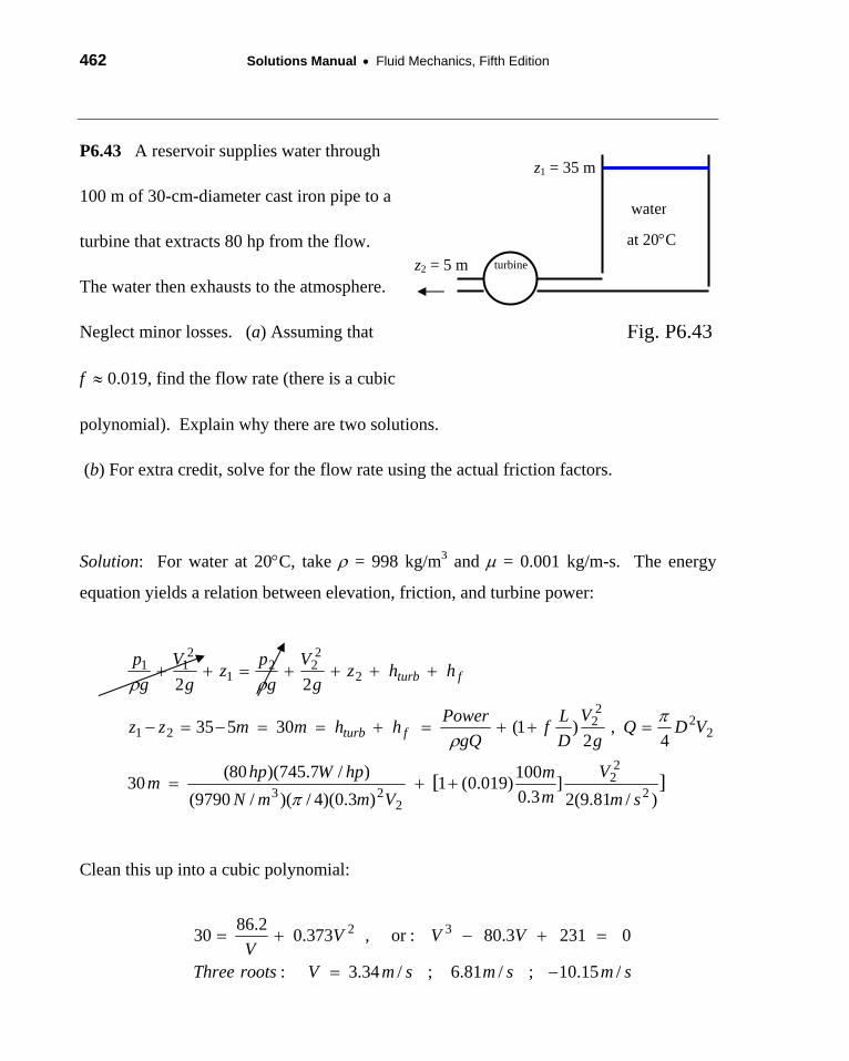
P6.43 A reservoir supplies water through z1 = 35 m
100 m of 30-cm-diameter cast iron pipe to a water
at 20°C turbine that extracts 80 hp from the flow. z2 = 5 m turbine
The water then exhausts to the atmosphere.
Fig. P6.43 Neglect minor losses. (a) Assuming that
f ≈ 0.019, find the flow rate (there is a cubic
polynomial). Explain why there are two solutions.
(b) For extra credit, solve for the flow rate using the actual friction factors.
Solution: For water at 20°C, take ρ = 998 kg/m3 and μ = 0.001 kg/m-s. The energy
equation yields a relation between elevation, friction, and turbine power:
][)/81.9(2
]3.0
100)019.0(1)3.0)(4/)(/9790(
)/7.745)(80(30
4,
2)1(30535
22
2
22
223
22
22
21
2
222
1
211
smV
mm
VmmNhpWhpm
VDQg
VDLf
gQPowerhhmmzz
hhzg
Vg
pzg
Vg
p
fturb
fturb
++=
=++=+==−=−
++++=++
π
πρ
ρρ
Clean this up into a cubic polynomial:
smsmsmVrootsThree
VVVV
/15.10;/81.6;/34.3:
02313.80:or,373.02.8630 32
−=
=+−+=
Chapter 6 • Viscous Flow in Ducts 463
The third (negative) root is meaningless. The other two are correct. Either
Q = 0.481 m3/s , hturbine = 12.7 m , hf = 17.3 m
Q = 0.236 m3/s , hturbine = 25.8 m , hf = 4.2 m Ans.(a)
Both solutions are valid. The higher flow rate wastes a lot of water and creates 17 meters of
friction loss. The lower rate uses 51% less water and has proportionately much less friction.
(b) The actual friction factors are very close to the problem’s “Guess”. Thus we obtain
Re = 2.04E6, f = 0.0191; Q = 0.479 m3/s , hturbine = 12.7 m , hf = 17.3 m
Re = 1.01E6, f = 0.0193 ; Q = 0.237 m3/s , hturbine = 25.7 m , hf = 4.3 m
Ans.(b)
The same remarks apply: The lower flow rate is better, less friction, less water used.
6.44 Mercury at 20°C flows through 4 meters of 7-mm-diameter glass tubing at an average velocity of 5 m/s. Estimate the head loss in meters and the pressure drop in kPa.
Solution: For mercury at 20°C, take ρ = 13550 kg/m3 and μ = 0.00156 kg/m⋅s. Glass tubing is considered hydraulically “smooth,” ε/d = 0. Compute the Reynolds number:
.13550(5)(0 007) 304,000; Moody chart smooth: 0.01430.00156d
Vd fρμ
= = = ≈Re
⎛ ⎞= = =⎜ ⎟⎝ ⎠
10.4 m2 24.0 50.0143 (a)
2 0.007 2(9.81)fL Vh f Ans.d g
(13550)(9.81)(10.4) 1,380,000 (b)fp gh Pa Ans. ρΔ = = = = 1380 kPa
6.45 Oil, SG = 0.88 and ν = 4E−5 m2/s, flows at 400 gal/min through a 6-inch asphalted cast-iron pipe. The pipe is 0.5 miles long (2640 ft) and slopes upward at 8° in the flow direction. Compute the head loss in feet and the pressure change.

464 Solutions Manual • Fluid Mechanics, Fifth Edition
Solution: First convert 400 gal/min = 0.891 ft3/s and ν = 0.000431 ft2/s. For asphalted cast-iron, ε = 0.0004 ft, hence ε/d = 0.0004/0.5 = 0.0008. Compute V, Red, and f:
20.891 4.54(0.5)4.54 ; 5271; calculate 0.0377
0.000431(0.25) d MoodyftV fsπ
= = = = =Re
2 22640 (4.54)then 0.0377 (a)2 0.5 2(32.2)f
L Vh f Ans.d g
⎛ ⎞= = =⎜ ⎟⎝ ⎠63.8 ft
If the pipe slopes upward at 8°, the pressure drop must balance both friction and gravity:
( ) 0.88(62.4)[63.8 2640sin8 ] (b)fp g h z Ans.ρΔ = + Δ = + ° = 2lbf23700ft
6.46 Kerosene at 20°C is pumped at 0.15 m3/s through 20 km of 16-cm-diameter cast-iron horizontal pipe. Compute the input power in kW required if the pumps are 85 percent efficient.
Solution: For kerosene at 20°C, take ρ = 804 kg/m3 and μ = 1.92E−3 kg/m⋅s. For cast iron take ε ≈ 0.26 mm, hence ε/d = 0.26/160 ≈ 0.001625. Compute V, Re, and f:
20.15 m 4 Q 4(804)(0.15)V 7.46 ; Re 500,000
s d (0.00192)(0.16)( /4)(0.16)ρ
πμ ππ= = = = ≈
/ 0.001625: Moody chart: f 0.0226dε ≈ ≈
2 2
fL V 20000 (7.46)Then h f (0.0226) 8020 md 2g 0.16 2(9.81)
⎛ ⎞= = ≈⎜ ⎟⎝ ⎠
At 85% efficiency, the pumping power required is:
fgQh 804(9.81)(0.15)(8020)P 11.2E 6 W0.85
Ans.ρη
= = ≈ + = 11.2 MW

Chapter 6 • Viscous Flow in Ducts 465
6.47 The gutter and smooth drainpipe in Fig. P6.47 remove rainwater from the roof of a building. The smooth drainpipe is 7 cm in diameter. (a) When the gutter is full, estimate the rate of draining. (b) The gutter is designed for a sudden rainstorm of up to 5 inches per hour. For this condition, what is the maximum roof area that can be drained successfully?
Solution: If the velocity at the gutter surface is neglected, the energy equation reduces to
Fig. P6.47
2 2 2)
ns
2 2 2(9.81)(4., , solve2 2 1 / 1 (4.2/0.07)f fV L V g zz h h f V
g d g fL d fΔ
Δ = + = = =+ +
For water, take ρ = 998 kg/m3 and μ = 0.001 kg/m⋅s. Guess f ≈ 0.02 to obtain the velocity estimate V ≈ 6 m/s above. Then Red ≈ ρVd/μ ≈ (998)(6)(0.07)/(0.001) ≈ 428,000 (turbulent). Then, for a smooth pipe, f ≈ 0.0135, and V is changed slightly to 6.74 m/s. After convergence, we obtain
26.77 m/s, ( /4)(0.07) . (a)V Q V Aπ= = = 30.026 m /s
A rainfall of 5 in/h = (5/12 ft/h)(0.3048 m/ft)/(3600 s/h) = 0.0000353 m/s. The required roof area is
3roof drain rain/ (0.026 m /s)/0.0000353 m/s (b)A Q V Ans.= = ≈ 2740 m
6.48 Show that if Eq. (6.33) is accurate, the position in a turbulent pipe flow where local velocity u equals average velocity V occurs exactly at r = 0.777R, independent of the Reynolds number.
Solution: Simply find the log-law position y+ where u+ exactly equals V/u*:
?1 Ru* 3 1 yu* 1 y 3V u* ln B – u* ln B if ln2 R 2κ ν κ κ ν κ
⎡ ⎤ ⎡ ⎤= + = + =⎢ ⎥ ⎢ ⎥⎣ ⎦ ⎣ ⎦ κ−
3/2rSince y R – r, this is equivalent to 1– e 1– 0.223R
Ans.−= = = 0.777≈

6.49 The tank-pipe system of Fig. P6.49 is to deliver at least 11 m3/h of water at 20°C to the reservoir. What is the maximum roughness height ε allowable for the pipe?
Solution: For water at 20°C, take ρ = 998 kg/m3 and μ = 0.001 kg/m⋅s. Evaluate V and Re for the expected flow rate:
Fig. P6.49
2Q 11/3600 m Vd 998(4.32)(0.03)V 4.32 ; Re 129000A s 0.001( /4)(0.03)
ρμπ
= = = = = =
The energy equation yields the value of the head loss: 2 2 2
3.05 matm atm1 21 2 f f
p pV V (4.32)z z h or h 4g 2g g 2g 2(9.81)ρ ρ
+ + = + + + = − =
2 2≈f
L V 5.0 (4.32)But also h f , or: 3.05 f , solve for f 0.0192d 2g 0.03 2(9.81)
⎛ ⎞= = ⎜ ⎟⎝ ⎠
With f and Re known, we can find ε/d from the Moody chart or from Eq. (6.48):
101/2 1/21 / 2.512.0 log , solve for 0.000394
3.7(0.0192) 129000(0.0192)d
dε ε⎡ ⎤
= − + ≈⎢ ⎥⎣ ⎦
Then 0.000394(0.03) 1.2E 5 m (very smooth) Ans.ε = ≈ − ≈ 0.012 mm
6.50 Ethanol at 20°C flows at 125 U.S. gal/min through a horizontal cast-iron pipe with L = 12 m and d = 5 cm. Neglecting entrance effects, estimate (a) the pressure gradient, dp/dx; (b) the wall shear stress, τw; and (c) the percent reduction in friction factor if the pipe walls are polished to a smooth surface.
Solution: For ethanol (Table A-3) take ρ = 789 kg/m3 and μ = 0.0012 kg/m⋅s. Convert 125 gal/min to 0.00789 m3/s. Evaluate V = Q/A = 0.00789/[π (0.05)2/4] = 4.02 m/s.
789(4.02)(0.05) 0.26 132,000, 0.0052 Then 0.03140.0012 50 d Moody
Vd mmRe fd mm
ρ εμ
= = = = = ≈
2 20.0314(b) (789)(4.02) (b)8 8wf V Ans.τ ρ= = = 50 Pa
4 4(50)(a) (a)0.05
wdp Ans.dx d
τ −= − = = −
Pa4000m
Chapter 6 • Viscous Flow in Ducts 467
(c) 132000, 0.0170, hence the reduction in f is
0.01701 (c)0.0314
smoothf
Ans.
= =
⎛ ⎞− =⎜ ⎟⎝ ⎠
Re
46%
6.51 The viscous sublayer (Fig. 6.10) is normally less than 1 percent of the pipe diameter and therefore very difficult to probe with a finite-sized instrument. In an effort to generate a thick sublayer for probing, Pennsylvania State University in 1964 built a pipe with a flow of glycerin. Assume a smooth 12-in-diameter pipe with V = 60 ft/s and glycerin at 20°C. Compute the sublayer thickness in inches and the pumping horsepower required at 75 percent efficiency if L = 40 ft.
Solution: For glycerin at 20°C, take ρ = 2.44 slug/ft3 and μ = 0.0311 slug/ft⋅s. Then
MoodyVd 2.44(60)(1 ft)Re 4710 (barely turbulent!) Smooth: f 0.0380
0.0311ρ
μ= = = ≈
1/21/2 0.0380 ftThen u* V(f/8) 60 4.13
8 s⎛ ⎞= = ≈⎜ ⎟⎝ ⎠
The sublayer thickness is defined by y+ ≈ 5.0 = ρyu*/μ. Thus
sublayer5 5(0.0311)y 0.0154 ftu* (2.44)(4.13)
Ans.μρ
≈ = = ≈ 0.185 inches
With f known, the head loss and the power required can be computed:
2 2
fL V 40 (60)h f (0.0380) 85 ftd 2g 1 2(32.2)
⎛ ⎞= = ≈⎜ ⎟⎝ ⎠
2fgQh 1P (2.44)(32.2) (1) (60) (85) 419000 5500.75
Ans.ρ πη
⎡ ⎤= = = ÷ ≈⎢ ⎥4⎣ ⎦760 hp
6.52 The pipe flow in Fig. P6.52 is driven by pressurized air in the tank. What gage pressure p1 is needed to provide a 20°C water flow rate Q = 60 m3/h?
Solution: For water at 20°C, take ρ = 998 kg/m3 and μ = 0.001 kg/m⋅s. Get V, Re, f:
260/3600 mV 8
s( /4)(0.05)π= = .49 ;

468 Solutions Manual • Fluid Mechanics, Fifth Edition
Fig. P6.52
smooth998(8.49)(0.05)Re 424000; f
0.001= ≈ ≈ 0.0136
Write the energy equation between points (1) (the tank) and (2) (the open jet):
22 2pipe1
f f pipeVp 0 0 L V m10 80 h , where h f and V 8.49
g 2g g 2g d 2g sρ ρ+ + = + + + = =
2(8.49) 170⎡ ⎤1Solve p (998)(9.81) 80 10 1 0.0136
2(9.81) 0.05
Ans.
⎧ ⎫⎛ ⎞= − + +⎨ ⎬⎢ ⎥⎜ ⎟⎝ ⎠⎩ ⎭⎣ ⎦≈ 2.38E6 Pa
[This is a gage pressure (relative to the pressure surrounding the open jet.)]
6.53 In Fig. P6.52 suppose p1 = 700 kPa and the fluid specific gravity is 0.68. If the flow rate is 27 m3/h, estimate the viscosity of the fluid. What fluid in Table A-5 is the likely suspect? Solution: Evaluate ρ = 0.68(998) = 679 kg/m3. Evaluate V = Q/A = (27/3600)/[π (0.025)2] = 3.82 m/s. The energy analysis of the previous problem now has f as the unknown:
2 2 21 700000 (3.82) 17070 1 , solve 0.0136
679(9.81) 2 2 2(9.81) 0.05p V L Vz f f fg g d gρ
⎡ ⎤= = Δ + + = + + =⎢ ⎥⎣ ⎦
679(3.82)(0.05)Smooth pipe: 0.0136, 416000 ,
Solve
df
Ans.
μ
μ
= = =
=
Re
kg0.00031m s⋅
The density and viscosity are close to the likely suspect, gasoline. Ans.
6.54* A swimming pool W by Y by h deep is to be emptied by gravity through the long pipe shown in Fig. P6.54. Assuming an average pipe friction factor fav and neglecting minor losses, derive a formula for the time to empty the tank from an initial level ho.

Chapter 6 • Viscous Flow in Ducts 469
Fig. P6.54
Solution: With no driving pressure and negligible tank surface velocity, the energy equation can be combined with a control-volume mass conservation:
2 22 2, :
2 2 4 1av out pipeV L V or Q A V D
g D g fπ
= =+
( )/av
gh dhh t f WYL D dt
= + = −
We can separate the variables and integrate for time to drain:
( )2
0
2 0 24 1 /
o
oav h
g dhD dt WY WYf L D h
π= − = − −
+ ∫ ∫0t
h
:Clean this up to obtain Ans.o avdrain
h f L DWY tgD
+ /≈ 2
2 (1 )4π
1/2
470 Solutions Manual • Fluid Mechanics, Fifth Edition
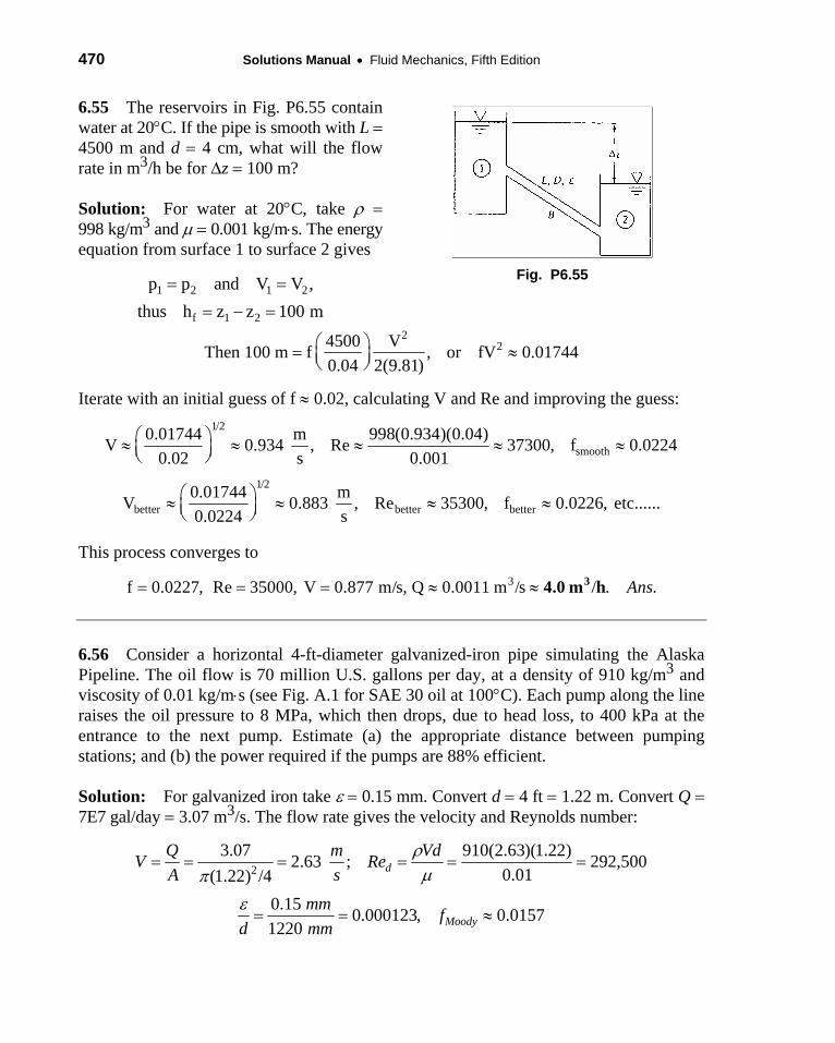
6.55 The reservoirs in Fig. P6.55 contain water at 20°C. If the pipe is smooth with L = 4500 m and d = 4 cm, what will the flow rate in m3/h be for Δz = 100 m?
Solution: For water at 20°C, take ρ = 998 kg/m3 and μ = 0.001 kg/m⋅s. The energy equation from surface 1 to surface 2 gives
1 2 1 2p p and V V= = ,
f 1 2thus h z z 100 m= − =
Fig. P6.55
224500 VThen 100 m f , or fV 0.01744
0.04 2(9.81)⎛ ⎞= ≈⎜ ⎟⎝ ⎠
Iterate with an initial guess of f ≈ 0.02, calculating V and Re and improving the guess: 1/2
smooth0.01744 m 998(0.934)(0.04)V 0.934 , Re 37300, f 0.0224
0.02 s 0.001⎛ ⎞≈ ≈ ≈ ≈ ≈⎜ ⎟⎝ ⎠
1/2
better better better0.01744 mV 0.883 , Re 35300, f 0.0226, etc......0.0224 s
⎛ ⎞≈ ≈ ≈ ≈⎜ ⎟⎝ ⎠
This process converges to 3f 0.0227, Re 35000, V 0.877 m/s, Q 0.0011 m /s / . Ans.= = = ≈ ≈ 34.0 m h
6.56 Consider a horizontal 4-ft-diameter galvanized-iron pipe simulating the Alaska Pipeline. The oil flow is 70 million U.S. gallons per day, at a density of 910 kg/m3 and viscosity of 0.01 kg/m⋅s (see Fig. A.1 for SAE 30 oil at 100°C). Each pump along the line raises the oil pressure to 8 MPa, which then drops, due to head loss, to 400 kPa at the entrance to the next pump. Estimate (a) the appropriate distance between pumping stations; and (b) the power required if the pumps are 88% efficient.
Solution: For galvanized iron take ε = 0.15 mm. Convert d = 4 ft = 1.22 m. Convert Q = 7E7 gal/day = 3.07 m3/s. The flow rate gives the velocity and Reynolds number:
23.07 910(2.63)(1.22)2.63 ; 292,500
0.01(1.22) /4 dQ m VdVA s
ρμπ
= = = = = =Re
0.15 0.000123, 0.01571220 Moody
mm fd mmε
= = ≈

Chapter 6 • Viscous Flow in Ducts 471
Relating the known pressure drop to friction factor yields the unknown pipe length:
9102
2 28,000,00 400,000 0.0157 (2.63) ,2 1.22
L Lp Pa f Vd
ρ ⎛ ⎞Δ = − = = ⎜ ⎟⎝ ⎠
Solve 117 miles (a)L Ans.= =188, 000 m
The pumping power required follows from the pressure drop and flow rate:
3.07(8 6 4 5)Q p E EΔ − 2.65 7 watts0.88
(35,500 hp) (b)
Power EEfficiency
Ans.
= = =
= 26.5 MW
6.57 Apply the analysis of Prob. 6.54 to the following data. Let W = 5 m, Y = 8 m, ho = 2 m, L = 15 m, D = 5 cm, and ε = 0. (a) By letting h = 1.5 m and 0.5 m as representative depths, estimate the average friction factor. Then (b) estimate the time to drain the pool.
Solution: For water, take ρ = 998 kg/m3 and μ = 0.001 kg/m⋅s. The velocity in Prob. 6.54 is calculated from the energy equation:
2 with (Re ) and Re , / 3001 / D smooth pipe D
gh VDV f fcnfL D
ρμ
= = =+
L D =
(a) With a bit of iteration for the Moody chart, we obtain ReD = 108,000 and f ≈ 0.0177 at h = 1.5 m, and ReD = 59,000 and f ≈ .0202 at h = 0.5 m; thus the average value fav ≈ 0.019. Ans. (a)
The drain formula from Prob. 6.54 then predicts:
2 2 9.81(0.05)
33700 (b)
draintgD
s Ans.
π π≈ ≈
= = 9.4 h
2 (1 / )4 4(5)(8) 2(2)[1 0.019(300)]o avh f L DWY + +
6.58 In Fig. P6.55 assume that the pipe is cast iron with L = 550 m, d = 7 cm, and Δz = 100 m. If an 80 percent efficient pump is placed at point B, what input power is required to deliver 160 m3/h of water upward from reservoir 2 to 1?
Fig. P6.55
472 Solutions Manual • Fluid Mechanics, Fifth Edition
Solution: For water at 20°C, take ρ = 998 kg/m3 and μ = 0.001 kg/m⋅s. Compute V, Re:
2Q 160/3600 m 998(11.55)(0.07)V 11.55 ; Re 807000= = ≈ = ≈
cast iron
A s 0.001( /4)(0.07)0.26 mm 0.00371; Moody chart: f 0.0028070 mmd
πε
= ≈ ≈|
The energy equation from surface 1 to surface 2, with a pump at B, gives 2
pump f550 (11.55)h z h 100 (0.0280) 100 1494 1594 m0.07 2(9.81)
⎛ ⎞= Δ + = + = + ≈⎜ ⎟⎝ ⎠
pgQh (998)(9.81)(160/3600)(1594)Power 8.67E5 W0.80
Ans.ρ
η= = = ≈ 867 kW
6.59 The following data were obtained for flow of 20°C water at 20 m3/hr through a badly corroded 5-cm-diameter pipe which slopes downward at an angle of 8°: p1 = 420 kPa, z1 = 12 m, p2 = 250 kPa, z2 = 3 m. Estimate (a) the roughness ratio of the pipe; and (b) the percent change in head loss if the pipe were smooth and the flow rate the same.
Solution: The pipe length is given indirectly as L = Δz/sinθ = (9 m)/sin8° = 64.7 m. The steady flow energy equation then gives the head loss:
2 22 2
1 221 1 420000 250000, : 12 3 ,
2 9790 9790Solve 26.4
f f
f
p V h or hg g
h m
+ + + = + +
=
p Vz zg gρ ρ
= + + +
Now relate the head loss to the Moody friction factor: 2 264.7 (2.83)26.4 , Solve 0.050, 141000, Read 0.0211
2 0.05 2(9.81)fL Vh f f f Red g d
ε= = = = = ≈
The estimated (and uncertain) pipe roughness is thus ε = 0.0211d ≈ 1.06 mm Ans. (a) (b) At the same Red = 141000, fsmooth = 0.0168, or 66% less head loss. Ans. (b)
P6.60 In the spirit of Haaland’s explicit pipe friction factor approximation, Eq. (6.49), Jeppson
[20] proposed the following explicit formula:
)( 9.010Re
74.57.3
/log0.21 df
+−≈d
ε
Chapter 6 • Viscous Flow in Ducts 473
(a) Is this identical to Haaland’s formula and just a simple rearrangement? Explain.
(b) Compare Jeppson to Haaland for a few representative values of (turbulent) Red and
ε/d and their deviations compared to the Colebrook formula (6.48).
Solution: (a) No, it looks like a rearrangement of Haaland’s formula, but it is not. Haaland started with Colebrook’s smooth-wall formula and added just enough ε/d effect for accuracy. Jeppson started with the rough-wall formula and added just enough Red effect for accuracy. Both are excellent approximations over the full (turbulent) range of Red and ε/d. Their predicted values of f are nearly the same and very close to the implicit Colebrook formula. Here is a table of their standard deviations of their values when subtracted from Colebrook:
1E4 < Red < 1e8 ε/d = 0.03 0.01 0.001 0.0001 0.00001
Jeppson rms error 0.000398 0.000328 0.000195 0.000067 0.000088
Haaland rms error 0.000034 0.000043 0.000129 0.000113 0.000083
As expected, Jeppson is slightly better for smooth walls, Haaland for rough walls. Both
are within ±2% of the Colebrook formula over the entire range of Red and ε/d.
6.61 What level h must be maintained in Fig. P6.61 to deliver a flow rate of 0.015 ft3/s through the 1
2 -in commercial-steel pipe?
Fig. P6.61
474 Solutions Manual • Fluid Mechanics, Fifth Edition
Solution: For water at 20°C, take ρ = 1.94 slug/ft3 and μ = 2.09E−5 slug/ft⋅s. For commercial steel, take ε ≈ 0.00015 ft, or ε/d = 0.00015/(0.5/12) ≈ 0.0036. Compute
2Q 0.015 ftV 11.0 ;A s( /4)(0.5/12)π
= = =
MoodyVd 1.94(11.0)(0.5/12)Re 42500 / 0.0036, f 0.0301
2.09E 5dρ ε
μ= = ≈ = ≈
−
The energy equation, with p1 = p2 and V1 ≈ 0, yields an expression for surface elevation: 2 2 2
fV V L (11.0) 80h h 1 f 1 0.03012g 2g d 2(32.2) 0.5/12
Ans.⎡ ⎤⎛ ⎞⎛ ⎞= + = + = + ≈⎜ ⎟ ⎢ ⎥⎜ ⎟⎝ ⎠ ⎝ ⎠⎣ ⎦
111 ft
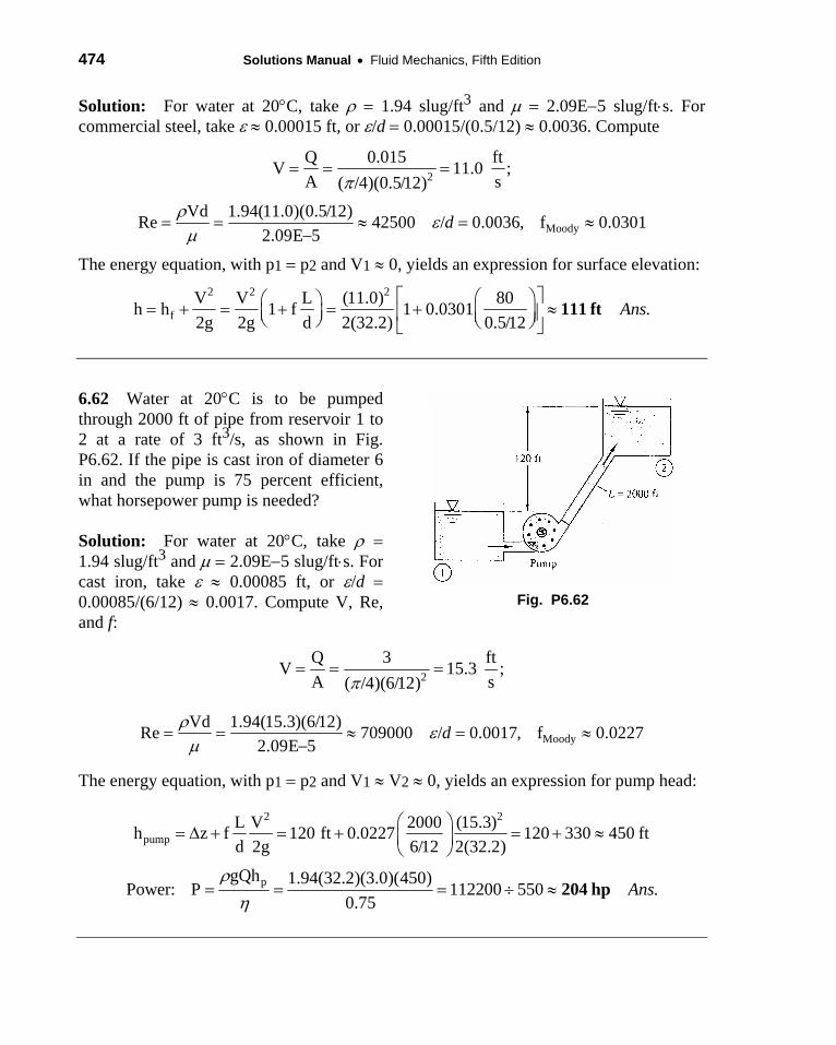
6.62 Water at 20°C is to be pumped through 2000 ft of pipe from reservoir 1 to 2 at a rate of 3 ft3/s, as shown in Fig. P6.62. If the pipe is cast iron of diameter 6 in and the pump is 75 percent efficient, what horsepower pump is needed?
Solution: For water at 20°C, take ρ = 1.94 slug/ft3 and μ = 2.09E−5 slug/ft⋅s. For cast iron, take ε ≈ 0.00085 ft, or ε/d = 0.00085/(6/12) ≈ 0.0017. Compute V, Re, and f:
Fig. P6.62
2Q 3V 15.3 ;A s( /4)(6/12)π
= = =ft
MoodyVd 1.94(15.3)(6/12)Re 709000 / 0.0017, f 0.0227
2.09E 5dρ ε
μ= = ≈ = ≈
−
The energy equation, with p1 = p2 and V1 ≈ V2 ≈ 0, yields an expression for pump head:
2 2
pumpL V 2000 (15.3)h z f 120 ft 0.0227 120 330 450 ftd 2g 6/12 2(32.2)
⎛ ⎞= Δ + = + = + ≈⎜ ⎟
⎝ ⎠
pgQh 1.94(32.2)(3.0)(450)Power: P 112200 5500.75
Ans.ρ
η= = = ÷ ≈ 204 hp
Chapter 6 • Viscous Flow in Ducts 475
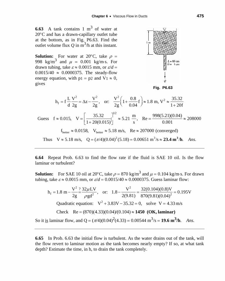
6.63 A tank contains 1 m3 of water at 20°C and has a drawn-capillary outlet tube at the bottom, as in Fig. P6.63. Find the outlet volume flux Q in m3/h at this instant.
Solution: For water at 20°C, take ρ = 998 kg/m3 and μ = 0.001 kg/m⋅s. For drawn tubing, take ε ≈ 0.0015 mm, or ε/d = 0.0015/40 ≈ 0.0000375. The steady-flow energy equation, with p1 = p2 and V1 ≈ 0, gives
Fig. P6.63
2 2 22
fL V V V 0.8 35.32h f z , or: 1 f 1.8 m, Vd 2g 2g 2g 0.04 1 20f
⎛ ⎞= = Δ − + ≈ ≈⎜ ⎟⎝ ⎠ +
1/235.32 m 998(5.21)(0.04)⎡ ⎤
better better
Guess f 0.015, V 5.21 , Re 2080001 20(0.015) s 0.001
f 0.0158, V 5.18 m/s, Re 207000 (converged)
≈ = ≈ = ≈⎢ ⎥+⎣ ⎦
≈ ≈ ≈
2 3Thus V 5.18 m/s, Q ( /4)(0.04) (5.18) 0.00651 m /s / . Ans.π≈ = = ≈ 323.4 m h
6.64 Repeat Prob. 6.63 to find the flow rate if the fluid is SAE 10 oil. Is the flow laminar or turbulent?
Solution: For SAE 10 oil at 20°C, take ρ = 870 kg/m3 and μ = 0.104 kg/m⋅s. For drawn tubing, take ε ≈ 0.0015 mm, or ε/d = 0.0015/40 ≈ 0.0000375. Guess laminar flow:
2 2
2
f 2 2
?V 32 LV V 32(0.104)(0.8)Vh 1.8 m , or: 1.8 0.195V2g 2(9.81)gd 870(9.81)(0.04)
μρ
= − = − = =
Quadratic equation: V 3.83V 35.32 0, solve V 4.33 m/s
Check Re (870)(4.33)(0.04)/(0.104)
+ − = =
= ≈ 1450 (OK, laminar)
So it is laminar flow, and Q = (π/4)(0.04)2(4.33) = 0.00544 m3/s = 19.6 m3/h. Ans.
6.65 In Prob. 6.63 the initial flow is turbulent. As the water drains out of the tank, will the flow revert to laminar motion as the tank becomes nearly empty? If so, at what tank depth? Estimate the time, in h, to drain the tank completely.
476 Solutions Manual • Fluid Mechanics, Fifth Edition
Solution: Recall that ρ = 998 kg/m3, μ = 0.001 kg/m⋅s, and ε/d ≈ 0.0000375. Let Z be the depth of water in the tank (Z = 1 m in Fig. P6.63). When Z = 0, find the flow rate:
2f
2(9.81)(0.8)Z 0, h 0.8 m, V converges to f 0.0171, Re 1360001 20f
= = ≈ = =+
3V 3.42 m/s, Q 12.2 m /h (Z 0)≈ ≈ =
So even when the tank is empty, the flow is still turbulent. Ans.
The time to drain the tank is 2tank tank
d d dZ( ) Q (A Z) (1 m ) Qdt dt dt
υ ,= − = = = −
0m
drainavg1m
dZ 1or t (1 m)Q Q
⎛ ⎞= − = ⎜ ⎟⎝ ⎠∫
So all we need is the average value of (1/Q) during the draining period. We know Q at Z = 0 and Z = 1 m, let’s check it also at Z = 0.5 m: Calculate Qmidway ≈ 19.8 m3/h. Then
⎡ ⎤≈ + + ≈ = ≈⎢ ⎥⎣ ⎦|avg drain3
1 1 1 4 1 h0.0544 , t Q 6 23.4 19.8 12.2 m
Ans.0.0544 h 3.3 min
6.66 Ethyl alcohol at 20°C flows through a 10-cm horizontal drawn tube 100 m long. The fully developed wall shear stress is 14 Pa. Estimate (a) the pressure drop, (b) the volume flow rate, and (c) the velocity u at r = 1 cm.
Solution: For ethyl alcohol at 20°C, ρ = 789 kg/m3, μ = 0.0012 kg/m⋅s. For drawn tubing, take ε ≈ 0.0015 mm, or ε/d = 0.0015/100 ≈ 0.000015. From Eq. (6.12),
wL 100p 4 4(14) (a)d 0.1
Ans.τ ⎛ ⎞Δ = = ≈⎜ ⎟⎝ ⎠
56000 Pa
The wall shear is directly related to f, and we may iterate to find V and Q:
2 2w
f 8(14)V , or: fV 0.142 with 0.0000158 789 d
ετ ρ= = = =
1/20.142 m 789(3.08)(0.1)⎡ ⎤
better better better
Guess f 0.015, V 3.08 , Re 2020000.015 s 0.0012
f 0.0158, V 3.00 m/s, Re 197000 (converged)
≈ = ≈ = ≈⎢ ⎥⎣ ⎦
≈ ≈ ≈
Chapter 6 • Viscous Flow in Ducts 477
Then V ≈ 3.00 m/s, and Q = (π/4)(0.1)2(3.00) = 0.0236 m3/s = 85 m3/h. Ans. (b) Finally, the log-law Eq. (6.28) can estimate the velocity at r = 1 cm, “y” = R − r = 4 cm:
1/2 1/2w 14 mu* 0.133 ;
789 sτρ
⎛ ⎞ ⎛ ⎞= = =⎜ ⎟⎜ ⎟ ⎝ ⎠⎝ ⎠
u 1 u*y 1 789(0.133)(0.04)ln B ln 5.0 24.9u* 0.41 0.0012
ρκ μ
⎡ ⎤ ⎡ ⎤≈ + = +⎢ ⎥ ⎢ ⎥⎣ ⎦⎣ ⎦=
Then u 24.9(0.133) / at r 1 cm. (c)Ans.≈ ≈ =3.3 m s
6.67 A straight 10-cm commercial-steel pipe is 1 km long and is laid on a constant slope of 5°. Water at 20°C flows downward, due to gravity only. Estimate the flow rate in m3/h. What happens if the pipe length is 2 km?
Solution: For water at 20°C, take ρ = 998 kg/m3 and μ = 0.001 kg/m⋅s. If the flow is due to gravity only, then the head loss exactly balances the elevation change:
22
fL Vh z Lsin f , or fV 2gdsin 2(9.81)(0.1)sin 5 0.171d 2g
θ θ= Δ = = = = ° ≈
Thus the flow rate is independent of the pipe length L if laid on a constant slope. Ans. For commercial steel, take ε ≈ 0.046 mm, or ε/d ≈ 0.00046. Begin by guessing fully-rough flow for the friction factor, and iterate V and Re and f:
1/20.171 m 998(3.23)(0.1)f 0.0164, V 3.23 , Re 3220000.0164 s 0.001
⎛ ⎞≈ ≈ ≈ = ≈⎜ ⎟⎝ ⎠
better betterf 0.0179, V 3.09 m/s, Re 308000 (converged)≈ ≈ ≈ 2 3Then Q ( /4)(0.1) (3.09) 0.0243 m /s / . Ans.π≈ ≈ ≈ 387 m h
6.68 The Moody chart, Fig. 6.13, is best for finding head loss (or Δp) when Q, V, d, and L are known. It is awkward for the “2nd” type of problem, finding Q when hf or Δp are known (see Ex. 6.9). Prepare a modified Moody chart whose abscissa is independent of Q and V, using ε/d as a parameter, from which one can immediately read the ordinate to find (dimensionless) Q or V. Use your chart to solve Example 6.9.
Solution: This problem was mentioned analytically in the text as Eq. (6.51). The proper parameter which contains head loss only, and not flow rate, is ζ:
3
1/22
/ 1.775(8 ) log3.7
fd
gd h dReL
εζ ζν ζ
⎛ ⎞= = − +⎜⎝ ⎠⎟
Eq. (6.51)

478 Solutions Manual • Fluid Mechanics, Fifth Edition
We simply plot Reynolds number versus ζ for various ε/d, as shown below:
To solve Example 6.9, a 100-m-long, 30-cm-diameter pipe with a head loss of 8 m and ε/d = 0.0002, we use that data to compute ζ = 5.3E7. The oil properties are ρ = 950 kg/m3 and ν = 2E−5 m2/s. Enter the chart above: let’s face it, the scale is very hard to read, but we estimate, at ζ = 5.3E7, that 6E4 < Red < 9E4, which translates to a flow rate of 0.28 < Q < 0.42 m3/s. Ans. (Example 6.9 gave Q = 0.342 m3/s.)
6.69 For Prob. 6.62 suppose the only pump available can deliver only 80 hp to the fluid. What is the proper pipe size in inches to maintain the 3 ft3/s flow rate?
Solution: For water at 20°C, take ρ = 1.94 slug/ft3 and μ = 2.09E−5 slug/ft⋅s. For cast iron, take ε ≈ 0.00085 ft. We can’t specify ε/d because we don’t know d. The energy analysis above is correct and should be modified to replace V by Q:
2 2 2 2
p 5L (4Q/ d ) 2000 [4(3.0)/ d ] fh 120 f 120 f 120 453d 2g d 2(32.2) d
π π= + = + = +
p 5Power 80(550) 453 fBut also h 235 120 , or:
gQ 62.4(3.0) dρ= = = = + 5d 3.94f≈
Chapter 6 • Viscous Flow in Ducts 479
Guess f ≈ 0.02, calculate d, ε/d and Re and get a better f and iterate:
1/5 4 Q 4(1.94)(3.0)f 0.020, d [3.94(0.02)] 0.602 ft, Re ,d (2.09E 5)(0.602)
ρπμ π
≈ ≈ ≈ = =−
better0.00085or Re 589000, 0.00141, Moody chart: f 0.0218 (repeat)0.602d
ε≈ = ≈ ≈
We are nearly converged. The final solution is f ≈ 0.0217, d ≈ 0.612 ft ≈ 7.3 in Ans.
P6.70 Water at 68°F flows through 200 ft of a horizontal 6-in-diameter asphalted cast iron pipe. (a) If the head loss is 4.5 ft, find the average velocity and the flow rate, using the rescaled variable ζ discussed as a “Type 2” problem. (b) Does this input data seem familiar to you?
Solution: For water in BG units, take ν = 1.1E-5 ft2/s. For asphalted cast iron, ε = 0.0004 ft, hence ε/d = 0.0004ft/0.5ft = 0.0008. Calculate the velocity-free group ζ :
8485.7)/51.1)(200(
)5.4()5.0)(/2.32(2
32
2
3
EsftEft
ftftsftL
hdg f =−
==ν
ζ
Now get the Reynolds number from the modified Colebrook formula, Eq. (6.51):
).(/19.1)/05.6()5.0(44
).(/05.65.0
)274800)(51.1(ReThen
800,274]8485.7
775.17.3
0008.0[log]8485.78[775.17.3
/log)8(Re
322
10102/1 )(
aAnssftsftftVdQ
aAnssftEd
V
EEd
d
d
===
=−
==
=+−=+−=
ππ
νζ
εζ
(b) These are the numbers for L. F. Moody’s classic example, which was introduced in
Ex. 6.6 of the text. We did not get V = 6.00 ft/s because hf was rounded off from 4.47 ft.

480 Solutions Manual • Fluid Mechanics, Fifth Edition
6.71 It is desired to solve Prob. 6.62 for the most economical pump and cast-iron pipe system. If the pump costs $125 per horsepower delivered to the fluid and the pipe costs $7000 per inch of diameter, what are the minimum cost and the pipe and pump size to maintain the 3 ft3/s flow rate? Make some simplifying assumptions.
Solution: For water at 20°C, take ρ = 1.94 slug/ft3 and μ = 2.09E−5 slug/ft⋅s. For cast iron, take ε ≈ 0.00085 ft. Write the energy equation (from Prob. 6.62) in terms of Q and d:
2 2
5
in hp f 5gQ 62.4(3.0) 2000 [4(3.0)/ d ] 154.2fP ( z h ) 120 f 40.84
550 550 d 2(32.2) dρ π⎧ ⎫⎛ ⎞= Δ + = + = +⎨ ⎬⎜ ⎟⎝ ⎠ ⎪⎩ ⎭
hp inches
5
Cost $125P $7000d 125(40.84 154.2f/d ) 7000(12d), with d in ft.
Clean up: Cost $5105 19278f/d 84000d
= + = + +
≈ + +
Regardless of the (unknown) value of f, this Cost relation does show a minimum. If we assume for simplicity that f is constant, we may use the differential calculus:
1/6f const best6
d(Cost) 5(19278)f 84000, or d (1.148 f)d( ) dd ≈
−= + ≈|
1/6 4 Q
better better
Guess f 0.02, d [1.148(0.02)] 0.533 ft, Re 665000, 0.00159d d
Then f 0.0224, d 0.543 ft (converged)
ρ ε≈ ≈ ≈ = ≈ ≈
πμ
≈ ≈
Result: dbest ≈ 0.543 ft ≈ 6.5 in, Costmin ≈ $14300pump + $45600pipe ≈ $60000. Ans.
6.72 Modify Prob. P6.57 by letting the diameter be unknown. Find the proper pipe diameter for which the pool will drain in about 2 hours flat.
Solution: Recall the data: Let W = 5 m, Y = 8 m, ho = 2 m, L = 15 m, and ε = 0, with water, ρ = 998 kg/m3 and μ = 0.001 kg/m⋅s. We apply the same theory as Prob. 6.57:
22 (1 / )2 4, , (Re ) for a smooth pipe.
1 /o av
drain av Dh f L Dgh WYV t f fcn
fL D gDπ+
= ≈ =+
For the present problem, tdrain = 2 hours and D is the unknown. Use an average value h = 1 m to find fav. Enter these equations on EES (or you can iterate by hand) and the final results are
av2.36 m/s; Re 217,000; 0.0154; 0.092 mDV f D= = ≈ = ≈ 9.2 cm Ans.
Chapter 6 • Viscous Flow in Ducts 481
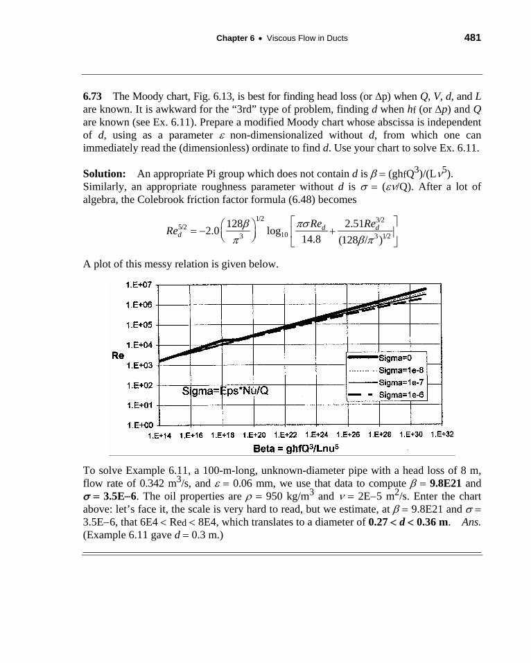
6.73 The Moody chart, Fig. 6.13, is best for finding head loss (or Δp) when Q, V, d, and L are known. It is awkward for the “3rd” type of problem, finding d when hf (or Δp) and Q are known (see Ex. 6.11). Prepare a modified Moody chart whose abscissa is independent of d, using as a parameter ε non-dimensionalized without d, from which one can immediately read the (dimensionless) ordinate to find d. Use your chart to solve Ex. 6.11.
Solution: An appropriate Pi group which does not contain d is β = (ghfQ3)/(Lν5). Similarly, an appropriate roughness parameter without d is σ = (εν/Q). After a lot of algebra, the Colebrook friction factor formula (6.48) becomes
1/2 3/2
1/2π5/2
103 32.511282.0 log
14.8 (128 / )d d
dRe ReRe πσβ
π β⎡ ⎤⎛ ⎞= − +⎢ ⎥⎜ ⎟⎝ ⎠ ⎣ ⎦
A plot of this messy relation is given below.
To solve Example 6.11, a 100-m-long, unknown-diameter pipe with a head loss of 8 m, flow rate of 0.342 m3/s, and ε = 0.06 mm, we use that data to compute β = 9.8E21 and σ = 3.5E−6. The oil properties are ρ = 950 kg/m3 and ν = 2E−5 m2/s. Enter the chart above: let’s face it, the scale is very hard to read, but we estimate, at β = 9.8E21 and σ = 3.5E−6, that 6E4 < Red < 8E4, which translates to a diameter of 0.27 < d < 0.36 m. Ans. (Example 6.11 gave d = 0.3 m.) ________________________________________________________________________
482 Solutions Manual • Fluid Mechanics, Fifth Edition
P6.74 Two reservoirs, which differ in surface elevation by 40 m, are connected by a new commercial steel pipe of diameter 8 cm. If the desired weight flow rate is 200 N/s of water at 20°C, what is the proper length of the pipe? Neglect minor losses.
Solution: For water at 20°C, take ρ = 998 kg/m3 and μ = 0.001 kg/m-s. For commercial steel, ε = 0.046 mm, thus ε/d = 0.046mm/80mm = 0.000575. Find the velocity and the friction factor:
0185.0yields)Re
51.27.3
/(log0.21
000,324001.0
)08.0)(06.4(998Re,06.4)08.0)(4/(
)]81.9(998/[200)4/(
)/(
10
22
=+−≈
======
ff
Df
VDsm
DgwV
D
D
ε
μρ
ππρ
Then we find the pipe length from the energy equation, which is simple in this case:
.205,)81.9(2
)06.4()08.0(
)0185.0(2
4022
AnsmLSolvem
Lg
VDLfmz ≈===Δ

Chapter 6 • Viscous Flow in Ducts 483
6.75 You wish to water your garden with 100 ft of 5
8 -in-diameter hose whose rough-ness is 0.011 in. What will be the delivery, in ft3/s, if the gage pressure at the faucet is 60 lbf/in2? If there is no nozzle (just an open hose exit), what is the maximum horizontal distance the exit jet will carry?
Fig. P6.75
Solution: For water, take ρ = 1.94 slug/ft3 and μ = 2.09E−5 slug/ft⋅s. We are given ε/d = 0.011/(5/8) ≈ 0.0176. For constant area hose, V1 = V2 and energy yields
2 2faucet
fp 60 144 psf L V 100 Vh , or: 138 ft f f ,
g 1.94(32.2) d 2g (5/8)/12 2(32.2)ρ×
= = = =
2fully rough
ftor fV 4.64. Guess f f 0.0463, V 10.0 , Re 48400s
≈ ≈ = ≈ ≈
better finalthen f 0.0472, V (converged)≈ ≈ 9.91 ft/s
The hose delivery then is Q = (π/4)(5/8/12)2(9.91) = 0.0211 ft3/s. Ans. (a) From elementary particle-trajectory theory, the maximum horizontal distance X travelled by the jet occurs at θ = 45° (see figure) and is X = V2/g = (9.91)2/(32.2) ≈ 3.05 ft Ans. (b), which is pitiful. You need a nozzle on the hose to increase the exit velocity.
6.76 The small turbine in Fig. P6.76 extracts 400 W of power from the water flow. Both pipes are wrought iron. Compute the flow rate Q m3/h. Sketch the EGL and HGL accurately.
Solution: For water, take ρ = 998 kg/m3 and μ = 0.001 kg/m⋅s. For wrought iron, take ε ≈ 0.046 mm, hence ε/d1 = 0.046/60 ≈ 0.000767 and ε/d2 = 0.046/40 ≈ 0.00115. The energy equation, with V1 ≈ 0 and p1 = p2, gives
Fig. P6.76
2 2 22 2L V2 1 1
1 2 f2 f1 turbine f1 1 f2 21 2
V L Vz z 20 m h h h , h f and h f2g d 2g d 2g
− = = + + + = =
2 2turbine 1 1 2 2
P 400 WAlso, h and Q d V d VgQ 998(9.81)Q 4 4
π πρ
= = = =
484 Solutions Manual • Fluid Mechanics, Fifth Edition
The only unknown is Q, which we may determine by iteration after an initial guess: 2 2 2
2
1 1 2 2turb 2 5 2 5 2 4
1 2
400 8f L Q 8f L Q 8Qh 20998(9.81)Q gd gd gdπ π π
= = − − −
3m 4 Qρ≈1 1,Moody
1
2 2
Guess Q 0.003 , then Re 63500, f 0.0226,s d
Re 95300, f 0.0228.
πμ= = =
= ≈
But, for this guess, hturb(left hand side) ≈ 13.62 m, hturb(right hand side) ≈ 14.53 m (wrong). Other guesses converge to hturb ≈ 9.9 meters. For Q ≈ 0.00413 m3/s ≈ 15 m3/h. Ans.
6.77 Modify Prob. 6.76 into an economic analysis, as follows. Let the 40 m of wrought-iron pipe have a uniform diameter d. Let the steady water flow available be Q = 30 m3/h. The cost of the turbine is $4 per watt developed, and the cost of the piping is $75 per centimeter of diameter. The power generated may be sold for $0.08 per kilowatt hour. Find the proper pipe diameter for minimum payback time, i.e., minimum time for which the power sales will equal the initial cost of the system.
Solution: With flow rate known, we need only guess a diameter and compute power from the energy equation similar to Prob. 6.76:
2 2 L+t t 2 4
V L 8QP gQh , where h 20 m 1 f 20 1 f2g d dgd
ρπ
⎛ ⎞ ⎛ ⎞= = − + = −⎜ ⎟ ⎜ ⎟⎝ ⎠ ⎝ ⎠
PThen Cost $4* P $75(100d) and Annual income $0.08 (24)(365)1000
⎛ ⎞= + = ⎜ ⎟⎝ ⎠
The Moody friction factor is computed from Re = 4ρQ/(πμd) and ε/d = 0.066/d(mm). The payback time, in years, is then the cost divided by the annual income. For example,
If d = 0.1 m, Re ≈ 106000, f ≈ 0.0200, ht ≈ 19.48 m, P = 1589.3 W Cost ≈ $7107 Income = $1,114/year Payback ≈ 6.38 years
Since the piping cost is very small (<$1000), both cost and income are nearly proportional to power, hence the payback will be nearly the same (6.38 years) regardless of diameter. There is an almost invisible minimum at d ≈ 7 cm, Re ≈ 151000, f ≈ 0.0201, ht ≈ 17.0 m, Cost ≈ $6078, Income ≈ $973, Payback ≈ 6.25 years. However, as diameter d decreases, we generate less power and gain little in payback time.

Chapter 6 • Viscous Flow in Ducts 485
6.78 In Fig. P6.78 the connecting pipe is commercial steel 6 cm in diameter. Estimate the flow rate, in m3/h, if the fluid is water at 20°C. Which way is the flow?
Solution: For water, take ρ = 998 kg/m3 and μ = 0.001 kg/m⋅s. For commercial steel, take ε ≈ 0.046 mm, hence ε/d = 0.046/60 ≈ 0.000767. With p1, V1, and V2 all ≈ 0, the energy equation between surfaces (1) and (2) yields
Fig. P6.78
21 2 f f
p 2000000 0 z 0 z h , or h 15 5.43 m g 998(9.81)ρ
+ + ≈ + + + = − ≈ − ←(flow to left)
2 22
fL V 50 VGuess turbulent flow: h f f 5.43, or: fV 0.1278d 2g 0.06 2(9.81)
= = = ≈
1/2
=fully rough0.1278 m0.00767, guess f 0.0184, V 2.64 , Re 1580000.0184 sd
ε ⎛ ⎞= ≈ ≈ ≈⎜ ⎟⎝ ⎠
better better better 3rd iterationmf 0.0204, V 2.50 , Re 149700, f 0.0205 (converged)s
≈ = ≈ ≈
The iteration converges to
f ≈ 0.0205, V ≈ 2.49 m/s, Q = (π/4)(0.06)2(2.49) = 0.00705 m3/s = 25 m3/h ← Ans.
6.79 A garden hose is used as the return line in a waterfall display at the mall. In order to select the proper pump, you need to know the hose wall roughness, which is not supplied by the manufacturer. You devise a simple experiment: attach the hose to the drain of an above-ground pool whose surface is 3 m above the hose outlet. You estimate the minor loss coefficient in the entrance region as 0.5, and the drain valve has a minor-loss equivalent length of 200 diameters when fully open. Using a bucket and stopwatch, you open the valve and measure a flow rate of 2.0E−4 m3/s for a hose of inside diameter 1.5 cm and length 10 m. Estimate the roughness height of the hose inside surface.
Solution: First evaluate the average velocity in the hose and its Reynolds number:
2
2.0 4 998(1.13)(0.015)1.13 , 16940 ( )0.001( /4)(0.015)
Q E m VdV turbulentA s
ρμπ
−= = = = = =dRe

486 Solutions Manual • Fluid Mechanics, Fifth Edition
Write the energy equation from surface (point 1) to outlet (point 2), assuming an energy correction factor α = 1.05:
2 2 2
21 1 1 2 2 2 2 2
1 2 ,2 2
eqf loss loss e
Lp V p Vz z h h where h K fg g g g d g
α αρ ρ
⎛ ⎞+ + = + + + + ∑ ∑ = +⎜ ⎟⎝ ⎠
Vα
The unknown is the friction factor:
212
3 1.05 0.5ez z mKα
−− − − −
=2 2/2 (1.13) /2(9.81) 0.0514( )/ (10/0.015 200)eq
V gfL L d
= =+ +
For f = 0.0514 and Red = 16940, the Moody chart (Eq. 6.48) predicts ε/d ≈ 0.0206. Therefore the estimated hose-wall roughness is ε = 0.0206(1.5 cm) = 0.031 cm Ans.
6.80 The head-versus-flow-rate characteri-stics of a centrifugal pump are shown in Fig. P6.80. If this pump drives water at 20°C through 120 m of 30-cm-diameter cast-iron pipe, what will be the resulting flow rate, in m3/s?
Solution: For water, take ρ = 998 kg/m3 and μ = 0.001 kg/m⋅s. For cast iron, take ε ≈ 0.26 mm, hence ε/d = 0.26/300 ≈ 0.000867. The head loss must match the pump head:
Fig. P6.80
2 22 3
pumpf 2 5
L V 8fLQh f h 80 20Q , with Q in m /sd 2g gdπ
= = = ≈ −
22 2
f 2 5
8f(120)Q 80Evaluate h 80 20Q , or: Q20 4080f(9.81)(0.3)π
= = − ≈+
1/2 380 m 4 QGuess f 0.02, Q 0.887 , Re 3.76E620 4080(0.02) s d
ρπμ
⎡ ⎤≈ = ≈ = ≈⎢ ⎥+⎣ ⎦
better better0.000867, f 0.0191, Re 3.83E6, converges to Ans.
dε
= ≈ ≈mQ 0.905s
≈3

Chapter 6 • Viscous Flow in Ducts 487
6.81 The pump in Fig. P6.80 is used to deliver gasoline at 20°C through 350 m of 30-cm-diameter galvanized iron pipe. Estimate the resulting flow rate, in m3/s. (Note that the pump head is now in meters of gasoline.)
Solution: For gasoline, take ρ = 680 kg/m3 and μ = 2.92E−4 kg/m⋅s. For galvanized iron, take ε ≈ 0.15 mm, hence ε/d = 0.15/300 ≈ 0.0005. Head loss matches pump head:
2 22 2 2
f pump2 5 2 58fLQ 8f(350)Q 80h 11901fQ h 80 20Q , Q
20 11901fgd (9.81)(0.3)π π= = = = ≈ − =
+
3mGuess f 0.017, Q 0.600 ,≈ ≈rough
better better
sRe 5.93E6, 0.0005, f 0.0168
dε
≈ = ≈
This converges to f ≈ 0.0168, Re ≈ 5.96E6, Q ≈ 0.603 m3/s. Ans.
6.82 The pump in Fig. P6.80 has its maximum efficiency at a head of 45 m. If it is used to pump ethanol at 20°C through 200 m of commercial-steel pipe, what is the proper pipe diameter for maximum pump efficiency?
Solution: For ethanol, take ρ = 789 kg/m3 and μ = 1.2E−3 kg/m⋅s. For commercial steel, take ε ≈ 0.046 mm, hence ε/d = 0.046/(1000d). We know the head and flow rate:
2 3pumph 45 m 80 20Q , solve for Q 1.323 m /s.= ≈ − ≈
2 21/5
p f 2 5 2 5 58fLQ 8f(200)(1.323) 28.92fThen h h 45 m, or: d 0.915f
gd (9.81)d dπ π= = = = = ≈
1/5Guess f 0.02, d 0.915(0.02) 0.419 m,≈ ≈ ≈4 QRe 2.6E6, 0.000110
d dρ ε
πμ= ≈ ≈
better better better betterThen f 0.0130, d 0.384 m, Re 2.89E6, 0.000120dε
≈ ≈ ≈ ≈|
This converges to f 0.0129, Re 2.89E6, . Ans.≈ ≈ d 0.384 m≈

488 Solutions Manual • Fluid Mechanics, Fifth Edition
6.83 For the system of Fig. P6.55, let Δz = 80 m and L = 185 m of cast-iron pipe. What is the pipe diameter for which the flow rate will be 7 m3/h?
Solution: For water, take ρ = 998 kg/m3 and μ = 0.001 kg/m⋅s. For cast iron, take ε ≈ 0.26 mm, but d is unknown. The energy equation is simply
Fig. P6.55
2 21/5
f 2 5 2 5 58fLQ 8f(185)(7/3600) 5.78E 5fz 80 m h , or d 0.0591f
gd (9.81)d dπ π−
Δ = = = = = ≈
1/5 4 QGuess f 0.03, d 0.0591(0.03) 0.0293 m, Re 84300, 0.00887d d
ρ επμ
≈ = ≈ = ≈ ≈
Iterate: fbetter ≈ 0.0372, dbetter ≈ 0.0306 m, Rebetter ≈ 80700, ε/d|better ≈ 0.00850, etc. The process converges to f ≈ 0.0367, d ≈ 0.0305 m. Ans.
6.84 It is desired to deliver 60 m3/h of water (ρ = 998 kg/m3, μ = 0.001 kg/m⋅s) at 20°C through a horizontal asphalted cast-iron pipe. Estimate the pipe diameter which will cause the pressure drop to be exactly 40 kPa per 100 meters of pipe length.
Solution: Write out the relation between Δp and friction factor, taking “L” = 100 m: 2
2 52 5
100 (998) 60/3600 40,000 22.48 , : 0.005622 2 ( /4)
L fp f V f or dd d d d
ρπ
⎡ ⎤Δ = = = = =⎢ ⎥
⎣ ⎦f
Knowing ε = 0.12 mm, then ε/d = 0.00012/d and Red = 4ρQ/(πμd) = 21178/d. Use EES, or guess f ≈ 0.02 and iterate until the proper diameter and friction factor are found. Final convergence: f ≈ 0.0216; Red ≈ 204,000; d = 0.104 m. Ans.
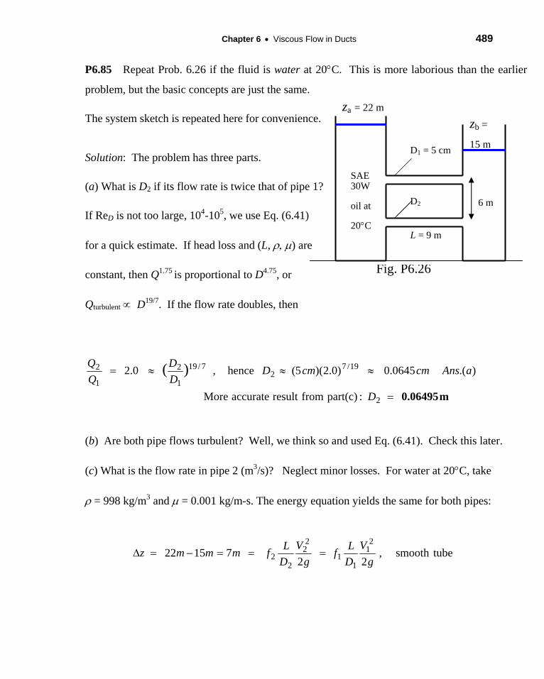
Chapter 6 • Viscous Flow in Ducts 489
P6.85 Repeat Prob. 6.26 if the fluid is water at 20°C. This is more laborious than the earlier
problem, but the basic concepts are just the same.
The system sketch is repeated here for convenience. za = 22 m
zb =
15 m D1 = 5 cm
Solution: The problem has three parts. SAE 30W
oil at
20°C
(a) What is D2 if its flow rate is twice that of pipe 1? D2 6 m
If ReD is not too large, 104-105, we use Eq. (6.41)
L = 9 m for a quick estimate. If head loss and (L, ρ, μ) are
Fig. P6.26 constant, then Q1.75 is proportional to D4.75, or
Qturbulent ∝ D19/7. If the flow rate doubles, then
m0.06495=
≈≈≈=
2
19/72
7/19
1
2
1
2
:part(c)fromresultaccurateMore
).(0645.0)0.2)(5(hence,0.2 )(
D
aAnscmcmDDD
(b) Are both pipe flows turbulent? Well, we think so and used Eq. (6.41). Check this later.
(c) What is the flow rate in pipe 2 (m3/s)? Neglect minor losses. For water at 20°C, take
ρ = 998 kg/m3 and μ = 0.001 kg/m-s. The energy equation yields the same for both pipes:
tubesmooth,22
715222
1
11
22
22 g
VDLf
gV
DLfmmmz ===−=Δ

490 Solutions Manual • Fluid Mechanics, Fifth Edition
Since we don’t know ReD, or even know the exact D2, this requires either iteration or
EES. The results (obtained by EES) are:
13
2222
1111
2/02908.0;;01285.0;000,569Re
;05.0)(;01391.0;000,370Re
QsmQDf
QmgivenDf
=====
====
m0.06495
/sm0.01454 3
The Reynolds numbers are too high for the power-law, Eq. (6.41), but the error is only
0.7%.
6.86 SAE 10 oil at 20°C flows at an average velocity of 2 m/s between two smooth parallel horizontal plates 3 cm apart. Estimate (a) the centerline velocity, (b) the head loss per meter, and (c) the pressure drop per meter.
Solution: For SAE 10 oil, take ρ = 870 kg/m3 and μ = 0.104 kg/m⋅s. The half-distance between plates is called “h” (see Fig. 6.37). Check Dh and Re:
hh
h D4A VD 870(2.0)(0.06)D 4h 6 cm, Re 1004 (laminar)P 0.104
ρμ
= = = = = ≈
CL max3 3Then u u V (2.0) / (a)2 2
Ans.= = = ≈ 3.0 m s
The head loss and pressure drop per meter folow from laminar theory, Eq. (6.63):
2 23 VL 3(0.104)(2.0)(1.0)p /
h (0.015 m) (c)Ans.μ
Δ = = ≈ 2770 Pa m
fp 2770h /g 870(9.81)
Ans.ρΔ
= = ≈ 0.325 m m (b)
6.87 A commercial-steel annulus 40 ft long, with a = 1 in and b = 12 in, connects two
reservoirs which differ in surface height by 20 ft. Compute the flow rate in ft3/s through the annulus if the fluid is water at 20°C.
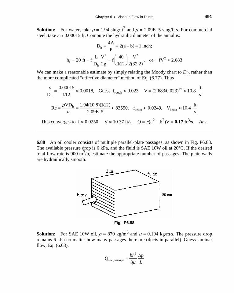
Chapter 6 • Viscous Flow in Ducts 491
Solution: For water, take ρ = 1.94 slug/ft3 and μ = 2.09E−5 slug/ft⋅s. For commercial steel, take ε ≈ 0.00015 ft. Compute the hydraulic diameter of the annulus:
h4AD 2(a b) 1 inch;= = − =
2 22
fh
PL V 40 Vh 20 ft f f , or: fV 2.683
D 2g 1/12 2(32.2)⎛ ⎞
= = = ≈⎜ ⎟⎝ ⎠
We can make a reasonable estimate by simply relating the Moody chart to Dh, rather than the more complicated “effective diameter” method of Eq. (6.77). Thus
1/2rough
h
0.00015 ft0.0018, Guess f 0.023, V (2.683/0.023) 10.8 D 1/12ε
= ≈ ≈ = ≈s
hbetter better
VD 1.94(10.8)(1/12) ftRe 83550, f 0.0249, V 10.4 2.09E 5 s
ρμ
= = ≈ ≈ ≈−
This converges to f ≈ 0.0250, V ≈ 10.37 ft/s, Q = π(a2 − b2)V = 0.17 ft3/s. Ans.
6.88 An oil cooler consists of multiple parallel-plate passages, as shown in Fig. P6.88. The available pressure drop is 6 kPa, and the fluid is SAE 10W oil at 20°C. If the desired total flow rate is 900 m3/h, estimate the appropriate number of passages. The plate walls are hydraulically smooth.
Fig. P6.88
Solution: For SAE 10W oil, ρ = 870 kg/m3 and μ = 0.104 kg/m⋅s. The pressure drop remains 6 kPa no matter how many passages there are (ducts in parallel). Guess laminar flow, Eq. (6.63),
3
3one passagebh pQ
LμΔ
=

492 Solutions Manual • Fluid Mechanics, Fifth Edition
where h is the half-thickness between plates. If there are N passages, then b = 50 cm for all and h = 0.5 m/(2N). We find h and N such that NQ = 900 m3/h for the full set of passages. The problem is ideal for EES, but one can iterate with a calculator also. We find that 18 passages are one too many—Q only equals 835 m3/h. The better solution is:
h3
D, 935 m /h, 1.47 cm, Re 512 (laminar flow)NQ h= = =N = 17 passages
6.89 An annulus of narrow clearance causes a very large pressure drop and is useful as an accurate measurement of viscosity. If a smooth annulus 1 m long with a = 50 mm and b = 49 mm carries an oil flow at 0.001 m3/s, what is the oil viscosity if the pressure drop is 250 kPa?
Solution: Assuming laminar flow, use Eq. (6.73) for the pressure drop and flow rate:
πμ
⎡ ⎤Δ −= − −⎢ ⎥
⎣ ⎦
4 4p (a b )Q a b , or, for the given data:8 L ln(a/b)
2 2 2
2 2 23 4 4250000 {(0.05) (0.049) }0.001 m /s (0.05) (0.049)
8 1 m ln(0.05/0.049)πμ
⎡ ⎤−⎛ ⎞= − −⎢ ⎥⎜ ⎟⎝ ⎠ ⎣ ⎦
Solve for / Ans.μ ≈ 0.0065 kg m s⋅
6.90 A 90-ft-long sheet-steel duct carries air at approximately 20°C and 1 atm. The duct cross section is an equilateral triangle whose side measures 9 in. If a blower can supply 1 hp to the flow, what flow rate, in ft3/s, will result?
Fig. P6.90
Solution: For air at 20°C and 1 atm, take ρ ≈ 0.00234 slug/ft3 and μ = 3.76E−7 slug/ft⋅s. Compute the hydraulic diameter, and express the head loss in terms of Q:
h4A 4(1/2)(9)(9sin 60 )D 5.2 0.433 ftP 3(9)
°= = = =′′
2 2 22
fh
L (Q/A) 90 {Q/[0.5(9/12) sin 60 ]}h f f 54.4fQD 2g 0.433 2(32.2)
°⎛ ⎞= = ≈⎜ ⎟⎝ ⎠

Chapter 6 • Viscous Flow in Ducts 493
For sheet steel, take ε ≈ 0.00015 ft, hence ε/Dh ≈ 0.000346. Now relate everything to the input power:
2f
ft lbfPower 1 hp 550 gQh (0.00234)(32.2)Q[54.4fQ ],s
ρ
3 3
31/3 h
or: fQ 134 with Q in ft /s
ft (Q/A)DGuess f 0.02, Q (134/0.02) 18.9 , Re 209000s
ρμ
⋅= = = =
≈
≈ = ≈ = ≈
Iterate: fbetter ≈ 0.0179, Qbetter ≈ 19.6 ft3/s, Rebetter ≈ 216500. The process converges to
f ≈ 0.01784, V ≈ 80.4 ft/s, Q ≈ 19.6 ft3/s. Ans.
6.91 Heat exchangers often consist of many triangular passages. Typical is Fig. P6.91, with L = 60 cm and an isosceles-triangle cross section of side length a = 2 cm and included angle β = 80°. If the average velocity is V = 2 m/s and the fluid is SAE 10 oil at 20°C, estimate the pressure drop.
Fig. P6.91
Solution: For SAE 10 oil, take ρ = 870 kg/m3 and μ = 0.104 kg/m⋅s. The Reynolds number based on side length a is Re = ρVa/μ ≈ 335, so the flow is laminar. The bottom side of the triangle is 2(2 cm)sin40° ≈ 2.57 cm. Calculate hydraulic diameter:
2h
1 4(2.57)(2cos40 ) 1.97 cm ; P 6.57 cm; D 1.20 cm2 P
A = ° ≈ = = ≈A
hh
DVD 870(2.0)(0.0120)Re 201; from Table 6.4, 40 , fRe 52.9
0.104ρ θ
μ= = ≈ = ° ≈
2 252.9 L 0.6 870Then f 0.263, p f V (0.263) (2)ρ ⎛ ⎞ ⎛ ⎞= ≈ Δ = =h201 D 2 0.012 2
Ans.
⎜ ⎟ ⎜ ⎟⎝ ⎠ ⎝ ⎠
≈ 23000 Pa

494 Solutions Manual • Fluid Mechanics, Fifth Edition
6.92 A large room uses a fan to draw in atmospheric air at 20°C through a 30 cm by 30 cm commercial-steel duct 12 m long, as in Fig. P6.92. Estimate (a) the air flow rate in m3/hr if the room pressure is 10 Pa vacuum; and (b) the room pressure if the flow rate is 1200 m3/hr. Neglect minor losses.
Fig. P6.92
Solution: For air, take ρ = 1.2 kg/m3 and μ = 1.8E−5 kg/m⋅s. For commercial steel, ε = 0.046 mm. For a square duct, Dh = side-length = 30 cm, hence ε/d = 0.046/300 = 0.000153. The (b) part is easier, with flow rate known we can evaluate velocity, Reynolds number, and friction factor:
1200/3600 1.2(3.70)(0.3)3.70 , 74100, thus 0.0198(0.3)(0.3) 1.8 5hD Moody
Q mV fA s E
= = = = = ≈−
Re
Then the pressure drop follows immediately:
2 212 1.20.0198 (3.70) 6.53 ,L2 0.3 2
or: ( ) (b)h
p f V Paρ ⎛ ⎞ ⎛ ⎞Δ = = =D
vacuum Ans.
⎜ ⎟ ⎜ ⎟⎝ ⎠ ⎝ ⎠
roomp 6.5 Pa=
(a) If Δp = 10 Pa (vacuum) is known, we must iterate to find friction factor:
22
12 1.2 1.2 (0.3)10 , , , 0.0001530.3 2 1.8 5(0.3) h
Q Vp Pa f V V f fcnE D
ε⎛ ⎞⎛ ⎞ ⎛ ⎞Δ = = = = =⎜ ⎟ ⎜ ⎟ ⎜ ⎟⎝ ⎠ ⎝ ⎠ −⎝ ⎠
After iteration, the results converge to:
V = 4.69 m/s; Red = 93800; f = 0.0190; Q = 0.422 m3/s = 1520 m3/h Ans. (a)
P6.93 In Moody’s Example 6.6, the 6-inch diameter, 200-ft-long asphalted cast iron pipe has a pressure drop of about 280 lbf/ft2 when the average water velocity is 6 ft/s. Compare this to an annular cast iron pipe with an inner diameter of 6 in and the same annular average velocity of 6 ft/s. (a) What outer diameter would cause the flow to have the same pressure drop of 280 lbf/ft2? (b) How do the cross-section areas compare, and why? Use the hydraulic diameter approximation.
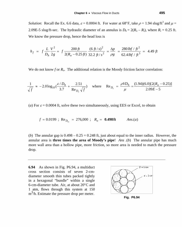
Chapter 6 • Viscous Flow in Ducts 495
Solution: Recall the Ex. 6.6 data, ε = 0.0004 ft. For water at 68°F, take ρ = 1.94 slug/ft3 and μ =
2.09E-5 slug/ft-sec. The hydraulic diameter of an annulus is Dh = 2(Ro – Ri), where Ri = 0.25 ft.
We know the pressure drop, hence the head loss is
ftftlbfftlbf
gp
sftsft
ftRftf
gV
DLfh
ohf 49.4
/4.62/280
/2.32)/6(
)25.0(2200
2 3
2
2
22==
Δ=
−==
ρ
We do not know f or Ro. The additional relation is the Moody friction factor correlation:
509.2)]25.0(2)[0.6)(94.1(
Rewhere)Re
51.27.3
/(log0.21
10 −−
==+−≈E
RVDf
Df
ohD
D
hh
hμ
ρε
(a) For ε = 0.0004 ft, solve these two simultaneously, using EES or Excel, to obtain
).(;000,276Re;0199.0 aAnsRf oDhoft0.498===
(b) The annular gap is 0.498 – 0.25 = 0.248 ft, just about equal to the inner radius. However, the annular area is three times the area of Moody’s pipe! Ans .(b) The annular pipe has much more wall area than a hollow pipe, more friction, so more area is needed to match the pressure drop.
6.94 As shown in Fig. P6.94, a multiduct cross section consists of seven 2-cm-diameter smooth thin tubes packed tightly in a hexagonal “bundle” within a single 6-cm-diameter tube. Air, at about 20°C and 1 atm, flows through this system at 150 m3/h. Estimate the pressure drop per meter.
Fig. P6.94

496 Solutions Manual • Fluid Mechanics, Fifth Edition
Solution: For air, take ρ = 1.2 kg/m3 and μ = 1.8E−5 kg/m⋅s. A separate analysis would show that the small triangular cusped passages have fifty times more resistance to the flow than the 2-cm-diameter tubes. Therefore we assume all the flow goes through the seven 2-cm tubes. Thus each tube takes one-seventh of the flow rate:
27 tubes
Q 150/3600 m Vd 1.2(18.95)(0.02)V 18.95 , Re 25300A s 1.8E 57 (0.01)
ρμπ
= = ≈ = = ≈−
2 2L 1.0 1.2ρ ⎛ ⎞smoothTurbulent: f 0.0245, p f V 0.0245 (18.95)
d 2 0.02 2p Ans.
≈ Δ = = ⎜ ⎟⎝ ⎠
Δ ≈ 260 Pa
6.95 A wind tunnel is made of wood and is 28 m long, with a rectangular section 50 cm by 80 cm. It draws in sea-level standard air with a fan. If the fan delivers 7 kW of power to the air, estimate (a) the average velocity; and (b) the pressure drop in the wind tunnel.
Solution: For sea-level air, ρ = 1.22 kg/m3 and μ = 1.81E−5 kg/m⋅s. The hydraulic diameter is:
4 4(50 )(80 ) 61.54 0.6154 2(50 80 )h
A cm cmD cP cm
= = = =+
m m
(a, b) The known power is related to both the flow rate and the pressure drop:
2[ ]2h
LPower Q p HWV f VD
ρ⎡ ⎤= Δ = ⎢ ⎥
⎣ ⎦
3W=
ns.
2 328 1.22 /[(0.5 )(0.8 ) ] 11.1 7000 0.6154 2
m kg mm m V f V fVm
⎡ ⎤= =⎢ ⎥
⎣ ⎦
Thus we need to find V such that fV3 = 631 m3/s3. For wood, take roughness ε = 0.5 mm. Then ε/Dh = 0.0005 m/0.6154 m = 0.000813. Use the Moody chart to find V and the Reynolds number. Guess f ≈ 0.02 to start, or use EES. The iteration converges to:
0.0189, Re 1.33E6, / (a, b)hDf A= = ΔV p= =32 m s, 540 Pa
6.96 Water at 20°C is flowing through a 20-cm-square smooth duct at a (turbulent) Reynolds number of 100,000. For a “laminar
flow element” measurement, it is desired to pack the pipe with a honeycomb array of small square passages (see Fig. P6.28 for

Chapter 6 • Viscous Flow in Ducts 497
an example). What passage width h will ensure that the flow in each tube will be laminar (Reynolds number less than 2000)?
Fig. P6.96
Solution: The hydraulic diameter of a square is the side length h (or a). For water, take ρ = 998 kg/m3 and μ = 0.001 kg/m⋅s. The Reynolds number establishes flow velocity:
998 (0.2)100,000 ,0.001hD
Vd VRe ρμ
= = = Solve for 0.501 mVs
=
This velocity is the same when we introduce small passages, if we neglect the blockage of the thin passage walls. Thus we merely set the passage Reynolds number = 2000:
998(0.501) 2000 0.001h
Vh hRe if hρμ
= ≤ ≤ 0.004 m 4 mm= Ans.
6.97 A heat exchanger consists of multiple parallel-plate passages, as shown in Fig. P6.97. The available pressure drop is 2 kPa, and the fluid is water at 20°C. If the desired total flow rate is 900 m3/h, estimate the appropriate number of passages. The plate walls are hydraulically smooth.
Fig. P6.97
Solution: For water, ρ = 998 kg/m3 and μ = 0.001 kg/m⋅s. Unlike Prob. 6.88, here we expect turbulent flow. If there are N passages, then b = 50 cm for all N and the passage thickness is H = 0.5 m/N. The hydraulic diameter is Dh = 2H. The velocity in each passage is related to the pressure drop by Eq. (6.58):
2 where2
hsmooth
h
VDLp f V f f fcnD
ρρμ
⎛ ⎞Δ = = = ⎜ ⎟⎝ ⎠
322.0 998 /For the given data, 2000
2(0.5 / ) 2m kg mPa f V
m N=

498 Solutions Manual • Fluid Mechanics, Fifth Edition
Select N, find H and V and Qtotal = AV = b2V and compare to the desired flow of 900 m3/h. For example, guess N = 20, calculate f = 0.0173 and Qtotal = 2165 m3/h. The converged result is
3
ns.total 908 m /h, 0.028,
Re 14400, 7.14 mm,hD
Q f
H A
= =
= = N = 70 passages
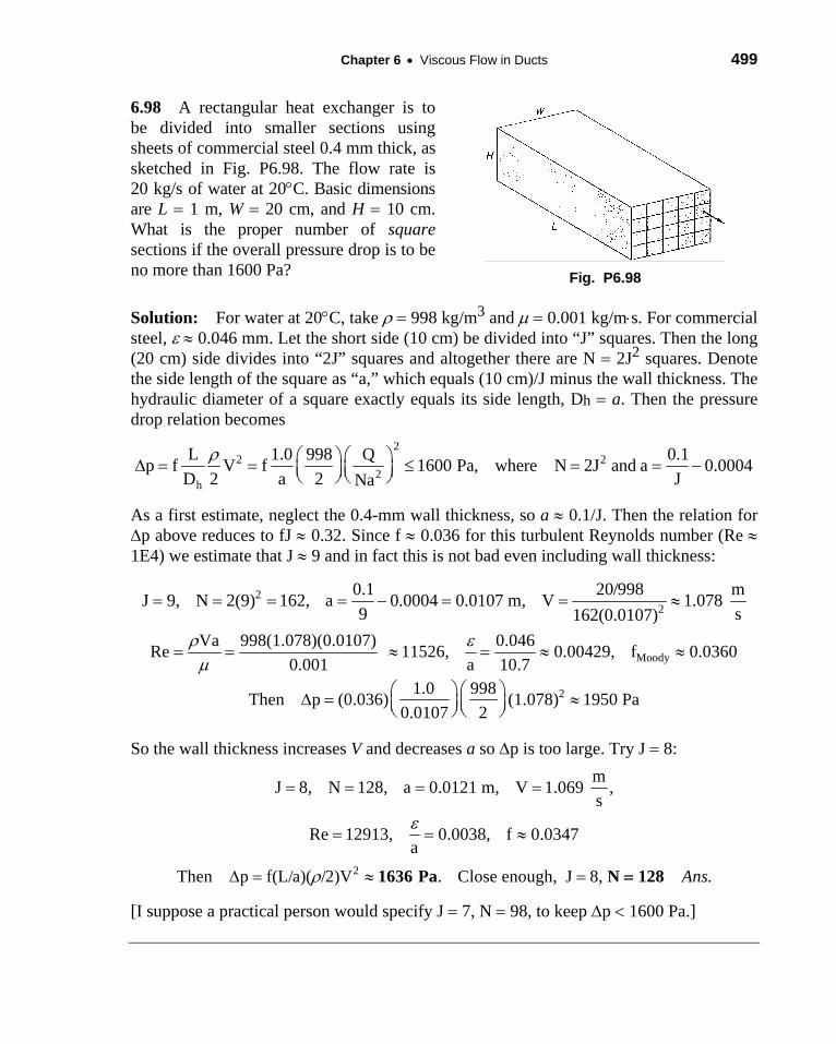
Chapter 6 • Viscous Flow in Ducts 499
6.98 A rectangular heat exchanger is to be divided into smaller sections using sheets of commercial steel 0.4 mm thick, as sketched in Fig. P6.98. The flow rate is 20 kg/s of water at 20°C. Basic dimensions are L = 1 m, W = 20 cm, and H = 10 cm. What is the proper number of square sections if the overall pressure drop is to be no more than 1600 Pa?
Fig. P6.98
Solution: For water at 20°C, take ρ = 998 kg/m3 and μ = 0.001 kg/m⋅s. For commercial steel, ε ≈ 0.046 mm. Let the short side (10 cm) be divided into “J” squares. Then the long (20 cm) side divides into “2J” squares and altogether there are N = 2J2 squares. Denote the side length of the square as “a,” which equals (10 cm)/J minus the wall thickness. The hydraulic diameter of a square exactly equals its side length, Dh = a. Then the pressure drop relation becomes
21600 Pa, where N 2J22
h
L 1.0 998 Q 0.1p f V f and a 0.0004D 2 a 2 JNa
ρ ⎛ ⎞ ⎛ ⎞Δ = = ≤ = = −⎜ ⎟ ⎜ ⎟⎝ ⎠ ⎝ ⎠
2
As a first estimate, neglect the 0.4-mm wall thickness, so a ≈ 0.1/J. Then the relation for Δp above reduces to fJ ≈ 0.32. Since f ≈ 0.036 for this turbulent Reynolds number (Re ≈ 1E4) we estimate that J ≈ 9 and in fact this is not bad even including wall thickness:
22
0.1 20/998 mJ 9, N 2(9) 162, a 0.0004 0.0107 m, V 1.078 9 s162(0.0107)
= = = = − = = ≈
MoodyVa 998(1.078)(0.0107) 0.046Re 11526, 0.00429, f 0.0360
0.001 a 10.7ρ ε
μ= = ≈ = ≈ ≈
21.0 998Then p (0.036) (1.078) 1950 Pa0.0107 2
⎛ ⎞ ⎛ ⎞Δ = ≈⎜ ⎟ ⎜ ⎟⎝ ⎠ ⎝ ⎠
So the wall thickness increases V and decreases a so Δp is too large. Try J = 8: mJ 8, N 128, a 0.0121 m, V 1.069 ,= = = =s
Re 12913, 0.0038, f 0.0347aε
= = ≈
2Then p f(L/a)( /2)V . Close enough, J 8, Ans.ρΔ = ≈ =1636 Pa N 128=
[I suppose a practical person would specify J = 7, N = 98, to keep Δp < 1600 Pa.]
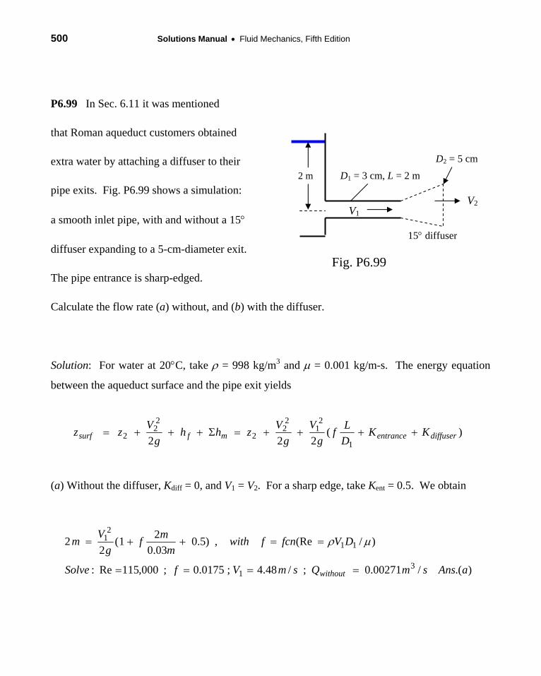
500 Solutions Manual • Fluid Mechanics, Fifth Edition
P6.99 In Sec. 6.11 it was mentioned
that Roman aqueduct customers obtained
extra water by attaching a diffuser to their
pipe exits. Fig. P6.99 shows a simulation:
a smooth inlet pipe, with and without a 15°
diffuser expanding to a 5-cm-diameter exit.
The pipe entrance is sharp-edged.
Calculate the flow rate (a) without, and (b) with the diffuser.
Solution: For water at 20°C, take ρ = 998 kg/m3 and μ = 0.001 kg/m-s. The energy equation
between the aqueduct surface and the pipe exit yields
(a) Without the diffuser, Kdiff = 0, and V1 = V2. For a sharp edge, take Kent = 0.5. We obtain
D1 = 3 cm, L = 2 m D2 = 5 cm
2 m
V2V1
15° diffuser
Fig. P6.99
)(222 1
21
22
2
22
2 diffuserentrancemfsurf KKDLf
gV
gVzhh
gVzz ++++=Σ+++=
).(/00271.0;/48.4;0175.0;000,115Re:
)/(Re,)5.003.021(
22
31
11
21
aAnssmQsmVfSolve
DVfcnfwithm
mfg
Vm
without ====
==++= μρ
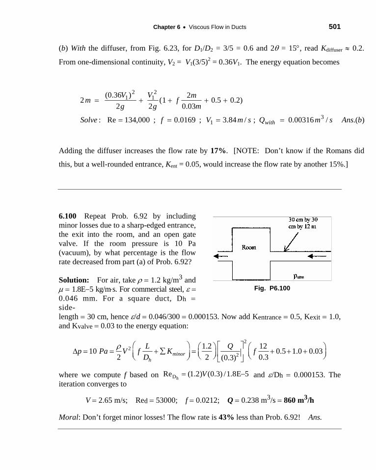
Chapter 6 • Viscous Flow in Ducts 501
(b) With the diffuser, from Fig. 6.23, for D1/D2 = 3/5 = 0.6 and 2θ = 15°, read Kdiffuser ≈ 0.2.
From one-dimensional continuity, V2 = V1(3/5)2 = 0.36V1. The energy equation becomes
).(/00316.0;/84.3;0169.0;000,134Re:
)2.05.003.021(
22)36.0(2
31
21
21
bAnssmQsmVfSolve
mmf
gV
gVm
with ====
++++=
Adding the diffuser increases the flow rate by 17%. [NOTE: Don’t know if the Romans did
this, but a well-rounded entrance, Kent = 0.05, would increase the flow rate by another 15%.]
6.100 Repeat Prob. 6.92 by including minor losses due to a sharp-edged entrance, the exit into the room, and an open gate valve. If the room pressure is 10 Pa (vacuum), by what percentage is the flow rate decreased from part (a) of Prob. 6.92?
Solution: For air, take ρ = 1.2 kg/m3 and μ = 1.8E−5 kg/m⋅s. For commercial steel, ε = 0.046 mm. For a square duct, Dh = side-
Fig. P6.100
length = 30 cm, hence ε/d = 0.046/300 = 0.000153. Now add Kentrance = 0.5, Kexit = 1.0, and Kvalve = 0.03 to the energy equation:
2⎞⎟⎠
e (1.2) (0.3) /1.8E 5V
22
1.2 1210 0.5 1.0 0.032 2 0.3(0.3)h
L Qp Pa V f K fD
ρ ⎛ ⎞ ⎡ ⎤⎛ ⎞ ⎛Δ = = + ∑ = + + +⎜ ⎟ ⎜⎢ ⎥⎜ ⎟ ⎝ ⎠ ⎝⎝ ⎠ ⎣ ⎦minor
where we compute f based on RhD = − and ε/Dh = 0.000153. The
iteration converges to
V = 2.65 m/s; Red = 53000; f = 0.0212; Q = 0.238 m3/s = 860 m3/h
Moral: Don’t forget minor losses! The flow rate is 43% less than Prob. 6.92! Ans.
502 Solutions Manual • Fluid Mechanics, Fifth Edition

Chapter 6 • Viscous Flow in Ducts 503
NOTE: IN PROBLEMS 6.100−6.110, MINOR LOSSES ARE INCLUDED.
6.101 In Fig. P6.101 a thick filter is being tested for losses. The flow rate in the pipe is 7 m3/min, and the upstream pressure is 120 kPa. The fluid is air at 20°C. Using the water-manometer reading, estimate the loss coefficient K of the filter.
Fig. P6.101
Solution: The upstream density is ρair = p/(RT) = 120000/[287(293)] = 1.43 kg/m3. The average velocity V (which is used to correlate loss coefficient) follows from the flow rate:
3s2
7/60 / 14.85 /( /4)(0.1 )pipe
Q m sV mA mπ
= = =
The manometer measures the pressure drop across the filter: 3 2( ) (998 1.43 / )(9.81 / )(0.04 ) 391 mano w a manop gh kg m m s m Paρ ρΔ = − = − =
This pressure is correlated as a loss coefficient using Eq. (6.78):
2 3 2391
(1/2) (1/2)(1.43 / )(14.85 / )filter
filterp PaK A
V kg m m sρ
Δ= = ≈ 2.5 ns.
6.102 A 70 percent efficient pump deli-vers water at 20°C from one reservoir to another 20 ft higher, as in Fig. P6.102. The piping system consists of 60 ft of galvanized-iron 2-in pipe, a reentrant entrance, two screwed 90° long-radius elbows, a screwed-open gate valve, and a sharp exit. What is the input power required in horsepower with and without a 6° well-designed conical expansion added to the exit? The flow rate is 0.4 ft3/s.
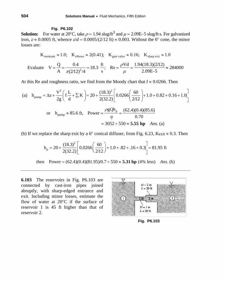
504 Solutions Manual • Fluid Mechanics, Fifth Edition
Fig. P6.102 Solution: For water at 20°C, take ρ = 1.94 slug/ft3 and μ = 2.09E−5 slug/ft⋅s. For galvanized iron, ε ≈ 0.0005 ft, whence ε/d = 0.0005/(2/12 ft) ≈ 0.003. Without the 6° cone, the minor losses are:
reentrant elbows gate valve sharp exitK 1.0; K 2(0.41); K 0.16; K 1.0≈ ≈ ≈ ≈
2Q 0.4 ft Vd 1.94(18.3)(2/12)Evaluate V 18.3 ; Re 284000A s 2.09E 5(2/12) /4
ρμπ
= = = = = ≈−
At this Re and roughness ratio, we find from the Moody chart that f ≈ 0.0266. Then
2 2
pumpV L (18.3) 60(a) h z f K 20 0.0266 1.0 0.82 0.16 1.02g d 2(32.2) 2/12
⎡ ⎤⎛ ⎞⎛ ⎞= Δ + + ∑ = + + + + +⎢ ⎥⎜ ⎟ ⎜ ⎟⎝ ⎠ ⎝ ⎠⎣ ⎦
pgQh (62.4)(0.4)(85.6)pumpor h 85.6 ft, Power
0.703052 550 (a)Ans.
ρη
≈ = =
= ÷ ≈ 5.55 hp
(b) If we replace the sharp exit by a 6° conical diffuser, from Fig. 6.23, Kexit ≈ 0.3. Then
2
p(18.3) 60h 20 0.0266 1.0 .82 .16 0.3 81.95 ft2(32.2) 2/12
⎡ ⎤⎛ ⎞= + + + + + =⎢ ⎥⎜ ⎟⎝ ⎠⎣ ⎦
then Power (62.4)(0.4)(81.95)/0.7 550 (4% less) (b)Ans.= ÷ ≈ 5.31 hp
6.103 The reservoirs in Fig. P6.103 are connected by cast-iron pipes joined abruptly, with sharp-edged entrance and exit. Including minor losses, estimate the flow of water at 20°C if the surface of reservoir 1 is 45 ft higher than that of reservoir 2.
Fig. P6.103

Chapter 6 • Viscous Flow in Ducts 505
Solution: For water at 20°C, take ρ = 1.94 slug/ft3 and μ = 2.09E−5 slug/ft⋅s. Let “a” be the small pipe and “b” the larger. For wrought iron, ε ≈ 0.00015 ft, whence ε/da = 0.0018 and ε/db = 0.0009. From the continuity relation,
2 2a a b b b a b
1Q V d V d or, since d 2d , we obtain V V4 4 4π π
= = = = a
For pipe “a” there are two minor losses: a sharp entrance, K1 = 0.5, and a sudden expansion, Fig. 6.22, Eq. (6.101), K2 = [1 − (1/2)2]2 ≈ 0.56. For pipe “b” there is one minor loss, the submerged exit, K3 ≈ 1.0. The energy equation, with equal pressures at (1) and (2) and near zero velocities at (1) and (2), yields
2 2 ⎞⎟⎠
a a b bf-a m-a f-b m-b a b
a b
V L V Lz h h h h f 0.5 0.56 f 1.0 ,2g d 2g d
⎛ ⎞ ⎛Δ = + ∑ + + ∑ = + + + +⎜ ⎟ ⎜⎝ ⎠ ⎝
2a
b a a bV 120 1.0or, since V V /4, z 45 ft 240f 1.06 f
2(32.2) 16 16⎡ ⎤= Δ = = + + +⎢ ⎥⎣ ⎦
where fa and fb are separately related to different values of Re and ε/d. Guess to start:
a b a a a a-2f f 0.02: then V 21.85 ft/s, Re 169000, /d 0.0018, f 0.0239ε≈ ≈ = ≈ = ≈
b b b b-2V 5.46 ft/s, Re 84500, /d 0.0009, f 0.0222ε= ≈ = ≈
a b a
a a
Converges to: f 0.024, f 0.0224, V 20.3 ft/s,
Q V A . Ans.
= = ≈
= ≈ 30.111 ft /s
6.104 Reconsider the air hockey table of Problem 3.162, but with inclusion of minor losses. The table is 3 ft by 6 ft in area, with 1/16-in-diameter holes spaced every inch in a rectangular grid (2592 holes total). The required jet speed from each hole is 50 ft/s. Your job is to select an appropriate blower to meet the requirements.
Fig. P3.162
Hint: Assume that the air is stagnant in the manifold under the table surface, and assume sharp-edge inlets at each hole. (a) Estimate the pressure rise (in lbf/in2) required of the blower. (b) Compare your answer to the previous calculation in Prob. 3.162, where minor losses were ignored. Are minor losses significant?
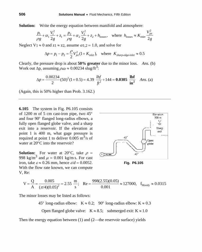
506 Solutions Manual • Fluid Mechanics, Fifth Edition
Solution: Write the energy equation between manifold and atmosphere: 22 2
21 1 2 2
1 1 2 2 , where2 2
jetlosses losses inlet
Vp V p Vz z h h Kg g g g
α αρ ρ
+ + = + + + ≈g
Neglect V1 ≈ 0 and z1 ≈ z2, assume α1,2 = 1.0, and solve for 2
1 2 - -(1 ), where 0.52 jet inlet sharp edge inletp p p V K Kρ
Δ = − = + ≈
Clearly, the pressure drop is about 50% greater due to the minor loss. Ans. (b) Work out Δp, assuming ρair ≈ 0.00234 slug/ft3:
22
0.00234 (50) (1 0.5) 4.39 144 (a)2
lbfp Aft
Δ = + = ÷ = 2lbf0.0305in
ns.
(Again, this is 50% higher than Prob. 3.162.)
6.105 The system in Fig. P6.105 consists of 1200 m of 5 cm cast-iron pipe, two 45° and four 90° flanged long-radius elbows, a fully open flanged globe valve, and a sharp exit into a reservoir. If the elevation at point 1 is 400 m, what gage pressure is required at point 1 to deliver 0.005 m3/s of water at 20°C into the reservoir?
Solution: For water at 20°C, take ρ = 998 kg/m3 and μ = 0.001 kg/m⋅s. For cast iron, take ε ≈ 0.26 mm, hence ε/d = 0.0052. With the flow rate known, we can compute V, Re:
Fig. P6.105
Moody2Q 0.005 m 998(2.55)(0.05)V 2.55 ; Re 127000, f 0.0315A s 0.001( /4)(0.05)π
= = = = ≈ ≈
The minor losses may be listed as follows:
45 long-radius elbow: K 0.2; 90 long-radius elbow: K 0.3° ≈ ° ≈
Open flanged globe valve: K 8.5; submerged exit: K 1.0≈ ≈
Then the energy equation between (1) and (2—the reservoir surface) yields

Chapter 6 • Viscous Flow in Ducts 507
2
m,1 11 2 f
p V z 0 0 z h hg 2gρ
+ + = + + + + ∑
2
1(2.55) 1200or: p /( g) 500 400 0.0315 0.5 2(0.2) 4(0.3) 8.5 1 12(9.81) 0.05
ρ ⎡ ⎤⎛ ⎞= − + + + + + + −⎜ ⎟⎢ ⎥⎝ ⎠⎣ ⎦
100 253 353 m, or: (998)(9.81)(353) Ans.= + = = ≈1p 3.46 MPa
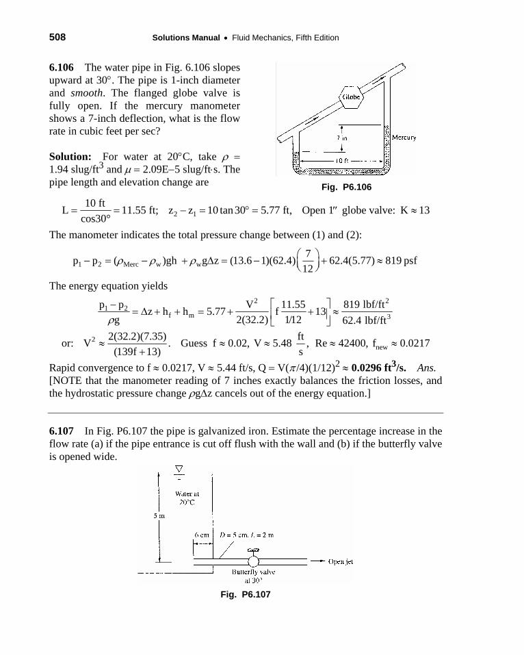
508 Solutions Manual • Fluid Mechanics, Fifth Edition
6.106 The water pipe in Fig. 6.106 slopes upward at 30°. The pipe is 1-inch diameter and smooth. The flanged globe valve is fully open. If the mercury manometer shows a 7-inch deflection, what is the flow rate in cubic feet per sec?
Solution: For water at 20°C, take ρ = 1.94 slug/ft3 and μ = 2.09E−5 slug/ft⋅s. The pipe length and elevation change are
Fig. P6.106
2 110 ftL 11.55 ft; z z 10 tan30 5.77 ft, Open 1 globe valve: K 13
cos30°= = − = ° = ≈′′
The manometer indicates the total pressure change between (1) and (2):
1 2 Merc w w7p p ( )gh g z (13.6 1)(62.4) 62.4(5.77) 819 psf
12ρ ρ ρ ⎛ ⎞− = − + Δ = − + ≈⎜ ⎟⎝ ⎠
The energy equation yields 2 2
1 2f m 3
p p V 11.55 819 lbf/ftz h h 5.77 f 13g 2(32.2) 1/12 62.4 lbf/ftρ
⎡ ⎤−= Δ + + = + + ≈⎢ ⎥
⎣ ⎦
2new
2(32.2)(7.35) ftor: V . Guess f 0.02, V 5.48 , Re 42400, f 0.0217(139f 13) s
≈ ≈ ≈ ≈+
≈
Rapid convergence to f ≈ 0.0217, V ≈ 5.44 ft/s, Q = V(π /4)(1/12)2 ≈ 0.0296 ft3/s. Ans. [NOTE that the manometer reading of 7 inches exactly balances the friction losses, and the hydrostatic pressure change ρgΔz cancels out of the energy equation.]
6.107 In Fig. P6.107 the pipe is galvanized iron. Estimate the percentage increase in the flow rate (a) if the pipe entrance is cut off flush with the wall and (b) if the butterfly valve is opened wide.
Fig. P6.107

Chapter 6 • Viscous Flow in Ducts 509
Solution: For water at 20°C, take ρ = 998 kg/m3 and μ = 0.001 kg/m⋅s. For galvanized iron, take ε ≈ 0.15 mm, hence ε/d = 0.003. First establish minor losses as shown:
Protruding entrance (Fig. 6.21a), L 1.2, K 1;d
≈ ≈
Butterfly @ 30° (Fig 6.19) K ≈ 80 ± 20
The energy equation, with p1 = p2, yields:
2 2 2 mf m
V V L V 2z h h 1 f K 1 f 1.0 80 20 52g 2g d 2(9.81) 0.05
⎡ ⎤⎡ ⎤ ⎛ ⎞Δ = + + ∑ = + + ∑ = + + + ± =⎜ ⎟⎢ ⎥⎢ ⎥ ⎝ ⎠⎣ ⎦ ⎣ ⎦
new new
smf 0.0284, V 1.086 s
dmGuess f 0.02, V 1.09 , Re 54300, 0.003,ε
≈ ≈ ≈ =
≈ ≈
Thus the “base” flow, for our comparison, is Vo ≈ 1.086 m/s, Qo ≈ 0.00213 m3/s. If we cut off the entrance flush, we reduce Kent from 1.0 to 0.5; hardly a significant reduction in view of the huge butterfly valve loss Kvalve ≈ 80. The energy equation is
Q
2(9.81) s
(0.3% more) (a)Ans.3m0.00214
s=
2V m5 m [1 40f 0.5 80 20], solve V 1.090 ,= + + + ± ≈
If we open the butterfly wide, Kvalve decreases from 80 to only 0.3, a huge reduction:
Q
2(9.81) s
(5 times more) (b)Ans.=3m0.0106
s
2V m5 m [1 40f 1.0 0.3], solve V 5.4 ,= + + + ≈
Obviously opening the valve has a dominant effect for this system.
6.108 The water pump in Fig. P6.108 maintains a pressure of 6.5 psig at point 1. There is a filter, a half-open disk valve, and two regular screwed elbows. There are 80 ft of 4-inch diameter commercial steel pipe. (a) If the flow rate is 0.4 ft3/s, what is the loss coefficient of the filter? (b) If the disk valve is wide open and Kfilter = 7, what is the resulting flow rate?
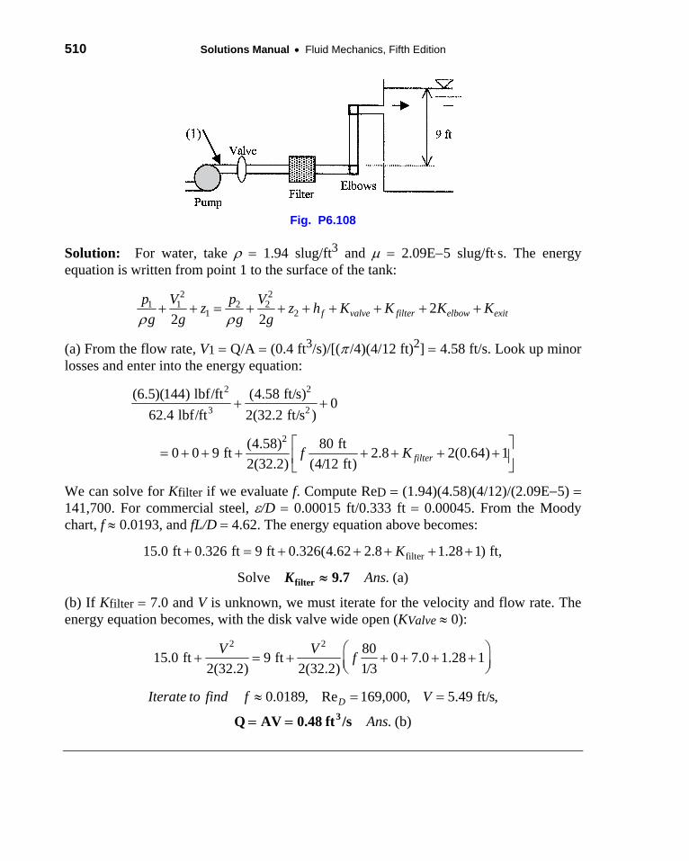
510 Solutions Manual • Fluid Mechanics, Fifth Edition
Fig. P6.108
Solution: For water, take ρ = 1.94 slug/ft3 and μ = 2.09E−5 slug/ft⋅s. The energy equation is written from point 1 to the surface of the tank:
2 21 1 2 2
1 2 22 2 f valve filter elbow exit
p V p Vz z h K K Kg g g gρ ρ
+ + = + + + + + + + K
(a) From the flow rate, V1 = Q/A = (0.4 ft3/s)/[(π /4)(4/12 ft)2] = 4.58 ft/s. Look up minor losses and enter into the energy equation:
+ +2 2
3 2(6.5)(144) lbf/ft (4.58 ft/s) 0
+ = + + + + +
⎡ ⎤= + + + + + + +⎢ ⎥
⎣ ⎦
2
62.4 lbf/ft 2(32.2 ft/s )
(4.58) 80 ft0 0 9 ft 2.8 2(0.64) 12(32.2) (4/12 ft) filterf K
We can solve for Kfilter if we evaluate f. Compute ReD = (1.94)(4.58)(4/12)/(2.09E−5) = 141,700. For commercial steel, ε/D = 0.00015 ft/0.333 ft = 0.00045. From the Moody chart, f ≈ 0.0193, and fL/D = 4.62. The energy equation above becomes:
filter15.0 ft 0.326 ft 9 ft 0.326(4.62 2.8 1.28 1) ft,
Solve (a)
K
Ans.Kfilter 9.7≈
(b) If Kfilter = 7.0 and V is unknown, we must iterate for the velocity and flow rate. The energy equation becomes, with the disk valve wide open (KValve ≈ 0):
⎛ ⎞+ = + + + +⎜ ⎟⎝ ⎠
8015.0 ft 9 ft 0 7.0 1.28 12(32.2) 2(32.2) 1/3
V V f +2 2
≈ = =0.0189, Re 169,000, 5.49 ft/s,
(b)DIterate to find f V
Ans.3Q AV 0.48 ft /s= =
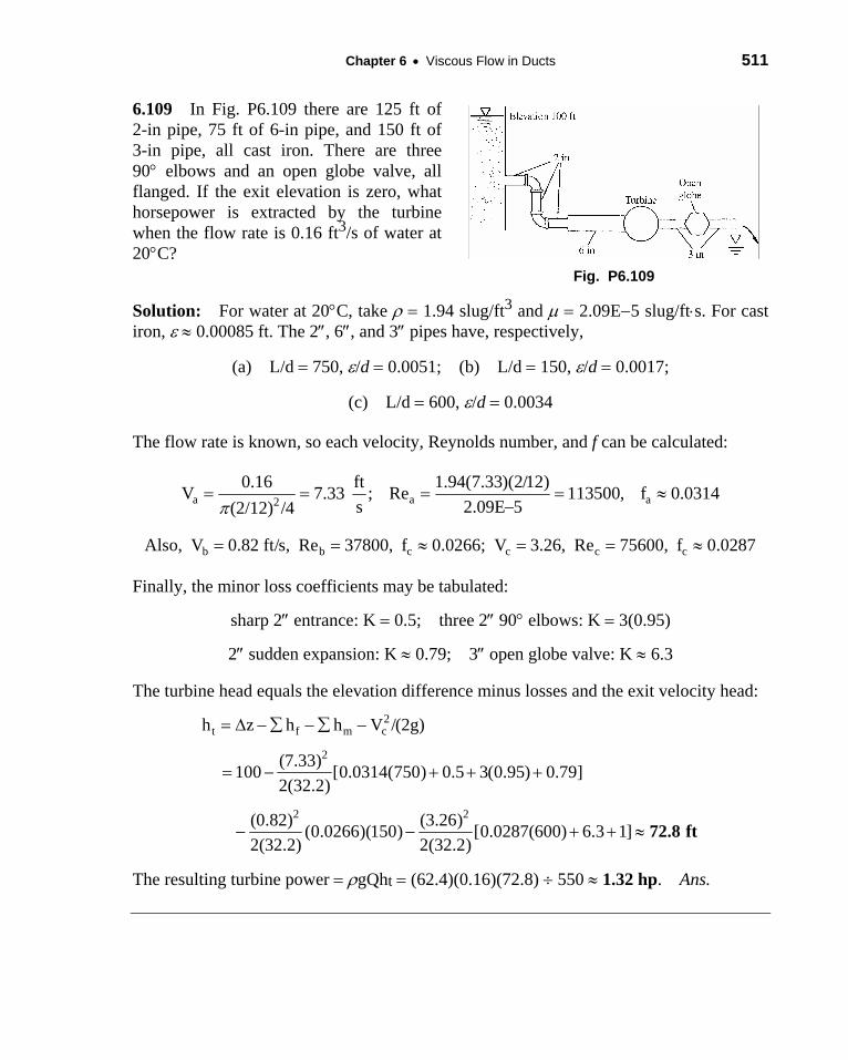
Chapter 6 • Viscous Flow in Ducts 511
6.109 In Fig. P6.109 there are 125 ft of 2-in pipe, 75 ft of 6-in pipe, and 150 ft of 3-in pipe, all cast iron. There are three 90° elbows and an open globe valve, all flanged. If the exit elevation is zero, what horsepower is extracted by the turbine when the flow rate is 0.16 ft3/s of water at 20°C?
Fig. P6.109
Solution: For water at 20°C, take ρ = 1.94 slug/ft3 and μ = 2.09E−5 slug/ft⋅s. For cast iron, ε ≈ 0.00085 ft. The 2″, 6″, and 3″ pipes have, respectively,
(a) L/d = 750, ε/d = 0.0051; (b) L/d = 150, ε/d = 0.0017;
(c) L/d = 600, ε/d = 0.0034
The flow rate is known, so each velocity, Reynolds number, and f can be calculated:
a a20.16 ft 1.94(7.33)(2/12)V 7.33 ; Re 113500, f 0.0314
s 2.09E 5(2/12) /4π= = = = ≈
− a
b b c c c cAlso, V 0.82 ft/s, Re 37800, f 0.0266; V 3.26, Re 75600, f 0.0287= = ≈ = = ≈
Finally, the minor loss coefficients may be tabulated:
sharp 2″ entrance: K = 0.5; three 2″ 90° elbows: K = 3(0.95)
2″ sudden expansion: K ≈ 0.79; 3″ open globe valve: K ≈ 6.3
The turbine head equals the elevation difference minus losses and the exit velocity head: 2
t f m c
2
h z h h V /(2g)= Δ − ∑ − ∑ −
≈2 2
(7.33)100 [0.0314(750) 0.5 3(0.95) 0.79]2(32.2)
(0.82) (3.26)(0.0266)(150) [0.0287(600) 6.3 1] 2(32.2) 2(32.2)
= − + + +
− − + + 72.8 ft
The resulting turbine power = ρgQht = (62.4)(0.16)(72.8) ÷ 550 ≈ 1.32 hp. Ans.

512 Solutions Manual • Fluid Mechanics, Fifth Edition
6.110 In Fig. P6.110 the pipe entrance is sharp-edged. If the flow rate is 0.004 m3/s, what power, in W, is extracted by the turbine?
Solution: For water at 20°C, take ρ = 998 kg/m3 and μ = 0.001 kg/m⋅s. For cast
Fig. P6.110
iron, ε ≈ 0.26 mm, hence ε/d = 0.26/50 ≈ 0.0052. The minor loss coefficients are Entrance: K ≈ 0.5; 5-cm(≈2″) open globe valve: K ≈ 6.9.
The flow rate is known, hence we can compute V, Re, and f:
2Q 0.004 m 998(2.04)(0.05)V 2.04 , Re 102000, f 0.0316A s 0.001( /4)(0.05)π
= = = = ≈ ≈
The turbine head equals the elevation difference minus losses and exit velocity head:
⎡ ⎤⎛ ⎞= Δ − − ∑ − = − + + + ≈⎜ ⎟⎢ ⎥⎝ ⎠⎣ ⎦t f m
V (2.04) 125h z h h 40 (0.0316) 0.5 6.9 1 21.5 m2g 2(9.81) 0.05
2 2
tPower gQh (998)(9.81)(0.004)(21.5) Ans.ρ= = ≈ 840 W
6.111 For the parallel-pipe system of Fig. P6.111, each pipe is cast iron, and the pressure drop p1 − p2 = 3 lbf/in2. Compute the total flow rate between 1 and 2 if the fluid is SAE 10 oil at 20°C.
Fig. P6.111
Solution: For SAE 10 oil at 20°C, take ρ = 1.69 slug/ft3 and μ = 0.00217 slug/ft⋅s. For cast iron, ε ≈ 0.00085 ft. Convert Δp = 3 psi = 432 psf and guess laminar flow in each:
3ft0.0763 Check Re (OK)
a
a
d (3/12)
.Q 300 s
π π
≈ ≈
a a aa 4 4
? 128 L Q 128(0.00217)(250)Qp 432 ,μΔ = = =
3ft0.0188 Re
b b bb 4 4
? 128 L Q 128(0.00217)(200)Qp 432 ,μΔ = = =
b
b
d (2/12)
Q . Check 112 (OK)s
π π
≈ ≈
a bThe total flow rate is Q Q 0.0763 0.0188 / . Ans.= + = + ≈ 3Q 0.095 ft s
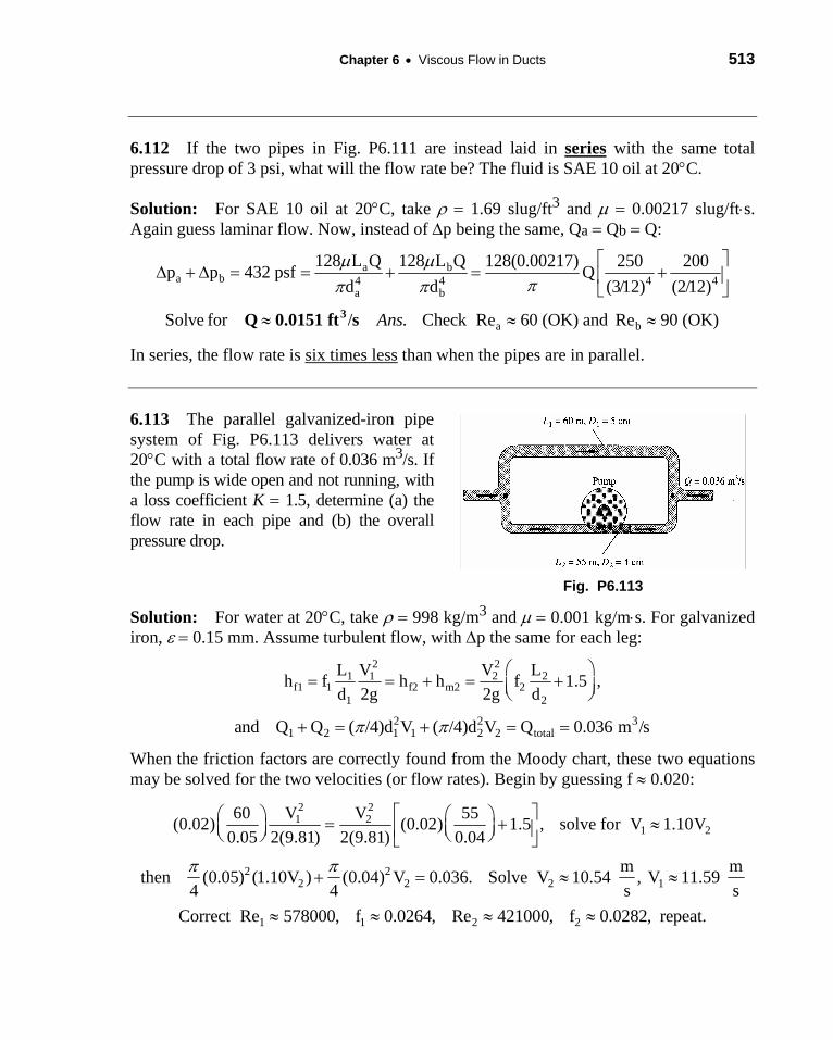
Chapter 6 • Viscous Flow in Ducts 513
6.112 If the two pipes in Fig. P6.111 are instead laid in series with the same total pressure drop of 3 psi, what will the flow rate be? The fluid is SAE 10 oil at 20°C.
Solution: For SAE 10 oil at 20°C, take ρ = 1.69 slug/ft3 and μ = 0.00217 slug/ft⋅s. Again guess laminar flow. Now, instead of Δp being the same, Qa = Qb = Q:
4 4250 200
(312) (212)a b
a b 4 4a b
128 L Q 128 L Q 128(0.00217)p p 432 psf Qd d / /
μ μππ π
⎡ ⎤Δ + Δ = = + = +⎢ ⎥
⎣ ⎦
Solve for a b / Check Re 60 (OK) and Re 90 (OK)Ans.≈ ≈3Q 0.0151 ft s ≈
In series, the flow rate is six times less than when the pipes are in parallel.
6.113 The parallel galvanized-iron pipe system of Fig. P6.113 delivers water at 20°C with a total flow rate of 0.036 m3/s. If the pump is wide open and not running, with a loss coefficient K = 1.5, determine (a) the flow rate in each pipe and (b) the overall pressure drop.
Fig. P6.113
Solution: For water at 20°C, take ρ = 998 kg/m3 and μ = 0.001 kg/m⋅s. For galvanized iron, ε = 0.15 mm. Assume turbulent flow, with Δp the same for each leg:
2 2,
3
1 1 2 2f1 1 f2 m2 2
1 2
L V V Lh f h h f 1.5d 2g 2g d
⎛ ⎞= = + = +⎜ ⎟⎝ ⎠
2 21 2 1 1 2 2 totaland Q Q ( /4)d V ( /4)d V Q 0.036 m /sπ π+ = + = =
When the friction factors are correctly found from the Moody chart, these two equations may be solved for the two velocities (or flow rates). Begin by guessing f ≈ 0.020:
2 2≈1 2
1 260 V V 55(0.02) (0.02) 1.5 , solve for V 1.10V
0.05 2(9.81) 2(9.81) 0.04⎡ ⎤⎛ ⎞ ⎛ ⎞= +⎜ ⎟ ⎜ ⎟⎢ ⎥⎝ ⎠ ⎝ ⎠⎣ ⎦
2 22 2 2 1
m mthen (0.05) (1.10V ) (0.04) V 0.036. Solve V 10.54 , V 11.59 4 4 sπ π
+ = ≈ ≈s
1 1 2 2Correct Re 578000, f 0.0264, Re 421000, f 0.0282, repeat.≈ ≈ ≈ ≈

514 Solutions Manual • Fluid Mechanics, Fifth Edition
The 2nd iteration converges: f1 ≈ 0.0264, V1 = 11.69 m/s, f2 ≈ 0.0282, V2 = 10.37 m/s,
Q1 = A1V1 = 0.023 m3/s, Q2 = A2V2 = 0.013 m3/s. Ans. (a)
The pressure drop is the same in either leg: 2 2
1 1 2 21 2
1 2
L V L Vp f f 1.5 (b)d 2 d 2
Ans.ρ ρ⎛ ⎞Δ = = + ≈⎜ ⎟⎝ ⎠
2.16E6 Pa
*P6.114 A blower supplies standard air to a plenum that feeds two horizontal square sheet-metal ducts with sharp-edged entrances. One duct is 100 ft long, with a cross-section 6 in by 6 in. The second duct is 200 ft long. Each duct exhausts to the atmosphere. When the plenum pressure is 5.0 lbf/ft2 gage, the volume flow in the longer duct is three times the flow in the shorter duct. Estimate both volume flows and the cross-section size of the longer duct.
Solution: For standard air, in BG units, take ρ = 0.00238 slug/ft3 and μ = 3.78E-7 slug/ft-
sec. For sheet-metal, take ε = 0.00016 ft. The energy equation for this case is
5.0)1(21
:,22
2
2
222
1
211
≈++=Δ
++++=++
−edgedsharpenth
entrancef
KwhereKDLfVp
orhhzg
Vg
pzg
Vg
p
ρ
ρρ
We have abbreviated the duct velocity to V, without a subscript. For a square duct, the
hydraulic diameter is the side length of the square. First compute the flow rate in the short
duct:
),(Re,)5.05.0
1001{2
/00238.00.53
2hhD D
fcnfftftfftslug
ftlbf ε
=++=
The Reynolds number for the short duct is Re = (0.00238)V(0.5)/(3.78E-7) = 3148V,
and ε/Dh = 0.00016ft/0.5ft = 0.00032. The solution is
/sft6.92 3===== shortD QsftVfftL ;/7.27;0200.0;000,87Re:100 h

Chapter 6 • Viscous Flow in Ducts 515
For the longer duct, Re = (0.00238)VDh /(3.78E-7), and ε/Dh = 0.00016ft/Dh. We don’t
know Dh and must solve to make Qlong = 3Qshort. The solution is
.forSolve
/75.20;/5.27;0177.0;000,150Re:200
,
3
AnsD
sftQsftVfftL
longh
longhD
ft0.87=
=====
NOTE: It is an interesting numerical quirk that, for these duct parameters, the velocities
in each duct are almost identical, regardless of the magnitude of the pressure drop.
6.115 In Fig. P6.115 all pipes are 8-cm-diameter cast iron. Determine the flow rate from reservoir (1) if valve C is (a) closed; and (b) open, with Kvalve = 0.5.
Fig. P6.115
Solution: For water at 20°C, take ρ = 998 kg/m3 and μ = 0.001 kg/m⋅s. For cast iron, ε ≈ 0.26 mm, hence ε/d = 0.26/80 ≈ 0.00325 for all three pipes. Note p1 = p2, V1 = V2 ≈ 0. These are long pipes, but we might wish to account for minor losses anyway:
sharp entrance at A: K1 ≈ 0.5; line junction from A to B: K2 ≈ 0.9 (Table 6.5)
branch junction from A to C: K3 ≈ 1.3; two submerged exits: KB = KC ≈ 1.0
If valve C is closed, we have a straight series path through A and B, with the same flow rate Q, velocity V, and friction factor f in each. The energy equation yields
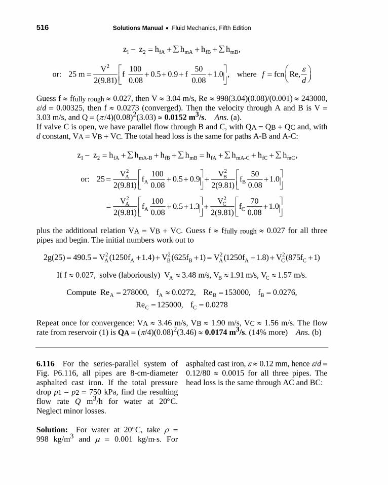
516 Solutions Manual • Fluid Mechanics, Fifth Edition
1 2 fA mA fB mBz z h h h h− = + ∑ + + ∑ ,
2V 100 50or: 25 m f 0.5 0.9 f 1.0 , where fcn Re,2(9.81) 0.08 0.08
fdε⎡ ⎤ ⎛= + + + + = ⎜ ⎟⎢ ⎥ ⎝ ⎠⎣ ⎦
⎞
Guess f ≈ ffully rough ≈ 0.027, then V ≈ 3.04 m/s, Re ≈ 998(3.04)(0.08)/(0.001) ≈ 243000, ε/d = 0.00325, then f ≈ 0.0273 (converged). Then the velocity through A and B is V = 3.03 m/s, and Q = (π /4)(0.08)2(3.03) ≈ 0.0152 m3/s. Ans. (a). If valve C is open, we have parallel flow through B and C, with QA = QB + QC and, with d constant, VA = VB + VB
,
C. The total head loss is the same for paths A-B and A-C:
1 2 fA mA-B fB mB fA mA-C fC mCz z h h h h h h h h− = + ∑ + + ∑ = + ∑ + + ∑
2 2A B
A BV 100 V 50or: 25 f 0.5 0.9 f 1.0⎡ ⎤ ⎡ ⎤= + + + +⎢ ⎥ ⎢ ⎥⎦
⎤+ ⎥⎦
≈
22CA
A C
2(9.81) 0.08 2(9.81) 0.08
VV 100 70f 0.5 1.3 f 1.02(9.81) 0.08 2(9.81) 0.08
⎣ ⎦ ⎣
⎡ ⎤ ⎡= + + +⎢ ⎥ ⎢⎣ ⎦ ⎣
plus the additional relation VA = VB + VC. Guess f ≈ ffully rough ≈ 0.027 for all three pipes and begin. The initial numbers work out to
2 2 2 2A A B B A A C C2g(25) 490.5 V (1250f 1.4) V (625f 1) V (1250f 1.8) V (875f 1)= = + + + = + + +
A B CIf f 0.027, solve (laboriously) V 3.48 m/s, V 1.91 m/s, V 1.57 m/s.≈ ≈ ≈
A A B B
C C
Compute Re 278000, f 0.0272, Re 153000, f 0.0276,Re 125000, f 0.0278
= ≈ = == =
Repeat once for convergence: VA ≈ 3.46 m/s, VB ≈ 1.90 m/s, VC ≈ 1.56 m/s. The flow rate from reservoir (1) is QA = (π/4)(0.08)2(3.46) ≈ 0.0174 m3/s. (14% more) Ans. (b)
6.116 For the series-parallel system of Fig. P6.116, all pipes are 8-cm-diameter asphalted cast iron. If the total pressure drop p1 − p2 = 750 kPa, find the resulting flow rate Q m3/h for water at 20°C. Neglect minor losses.
Solution: For water at 20°C, take ρ = 998 kg/m3 and μ = 0.001 kg/m⋅s. For
asphalted cast iron, ε ≈ 0.12 mm, hence ε/d = 0.12/80 ≈ 0.0015 for all three pipes. The head loss is the same through AC and BC:
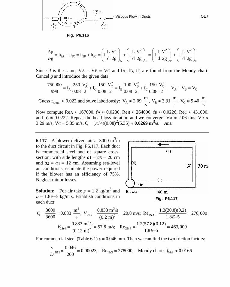
Chapter 6 • Viscous Flow in Ducts 517
Fig. P6.116
2 2 2 2
A C B C
V L V L V L Vf f fd 2g d 2g d 2g
⎛ ⎞ ⎛ ⎞ ⎛ ⎞ ⎛ ⎞+ = +⎜ ⎟ ⎜ ⎟ ⎜ ⎟ ⎜ ⎟
⎝ ⎠ ⎝ ⎠ ⎝ ⎠ ⎝ ⎠fA fC fB fC
p Lh h h h fg d 2gρ
Δ= + = + =
Since d is the same, VA + VB = VC and fA, fB, fC are found from the Moody chart. Cancel g and introduce the given data:
2 22 2
CV=C CA BA C B C A B
V V750000 250 V 150 100 V 150f f f f , V V998 0.08 2 0.08 2 0.08 2 0.08 2
= + = + +
rough A B Cm mGuess f 0.022 and solve laboriously: V 2.09 , V 3.31 , V 5.40 s s
≈ ≈ ≈ms
≈
Now compute ReA ≈ 167000, fA ≈ 0.0230, ReB ≈ 264000, fB ≈ 0.0226, ReC ≈ 431000, and fC ≈ 0.0222. Repeat the head loss iteration and we converge: VA ≈ 2.06 m/s, VB ≈ 3.29 m/s, VC ≈ 5.35 m/s, Q = (π / 4)(0.08)2(5.35) ≈ 0.0269 m3/s. Ans.
6.117 A blower delivers air at 3000 m3/h to the duct circuit in Fig. P6.117. Each duct is commercial steel and of square cross-section, with side lengths a1 = a3 = 20 cm and a2 = a4 = 12 cm. Assuming sea-level air conditions, estimate the power required if the blower has an efficiency of 75%. Neglect minor losses.
Solution: For air take ρ = 1.2 kg/m3 and μ = 1.8E−5 kg/m⋅s. Establish conditions in each duct:
Fig. P6.117
= = = = = =−1&3 1&32
3000 m 0.833 m /s 1.2(20.8)(0.2)0.833 ; 20.8 m/s; Re 278,0003600 s 1.8 5(0.2 m)
Q VE
3 3
= = = =−2&4 2&42
0.833 m /s 1.2(57.8)(0.12)57.8 m/s; Re 463,0001.8 5(0.12 m)
VE
3
For commercial steel (Table 6.1) ε = 0.046 mm. Then we can find the two friction factors:
1&3 1&3 1&30.046 0.00023; Re 278000; Moody chart: 0.0166200
fDε
= = = ≈|
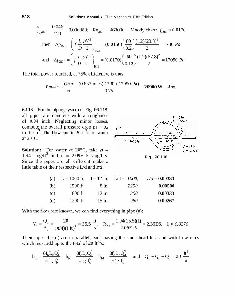
518 Solutions Manual • Fluid Mechanics, Fifth Edition
2&4 2&4 1&30.046 0.000383; Re 463000; Moody chart: 0.0170120
fDε
= = = ≈|
2 2Pa1&3
1&3
80 (1.2)(20.8)Then (0.0166) 1730 2 0.2 2
L Vp fD
ρ⎛ ⎞ ⎛ ⎞Δ = = =⎜ ⎟⎜ ⎟ ⎝ ⎠⎝ ⎠
2 2
Pa2&41&3
60 (1.2)(57.8)and (0.0170) 17050 2 0.12 2
L Vp fD
ρ⎛ ⎞ ⎛ ⎞Δ = = =⎜ ⎟⎜ ⎟ ⎝ ⎠⎝ ⎠
The total power required, at 75% efficiency, is thus:
ηΔ +
= = =(0.833 m /s)(1730 17050 Pa)
0.75Q pPower Ans.20900 W
3
6.118 For the piping system of Fig. P6.118, all pipes are concrete with a roughness of 0.04 inch. Neglecting minor losses, compute the overall pressure drop p1 − p2 in lbf/in2. The flow rate is 20 ft3/s of water at 20°C.
Solution: For water at 20°C, take ρ = 1.94 slug/ft3 and μ = 2.09E−5 slug/ft⋅s. Since the pipes are all different make a little table of their respective L/d and ε/d:
Fig. P6.118
(a) L = 1000 ft, d = 12 in, L/d = 1000, ε/d = 0.00333 (b) 1500 ft 8 in 2250 0.00500 (c) 800 ft 12 in 800 0.00333 (d) 1200 ft 15 in 960 0.00267
With the flow rate known, we can find everything in pipe (a):
aa a2
a
Q 20 ft 1.94(25.5)(1)V 25.5 , Re 2.36E6, fA s 2.09E 5( /4)(1 ft)π
= = = = = ≈−
0.0270a
Then pipes (b,c,d) are in parallel, each having the same head loss and with flow rates which must add up to the total of 20 ft3/s:
2 2 2 320 b b b c c c d d d
fb fc fd b c d2 5 2 5 2 5b c d
8f L Q 8f L Q 8f L Q fth h h , and Q Q Qsgd gd gdπ π π
= = = = = + + =

Chapter 6 • Viscous Flow in Ducts 519
Introduce Lb, db, etc. to find that Qc = 3.77Qb(fb/fc)1/2 and Qd = 5.38Qb(fb/fd)1/2
Then the flow rates are iterated from the relation 3
]
3
1/2 1/2b b c b d
ftQ 20 Q [1 3.77(f /f ) 5.38(f /f )s
∑ = = + +
3 3b c d b c dFirst guess: f f f : Q 1.97 ft /s; Q 7.43 ft /s; Q 10.6 ft /s= = ≈ ≈ ≈
Improve by computing Reb ≈ 349000, fb ≈ 0.0306, Rec ≈ 878000, fc ≈ 0.0271, Red ≈ 1002000, fd ≈ 0.0255. Repeat to find Qb ≈ 1.835 ft3/s, Qc ≈ 7.351 ft3/s, Qd ≈ 10.814 ft3/s. Repeat once more and quit: Qb ≈ 1.833 ft3/s, Qc ≈ 7.349 ft3/s, Qd ≈ 10.819 ft3/s, from which Vb ≈ 5.25 ft/s, Vc ≈ 9.36 ft/s, Vd ≈ 8.82 ft/s. The pressure drop is
2 2a a b bL V L V
p p p p f f1 2 a b a ba bd 2 d 2
17000 1800 18800 psf Ans.= + ≈ ≈ 2lbf131in
ρ ρ− = Δ + Δ = +
6.119 Modify Prob. 6.118 as follows. Let the pressure drop (p1 − p2) be 98 lbf/in2. Neglecting minor losses, determine the flow rate in ft3/s.
Solution: From the solution just above for Δp ≈ 131 psi, we can see that Δpa is about 90.2% of the total drop. Therefore our first guess can be that
2 2a a a
a aa
L V 1.94Vp 0.902 p 0.902(98 144) 12729 psf f (0.027)(1000)d 2 2
ρΔ ≈ Δ = × ≈ = ≈
a
31/2 1/2
a a a b b c b d?
sftand Q A V 17.3 Q [1 3.77(f /f ) 5.38(f /f ) ]s
= ≈ = + +
ftSolve for V 22.05 ≈
The last relation is still valid just as it was in Prob. 6.188. We can iterate to find 3 3 2
a b c d bft ft ftf 0.0270, Q 1.585 , Q 6.357 , Q 9.358 , f 0.0307s s s
≈ ≈ ≈ ≈ ≈
2 21 2 a a a a b b b bp p f (L /d )( V /2) f (L /d )( V /2) 12717 1382 14099 psf 97.9 psiρ ρ− = + ≈ + = ≈
This is certainly close enough. We conclude the flow rate is Q ≈ 17.3 ft3/s. Ans.
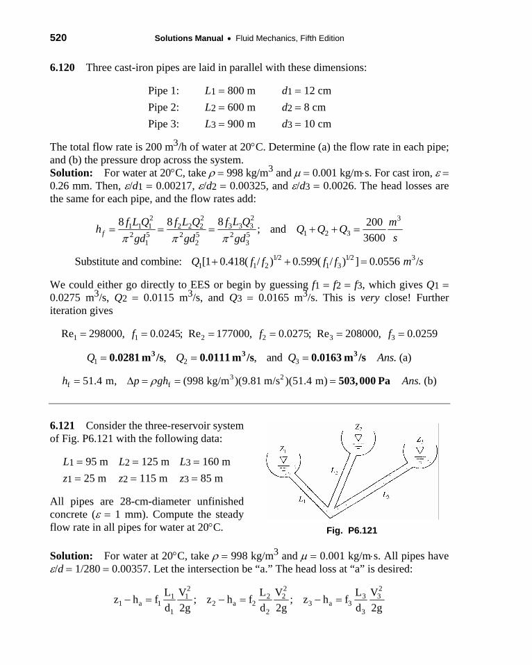
520 Solutions Manual • Fluid Mechanics, Fifth Edition
6.120 Three cast-iron pipes are laid in parallel with these dimensions:
Pipe 1: L1 = 800 m d1 = 12 cm Pipe 2: L2 = 600 m d2 = 8 cm Pipe 3: L3 = 900 m d3 = 10 cm
The total flow rate is 200 m3/h of water at 20°C. Determine (a) the flow rate in each pipe; and (b) the pressure drop across the system. Solution: For water at 20°C, take ρ = 998 kg/m3 and μ = 0.001 kg/m⋅s. For cast iron, ε = 0.26 mm. Then, ε/d1 = 0.00217, ε/d2 = 0.00325, and ε/d3 = 0.0026. The head losses are the same for each pipe, and the flow rates add:
22 2 3Q Q
m s
f
. (a)Ans
ns
3 3 31 1 1 2 2 21 2 32 5 2 5 2 5
1 2 3
88 8 200; and3600f
f L Qf L Q f L Q mh Qsgd gd gdπ π π
= = = + + =
1/2 1/2 31 1 2 1 3Substitute and combine: [1 0.418( / ) 0.599( / ) ] 0.0556 /Q f f f f+ + =
We could either go directly to EES or begin by guessing f1 = f2 = f3, which gives Q1 = 0.0275 m3/s, Q2 = 0.0115 m3/s, and Q3 = 0.0165 m3/s. This is very close! Further iteration gives
1 1 2 2 3 3Re 298000, 0.0245; Re 177000, 0.0275; Re 208000, 0.0259f f= = = = = =
1 2 3, , andQ Q Q= = =3 3 30.0281 m /s 0.0111 m /s 0.0163 m /s
3 2f f51.4 m, (998 kg/m )(9.81 m/s )(51.4 m) . (b)h p gh Aρ= Δ = = = 503, 000 Pa
6.121 Consider the three-reservoir system of Fig. P6.121 with the following data:
L1 = 95 m L2 = 125 m L3 = 160 mz1 = 25 m z2 = 115 m z3 = 85 m
All pipes are 28-cm-diameter unfinished concrete (ε = 1 mm). Compute the steady flow rate in all pipes for water at 20°C.
Fig. P6.121
Solution: For water at 20°C, take ρ = 998 kg/m3 and μ = 0.001 kg/m⋅s. All pipes have ε/d = 1/280 = 0.00357. Let the intersection be “a.” The head loss at “a” is desired:
22 2
3
3 31 1 2 21 a 1 2 a 2 3 a 3
1 2
L VL V L Vz h f ; z h f ; z h fd 2g d 2g d 2g
− = − = − =

Chapter 6 • Viscous Flow in Ducts 521
plus the requirement that Q1 + Q2 + Q3 = 0 or, for same d, V1 + V2 + V3 = 0
We guess ha then iterate each friction factor to find V and Q and then check if ∑Q = 0. 2
11
a 1 195 V mh 75 m: 25 75 ( )50 f , solve f 0.02754, V 10.25
0.28 2(9.81) s⎛ ⎞= − = − = ≈ ≈ −⎜ ⎟⎝ ⎠
22 2 2 2Similarly, 115 75 f (125/0.28) V /2(9.81) gives f 0.02755. V 7.99⎡ ⎤− = ≈ ≈ +⎣ ⎦
23 3
3 3
and 85 75 f (160/0.28) V /2(9.81)
mgives f 0.02762, V 3.53 , Vs
⎡ ⎤− = ⎣ ⎦
≈ ≈ + ∑ = +1.27
Repeating for ha = 80 m gives V1 = −10.75, V2 = +7.47, V3 = +2.49 m/s, ∑V = −0.79. Interpolate to ha ≈ 78 m, gives V1 = −10.55 m/s, V2 = +7.68 m/s, V3 = +2.95 m/s, or:
Q1 = −0.65 m3/s, Q2 = +0.47 m3/s, Q3 = +0.18 m3/s. Ans.
6.122 Modify Prob. 6.121 by reducing the diameter to 15 cm, with ε = 1 mm. Compute the flow rate in each pipe. They all reduce, compared to Prob. 6.121, by a factor of about 5.2. Can you explain this?
Solution: The roughness ratio increases to ε/d = 1/150 = 0.00667, and all L/d’s increase. Guess ha = 75 m: converges to f1 = 0.0333, f2 = 0.0333, f4 = 0.0334
and V1 ≈ −6.82 m/s, V2 ≈ +5.32 m/s, V3 ≈ +2.34 m/s, ∑V ≈ +0.85
We finally obtain ha ≈ 78.2 m, giving V1 = −7.04 m/s, V2 = +5.10 m/s, V3 = +1.94 m/s,
or: Q1 = −0.124 m3/s, Q2 = +0.090 m3/s, Q3 = +0.034 m3/s. Ans.
6.123 Modify Prob. 6.121 on the previous page as follows. Let z3 be unknown and find its value such that the flow rate in pipe 3 is 0.2 m3/s toward the junction. (This problem is best suited for computer iteration.)
Solution: For water at 20°C, take ρ = 998 kg/m3 and μ = 0.001 kg/m⋅s. All pipes have ε/d = 1/280 = 0.00357. Let the intersection be “a.” The head loss at “a” is desired for each in order to check the flow rate in pipe 3.
In Prob. 6.121, with z3 = 85 m, we found Q3 to be 0.18 m3/s toward the junction, pretty close. We repeat the procedure with a few new values of z3, closing to ∑Q = 0 each time:

522 Solutions Manual • Fluid Mechanics, Fifth Edition
33 a 1 2 3
3
Guess z 85 m: h 78.19 m, Q 0.6508, Q 0.4718, Q 0.1790 m /s
90 m: 80.65 m, 0.6657, 0.6657, 0.2099 m /s
= = = − = + = +
− + +
a 1
2
Interpolate: h 79.89, Q 0.6611,
Q 0.4608, , .Ans
≈ ≈ −
≈ + 33 3Q 0.200 m /s z 88.4 m≈ + ≈

Chapter 6 • Viscous Flow in Ducts 523
6.124 The three-reservoir system in Fig. P6.124 delivers water at 20°C. The system data are as follows:
D1 = 8 in D2 = 6 in D3 = 9 in
L1 = 1800 ft
L2 = 1200 ft L3 = 1600 ft
All pipes are galvanized iron. Compute the flow rate in all pipes.
Fig. P6.124
Solution: For water at 20°C, take ρ = 1.94 slug/ft3 and μ = 2.09E−5 slug/ft⋅s. For galvanized iron, take ε = 0.0005 ft. Then the roughness ratios are
1 2 3/ 0.00075 / 0.0010 / 0.00667d d dε ε ε= = =
Let the intersection be “a.” The head loss at “a” is desired:
22 23 3 31 1 1 2 2 2
1 a 2 a 3 a 1 2 31 2 3
f L Vf L V f L Vz h ; z h ; z h ; plus Q Q Q 0d 2g d 2g d 2g
− = − = − = + + =
We guess ha then iterate each friction factor to find V and Q and then check if ∑Q = 0. 2
1 1a
f (1800)VGuess h 50 ft: 20 50 ( )30 ft ,= − = − =
1 1
(8/12)2(32.2)ftsolve f 0.0194, V 6.09 s
= = −
32 2 3Similarly, f 0.0204, V 8.11 ft/s and of course V 0. Get Q 0.54 ft /s= ≈ + = ∑ = −
Try again with a slightly lower ha to reduce Q1 and increase Q2 and Q3:
3 3
a 1 2ft fth 48 ft: converges to Q 2.05 , Q 1.62 ,= = − = +
3
3
s sftQ 0.76 , Q 0.33s
= + ∑ = +
Interpolate to
ah 49.12 ft: / / / .Ans= 3 3 31 2 3Q 2.09 ft s, Q 1.61 ft s, Q 0.49 ft s= − = + = +
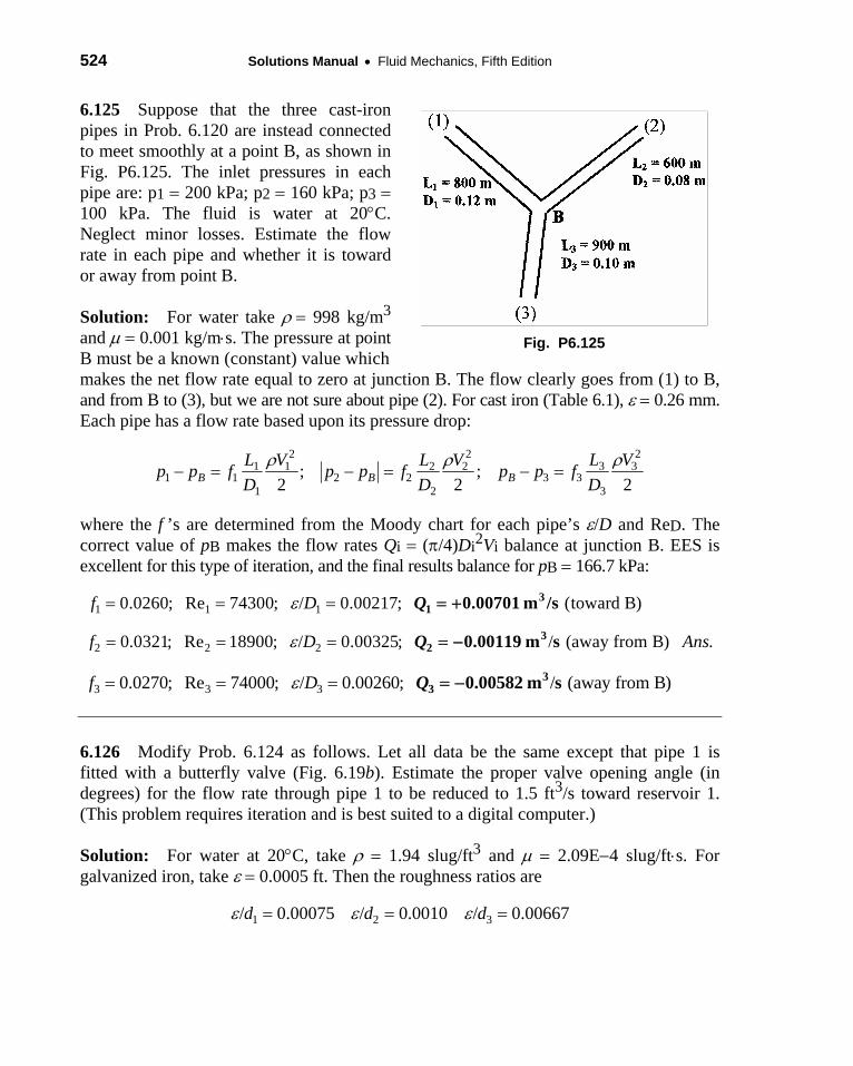
524 Solutions Manual • Fluid Mechanics, Fifth Edition
6.125 Suppose that the three cast-iron pipes in Prob. 6.120 are instead connected to meet smoothly at a point B, as shown in Fig. P6.125. The inlet pressures in each pipe are: p1 = 200 kPa; p2 = 160 kPa; p3 = 100 kPa. The fluid is water at 20°C. Neglect minor losses. Estimate the flow rate in each pipe and whether it is toward or away from point B.
Solution: For water take ρ = 998 kg/m3 and μ = 0.001 kg/m⋅s. The pressure at point B must be a known (constant) value which
Fig. P6.125
makes the net flow rate equal to zero at junction B. The flow clearly goes from (1) to B, and from B to (3), but we are not sure about pipe (2). For cast iron (Table 6.1), ε = 0.26 mm. Each pipe has a flow rate based upon its pressure drop:
22 2
3 23 31 1 2 2
1 1 2 2 3 31 2
; ;2 2B B B
L VL V L Vp p f p p f p p fD D D
ρρ ρ− = − = − =
where the f ’s are determined from the Moody chart for each pipe’s ε/D and ReD. The correct value of pB makes the flow rates Qi = (π/4)Di2Vi balance at junction B. EES is excellent for this type of iteration, and the final results balance for pB = 166.7 kPa: B
1 1 10.0260; Re 74300; / 0.00217; (toward B)f Dε= = = Q 31 0.00701 m /s= +
2 2 20.0321; Re 18900; / 0.00325; / (away from B) .f D Aε= = = Q 32 0.00119 m s= − ns
3 3 30.0270; Re 74000; / 0.00260; / (away from B)f Dε= = = Q 33 0.00582 m s= −
6.126 Modify Prob. 6.124 as follows. Let all data be the same except that pipe 1 is fitted with a butterfly valve (Fig. 6.19b). Estimate the proper valve opening angle (in degrees) for the flow rate through pipe 1 to be reduced to 1.5 ft3/s toward reservoir 1. (This problem requires iteration and is best suited to a digital computer.)
Solution: For water at 20°C, take ρ = 1.94 slug/ft3 and μ = 2.09E−4 slug/ft⋅s. For galvanized iron, take ε = 0.0005 ft. Then the roughness ratios are
1 2 3/ 0.00075 / 0.0010 / 0.00667d d dε ε ε= = =

Chapter 6 • Viscous Flow in Ducts 525
For a butterfly valve loss coefficient “K” (to be found). Let the junction be “J.” The head loss at “J” is desired and then to be iterated to give the proper flow rate in pipe (1):
2 21 2
1 J 2 JV L V Lz h f K ; z h f ;⎛ ⎞ ⎛ ⎞− = + − =⎜ ⎟ ⎜ ⎟⎠1 2
23
3 J 1 2 33
2g d 2g d
V Lz h f ; and Q Q Q 02g d
⎝ ⎠ ⎝
⎛ ⎞− = + + =⎜ ⎟⎝ ⎠
We know z1 = 20 ft, z2 = 100 ft, and z3 = 50 ft. From Prob. 6.124, where K = 0, the flow rate was 2.09 ft3/s toward reservoir 1. Now guess a finite value of K and repeat:
3 3J 1 2K 40: converges to h 50.0, Q 1.59 ft /s, Q 1.59 ft /s; Q 0= = = − = + 3 ≈
3
J 1 2 3K 50: converges to h 50.03 ft, Q 1.513 Q 1.591 Q 0.078= = = − = + = −
J 2: gives h 50.04 ft, / Q 1.591 Q 0.091 Ans.= =31K 52 Q 1.500 ft s= = − = −
From Fig. 6.19b, a butterfly valve coefficient K ≈ 52 occurs at θopening ≈ 35°. Ans.
6.127 In the five-pipe horizontal network of Fig. P6.127, assume that all pipes have a friction factor f = 0.025. For the given inlet and exit flow rate of 2 ft3/s of water at 20°C, determine the flow rate and direction in all pipes. If pA = 120 lbf/in2 gage, deter-mine the pressures at points B, C, and D.
Solution: For water at 20°C, take ρ = 1.94 slug/ft3 and μ = 2.09E−5 slug/ft⋅s. Each pipe has a head loss which is known except for the square of the flow rate:
Fig. P6.127
222AC
f AC AC AC AC2 5 2 58(0.025)(3000)Q8fLQPipe AC: h K Q , where K 60.42
gd (32.2)(6/12)π π= = = ≈|
3
AB BC CD BDftSimilarly, K 19.12, K 13.26, K 19.12, K 1933. Q in s
⎛ ⎞= = = = ⎜ ⎟⎝ ⎠
There are two triangular closed loops, and the total head loss must be zero for each. Using the flow directions assumed on the figure P6.127 above, we have
2 2 2AB BC ACLoop A-B-C: 19.12Q 13.26Q 60.42Q 0+ − =
2 2 2BC CD BDLoop B-C-D: 13.26Q 19.12Q 1933.0Q 0+ − =

526 Solutions Manual • Fluid Mechanics, Fifth Edition
And there are three independent junctions which have zero net flow rate:
AB AC AB BC BD AC BC CDJunction A: Q Q 2.0; B: Q Q Q ; C: Q Q Q+ = = + + =
These are five algebraic equations to be solved for the five flow rates. The answers are:
AB AC BC CD BD Q , Q , Q , Q , Q (a)Ans.= = = = =ft1.19 0.81 0.99 1.80 0.20s
3
The pressures follow by starting at A (120 psi) and subtracting off the friction losses: 2 2
B A AB ABp p gK Q 120 144 62.4(19.12)(1.19)ρ= − = × −
Bp 15590 psf 144 = ÷ = 2lbf108in
C DSimilarly, p and p (b)Ans.≈ ≈103 psi 76 psi
6.128 Modify Prob. 6.127 above as follows: Let the inlet flow at A and the exit flow at D be unknown. Let pA − pB = 100 psi. Compute the flow rate in all five pipes.
Solution: Our head loss coefficients “K” from above are all the same. Head loss AB is known, plus we have two “loop” equations and two “junction” equations:
2 2A BAB AB AB AB
p p 100 144 231 ft K Q 19.12Q , or Q /g 62.4ρ
− ×= = = = = 33.47 ft s
2 2BC ACTwo loops: 231 13.26Q 60.42Q 0+ − =
2 2 2BC CD BD13.26Q 19.12Q 1933.0Q 0+ − =
Two junctions: QAB = 3.47 = QBC + QBD; QAC + QBC = QCD
The solutions are in exactly the same ratio as the lower flow rates in Prob. 6.127:
AB BC BD Q , Q , Q ,= = =3 3 3ft ft ft3.47 2.90 0.58
s
CD ACQ , Q .Ans= =3 3
s sft ft5.28 2.38s s
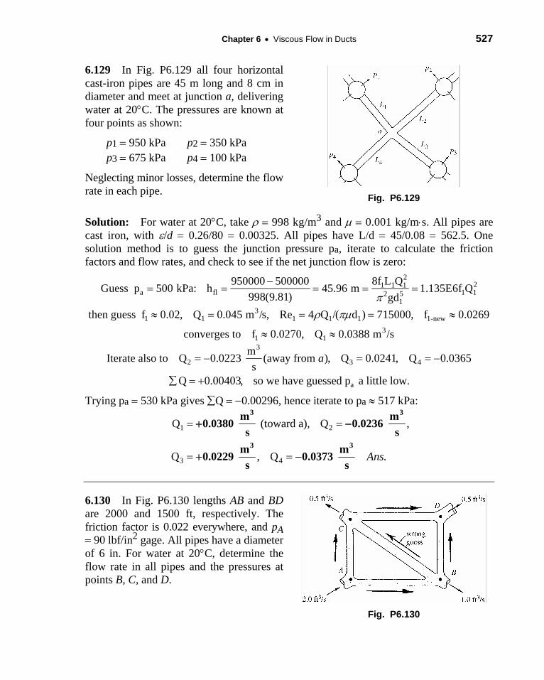
Chapter 6 • Viscous Flow in Ducts 527
6.129 In Fig. P6.129 all four horizontal cast-iron pipes are 45 m long and 8 cm in diameter and meet at junction a, delivering water at 20°C. The pressures are known at four points as shown:
p1 = 950 kPa p2 = 350 kPa p3 = 675 kPa p4 = 100 kPa
Neglecting minor losses, determine the flow rate in each pipe.
Fig. P6.129
Solution: For water at 20°C, take ρ = 998 kg/m3 and μ = 0.001 kg/m⋅s. All pipes are cast iron, with ε/d = 0.26/80 = 0.00325. All pipes have L/d = 45/0.08 = 562.5. One solution method is to guess the junction pressure pa, iterate to calculate the friction factors and flow rates, and check to see if the net junction flow is zero:
2
3
21 1 1a fl 1 12 5
1
950000 500000 8f L QGuess p 500 kPa: h 45.96 m 1.135E6f Q998(9.81) gdπ
−= = = = =
1 1 1 1 1 1-new3
1 1
then guess f 0.02, Q 0.045 m /s, Re 4 Q /( d ) 715000, f 0.0269
converges to f 0.0270, Q 0.0388 m /s
ρ πμ≈ = = = ≈
≈ ≈
3
42 3mIterate also to Q 0.0223 (away from ), Q 0.0241, Q 0.0365s
a= − = = −
aQ 0.00403, so we have guessed p a little low.∑ = +
Trying pa = 530 kPa gives ∑Q = −0.00296, hence iterate to pa ≈ 517 kPa:
1 2Q (toward a), Q ,= =+ −3 3m m0.0380 0.0236
3 4Q , Q Ans.= =+ −3 3
s sm m0.0229 0.0373s s
6.130 In Fig. P6.130 lengths AB and BD are 2000 and 1500 ft, respectively. The friction factor is 0.022 everywhere, and pA = 90 lbf/in2 gage. All pipes have a diameter of 6 in. For water at 20°C, determine the flow rate in all pipes and the pressures at points B, C, and D.
Fig. P6.130
528 Solutions Manual • Fluid Mechanics, Fifth Edition
Solution: For water at 20°C, take ρ = 1.94 slug/ft3 and μ = 2.09E−5 slug/ft⋅s. Each pipe has a head loss which is known except for the square of the flow rate:
22
AC2AC
f AC AC2 5 2 58(0.022)(1500)Q8fLQPipe AC: h K Q , where K
gd (32.2)(6/12)π π= = = ≈ 26.58
Similarly, KAB = KCD = 35.44, KBD = 26.58, and KBC = 44.30.
The solution is similar to Prob. 6.127, except that (1) the K’s are different; and (2) junctions B and C have additional flow leaving the network. The basic flow relations are:
2 2 2AB BC ACLoop ABC: 35.44Q 44.3Q 26.58Q 0+ − =
2 2 2BC CD BDLoop BCD: 44.3Q 35.44Q 26.58Q 0+ − =
AB AC
AB BC BD AC BC CD
Junctions A,B,C: Q Q 2.0;Q Q Q 1.0; Q Q Q 0.5
+ =
= + + + = +
In this era of PC “equation solvers” such as MathCAD, etc., it is probably not necessary to dwell upon any solution methods. For hand work, one might guess QAB, then the other four are obtained in sequence from the above relations, plus a check on the original guess for QAB. The assumed arrows are shown above. It turns out that we have guessed the direction incorrectly on QBC above, but the others are OK. The final results are:
AB ACQ / (toward B); Q / (toward C)= =3 30.949 ft s 1.051 ft s
BC CD BDQ (toward B); Q (toward D); Q (to D) (a)Ans.= = =0.239 0.312 0.188
The pressures start at A, from which we subtract the friction losses in each pipe: 2 2
B A AB ABp p gK Q 90 144 62.4(35.44)(0.949) 10969 psf 144ρ= − = × − = ÷ = 76 psi
C DSimilarly, we obtain p 11127 psf ; p 10911 psf . (b)Ans= = = ≈77 psi 76 psi
6.131 A water-tunnel test section has a 1-m diameter and flow properties V = 20 m/s, p = 100 kPa, and T = 20°C. The boundary-layer blockage at the end of the section is 9 percent. If a conical diffuser is to be added at the end of the section to achieve maximum pressure recovery, what should its angle, length, exit diameter, and exit pressure be?
Solution: For water at 20°C, take ρ = 998 kg/m3 and μ = 0.001 kg/m⋅s. The Reynolds number is very high, Re = ρVd/μ = (998)(20)(1)/(0.001) ≈ 2.0Ε7; much higher than the diffuser data in Fig. 6.28b (Re ≈ 1.2E5). But what can we do (?) Let’s use it anyway:
t p,maxB 0.09, read C 0.71 at L/d 25, 2 4 , AR 8:θ= ≈ ≈ ≈ ° ≈

Chapter 6 • Viscous Flow in Ducts 529
1/2cone exitThen 2 , L 25d , D d(8) . (a)Ansθ ≈ ° ≈ ≈ = ≈25 m 2.8 m
e t ep exit2 2
t
p p p 100000C 0.71 , or: p (b(1/2) V (1/2)(998)(20)
)Ans. ρ− −
≈ = = ≈ 242000 Pa
6.132 For Prob. 6.131, suppose we are limited by space to a total diffuser length of 10 meters. What should be the diffuser angle, exit diameter, and exit pressure for maximum recovery?
Solution: We are limited to L/D = 10.0. From Fig. 6.28b, read Cp,max ≈ 0.62 at AR ≈ 4 and 2θ ≈ 6°. Ans. The exit diameter and pressure are
1/2eD d AR (1.0)(4.0) Ans.= √( ) = ≈ 2.0 m
2p,max e exitC 0.62 (p 100000)/[(1/2)(998)(20) ], or: p Ans.≈ = − ≈ 224000 Pa
6.133 A wind-tunnel test section is 3 ft square with flow properties V = 150 ft/s, p = 15 lbf/in2 absolute, and T = 68°F. Boundary-layer blockage at the end of the test section is 8 percent. Find the angle, length, exit height, and exit pressure of a flat-walled diffuser added onto the section to achieve maximum pressure recovery.
Solution: For air at 20°C and 15 psi, take ρ = 0.00238 slug/ft3 and μ = 3.76E−7 slug/ft⋅s. The Reynolds number is rather high, Re = ρVd/μ = (0.00238)(150)(3)/(3.76E−7) ≈ 2.9E6; much higher than the diffuser data in Fig. 6.28a (Re ≈ 2.8E5). But what can we do (?) Let’s use it anyway:
t p,max 1B 0.08, read C 0.70 at L/W 17, 2 9.5 , AR 3.75:θ= ≈ ≈ ≈ ° ≈
best 1 2 1Then , L 17W , W (AR)W 3.75(3) Ans.θ ≈ ≈ ≈ ≈ = ≈4.75 51 ft 11 ft°
e t ep e2 2
1
p p p 15 144C 0.70 , or: p .(1/2) V (1/2)(0.00238)(150) xit Ans
ρ− − ×
≈ = = ≈ 2lbf2180ft
6.134 For Prob. 6.133 above, suppose we are limited by space to a total diffuser length of 30 ft. What should the diffuser angle, exit height, and exit pressure be for maximum recovery?

530 Solutions Manual • Fluid Mechanics, Fifth Edition
Solution: We are limited to L/W1 = 10.0. From Fig. 6.28a, read Cp,max ≈ 0.645 at AR ≈ 2.8 and 2θ ≈ 10°. Ans. The exit height and pressure are
l,e 1W (AR)W (2.8)(3.0) Ans.= = ≈ 8.4 ft
2p,max e eC 0.645 [p (15)144)]/[(1/2)(0.00238)(150) ], or p Ans.≈ = − = 2
lbf2180ft
6.135 An airplane uses a pitot-static tube as a velocimeter. The measurements, with their uncertainties, are a static temperature of (−11 ± 3)°C, a static pressure of 60 ± 2 kPa, and a pressure difference (po − ps) = 3200 ± 60 Pa. (a) Estimate the airplane’s velocity and its uncertainty. (b) Is a compressibility correction needed?
Solution: The air density is ρ = p/(RT) = (60000 Pa)/[(287 m2/s2⋅K)(262 K)] = 0.798 kg/m3. (a) Estimate the velocity from the incompressible Pitot formula, Eq. (6.97):
ρΔ Δ
= = = =32 2 2(3200 ) m90
/( ) s0.798 kg/mp p PaV
p RT
The overall uncertainty involves pressure difference, absolute pressure, and absolute temperature:
1/2 1/22 2 2 2 2 2⎡ ⎤ ⎡ ⎤1 1 1 1 60 2 3 0.0202 2 2 2 3200 60 262
V p p TV p p T
δ δ δ δ⎛ ⎞ ⎛ ⎞Δ ⎛ ⎞ ⎛ ⎞ ⎛ ⎞ ⎛ ⎞= ⎢ + + ⎥ = + + =⎢ ⎥⎜ ⎟ ⎜ ⎟ ⎜ ⎟ ⎜ ⎟⎜ ⎟ ⎜ ⎟Δ ⎝ ⎠ ⎝ ⎠ ⎝ ⎠ ⎝ ⎠⎢ ⎥⎝ ⎠ ⎝ ⎠ ⎢ ⎥⎣ ⎦⎣ ⎦
The uncertainty in velocity is 2%, therefore our final estimate is V ≈ 90 ± 2 m/s Ans. (a) Check the Mach number. The speed of sound is a = (kRT)1/2 = [1.4(287)(262)]1/2 = 324 m/s. Therefore
Ma = V/a = 90/324 = 0.28 < 0.3. No compressibility correction is needed. Ans. (b)
6.136 For the pitot-static pressure arrange-ment of Fig. P6.136, the manometer fluid is (colored) water at 20°C. Estimate (a) the centerline velocity, (b) the pipe volume flow, and (c) the (smooth) wall shear stress.
Fig. P6.136

Chapter 6 • Viscous Flow in Ducts 531
Solution: For air at 20°C and 1 atm, take ρ = 1.2 kg/m3 and μ = 1.8E−5 kg/m⋅s. For water at 20°C, take ρ = 998 kg/m3 and μ = 0.001 kg/m⋅s. The manometer reads
o water airp p ( )gh (998 1.2)(9.81)(0.040) 391 Paρ ρ− = − = − ≈ 1/2 1/2
CLTherefore V [2 p/ ] [2(391)/1.2] / (a)Ans.ρ= Δ = ≈ 25.5 m s
We can estimate the friction factor and then compute average velocity from Eq. (6.43):
avg CL dm Vd 1.2(21.7)(0.08)Guess V 0.85V 21.7 , then Re 115,700s 1.8E 5
ρμ
≈ ≈ = = ≈−
smooth better25.5 mThen f 0.0175, V 21.69 (converged)
s[1 1.33≈ = ≈
+ √ 0.0175]
2Thus the volume flow is Q ( /4)(0.08) (21.69) / . . (b)Ansπ= ≈ 30.109 m s
2 2w
f 0.0175Finally, V (1.2)(21.69) (c)8 8
Ans.τ ρ= = ≈ 1.23 Pa
6.137 For the 20°C water flow of Fig. P6.137, use the pitot-static arrange-ment to estimate (a) the centerline velocity and (b) the volume flow in the 5-in-diameter smooth pipe. (c) What error in flow rate is caused by neglecting the 1-ft elevation difference?
Solution: For water at 20°C, take ρ = 1.94 slug/ft3 and μ = 2.09E−5 slug/ft⋅s. For the manometer reading h = 2 inches,
oB A merc waterp p (SG 1)( g) hρ− = −
Fig. P6.137
waterg(1 ft) but from the energy equation,ρ+
A B water f-AB water oB B mano f-ABp p gh g(1 ft) Therefore p p (SG 1) gh ghρ ρ ρ− = − − = − + ρ 2
f-ABwhere friction loss h f( L/d)(V /2g)≈ Δ
Thus the pitot tube reading equals the manometer reading (of about 130 psf) plus the friction loss between A and B (which is only about 3 psf), so there is only a small error:
1/2 1/2
CL2 p 2(130.6)(SG 1) gh (13.56 1)(62.4)(2/12) 130.6 psf, V
1.94ρ
ρ⎡ ⎤Δ ⎡ ⎤− = − ≈ ≈ =⎢ ⎥ ⎢ ⎥⎣ ⎦⎣ ⎦

532 Solutions Manual • Fluid Mechanics, Fifth Edition
CL avg CLft ft 1.94(9.9)(5/12)or V 11.6 , so V 0.85V 9.9 , Re 381500,s s 2.09E 5
≈ ≈ ≈ = ≈−
2 2smooth frictionso f 0.0138, or p f(L/d) V /2 3.2 lbf/ftρ≈ Δ = ≈
If we now correct the pitot tube reading to we may iterate and converge rapidly to the final estimate:
pitotp 130.6 3.2 133.8 psf,Δ ≈ + =
CL avgf 0.01375, V ; Q ; V (a, b)Ans.≈ ≈ ≈ ≈ft ft ft11.75 1.39 10.17s s s
3
The error compared to our earlier estimate V 9.91 ft/s is about (c)Ans. ≈ 2.6%
6.138 An engineer who took college fluid mechanics on a pass-fail basis has placed the static pressure hole far upstream of the stagnation probe, as in Fig. P6.138, thus contaminating the pitot measurement ridiculously with pipe friction losses. If the pipe flow is air at 20°C and 1 atm and the manometer fluid is Meriam red oil (SG = 0.827), estimate the air centerline velocity for the given manometer reading of 16 cm. Assume a smooth-walled tube.
Fig. P6.138
Solution: For air at 20°C and 1 atm, take ρ = 1.2 kg/m3 and μ = 1.8E−5 kg/m⋅s. Because of the high friction loss over 10 meters of length, the manometer actually shows poB less than pA, which is a bit weird but correct:
A oB mano airp p ( )gh [0.827(998) 1.2](9.81)(0.16) 1294 Paρ ρ− = − = − ≈ 2 2
Lρ 2
A B f oB B CL V fL VMeanwhile, p p gh f , or p p 1294 Vd 2 d 2 2
ρ ρρ− = = − = − =
22
CL10 1.2 1.2 VGuess f 0.02, V 0.85V , whence 0.02 V 1294
0.06 2 2 0.85⎛ ⎞ ⎛ ⎞ ⎛ ⎞≈ ≈ − =⎜ ⎟ ⎜ ⎟ ⎜ ⎟⎝ ⎠ ⎝ ⎠ ⎝ ⎠
d bm 1.2(33.3)(0.06)Solve for V 33.3 , Re 133000, f 0.0170,s 1.8E 5
≈ = ≈ ≈− etter
CL CLV V /[1 1.33 f] 0.852V , repeat to convergence≈ + √ ≈
CLFinally converges, f 0.0164, V 39.87 m/s, V V/0.8546 . Ans.≈ ≈ = ≈ 46.65 m/s

Chapter 6 • Viscous Flow in Ducts 533
6.139 Professor Walter Tunnel must measure velocity in a water tunnel. Due to budgetary restrictions, he cannot afford a pitot-static tube, so he inserts a total-head probe and a static-head probe, as shown, both in the mainstream away from the wall boundary layers. The two probes are connected to a manometer. (a) Write an expression for tunnel velocity V in terms of the parameters in the figure. (b) Is it critical that h1 be measured accurately? (c) How does part (a) differ from a pitot-static tube formula?
Fig. P6.139
Solution: Write Bernoulli from total-head inlet (1) to static-head inlet (2):
2 11 2
2( g )g g , Solve2w o
o w s ww
s wp p hp z p V z Vρ ρρ ρ
ρ− +
+ = + + =
Combine this with hydrostatics through the manometer:
2 3 1 2 3, cancel outs w m o w w w w 2p gh gh p gh gh gh ghρ ρ ρ ρ ρ+ + = + + + ρ
)
1 3: (o s w m wor p p gh ghρ ρ ρ− + = −
Introduce this into the expression for V above, for the final result:
32( ) . (a)m wtunnel
w
ghV Aρ ρρ−
= ns
This is exactly the same as a pitot-static tube—h1 is not important. Ans. (b, c)
6.140 Kerosene at 20°C flows at 18 m3/h in a 5-cm-diameter pipe. If a 2-cm-diameter thin-plate orifice with corner taps is installed, what will the measured pressure drop be, in Pa?
Solution: For kerosene at 20°C, take ρ = 804 kg/m3 and μ = 1.92E−3 kg/m⋅s. The orifice beta ratio is β = 2/5 = 0.4. The pipe velocity and Reynolds number are:
2Q 18/3600 m 804(2.55)(0.05)V 2.55 , Re 53300A s 1.92E 3( /4)(0.05)π
= = = = =−
From Eqs. (6.112) and (6.113a) [corner taps], estimate Cd ≈ 0.6030. Then the orifice

534 Solutions Manual • Fluid Mechanics, Fifth Edition
pressure-drop formula predicts
24
18 2 pQ 0.6030 (0.02) , solve p3600 4 804[1 (0.4) ]
Ans.π Δ= = Δ ≈
−273 kPa
6.141 Gasoline at 20°C flows at 105 m3/h in a 10-cm-diameter pipe. We wish to meter the flow with a thin-plate orifice and a differential pressure transducer which reads best at about 55 kPa. What is the proper β ratio for the orifice?
Solution: For gasoline at 20°C, take ρ = 680 kg/m3 and μ = 2.92E−4 kg/m⋅s. This problem is similar to Example 6.21 in the text, but we don’t have to be so precise because we don’t know the exact geometry: corner taps, 1D: D2 taps, etc. The pipe velocity is
1 D21
Q 105/3600 m 680(3.71)(0.1)V 3.71 , Re 865000A s 2.92E 4( /4)(0.1)π
= = = = ≈−
From Fig. 6.41, which is reasonable for all orifice geometries, read Cd ≈ 0.61. Then 2
throat d2 4 4 1/23.71 m/s 2(55000)V C , or 0.478
680(1 ) (1 )β
β β β= = ≈
− −
Solve for Ans.β ≈ 0.66
Checking back with Fig. 6.41, we see that this is about right, so no further iteration is needed for this level of accuracy.
6.142 The shower head in Fig. P6.142 delivers water at 50°C. An orifice-type flow reducer is to be installed. The up-stream pressure is constant at 400 kPa. What flow rate, in gal/min, results without the reducer? What reducer orifice diameter would decrease the flow by 40 percent?
Solution: For water at 50°C, take ρ = 988 kg/m3 and μ = 0.548E−3 kg/m⋅s. Further assume that the shower head is a poor diffuser, so the pressure in the head is
Fig. P6.142

Chapter 6 • Viscous Flow in Ducts 535
also about 400 kPa. Assume the outside pressure is sea-level standard, 101 kPa. From Fig. 6.41 for a ‘typical’ orifice, estimate Cd ≈ 0.61. Then, with β ≈ 0 for the small holes, each hole delivers a flow rate of
21 hole d hole 4 4
2 p 2(400000 101000)Q C A 0.61 (0.0015) ,4(1 ) 988(1 0 )π
ρ βΔ −⎛ ⎞≈ ≈ ⎜ ⎟⎝ ⎠− −
3 alin
31 hole total 1 hole
m gor Q 2.65E 5 m /s and Q 45Q 0.00119 19 s m
⎛ ⎞≈ − = ≈ ≈⎜ ⎟⎝ ⎠
This is a large flow rate—a lot of expensive hot water. Checking back, the inlet pipe for this flow rate has ReD ≈ 183000, so Cd ≈ 0.60 would be slightly better and a repeat of the calculation would give Qno reducer ≈ 0.00117 m3/s ≈ 18.6 gal/min. Ans.
A 40% reduction would give Q = 0.6(0.00117) = 7.04E−4 m3/s ÷ 45 = 1.57E−5 m3/s for each hole, which corresponds to a pressure drop
21 hole
2 pQ 1.57E 5 0.60 (0.0015) , or p 108000 Pa4 988π Δ⎛ ⎞= − = Δ ≈⎜ ⎟⎝ ⎠
inside heador p 101 108 209 kPa, the reducer must drop the inlet pressure to this.≈ + ≈
1/2 2
1/22
4 42(400000 209000)Q 7.04E 4 0.61 (0.015 ) , or 0.332
4 988(1 ) (1 )π ββ
β β⎡ ⎤−⎛ ⎞= − ≈ ≈⎢ ⎥⎜ ⎟ − −⎝ ⎠ ⎣ ⎦
reducerSolve for 0.56, d 0.56(1.5) Ans.β ≈ ≈ ≈ 0.84 cm
6.143 A 10-cm-diameter smooth pipe contains an orifice plate with D: 12 D taps and β =
0.5. The measured orifice pressure drop is 75 kPa for water flow at 20°C. Estimate the flow rate, in m3/h. What is the nonrecoverable head loss?
Solution: For water at 20°C, take ρ = 998 kg/m3 and μ = 0.001 kg/m⋅s. We know everything in the orifice relation, Eq. (6.104), except Cd, which we can estimate (as 0.61):
2d t d d4 4
2 p 2(75000)Q C A C (0.05) 0.0249C4(1 ) 998[1 (0.5) ]π
ρ βΔ
= = =− −
3
d D dm 4 QGuess C 0.61, Q 0.0152 , Re 193000, C (Eq. 6.112) 0.605s D
ρπμ
≈ ≈ = ≈ ≈

536 Solutions Manual • Fluid Mechanics, Fifth Edition
This is converged: Q = 0.0249(0.605) = 0.0150 m3/s ≈ 54 m3/h. Ans. (a)
(b) From Fig. 6.44, the non-recoverable head loss coefficient is K ≈ 1.8, based on Vt:
t 2Q 0.0150 mV 7.66 ,
t
2 2loss t
A s(0.025)998p K V 1.8 (7.66) (b)
2 2Ans.
πρ ⎛ ⎞Δ = = ≈⎜ ⎟⎝ ⎠
53000 Pa
= = ≈
6.144 Accurate solution of Prob. 6.143, using Fig. 6.41, requires iteration because both the ordinate and the abscissa of this figure contain the unknown flow rate Q. In the spirit of Example 5.8, rescale the variables and construct a new plot in which Q may be read directly from the ordinate. Solve Prob. 6.143 with your new chart.
Solution: Figure 6.41 has Cd versus ReD, both of which contain Q: 1/2
p1d D d D4 1/2 4
t
Q 4 Q d 2C ; Re , then C ReDA [2 p/ (1 )] (1 )
ρ βρζ
πμ μρ β ρ β− ⎡ ⎤Δ
= = = = ⎢ ⎥Δ − −⎣ ⎦
The quantity ζ is independent of Q—sort of a Q-less Reynolds number. If we plot Cd versus ζ, we should solve the problem of finding an unknown Q when Δp is known. The plot is shown below. For the data of Prob. 6.143, we compute
1/2 1/2
4 42 p 2(75000) m 0.5(998)(0.05)(12.7)12.7 , 316000
s 0.001(1 ) 998(1 .5 )ζ
ρ β⎡ ⎤ ⎡ ⎤Δ
= = = ≈⎢ ⎥ ⎢ ⎥− −⎣ ⎦⎣ ⎦
From the figure below, read Cd ≈ 0.605 (!) hence Q = CdAt[2Δp/ρ(1 − β 4)]1/2 = 54 m3/h.
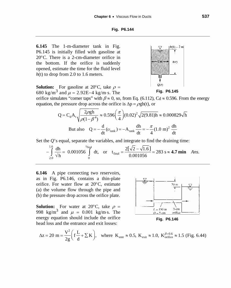
Chapter 6 • Viscous Flow in Ducts 537
Fig. P6.144
6.145 The 1-m-diameter tank in Fig. P6.145 is initially filled with gasoline at 20°C. There is a 2-cm-diameter orifice in the bottom. If the orifice is suddenly opened, estimate the time for the fluid level h(t) to drop from 2.0 to 1.6 meters.
Solution: For gasoline at 20°C, take ρ = 680 kg/m3 and μ = 2.92E−4 kg/m⋅s. The
Fig. P6.145
orifice simulates “corner taps” with β ≈ 0, so, from Eq. (6.112), Cd ≈ 0.596. From the energy equation, the pressure drop across the orifice is Δp = ρgh(t), or
2d t 4
2 ghQ C A 0.596 (0.02) 2(9.81)h 0.000829 h4(1 )
ρ πρ β
⎛ ⎞= ≈ ≈⎜ ⎟⎝ ⎠−
2tank tank
d dhBut also Q ( ) A (1.0 m)dt dt 4 dt
dhπυ= − = − = −
Set the Q’s equal, separate the variables, and integrate to find the draining time: finalt1.6
final2.0 0
dh 2 2 1.6 0.001056 dt, or t 283 s0.001056h[ ] Ans.−
− = = = ≈√∫ ∫ 4.7 min
6.146 A pipe connecting two reservoirs, as in Fig. P6.146, contains a thin-plate orifice. For water flow at 20°C, estimate (a) the volume flow through the pipe and (b) the pressure drop across the orifice plate.
Solution: For water at 20°C, take ρ = 998 kg/m3 and μ = 0.001 kg/m⋅s. The energy equation should include the orifice head loss and the entrance and exit losses:
Fig. P6.146
20.6
entr exit orificeV Lz 20 m f K , where K 0.5, K 1.0, K 1.5 (Fig. 6.44)2g d
β=⎛ ⎞Δ = = + ∑ ≈ ≈ ≈⎜ ⎟⎝ ⎠
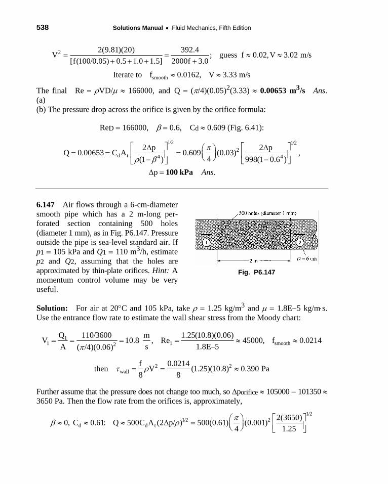
538 Solutions Manual • Fluid Mechanics, Fifth Edition
2
smooth
2(9.81)(20) 392.4V ; guess f 0.02,V 3.02 m/s[f(100/0.05) 0.5 1.0 1.5] 2000f 3.0
Iterate to f 0.0162, V 3.33 m/s
= = ≈+ + + +
≈ ≈
≈
The final Re = ρVD/μ ≈ 166000, and Q = (π/4)(0.05)2(3.33) ≈ 0.00653 m3/s Ans. (a) (b) The pressure drop across the orifice is given by the orifice formula:
ReD = 166000, β = 0.6, Cd ≈ 0.609 (Fig. 6.41):
1/2 1/222 p 2 pπ⎡ ⎤
d t 4 4Q 0.00653 C A 0.609 (0.03) ,4(1 ) 998(1 0.6 )
p Ans.ρ β
⎡ ⎤Δ Δ⎛ ⎞= = =⎢ ⎥ ⎜ ⎟ ⎢ ⎥⎝ ⎠− −⎣ ⎦⎣ ⎦Δ = 100 kPa
6.147 Air flows through a 6-cm-diameter smooth pipe which has a 2 m-long per-forated section containing 500 holes (diameter 1 mm), as in Fig. P6.147. Pressure outside the pipe is sea-level standard air. If p1 = 105 kPa and Q1 = 110 m3/h, estimate p2 and Q2, assuming that the holes are approximated by thin-plate orifices. Hint: A momentum control volume may be very useful.
Fig. P6.147
Solution: For air at 20°C and 105 kPa, take ρ = 1.25 kg/m3 and μ = 1.8E−5 kg/m⋅s. Use the entrance flow rate to estimate the wall shear stress from the Moody chart:
11 1 smooth2
Q 110/3600 m 1.25(10.8)(0.06)V 10.8 , Re 45000, f 0.0214A s 1.8E 5( /4)(0.06)π
= = = = ≈ ≈−
2 2wall
f 0.0214then V (1.25)(10.8) 0.390 Pa8 8
τ ρ= = ≈
Further assume that the pressure does not change too much, so Δporifice ≈ 105000 − 101350 ≈ 3650 Pa. Then the flow rate from the orifices is, approximately,
1/2
51/2 2
d d t2(3650)0, C 0.61: Q 500C A (2 p/ ) 500(0.61) (0.001)
4 1.2πβ ρ ⎛ ⎞ ⎡ ⎤≈ ≈ ≈ Δ = ⎜ ⎟ ⎢ ⎥⎝ ⎠ ⎣ ⎦
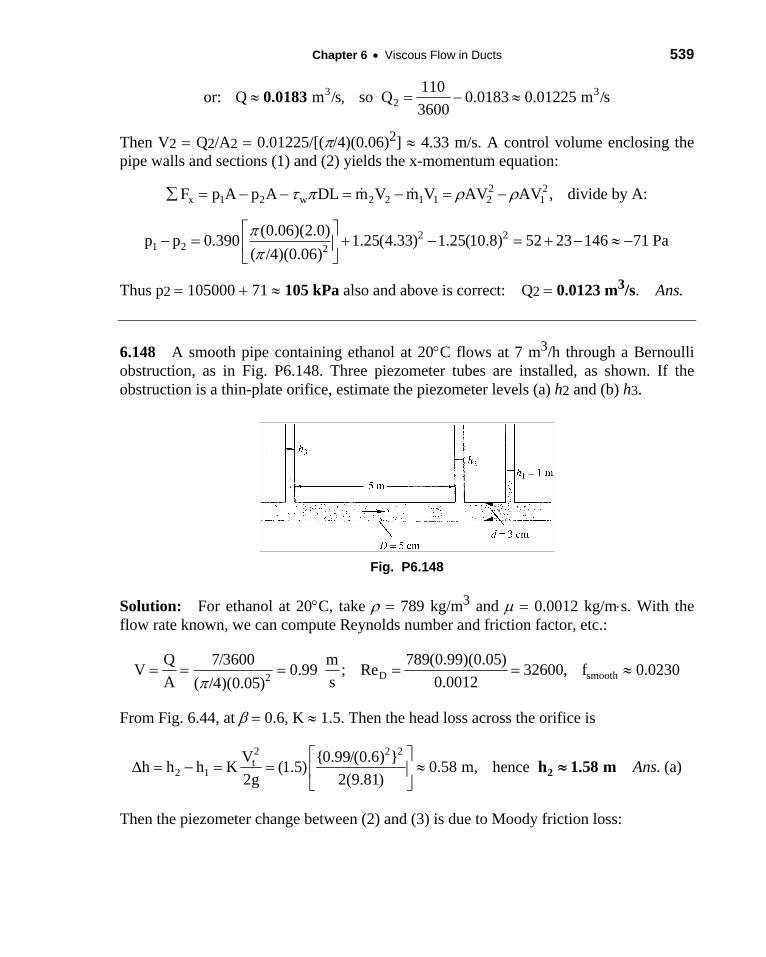
Chapter 6 • Viscous Flow in Ducts 539
3 32
110or: Q m /s, so Q 0.0183 0.01225 m /s3600
≈ = − ≈0.0183
Then V2 = Q2/A2 = 0.01225/[(π/4)(0.06)2] ≈ 4.33 m/s. A control volume enclosing the pipe walls and sections (1) and (2) yields the x-momentum equation:
2 2x 1 2 w 2 2 1 1 2 1F p A p A DL m V m V AV AV , divide by A:τ π ρ ρ∑ = − − = − = −
2 21 2 2
(0.06)(2.0)p p 0.390 1.25(4.33) 1.25(10.8) 52 23 146 71 Pa( /4)(0.06)ππ
⎡ ⎤− = + − = + − ≈ −⎢ ⎥
⎣ ⎦
Thus p2 = 105000 + 71 ≈ 105 kPa also and above is correct: Q2 = 0.0123 m3/s. Ans.
6.148 A smooth pipe containing ethanol at 20°C flows at 7 m3/h through a Bernoulli obstruction, as in Fig. P6.148. Three piezometer tubes are installed, as shown. If the obstruction is a thin-plate orifice, estimate the piezometer levels (a) h2 and (b) h3.
Fig. P6.148
Solution: For ethanol at 20°C, take ρ = 789 kg/m3 and μ = 0.0012 kg/m⋅s. With the flow rate known, we can compute Reynolds number and friction factor, etc.:
D smooth2Q 7/3600 m 789(0.99)(0.05)V 0.99 ; Re 32600, f 0.0230A s 0.0012( /4)(0.05)π
= = = = = ≈
From Fig. 6.44, at β = 0.6, K ≈ 1.5. Then the head loss across the orifice is
2 2 2t
2 1V {0.99/(0.6) }h h h K (1.5) 0.58 m, hence (a)2g 2(9.81)
Ans.⎡ ⎤
Δ = − = = ≈⎢ ⎥⎣ ⎦
≈2h 1.58 m
Then the piezometer change between (2) and (3) is due to Moody friction loss:

540 Solutions Manual • Fluid Mechanics, Fifth Edition 2 2L V 5 (0.99)⎛ ⎞− = = = =3 2 f
3
h h h f (0.023) 0.12 m,d 2g 0.05 2(9.81)
or h 1.58 0.12 (b)Ans.
⎜ ⎟⎝ ⎠
= + ≈ 1.7 m

Chapter 6 • Viscous Flow in Ducts 541
6.149 In a laboratory experiment, air at 20°C flows from a large tank through a 2-cm-diameter smooth pipe into a sea-level atmosphere, as in Fig. P6.149. The flow is metered by a long-radius nozzle of 1-cm diameter, using a manometer with Meriam red oil (SG = 0.827). The pipe is 8 m long. The measurements of tank pressure and manometer height are as follows:
Fig. P6.149
ptank, Pa (gage):
60 320 1200 2050 2470 3500 4900
hmano, mm: 6 38 160 295 380 575 820 Use this data to calculate the flow rates Q and Reynolds numbers ReD and make a plot of measured flow rate versus tank pressure. Is the flow laminar or turbulent? Compare the data with theoretical results obtained from the Moody chart, including minor losses. Discuss.
Solution: For air take ρ =1.2 kg/m3 and μ = 0.000015 kg/m⋅s. With no elevation change and negligible tank velocity, the energy equation would yield
2
tank 1 , 0.5 and 0.72atm entrance nozzle ent nozV Lp p f K K K K
Dρ ⎛ ⎞− = + + + ≈ ≈⎜ ⎟⎝ ⎠
Since Δp is given, we can use this expression plus the Moody chart to predict V and Q = AV and compare with the flow-nozzle measurements. The flow nozzle formula is:
42 where ( ) , from Fig. 6.42 and 0.5(1 )
manothroat d oil air d
pV C p gh Cρ ρ βρ β
Δ= Δ = −
−=
The friction factor is given by the smooth-pipe Moody formula, Eq. (6.48) for ε = 0. The results may be tabulated as follows, and the plot on the next page shows excellent (too good?) agreement with theory. ptank, Pa: 60 320 1200 2050 2470 3500 4900 V, m/s (nozzle data): 2.32 5.82 11.9 16.1 18.2 22.3 26.4 Q, m3/h (nozzle data): 2.39 6.22 12.9 17.6 19.9 24.5 29.1 Q, m3/h (theory): 2.31 6.25 13.3 18.0 20.0 24.2 28.9
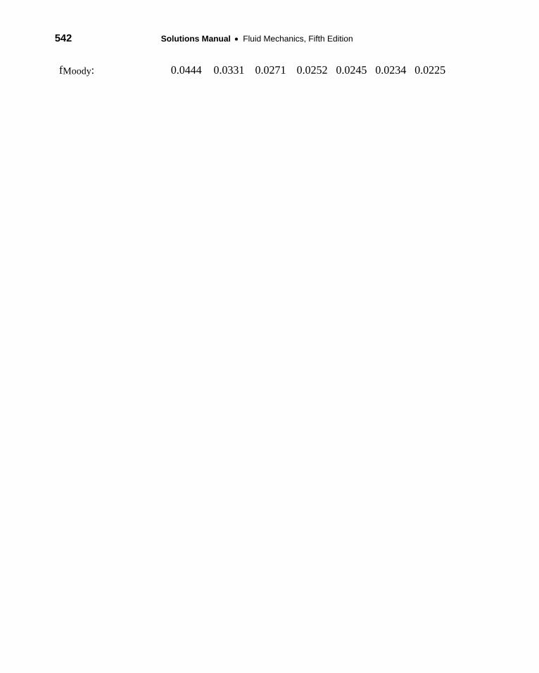
542 Solutions Manual • Fluid Mechanics, Fifth Edition
fMoody: 0.0444 0.0331 0.0271 0.0252 0.0245 0.0234 0.0225

Chapter 6 • Viscous Flow in Ducts 543
6.150 Gasoline at 20°C flows at 0.06 m3/s through a 15-cm pipe and is metered by a 9-cm-diameter long-radius flow nozzle (Fig. 6.40a). What is the expected pressure drop across the nozzle?
Solution: For gasoline at 20°C, take ρ = 680 kg/m and μ = 2.92E−4 kg/m⋅s. Calculate the pipe velocity and Reynolds number:
D2Q 0.06 m 680(3.40)(0.15)V 3.40 , Re 1.19E6A s 2.92E 4( /4)(0.15)π
= = = = ≈−
The ISO correlation for discharge (Eq. 6.114) is used to estimate the pressure drop: 1/2 1/26 6
dD
10 10 (0.6)C 0.9965 0.00653 0.9965 0.00653Re 1.19E6
0.9919β⎛ ⎞ ⎡ ⎤≈ − = − ≈⎜ ⎟ ⎢ ⎥
⎝ ⎠ ⎣ ⎦
2 2 pπ Δ⎛ ⎞4Then Q 0.06 (0.9919) (0.09) ,
4 680(1 0.6 )
Solve Ans.
= = ⎜ ⎟⎝ ⎠ −
≈Δp 27000 Pa

544 Solutions Manual • Fluid Mechanics, Fifth Edition
P6.151 An engineer needs to monitor a flow of 20°C gasoline at about 250±25 gal/min through a 4-in-diameter smooth pipe. She can use an orifice plate, a long-radius flow nozzle, or a venturi nozzle, all with 2-in-diameter throats. The only differential pressure gage available is accurate in the range 6 to 10 lbf/in2. Disregarding flow losses, which device is best?
Solution: For gasoline at 20°C, take ρ = 680 kg/m3 and μ = 2.92E-4 kg/m-s. We are given
β = 2/4 = 0.5. The flow rate is in the range 0.0142 < Q < 0.0174 m3/s. The pipe Reynolds number is in the range ReD = 460,000 ± 10%. In SI units, the throat diameter is 0.0508 m, and its area is (π/4)(0.0508m)2 = 0.00203 m2. Our basic “obstruction” formula is Eq. (6.104):
sm
mkgpmCpACQ dtd
3
432
4 0016.00158.0})5.0(1){/680(
2)00203.0()1(
2±=
−
Δ=
−
Δ=
βρ
It remains only to determine Cd for the three devices and then calculate Δp. The results are:
Orifice plate, D:1/2D taps: Cd ≈ 0.605 , Δp = 6.2 to 9.3 lbf/in2 Ans.
Long-radius flow nozzle: Cd ≈ 0.99 , Δp = 2.3 to 3.5 lbf/in2
Venturi nozzle: Cd ≈ 0.977 , Δp = 2.4 to 3.6 lbf/in2
Only the orifice plate, with its high losses, is compatible with the available pressure gage.
6.152 Kerosene at 20°C flows at 20 m3/h in an 8-cm-diameter pipe. The flow is to be metered by an ISA 1932 flow nozzle so that the pressure drop is 7 kPa. What is the proper nozzle diameter?
Chapter 6 • Viscous Flow in Ducts 545
Solution: For kerosene at 20°C, take ρ = 804 kg/m3 and μ =1.92E−3 kg/m⋅s. We cannot calculate the discharge coefficient exactly because we don’t know β, so just estimate Cd:
32
d 42(7000) 20 mGuess C 0.99, then Q 0.99 (0.08 )
4 3600 s804(1 )π β
β⎛ ⎞≈ ≈ =⎜ ⎟⎝ ⎠ −
2
4 1/2or: 0.268, solve 0.508,β β≈ ≈
D
(1 )
4(804)(20/3600)Re 37000(1.92E 3)(0.08)
β
π
−
= ≈−
Now compute a better Cd from the ISA nozzle correlation, Eq. (6.115): 1.156
4.1 4.7d
D
10C 0.99 0.2262 (0.000215 0.001125 0.00249 ) 0.9647Re
β β β⎛ ⎞
≈ − + − + ≈⎜ ⎟⎝ ⎠
Iterate once to obtain a better β ≈ 0.515, d = 0.515(8 cm) ≈ 4.12 cm Ans.

546 Solutions Manual • Fluid Mechanics, Fifth Edition
6.153 Two water tanks, each with base area of 1 ft2, are connected by a 0.5-in-diameter long-radius nozzle as in Fig. P6.153. If h = 1 ft as shown for t = 0, estimate the time for h(t) to drop to 0.25 ft.
Solution: For water at 20°C, take ρ = 1.94 slug/ft3 and μ = 2.09E−5 slug/ft⋅s. For a long-radius nozzle with β ≈ 0, guess Cd ≈ 0.98 and Kloss ≈ 0.9 from Fig. 6.44. The elevation difference h must balance the head losses in the nozzle and submerged exit:
Fig. P6.153
2 2t t
loss nozzle exit tV Vz h K (0.9 1.0 ) h, solve V 5.82 h2g 2(32.2)
Δ = ∑ = ∑ = + = =
2
ankt t1/2 dh dhhence Q V 0.00794 h A 0.5
4 12 dt dtπ⎛ ⎞ ⎛ ⎞= ≈ = − = −⎜ ⎟ ⎜ ⎟⎝ ⎠ ⎝ ⎠
12
The boldface factor 1/2 accounts for the fact that, as the left tank falls by dh, the right tank rises by the same amount, hence dh/dt changes twice as fast as for one tank alone. We can separate and integrate and find the time for h to drop from 1 ft to 0.25 ft:
( )finalt1.0 2 1 0.25final
0.25 0
dh 0.0159 dt, or: t 0.0159h
Ans.= = ≈∫ ∫ 63 s−
6.154 Water at 20°C flows through the orifice in the figure, which is monitored by a mercury manometer. If d = 3 cm, (a) what is h when the flow is 20 m3/h; and (b) what is Q when h = 58 cm?
Solution: (a) Evaluate V = Q/A = 2.83 m/s and ReD = ρVD/μ = 141,000, β = 0.6, thus Cd ≈ 0.613.
Fig. P6.154
2 24 4
20 2 2(13550 998)(9.81)(0.613) (0.03)3600 4 4(1 ) 998(1 0.6 )d
p hQ C dπ πρ β
Δ −= = =
− −
where we have introduced the manometer formula Δp = (ρmercury − ρwater)gh.
Solve for: 0.58 m (a)Ans.≈ =h 58 cm
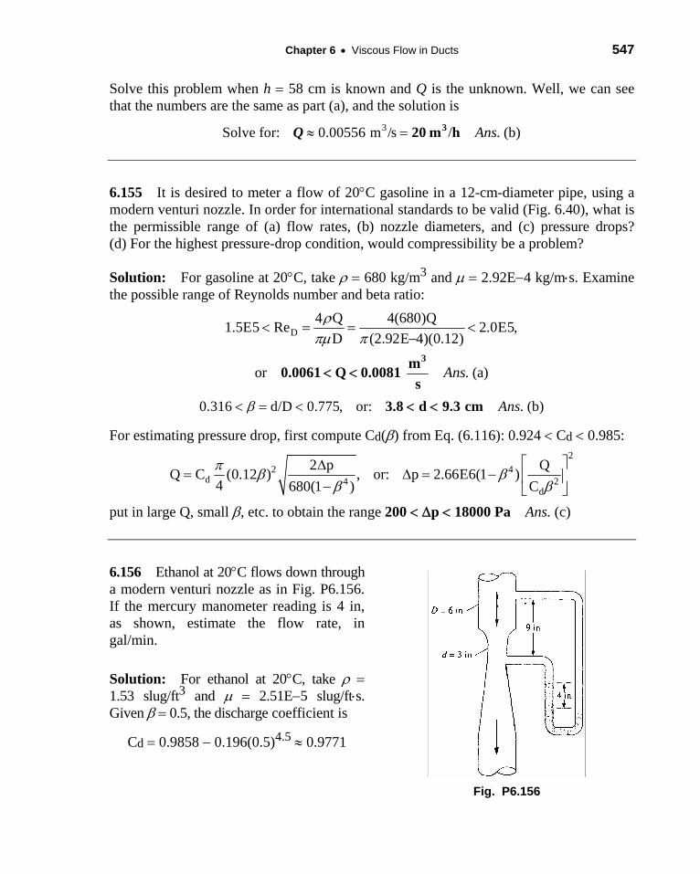
Chapter 6 • Viscous Flow in Ducts 547
Solve this problem when h = 58 cm is known and Q is the unknown. Well, we can see that the numbers are the same as part (a), and the solution is
3Solve for: 0.00556 m /s / (b)Ans.≈ =Q 320 m h
6.155 It is desired to meter a flow of 20°C gasoline in a 12-cm-diameter pipe, using a modern venturi nozzle. In order for international standards to be valid (Fig. 6.40), what is the permissible range of (a) flow rates, (b) nozzle diameters, and (c) pressure drops? (d) For the highest pressure-drop condition, would compressibility be a problem?
Solution: For gasoline at 20°C, take ρ = 680 kg/m3 and μ = 2.92E−4 kg/m⋅s. Examine the possible range of Reynolds number and beta ratio:
D4 Q 4(680)Q1.5E5 Re 2.0E5,
D (2.92E 4)(0.12)
or (a)Ans.
ρπμ π −
< <3m0.0061 Q 0.0081
s
< = = <
0.316 d/D 0.775, or: (b)Ans.β< = < 3.8 d 9.3 cm< <
For estimating pressure drop, first compute Cd(β) from Eq. (6.116): 0.924 < Cd < 0.985: 2
−2 4d 4 2
d
2 p QQ C (0.12 ) , or: p 2.66E6(1 )4 680(1 ) Cπ β β
β β⎡ ⎤Δ
= Δ = ⎢ ⎥− ⎣ ⎦
put in large Q, small β, etc. to obtain the range 200 < Δp < 18000 Pa Ans. (c)
6.156 Ethanol at 20°C flows down through a modern venturi nozzle as in Fig. P6.156. If the mercury manometer reading is 4 in, as shown, estimate the flow rate, in gal/min.
Solution: For ethanol at 20°C, take ρ = 1.53 slug/ft3 and μ = 2.51E−5 slug/ft⋅s. Given β = 0.5, the discharge coefficient is
Cd = 0.9858 − 0.196(0.5)4.5 ≈ 0.9771
Fig. P6.156
548 Solutions Manual • Fluid Mechanics, Fifth Edition
The 9-inch displacement of manometer taps does not affect the pressure drop reading, because both legs are filled with ethanol. Therefore we proceed directly to Δp and Q:
2nozzle merc ethp ( )gh (26.3 1.53)(32.2)(4/12) 266 lbf/ftρ ρΔ = − = − ≈
1/2 2
d t 4 42 p 3 2(266) ftHence Q C A 0.9771
4 12 s(1 ) 1.53(1 0.5 )Ans.π
ρ β⎡ ⎤Δ ⎛ ⎞⎛ ⎞= = ≈⎜ ⎟⎜ ⎟⎢ ⎥− −⎝ ⎠⎝ ⎠⎣ ⎦
3
0.924
6.157 Modify Prob. 6.156 if the fluid is air at 20°C, entering the venturi at a pressure of 18 psia. Should a compressibility correction be used?
Solution: For air at 20°C and 18 psi, take ρ = 0.00286 slug/ft3 and μ = 3.76E−7 slug/ft⋅s. With β still equal to 0.5, Cd still equals 0.9771 as previous page. The manometer reading is
2nozzlep (26.3 0.00286)(32.2)(4/12) 282 lbf/ft ,Δ = − ≈
2 3
43 2(282)whence Q 0.9771
4 12 0.00286(1 0.5 )Ans.π⎛ ⎞⎛ ⎞= ≈⎜ ⎟⎜ ⎟ −⎝ ⎠⎝ ⎠
ft22.0s
From this result, the throat velocity Vt = Q/At ≈ 448 ft/s, quite high, the Mach number in the throat is approximately Ma = 0.4, a (slight) compressibility correction might be expected. [Making a one-dimensional subsonic-flow correction, using the methods of Chap. 9, results in a throat volume flow estimate of Q ≈ 22.8 ft3/s, about 4% higher.]
6.158 Water at 20°C flows in a long horizontal commercial-steel 6-cm-diameter pipe which contains a classical Herschel venturi with a 4-cm throat. The venturi is connected to a mercury manometer whose reading is h = 40 cm. Estimate (a) the flow rate, in m3/h, and (b) the total pressure difference between points 50 cm upstream and 50 cm downstream of the venturi.
Solution: For water at 20°C, take ρ = 998 kg/m3 and μ = 0.001kg/m⋅s. For commercial steel, ε ≈ 0.046 mm, hence ε/d = 0.046/60 = 0.000767. First estimate the flow rate:
m wp ( )gh (13560 998)(9.81)(0.40) 49293 Paρ ρΔ = − = − ≈ 3
2d 4
2(49293) mGuess C 0.985, Q (0.985) (0.04) 0.0137 π⎛ ⎞≈ = ≈⎜ ⎟
D
4 s998[1 (4/6) ]
4 QCheck Re 291000D
ρπμ
−⎝ ⎠
= ≈
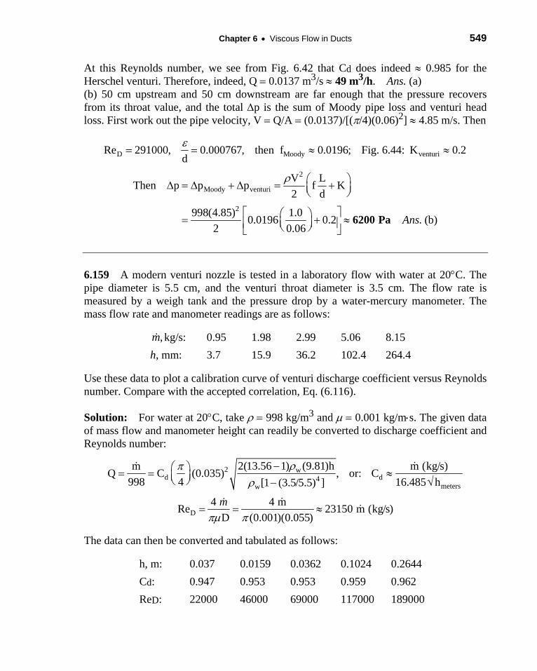
Chapter 6 • Viscous Flow in Ducts 549
At this Reynolds number, we see from Fig. 6.42 that Cd does indeed ≈ 0.985 for the Herschel venturi. Therefore, indeed, Q = 0.0137 m3/s ≈ 49 m3/h. Ans. (a) (b) 50 cm upstream and 50 cm downstream are far enough that the pressure recovers from its throat value, and the total Δp is the sum of Moody pipe loss and venturi head loss. First work out the pipe velocity, V = Q/A = (0.0137)/[(π/4)(0.06)2] ≈ 4.85 m/s. Then
D Moody venturiRe 291000, 0.000767, then f 0.0196; Fig. 6.44: K 0.2dε
= = ≈ ≈
2
Moody venturi
2
V LThen p p p f K2 d
998(4.85) 1.00.0196 0.2 (b)2 0.06
Ans.
ρ ⎛ ⎞Δ = Δ + Δ = +⎜ ⎟⎝ ⎠
⎡ ⎤⎛ ⎞= + ≈⎜ ⎟⎢ ⎥⎝ ⎠⎣ ⎦6200 Pa
6.159 A modern venturi nozzle is tested in a laboratory flow with water at 20°C. The pipe diameter is 5.5 cm, and the venturi throat diameter is 3.5 cm. The flow rate is measured by a weigh tank and the pressure drop by a water-mercury manometer. The mass flow rate and manometer readings are as follows:
,m kg/s: 0.95 1.98 2.99 5.06 8.15 h, mm: 3.7 15.9 36.2 102.4 264.4
Use these data to plot a calibration curve of venturi discharge coefficient versus Reynolds number. Compare with the accepted correlation, Eq. (6.116).
Solution: For water at 20°C, take ρ = 998 kg/m3 and μ = 0.001 kg/m⋅s. The given data of mass flow and manometer height can readily be converted to discharge coefficient and Reynolds number:
2 wd d4
metersw
2(13.56 1) (9.81)hm mQ C (0.035) , or: C998 4 16.485 h[1 (3.5/5.5) ]
ρπρ
−⎛ ⎞= = ≈⎜ ⎟⎝ ⎠ √− (kg/s)
D4 4 mRe 23150 m (kg/s)
D (0.001)(0.055)m
πμ π= = ≈
The data can then be converted and tabulated as follows:
h, m: 0.037 0.0159 0.0362 0.1024 0.2644 Cd: 0.947 0.953 0.953 0.959 0.962 ReD: 22000 46000 69000 117000 189000
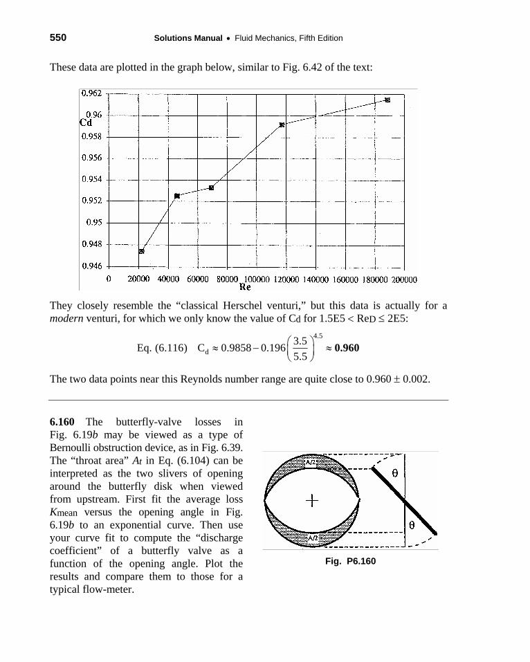
550 Solutions Manual • Fluid Mechanics, Fifth Edition
These data are plotted in the graph below, similar to Fig. 6.42 of the text:
They closely resemble the “classical Herschel venturi,” but this data is actually for a modern venturi, for which we only know the value of Cd for 1.5E5 < ReD ≤ 2E5:
4.5
d3.5Eq. (6.116) C 0.9858 0.1965.5
⎛ ⎞≈ − ≈⎜ ⎟⎝ ⎠
0.960
The two data points near this Reynolds number range are quite close to 0.960 ± 0.002.
6.160 The butterfly-valve losses in Fig. 6.19b may be viewed as a type of Bernoulli obstruction device, as in Fig. 6.39. The “throat area” At in Eq. (6.104) can be interpreted as the two slivers of opening around the butterfly disk when viewed from upstream. First fit the average loss Kmean versus the opening angle in Fig. 6.19b to an exponential curve. Then use your curve fit to compute the “discharge coefficient” of a butterfly valve as a function of the opening angle. Plot the results and compare them to those for a typical flow-meter.
Fig. P6.160

Chapter 6 • Viscous Flow in Ducts 551
Solution: The two “slivers” referred to are shown. The total sliver area equals total area reduced by a cosine factor:
2sliver total totalA A (1 cos ), where A R , R valve and pipe radiusθ π= − = =
The “effective” velocity passing through the slivers may be computed from continuity:
pipe pipetotaleff
slivers total slivers s t
V VAQ QVA A A A /A (1 cos )θ
= = = =−
Then the problem suggests that the loss coefficients might correlate better (and not vary so much or be so large as in Fig. 6.19b) if the loss is based on effective velocity:
2
(1 cos )pipe 2loss lossbetter Fig.6.192 2
effeff pipe
Vh hK KVV /2g V /2g
θ⎛ ⎞
= = = −⎜ ⎟⎝ ⎠
So we take the data for traditional “K” in Fig. 6.19b, multiply it by (1−cosθ)2, and replot it below. Actually, we have taken three exponential curve-fits, one for each manufacturer’s data shown in Fig. 6.19, to give an idea of the data uncertainty:
0.109 0.091 0.1121 2 3#1: K 3500 e ; 2: K 930 e ; # 3: K 2800 e , in degreesθ θ θ θ− − −≈ ≈ ≈
The calculations are made and are shown plotted below. This idea works fairly well, but the K’s still vary a bit over the range of θ. However, all K’s are now of order unity, which is a better correlation than the huge variations shown in Fig. 6.19b.
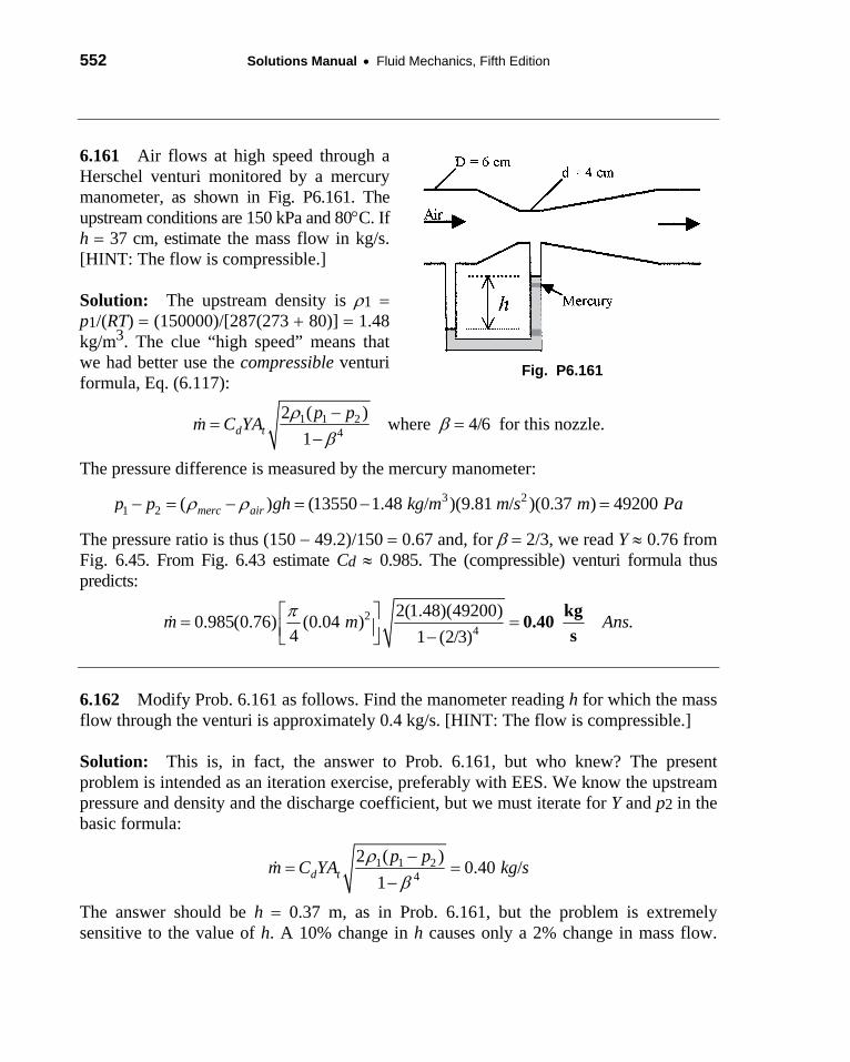
552 Solutions Manual • Fluid Mechanics, Fifth Edition
6.161 Air flows at high speed through a Herschel venturi monitored by a mercury manometer, as shown in Fig. P6.161. The upstream conditions are 150 kPa and 80°C. If h = 37 cm, estimate the mass flow in kg/s. [HINT: The flow is compressible.]
Solution: The upstream density is ρ1 = p1/(RT) = (150000)/[287(273 + 80)] = 1.48 kg/m3. The clue “high speed” means that we had better use the compressible venturi formula, Eq. (6.117):
Fig. P6.161
1 1 24
2 ( ) where 4/6 for this nozzle.1d t
p pm C YA ρ ββ−
= =−
The pressure difference is measured by the mercury manometer: 3 2
1 2 ( ) (13550 1.48 / )(9.81 / )(0.37 ) 49200 merc airp p gh kg m m s mρ ρ− = − = − = Pa
The pressure ratio is thus (150 − 49.2)/150 = 0.67 and, for β = 2/3, we read Y ≈ 0.76 from Fig. 6.45. From Fig. 6.43 estimate Cd ≈ 0.985. The (compressible) venturi formula thus predicts:
24
2(1.48)(49200)0.985(0.76) (0.04 ) 4 1 (2/3)
m mπ⎡ ⎤= =⎢ ⎥ −⎣ ⎦kg0.40s
Ans.
6.162 Modify Prob. 6.161 as follows. Find the manometer reading h for which the mass flow through the venturi is approximately 0.4 kg/s. [HINT: The flow is compressible.]
Solution: This is, in fact, the answer to Prob. 6.161, but who knew? The present problem is intended as an iteration exercise, preferably with EES. We know the upstream pressure and density and the discharge coefficient, but we must iterate for Y and p2 in the basic formula:
1 1 24
2 ( ) 0.40 /1d t
p pm C YA kg sρβ−
= =−
The answer should be h = 0.37 m, as in Prob. 6.161, but the problem is extremely sensitive to the value of h. A 10% change in h causes only a 2% change in mass flow.
Chapter 6 • Viscous Flow in Ducts 553
The actual answer to Prob. 6.161 was a mass flow of 0.402 kg/s. EES reports that, for mass flow exactly equal to 0.400 kg/s, the required manometer height is h = 0.361 m. Ans.
FUNDAMENTALS OF ENGINEERING EXAM PROBLEMS: Answers
FE 6.1 In flow through a straight, smooth pipe, the diameter Reynolds number for transition to turbulence is generally taken to be
(a) 1500 (b) 2300 (c) 4000 (d) 250,000 (e) 500,000 FE 6.2 For flow of water at 20°C through a straight, smooth pipe at 0.06 m3/h, the pipe diameter for which transition to turbulence occurs is approximately
(a) 1.0 cm (b) 1.5 cm (c) 2.0 cm (d) 2.5 cm (e) 3.0 cm FE 6.3 For flow of oil (μ = 0.1 kg/(m⋅s), SG = 0.9) through a long, straight, smooth 5-cm-diameter pipe at 14 m3/h, the pressure drop per meter is approximately
(a) 2200 Pa (b) 2500 Pa (c) 10,000 Pa (d) 160 Pa (e) 2800 Pa FE 6.4 For flow of water at a Reynolds number of 1.03E6 through a 5-cm-diameter pipe of roughness height 0.5 mm, the approximate Moody friction factor is
(a) 0.012 (b) 0.018 (c) 0.038 (d) 0.049 (e) 0.102 FE 6.5 Minor losses through valves, fittings, bends, contractions etc. are commonly modeled as proportional to
(a) total head (b) static head (c) velocity head (d) pressure drop (e) velocity FE 6.6 A smooth 8-cm-diameter pipe, 200 m long, connects two reservoirs, containing water at 20°C, one of which has a surface elevation of 700 m and the other with its surface elevation at 560 m. If minor losses are neglected, the expected flow rate through the pipe is
(a) 0.048 m3/h (b) 2.87 m3/h (c) 134 m3/h (d) 172 m3/h (e) 385 m3/h FE 6.7 If, in Prob. FE 6.6 the pipe is rough and the actual flow rate is 90 m3/hr, then the expected average roughness height of the pipe is approximately
(a) 1.0 mm (b) 1.25 mm (c) 1.5 mm (d) 1.75 mm (e) 2.0 mm FE 6.8 Suppose in Prob. FE 6.6 the two reservoirs are connected, not by a pipe, but by a sharp-edged orifice of diameter 8 cm. Then the expected flow rate is approximately
(a) 90 m3/h (b) 579 m3/h (c) 748 m3/h (d) 949 m3/h (e) 1048 m3/h FE 6.9 Oil (μ = 0.1 kg/(m⋅s), SG = 0.9) flows through a 50-m-long smooth 8-cm-diameter pipe. The maximum pressure drop for which laminar flow is expected is approximately
(a) 30 kPa (b) 40 kPa (c) 50 kPa (d) 60 kPa (e) 70 kPaFE 6.10 Air at 20°C and approximately 1 atm flows through a smooth 30-cm-square duct at 1500 cubic feet per minute. The expected pressure drop per meter of duct length is
(a) 1.0 Pa (b) 2.0 Pa (c) 3.0 Pa (d) 4.0 Pa (e) 5.0 Pa
554 Solutions Manual • Fluid Mechanics, Fifth Edition
FE 6.11 Water at 20°C flows at 3 cubic meters per hour through a sharp-edged 3-cm-diameter orifice in a 6-cm-diameter pipe. Estimate the expected pressure drop across the orifice.
(a) 440 Pa (b) 680 Pa (c) 875 Pa (d) 1750 Pa (e) 1870 Pa FE 6.12 Water flows through a straight 10-cm-diameter pipe at a diameter Reynolds number of 250,000. If the pipe roughness is 0.06 mm, what is the approximate Moody friction factor?
(a) 0.015 (b) 0.017 (c) 0.019 (d) 0.026 (e) 0.032 FE 6.13 What is the hydraulic diameter of a rectangular air-ventilation duct whose cross-section is 1 meter by 25 cm?
(a) 25 cm (b) 40 cm (c) 50 cm (d) 75 cm (e) 100 cm FE 6.14 Water at 20°C flows through a pipe at 300 gal/min with a friction head loss of 45 ft. What is the power required to drive this flow?
(a) 0.16 kW (b) 1.88 kW (c) 2.54 kW (d) 3.41 kW (e) 4.24 kW FE 6.15 Water at 20°C flows at 200 gal/min through a pipe 150 m long and 8 cm in diameter. If the friction head loss is 12 m, what is the Moody friction factor?
(a) 0.010 (b) 0.015 (c) 0.020 (d) 0.025 (e) 0.030
Chapter 6 • Viscous Flow in Ducts 555
COMPREHENSIVE PROBLEMS
C6.1 A pitot-static probe will be used to measure the velocity distribution in a water tunnel at 20°C. The two pressure lines from the probe will be connected to a U-tube manometer which uses a liquid of specific gravity 1.7. The maximum velocity expected in the water tunnel is 2.3 m/s. Your job is to select an appropriate U-tube from a manufacturer which supplies manometers of heights 8, 12, 16, 24 and 36 inches. The cost increases significantly with manometer height. Which of these should you purchase?
Solution: The pitot-static tube formula relates velocity to the difference between stagnation pressure po and static pressure ps in the water flow:
ρ ρ− = = =23
1 kg, where 998 and 2.3 2 smo s w w maxp p V V m
Meanwhile, the manometer reading h relates this pressure difference to the two fluids:
2 2(2.3)Solve for 0.385 ( 1) 2(9.81)(1.7 1)
maxmax
mano
Vh m2g SG
= = = =− −
15.2 in
( ) ( 1)o s mano w w manop p gh SG ghρ ρ ρ− = − = −
It would therefore be most economical to buy the 16-inch manometer. But be careful when you use it: a bit of overpressure will pop the manometer fluid out of the tube!
C6.2 A pump delivers a steady flow of water (ρ,μ) from a large tank to two other higher-elevation tanks, as shown. The same pipe of diameter d and roughness ε is used throughout. All minor losses except through the valve are neglected, and the partially-closed valve has a loss coefficient Kvalve. Turbulent flow may be assumed with all kinetic energy flux correction coefficients equal to 1.06. The pump net head H is a known function of QA and hence also of VA = QA/Apipe, for example, where a and b are constants. Subscript J refers to the junction point at the tee where branch A splits into B and C. Pipe length L
2AH a bV= − ,
C is much longer than LB. It is desired to predict the pressure at J, the three pipe velocities and friction factors, and the pump head. Thus there are 8 variables: H, VA, VB, VC, fA, fB, fC, pJ. Write down the eight equations needed to resolve this problem, but do not solve, since an elaborate iteration procedure, or an equation solver such as EES, would be required.
Solution: First, equation (1) is clearly the pump performance:
(1) 2AH a bV= −
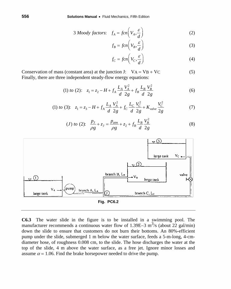
556 Solutions Manual • Fluid Mechanics, Fifth Edition
3 : ,A AMoody factors f fcn Vdε⎛= ⎜⎝
⎞⎟⎠
(2)
,B Bf fcn Vdε⎛= ⎜⎝
⎞⎟⎠
(3)
,C Cf fcn Vdε⎛= ⎜⎝
⎞⎟⎠
(4)
Conservation of mass (constant area) at the junction J: VA = VB + VC (5) Finally, there are three independent steady-flow energy equations:
2 2
1 2(1) (2):2 2
A A BA B
L V L Vto z z H f fd g d g
= − + + B (6)
2 22
2e1 3(1) (3):2 2
C C CA AA C valv
L V VL Vto z z H f f Kd g d g g
= − + + + (7)
2
2( ) (2):2
J atm B BJ B
p p L VJ to z z fg g dρ ρ
+ = + +g
(8)
Fig. PC6.2
C6.3 The water slide in the figure is to be installed in a swimming pool. The manufacturer recommends a continuous water flow of 1.39E−3 m3/s (about 22 gal/min) down the slide to ensure that customers do not burn their bottoms. An 80%-efficient pump under the slide, submerged 1 m below the water surface, feeds a 5-m-long, 4-cm-diameter hose, of roughness 0.008 cm, to the slide. The hose discharges the water at the top of the slide, 4 m above the water surface, as a free jet. Ignore minor losses and assume α = 1.06. Find the brake horsepower needed to drive the pump.

Chapter 6 • Viscous Flow in Ducts 557
Fig. PC6.3
Solution: For water take ρ = 998 kg/m3 and μ = 0.001 kg/m⋅s. Write the steady-flow energy equation from the water surface (1) to the outlet (2) at the top of the slide:
2 2 ms
1 1 2 21 2 2 2
1.39 3, where 1.106 2 2 (0.02)
a af pump
p pV V Ez z h h Vg g g g
α αρ ρ π
−+ + = + + + − = =
22
2 1 2( )2pumpV LSolve for h z z f
g dα⎛ ⎞= − + +⎜ ⎟⎝ ⎠
Work out Red = ρVd/μ = (998)(1.106)(0.04)/0.001 = 44200, ε/d = 0.008/4 = 0.002, whence fMoody = 0.0268. Use these numbers to evaluate the pump head above:
⎡ ⎤⎛ ⎞= − + + =⎜ ⎟⎢ ⎥⎝ ⎠⎣ ⎦
(1.106) 5.0(5.0 1.0) 1.06 0.0268 4.27 m,2(9.81) 0.04pumph
2
998(9.81)(1.39 3)(4.27)whence 0.8
pumpgQh E Ans.ρ
η−
= = =requiredBHP 73 watts
C6.4 Suppose you build a house out in the ‘boonies,’ where you need to run a pipe to the nearest water supply, which fortunately is about 1 km above the elevation of your house. The gage pressure at the water supply is 1 MPa. You require a minimum of 3 gal/min when your end of the pipe is open to the atmosphere. To minimize cost, you want to buy the smallest possible diameter pipe with an extremely smooth surface. (a) Find the total head loss from pipe inlet to exit, neglecting minor losses.
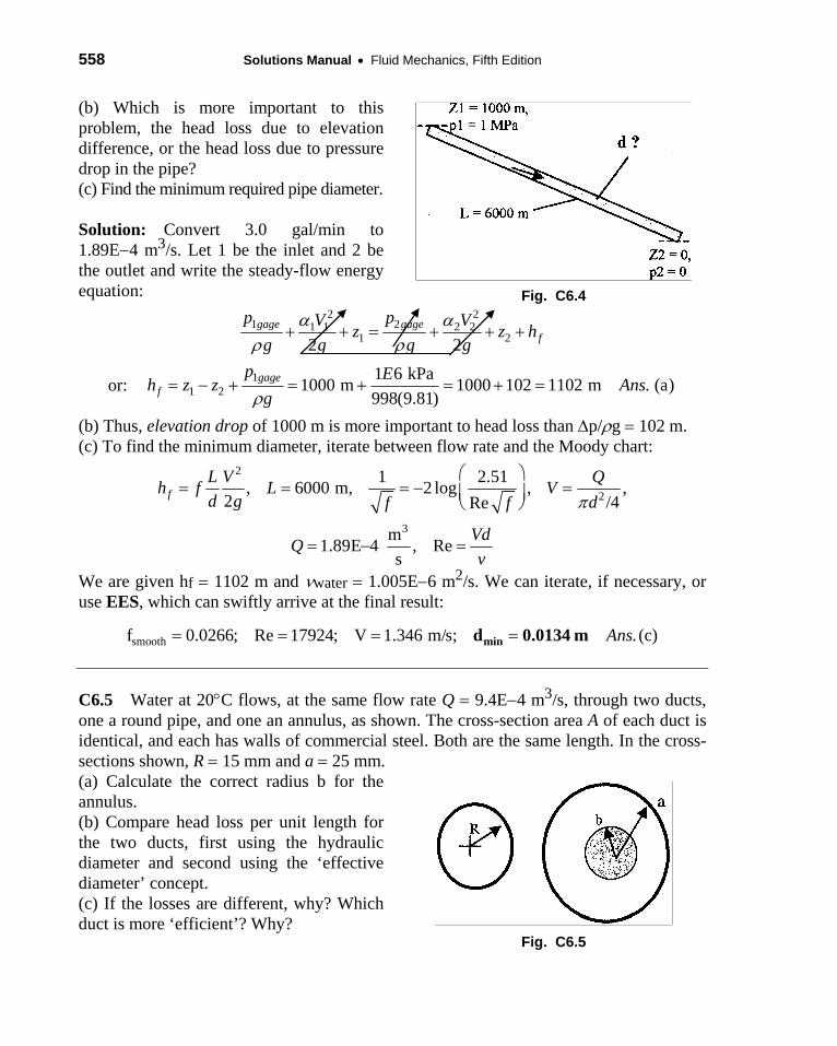
558 Solutions Manual • Fluid Mechanics, Fifth Edition
(b) Which is more important to this problem, the head loss due to elevation difference, or the head loss due to pressure drop in the pipe? (c) Find the minimum required pipe diameter.
Solution: Convert 3.0 gal/min to 1.89E−4 m3/s. Let 1 be the inlet and 2 be the outlet and write the steady-flow energy equation:
Fig. C6.4
2 21 2 2 2
1 22 2gage1 1gage
fp pV Vz z
g gα α
ρ ρ= + + + h
g g+ +
or: ρ
= − + = + = + =11 2
1 6 kPa1000 m 1000 102 1102 m (a)998(9.81)
gagef
p Eh z z Ans.g
(b) Thus, elevation drop of 1000 m is more important to head loss than Δp/ρg = 102 m. (c) To find the minimum diameter, iterate between flow rate and the Moody chart:
π⎝ ⎠
= − =3
2 /4Re
m1.89E 4 , Res
d g df f
VdQv
⎛ ⎞= = = − =⎜ ⎟
2
21 2.51, 6000 m, 2 log , ,f
L V Qh f L V
We are given hf = 1102 m and νwater = 1.005E−6 m2/s. We can iterate, if necessary, or use EES, which can swiftly arrive at the final result:
smoothf 0.0266; Re 17924; V 1.346 m/s; (c)Ans. = = = =mind 0.0134 m
C6.5 Water at 20°C flows, at the same flow rate Q = 9.4E−4 m3/s, through two ducts, one a round pipe, and one an annulus, as shown. The cross-section area A of each duct is identical, and each has walls of commercial steel. Both are the same length. In the cross-sections shown, R = 15 mm and a = 25 mm. (a) Calculate the correct radius b for the annulus. (b) Compare head loss per unit length for the two ducts, first using the hydraulic diameter and second using the ‘effective diameter’ concept. (c) If the losses are different, why? Which duct is more ‘efficient’? Why?
Fig. C6.5
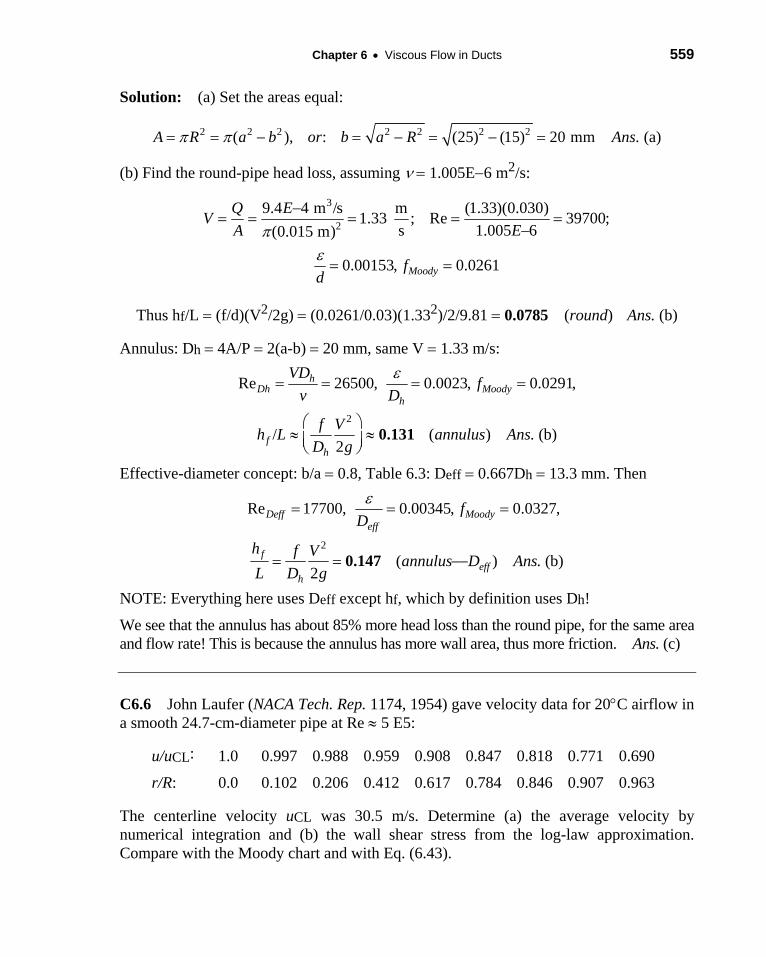
Chapter 6 • Viscous Flow in Ducts 559
Solution: (a) Set the areas equal:
π π= = − = − = − =2 2 2 2 2 2 2( ), : (25) (15) 20 mm (a)A R a b or b a R Ans.
(b) Find the round-pipe head loss, assuming ν = 1.005E−6 m2/s:
πε
−
= =
2 s 1.005 6(0.015 m)
0.00153, 0.0261Moody
A E
fd
−= = = = =
39.4 4 m /s m (1.33)(0.030)1.33 ; Re 39700;Q EV
Thus hf/L = (f/d)(V2/2g) = (0.0261/0.03)(1.332)/2/9.81 = 0.0785 (round) Ans. (b)
Annulus: Dh = 4A/P = 2(a-b) = 20 mm, same V = 1.33 m/s:
2/ ( )
2
h
fh
f Vh L annulus AnsD g
Re 26500, 0.0023, 0.0291,
. (b)
hDh Moody
VD fv D
ε= = = =
⎛ ⎞≈ ≈⎜ ⎟⎝ ⎠
0.131
Effective-diameter concept: b/a = 0.8, Table 6.3: Deff = 0.667Dh = 13.3 mm. Then
2
( )2
eff
feff
h
h f V annulus D AnsL D g
Re 17700, 0.00345, 0.0327,
. (b)
Deff MoodyfD
ε= = =
= = −−0.147
NOTE: Everything here uses Deff except hf, which by definition uses Dh!
We see that the annulus has about 85% more head loss than the round pipe, for the same area and flow rate! This is because the annulus has more wall area, thus more friction. Ans. (c)
C6.6 John Laufer (NACA Tech. Rep. 1174, 1954) gave velocity data for 20°C airflow in a smooth 24.7-cm-diameter pipe at Re ≈ 5 E5:
u/uCL: 1.0 0.997 0.988 0.959 0.908 0.847 0.818 0.771 0.690
r/R: 0.0 0.102 0.206 0.412 0.617 0.784 0.846 0.907 0.963
The centerline velocity uCL was 30.5 m/s. Determine (a) the average velocity by numerical integration and (b) the wall shear stress from the log-law approximation. Compare with the Moody chart and with Eq. (6.43).
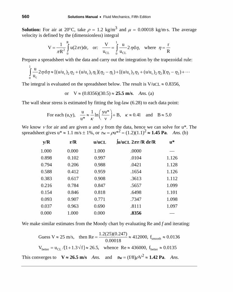
560 Solutions Manual • Fluid Mechanics, Fifth Edition
Solution: For air at 20°C, take ρ = 1.2 kg/m3 and μ = 0.00018 kg/m⋅s. The average velocity is defined by the (dimensionless) integral
R 1 rR
η =2CL CL0 0
1 V uV u(2 r)dr, or: 2 d , whereu uR
π η ηπ
= =∫ ∫
Prepare a spreadsheet with the data and carry out the integration by the trapezoidal rule: 1
+c 2 2 c 1 1 2 1 c 3 3 c 2 2 3 2c0
u 2 d [(u/u ) (u/u ) ]( ) [(u/u ) (u/u ) ]( )u
η η η η η η η η η η≈ + − + + −∫
The integral is evaluated on the spreadsheet below. The result is V/uCL ≈ 0.8356,
or V ≈ (0.8356)(30.5) ≈ 25.5 m/s. Ans. (a)
The wall shear stress is estimated by fitting the log-law (6.28) to each data point:
u 1 yu*For each (u,y), ln B, and B 5.0u*
κκ
⎛ ⎞≈ + ≈ 0.41⎜ ⎟⎝ ⎠ν≈
We know ν for air and are given u and y from the data, hence we can solve for u*. The spreadsheet gives u* ≈ 1.1 m/s ± 1%, or τw = ρu*2 = (1.2)(1.1)2 ≈ 1.45 Pa. Ans. (b)
y/R r/R u/uCL ∫u/uCL 2πr /R dr/R u*
1.000 0.000 1.000 .0000 — 0.898 0.102 0.997 .0104 1.126 0.794 0.206 0.988 .0421 1.128 0.588 0.412 0.959 .1654 1.126 0.383 0.617 0.908 .3613 1.112 0.216 0.784 0.847 .5657 1.099 0.154 0.846 0.818 .6498 1.101 0.093 0.907 0.771 .7347 1.098 0.037 0.963 0.690 .8111 1.097 0.000 1.000 0.000 .8356 —
We make similar estimates from the Moody chart by evaluating Re and f and iterating:
smooth
better CL better
Guess V 25 m/s, then Re 412000, f 0.01360.00018
V u /[1 1.3 f] 26.5, whence Re 436000, f 0.0135
≈ = ≈
= + √ ≈ ≈ ≈
1.2(25)(0.247)≈
This converges to V ≈ 26.5 m/s Ans. and τw = (f/8)ρV2 ≈ 1.42 Pa. Ans.
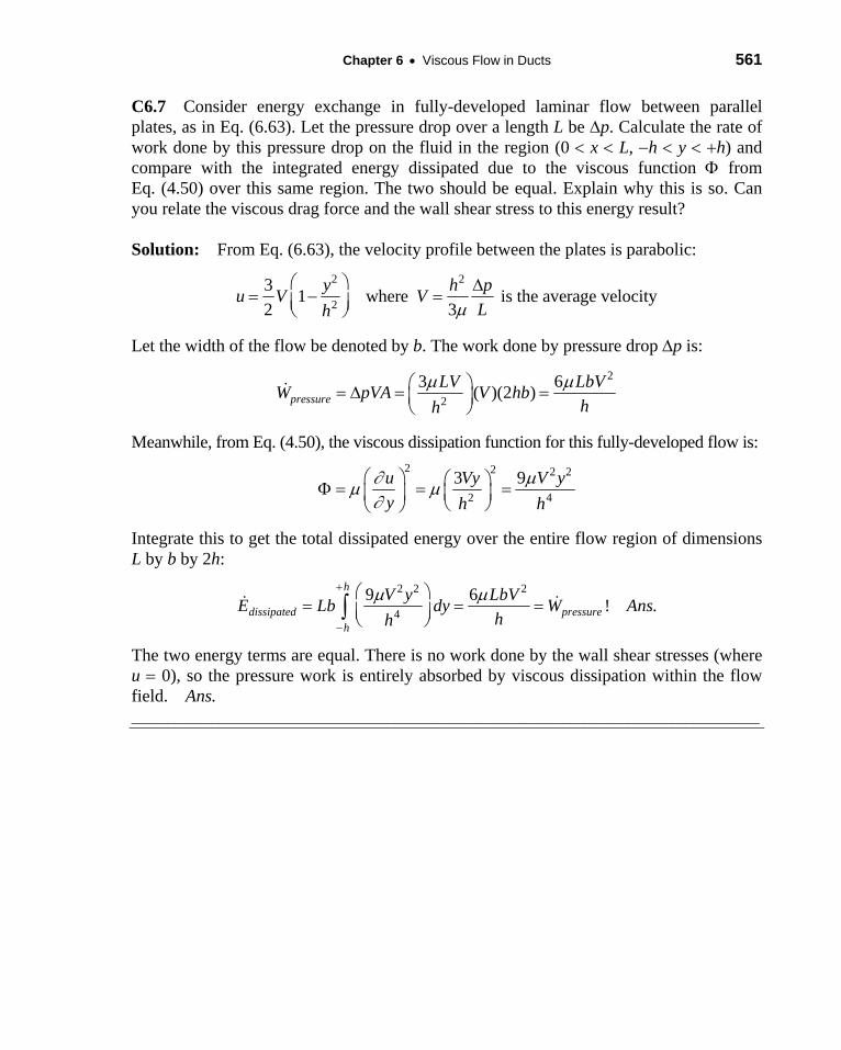
Chapter 6 • Viscous Flow in Ducts 561
C6.7 Consider energy exchange in fully-developed laminar flow between parallel plates, as in Eq. (6.63). Let the pressure drop over a length L be Δp. Calculate the rate of work done by this pressure drop on the fluid in the region (0 < x < L, −h < y < +h) and compare with the integrated energy dissipated due to the viscous function Φ from Eq. (4.50) over this same region. The two should be equal. Explain why this is so. Can you relate the viscous drag force and the wall shear stress to this energy result?
Solution: From Eq. (6.63), the velocity profile between the plates is parabolic: 2 2
23 1 where is the average velocity2 3
y h pu V VLh μ
⎛ ⎞ Δ= − =⎜ ⎟⎝ ⎠
Let the width of the flow be denoted by b. The work done by pressure drop Δp is: 2
23 6( )(2 )pressure
LV LbVW pVA V hbhh
μ μ⎛ ⎞= Δ = =⎜ ⎟⎝ ⎠
Meanwhile, from Eq. (4.50), the viscous dissipation function for this fully-developed flow is: 2 2 2 2y
2 43 9u Vy V
y h h∂ μμ μ∂
⎛ ⎞ ⎛ ⎞Φ = = =⎜ ⎟⎜ ⎟⎝ ⎠⎝ ⎠
Integrate this to get the total dissipated energy over the entire flow region of dimensions L by b by 2h:
2 2 2h
49 6 ! .dissipated pressure
h
V y LbVE Lb dy W Anshh
μ μ
−
⎛ ⎞= = =⎜ ⎟⎝ ⎠∫
+
The two energy terms are equal. There is no work done by the wall shear stresses (where u = 0), so the pressure work is entirely absorbed by viscous dissipation within the flow field. Ans. ______________________________________________________________________________________

562 Solutions Manual • Fluid Mechanics, Fifth Edition
C6.8 This text has presented the traditional correlations for turbulent smooth-wall friction
factor, Eq. (6.38), and the law-of-the-wall, Eq. (6.28). Recently, groups at Princeton and Oregon
[56] have made new friction measurements and suggest the following smooth-wall friction law:
537.0)Re(log930.1110 −= f
f D
In earlier work, they also report that better values for the constants κ and B in the log-law,
Eq. (6.28), are κ ≈ 0.421 ± 0.002 and B ≈ 5.62 ± 0.08. (a) Calculate a few values of f in the
range 1E4 ≤ ReD ≤ 1E8 and see how the two formulas differ. (b) Read Ref. 56 and briefly check
the five papers in its bibliography. Report to the class on the general results of this work.
Solution: The two formulas are practically identical except as the Reynolds number is
very high or very low. The new formula was fit to new, and extensive, friction data in
Ref. 56 and can thus be said to be slightly more accurate. Here is a table of calculations.
ReD fPrandtl f Ref.56 Difference 3000 0.04353 0.04251 -2.41% 10000 0.03089 0.0305 -1.10% 30000 0.02349 0.02344 -0.18% 100000 0.01799 0.01811 0.62% 300000 0.01447 0.01464 1.22% 1000000 0.01165 0.01186 1.76% 3.0E+06 0.009722 0.009938 2.17% 1.0E+07 0.008104 0.008316 2.56% 3.0E+07 0.006949 0.007153 2.86% 1.0E+08 0.005941 0.006134 3.15%
They differ by no more than 3%.