moac excel 2013 exam 77 420 - cabarrus county schools · table 5-1 lists common excel functions,...

115

Using Functions 5

KEY TERMS• argument

• AutoSum

• AVERAGE function

• COUNT function

• COUNTA function

• function

• MAX function

• MIN function

• NOW function

• PMT function

• SUBTOTAL function

• SUM function

• TODAY function

• trace arrow

LESSON SKILL MATRIX

Skills Exam Objective Objective Number

Exploring Functions

Displaying Dates and Times

with Functions

Summarizing Data with Functions Demonstrate how to apply the SUM function. 4.2.1

Demonstrate how to apply the COUNT function. 4.2.3

Demonstrate how to apply the AVERAGE function. 4.2.4

Demonstrate how to apply the MIN and MAX functions. 4.2.2

Using a Financial Function

Using Formulas to Create Subtotals

Uncovering Formula Errors

Displaying and Printing Formulas

©MCCAIG / iStockphoto

Demomomomonstratatate e hohohow to apply the MIN and MAX functions. 4

Lesson 5116

Creating and maintaining a personal budget requires more than simply estimating

and tracking expenses. You often want to see subtotals of certain data, for example,

to determine how much you spend quarterly. Sometimes you want to know your av-

erage payment per month for expenses that vary throughout the year. Budgets are

also working documents—they change over time and might require modifications

to the structure. Creating proper formulas builds flexibility into your worksheets.

Excel provides a wealth of predefined functions to help you enter formulas quickly

and accurately. In this lesson, you learn how to use simple Excel functions by work-

ing on an annual budget of household expenses.

SOFTWARE ORIENTATION

FORMULAS Tab

The FORMULAS tab in Excel 2013, shown in Figure 5-1, provides access to a library of formulas and functions. On this tab, you can use commands for quickly inserting functions, inserting totals, and displaying a visual map of cells that are dependent on a formula.

Insert Function AutoSum Function Library Trace Precedents

Insert Function button next to formula bar

Trace Dependents Evaluate Formula

In this lesson, you learn how to use a variety of simple functions to perform calculations in a budgeting worksheet. You also learn subtotaling techniques, how to work with formula errors, and how to print formulas.

Figure 5-1

The FORMULAS tab in Excel 2013

©MCCAIG / iStockphoto

ndndndnd f f funununctionsnsnsns. . On t t thihihis s tatab,b,b,b, youououou c c cananan use c c comommamandndndnds fofofofor r quququicklklklkly y y talslslsls, , , , ananand didididispspsplayiyiyiyingngngng a v v visisisual mamamap of cellslslsls thahat are e e e dededepepepependndndndenenent t t t on

AutooooSSSSum Funcncncnctitititiononon Libibibrarararyryry TrTrTracacace e e PrPrPrecedenenentstststs

Using Functions 117

EXPLORING FUNCTIONS

A function is a predefined formula that performs a calculation. Excel’s built-in functions are designed to perform different types of calculations—from simple to complex. When you apply a function to specific data, you eliminate the time involved in manually constructing a formula. Using functions ensures the accuracy of the formula’s results. You can type functions directly into Excel or use the tools on the FORMULAS tab to help you fill in formulas with the correct syntax.

STEP BY STEP Explore Functions

GET READY. LAUNCH Excel and open a new, blank workbook.

1. To become familiar with the tools available to build formulas and insert functions,

click the FORMULAS tab. Excel arranges functions by category in the Function Library

group, such as Financial, Logical, Text, and so on. Click the Financial button arrow to

display a drop-down list of functions (see Figure 5-2). If you create a financial function,

you can simply scroll through the list and select the function you want.

Figure 5-2

The Financial group menu of functions

2. You can also find a function using the Insert Function dialog box. On the FORMULAS

tab or on the formula bar, click the Insert Function button. The buttons are shown in

Figure 5-3.

Figure 5-3

The Insert Function buttonsInsert Function button

3. In the Insert Function dialog box, type a description of what you want to do. For

example, type date and click Go. Excel returns a list of functions that most closely

match your description (see Figure 5-4).

Bottom Line

Lesson 5118

Figure 5-4

The Insert Function dialog box displaying a list of functions in

response to your request

4. With DATE selected in the Select a function list, click OK. The Function Arguments

dialog box opens.

5. Enter the current year, the number of the current month, and the number of the current

day (see Figure 5-5). Click OK. The date is entered into the worksheet in cell A1.

Figure 5-5

Entering data into the Function Arguments dialog box

6. SAVE the workbook to your Lesson 5 folder as 05 Practice Solution.

PAUSE. LEAVE the workbook open to use in the next exercise.

Functions are a simplified way of entering formulas. The parameters of a function are called arguments. Each function name is followed by parentheses, which let Excel know where the ar-guments begin and end. Arguments appear within the parentheses and are performed from left to right. Depending on the function, an argument can be a constant value, a single-cell reference, a range of cells, or even another function. If a function contains multiple arguments, the arguments are separated by commas.

Even functions that require no arguments must still have parentheses following the name, as in =TODAY(). Table 5-1 lists common Excel functions, all of which are covered in this lesson.

Function Description Formula Syntax

AVERAGE Calculates the arithmetic mean, or

average, for the values in a range of

cells.

=AVERAGE(first value, second value,...)

MAX Analyzes an argument list to deter-

mine the highest value (the opposite

of the MIN function).

=MAX(first value, second value,...)

MIN Determines the smallest value of a

given list of numbers or arguments.

=MIN(first value, second value,...)

NOW Returns the current date and time. =NOW()

PMT Determines the payment for a loan

based on the interest rate of a loan,

the number of payments to be made,

and the loan amount.

=PMT(rate, nper, pv)

Table 5-1

Common Excel functions

Using Functions 119

Function Description Formula Syntax

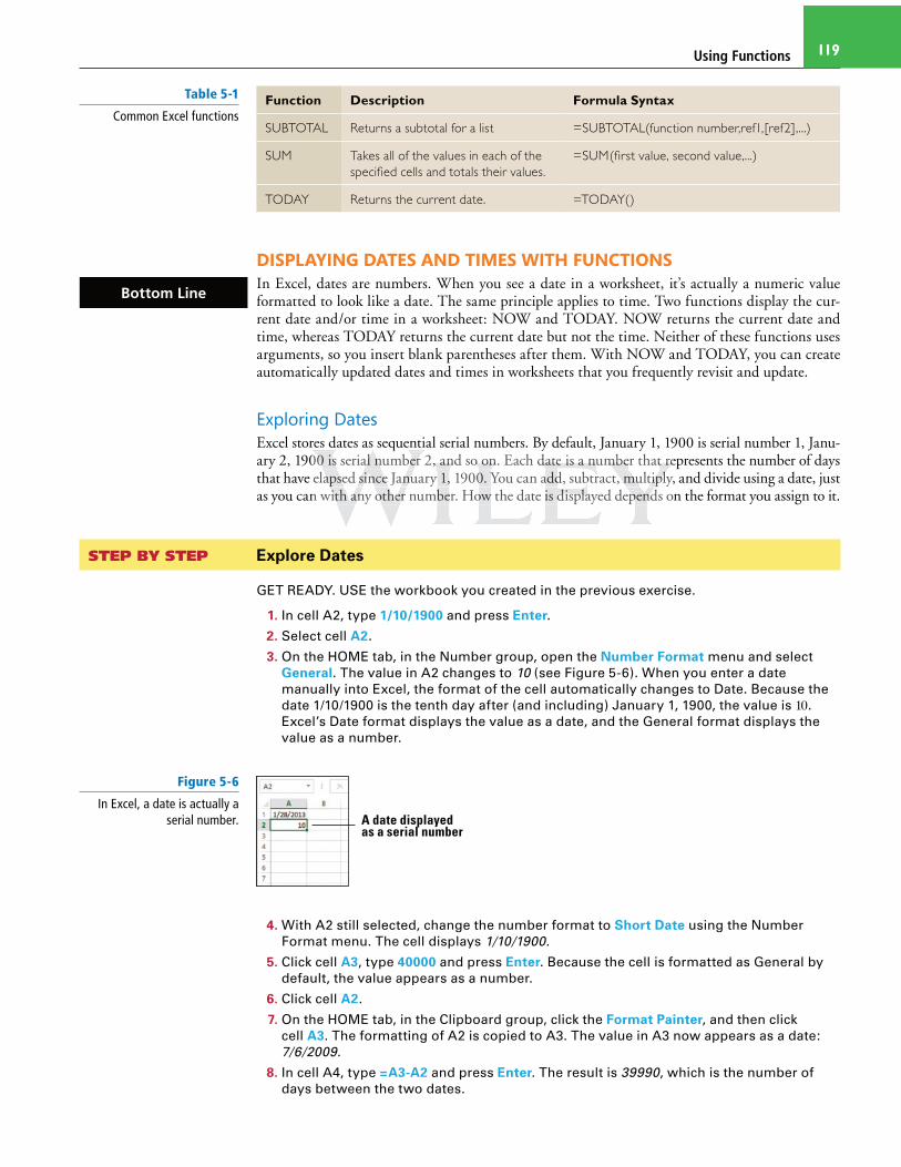
SUBTOTAL Returns a subtotal for a list =SUBTOTAL(function number,ref1,[ref2],...)

SUM Takes all of the values in each of the

specified cells and totals their values.

=SUM(first value, second value,...)

TODAY Returns the current date. =TODAY()

DISPLAYING DATES AND TIMES WITH FUNCTIONS

In Excel, dates are numbers. When you see a date in a worksheet, it’s actually a numeric value formatted to look like a date. The same principle applies to time. Two functions display the cur-rent date and/or time in a worksheet: NOW and TODAY. NOW returns the current date and time, whereas TODAY returns the current date but not the time. Neither of these functions uses arguments, so you insert blank parentheses after them. With NOW and TODAY, you can create automatically updated dates and times in worksheets that you frequently revisit and update.

Exploring Dates

Excel stores dates as sequential serial numbers. By default, January 1, 1900 is serial number 1, Janu-ary 2, 1900 is serial number 2, and so on. Each date is a number that represents the number of days that have elapsed since January 1, 1900. You can add, subtract, multiply, and divide using a date, just as you can with any other number. How the date is displayed depends on the format you assign to it.

STEP BY STEP Explore Dates

GET READY. USE the workbook you created in the previous exercise.

1. In cell A2, type 1/10/1900 and press Enter.

2. Select cell A2.

3. On the HOME tab, in the Number group, open the Number Format menu and select

General. The value in A2 changes to 10 (see Figure 5-6). When you enter a date

manually into Excel, the format of the cell automatically changes to Date. Because the

date 1/10/1900 is the tenth day after (and including) January 1, 1900, the value is .

Excel’s Date format displays the value as a date, and the General format displays the

value as a number.

Figure 5-6

In Excel, a date is actually a serial number. A date displayed

as a serial number

4. With A2 still selected, change the number format to Short Date using the Number

Format menu. The cell displays 1/10/1900.

5. Click cell A3, type 40000 and press Enter. Because the cell is formatted as General by

default, the value appears as a number.

6. Click cell A2.

7. On the HOME tab, in the Clipboard group, click the Format Painter, and then click

cell A3. The formatting of A2 is copied to A3. The value in A3 now appears as a date:

7/6/2009.

8. In cell A4, type =A3-A2 and press Enter. The result is 39990, which is the number of

days between the two dates.

Table 5-1

Common Excel functions

Bottom Line

qu y t, J ry , 900 0 0 isisis seriaiaial l l nunununumbmbererer 2, , , , anananand sosososo o on.n.n. Each dadadatete i is s a a nununumbmbmberererer that t t t rerere

elapapapapsesesed sisisisincncnce e e JaJaJanunununuary y y 1,1,1, 1900.0.0. Y Y You can a a a adddd, subtbtract, mumumumultltipipiplylylyly, an witititith h h ananany otototheheheher r r numbmbmbererer. HoHoHow w the date i i i is dididispspsplalalayed dededepepependndndnds on

Lesson 5120

9. SAVE the workbook.


Using TODAY

The TODAY function returns the current date in a worksheet. The value returned by the TODAY function automatically updates every time you change the worksheet. To specify a date that doesn’t change, enter the date you want to use manually.

STEP BY STEP Use the TODAY Function

GET READY. USE the workbook you modified in the previous exercise.

1. In cell A5, type =TODAY() and press Enter. The current date displays (see Figure 5-7).

Figure 5-7

The result of the TODAY function The result of =TODAY()



The default format for the TODAY function is mm/dd/yyyy, but you can have it appear in any date format.

You can also use TODAY to calculate an interval. For example, you can enter a formula to cal-culate the number of years you have lived by creating a formula to subtract your birth date from today’s date, like this: =YEAR(TODAY())-1993.

Using NOW

The NOW function returns today’s date and the current time, in the default format of mm/dd/yyyy hh:mm. You can apply any date or time format to values returned by the NOW function.

STEP BY STEP Use the NOW Function


1. In cell A6, type =NOW() and press Enter. The column width automatically expands, and

the current date and time display (see Figure 5-8).

Figure 5-8

The result of the NOW function

The result of =NOW()

ThThThThe resusususult of =T=T=TOOODAY()

the wowowoworkrkrkrkbookokokok.

Using Functions 121

2. Copy cell A6 to A7.

3. Select cell A7.

4. On the HOME tab, in the Number group, from the Number Format menu, select Time.

The current time without the date appears in A7 (see Figure 5-9).

Figure 5-9

The result of the NOW function with the Time format applied

5. SAVE the workbook and CLOSE it.

PAUSE. LEAVE Excel open to use in the next exercise.

Like TODAY, the NOW function also updates automatically every time you change the work-sheet. However, because it also reports the time, its value changes every time you save the work-sheet, even if that is several times during a single day.

In addition to simply displaying the current date and time, you might use the NOW function in a calculation that requires a value based on the current date and time.

Workplace Ready

USING DATES AT WORKThe Excel TODAY and NOW functions are handy when you simply want to display the current date, the date and time, or the date in a calculation. However, using TODAY or NOW means the date changes every time someone opens the workbook. Sometimes it’s important that the date remains static. For example, you create an invoice with the invoice date at the top. You also have a line that says, “Terms: Net 30.” A Net 30 term means you expect your customer to pay your invoice within 30 days of the date of your invoice. It’s important that your invoice date never changes to avoid confusing your customer and so you get paid on time.

Enter a date, not the TODAY or NOW function.

SUMMARIZING DATA WITH FUNCTIONS

Functions provide an easy way to perform mathematical work on a range of cells, quickly and conveniently. This section shows you how to use some of the basic functions in Excel: SUM, COUNT, COUNTA, AVERAGE, MIN, and MAX.

Bottom Line

veveven n n ifififif that isisisis severereralalal t t times during a single day.

ion tototo simimimimplplplply dididispspspsplayingngng the c c cururrent date e e e anand titititime, yoyoyoyou u u u mimimighghght ation ththththatatatat reqeqequiuiuiuirereres a vavavalululue basesesed d on the c c c cururrent date and d d tititime.

Lesson 5122

Using the SUM Function

Adding a range of cells is one of the most common calculations performed on worksheet data. The SUM function totals all of the cells in a range, easily and accurately. AutoSum makes that even easier by calculating (by default) the total from the adjacent cell through the first nonnumeric cell, using the SUM function in its formula. SUM is usually the first function most people learn how to use in Excel. In fact, you already saw it in action in Lesson 4, “Using Basic Formulas.”

STEP BY STEP Use the SUM Function

GET READY. LAUNCH Excel if it is not already running.

1. OPEN the 05 Budget Start data file for this lesson. Click Enable Editing, if prompted.

This workbook is similar to the 04 Budget Start workbook used in Lesson 4, but with

modifications to accommodate the current lesson.

2. In cell B7, type =SUM(B3:B6) and press Enter. The result, , is the sum of January

nonutility expenses.

If you get an error message when entering a basic Excel formula, remember that all formulas must start with an equal sign (=). A function is simply a predefined formula, so you must use the equal sign.

3. Click in cell C7. Click the FORMULAS tab and then click the top part of the AutoSum

button. The SUM function appears with arguments filled in, but only C6 is included.

Type C3: before C6 to correct the range (see Figure 5-10). Press Enter. The result, ,

is the sum of February nonutility expenses.

Figure 5-10

Using the SUM function

4. Copy cell C7 to D7:M7 to enter the remaining subtotals.

5. Copy cell N6 to N7 to enter the total nonutility expenses.

6. SAVE the workbook to your Lesson 5 folder as 05 Budget Math Solution.


The alternative to the SUM function is to create an addition formula using cell references for every cell value to be added, such as the following:

=B7+C7+D7+E7+F7+G7+H7+I7+J7+K7+L7+M7

The easier way to achieve the same result is to use the SUM function or AutoSum. AutoSum is a built-in feature of Excel that recognizes adjacent cells in rows and columns as the logical selection to perform the AutoSum.

Troubleshooting

How do you create a formula with the SUM function?

4.2.1

gngngngn..

celelelell C7C7C7. . . ClClClClicicick k k k ththththe e e FORORORMUMULALALASSS tab andndndnd thehen clclclclick ththththe e e tototop p p pa

The e e e SSSUUUM fufufuncncncnction a a appppppearsrsrs w with argugugugumemementntnts s s filled ininin, bububut on

C3: befefefefororore C6C6C6C6 t to o o o corrececect t the rararangngnge e (s(s(seeeeeeee Figigigurure e e 5-5-5-5-10). P P Prereress En

f f f Febr utilit

Using Functions 123

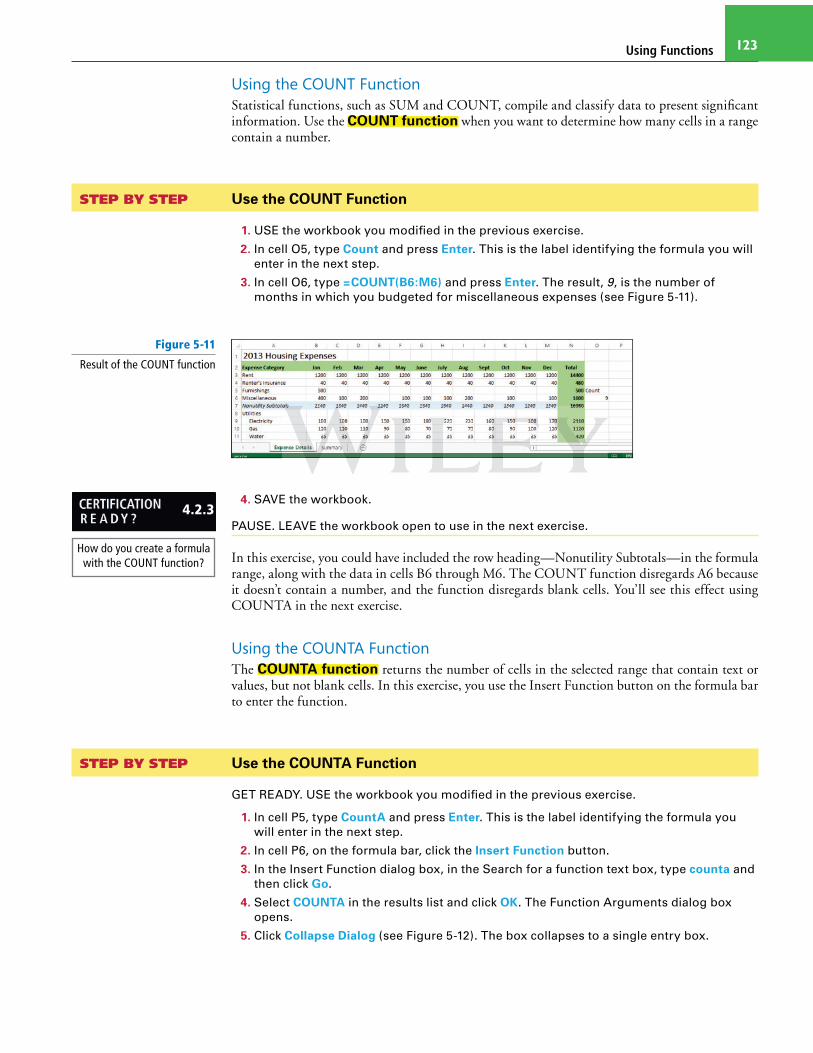
Using the COUNT Function

Statistical functions, such as SUM and COUNT, compile and classify data to present significant information. Use the COUNT function when you want to determine how many cells in a range contain a number.

STEP BY STEP Use the COUNT Function

1. USE the workbook you modified in the previous exercise.

2. In cell O5, type Count and press Enter. This is the label identifying the formula you will

enter in the next step.

3. In cell O6, type =COUNT(B6:M6) and press Enter. The result, 9, is the number of

months in which you budgeted for miscellaneous expenses (see Figure 5-11).

Figure 5-11

Result of the COUNT function



In this exercise, you could have included the row heading—Nonutility Subtotals—in the formula range, along with the data in cells B6 through M6. The COUNT function disregards A6 because it doesn’t contain a number, and the function disregards blank cells. You’ll see this effect using COUNTA in the next exercise.

Using the COUNTA Function

The COUNTA function returns the number of cells in the selected range that contain text or values, but not blank cells. In this exercise, you use the Insert Function button on the formula bar to enter the function.

STEP BY STEP Use the COUNTA Function


1. In cell P5, type CountA and press Enter. This is the label identifying the formula you

will enter in the next step.

2. In cell P6, on the formula bar, click the Insert Function button.

3. In the Insert Function dialog box, in the Search for a function text box, type counta and

then click Go.

4. Select COUNTA in the results list and click OK. The Function Arguments dialog box

opens.

5. Click Collapse Dialog (see Figure 5-12). The box collapses to a single entry box.

How do you create a formula with the COUNT function?

4.2.3

Lesson 5124

Figure 5-12

The Function Arguments dialog box

Collapse Dialog

6. Select A6:M6. The new range appears in the dialog box.

7. Click Expand Dialog shown in Figure 5-13, and click OK to close the dialog box. The

result, 10, is the number of nonblank cells in the range.

Figure 5-13

Expand Dialog Expand Dialog



Using the AVERAGE Function

The AVERAGE function adds a range of cells and then divides by the number of cell entries, determining the mean value of all values in the range. Regarding your personal budget, because the cost of electricity and gas fluctuates seasonally, it might be interesting to know the average monthly amount you might spend over the course of an entire year.

STEP BY STEP Use the AVERAGE Function


1. In cell O8, type Average and press Enter.

2. In cell O9, type =AVERAGE(B9:M9) and press Enter. The result, 175.8333, is your

average expected monthly electricity bill.

3. In cell O10, type =AVERAGE(B10:M10) and press Enter. The result, 93.33333, is your

average expected monthly gas bill (see Figure 5-14).

Figure 5-14

The results of the AVERAGE function

AVERAGE function results

Using Functions 125



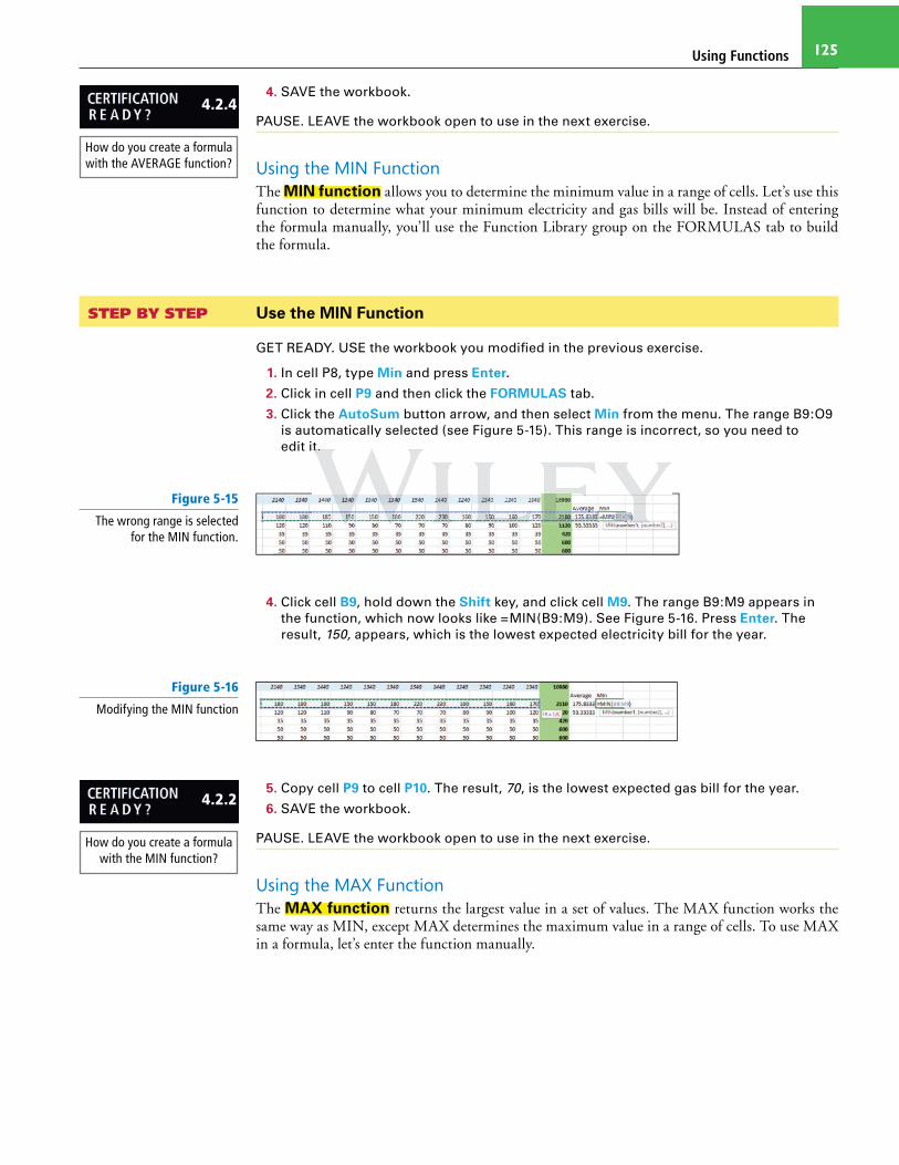
Using the MIN Function

The MIN function allows you to determine the minimum value in a range of cells. Let’s use this function to determine what your minimum electricity and gas bills will be. Instead of entering the formula manually, you’ll use the Function Library group on the FORMULAS tab to build the formula.

STEP BY STEP Use the MIN Function


1. In cell P8, type Min and press Enter.

2. Click in cell P9 and then click the FORMULAS tab.

3. Click the AutoSum button arrow, and then select Min from the menu. The range B9:O9

is automatically selected (see Figure 5-15). This range is incorrect, so you need to

edit it.

Figure 5-15

The wrong range is selected for the MIN function.

4. Click cell B9, hold down the Shift key, and click cell M9. The range B9:M9 appears in

the function, which now looks like =MIN(B9:M9). See Figure 5-16. Press Enter. The

result, 150, appears, which is the lowest expected electricity bill for the year.

Figure 5-16

Modifying the MIN function

5. Copy cell P9 to cell P10. The result, 70, is the lowest expected gas bill for the year.



Using the MAX Function

The MAX function returns the largest value in a set of values. The MAX function works the same way as MIN, except MAX determines the maximum value in a range of cells. To use MAX in a formula, let’s enter the function manually.

How do you create a formula with the AVERAGE function?

4.2.4

How do you create a formula with the MIN function?

4.2.2

itititit. .

Lesson 5126

STEP BY STEP Use the MAX Function


1. In cell Q8, type Max and press Enter.

2. In cell Q9, type =MAX(B9:M9) and press Enter. The result, 230, is the highest monthly

electricity bill that you expect to receive.

3. Copy cell Q9 to Q10. The result, 120, is the highest monthly gas bill that you expect to

receive (see Figure 5-17).

Figure 5-17

The results of the MAX function

MAX function results

4. SAVE the workbook to your Lesson 5 folder and CLOSE it.


USING A FINANCIAL FUNCTION

Functions provide a wide variety of pre-determined calculations for you to choose from, allowing you to easily perform a complex calculation and use it in your worksheet. So far, you have worked with mathematical and statistical functions. Financial functions, in contrast, are designed specif-ically for various finance tasks that you might want to work on.

Use PMT

The PMT function requires a series of inputs regarding interest rate, loan amount (principal), and loan duration, and then calculates the resulting loan payment. In this exercise, you’re interest-ed in purchasing a large flat-panel television, a sound system, and a game box with several games. You calculate the payments you need to make on a two-year loan to purchase the equipment.

STEP BY STEP Use the PMT Function


1. OPEN the 05 Budget PMT data file for this lesson.

2. In cell R2, type Electronics and press Enter.

3. In cell R3, type Interest and press Enter.

4. In cell R4, type Years and press Enter.

5. In cell R5, type Loan Amt and press Enter.

6. In cell R6, type Payment and press Enter.

7. In cell S3, type 7.5% and press Enter. This is the interest rate on the loan.

8. In cell S4, type 2 and press Enter. This is the number of years in which the loan will be

repaid.

9. In cell S5, type 2500 and press Enter. This is the loan amount, which will cover the total

cost of the equipment.

10. In cell S6, type =–PMT(S3/12,S4*12,S5) and press Enter. The result, $112.50, is your

calculated monthly payment (see Figure 5-18).

How do you create a formula with the MAX function?

4.2.2

Bottom Line

ththththe e e wowowoworkbobobobookokok to yoyoyoyour Lesson 5 folder and CLOSE it.

AVAA EEEE E E E Excxcxcelelelel o o o opepepepen n n n to usesese in thththe next exexexexercrcrcisise.e.e.

Using Functions 127

Figure 5-18

The result of the PMT function

11. SAVE the workbook to your Lesson 5 folder as 05 Budget PMT Solution and CLOSE it.


The PMT function calculates a loan payment and uses the syntax =PMT(rate, nper, pv, [fv], [type]). The three required arguments for the PMT function are:

• Rate: The interest rate charged per period (for example, per month)

• Nper: The total number of payments for the loan

• Pv: The present value of the loan—in other words, how much you owe; also known as the principal

Optional arguments include the future value (fv), which is a cash balance you want to attain after the last payment is made, and type, which indicates when payments are due using the number 1 (due at the beginning of a period) or 0 (due at the end of a period).

When functions take more than one argument, you enter them in a single set of parentheses, separated by commas.

For the purposes of your budget, you include the negative sign (–) at the beginning of the PMT function (=–PMT(S3/12, S4*12,S5)) because the function calculates a payment as a negative value by default. By including the negative sign, the payment appears as a positive number. This follows a basic rule of mathematics: The negative of a negative is a positive.

You divide the first set of values by 12 because 7.5% is the annual interest rate, and dividing it by 12 gives you the monthly interest rate. You multiply the second set of values by 12 to convert the loan term from years to months.

USING FORMULAS TO CREATE SUBTOTALS

Many Excel veterans use formulas to create subtotals. Subtotaling lets you more easily analyze large sets of data. You can specify ranges for subtotals even if the ranges are not contiguous. In this section, you learn how to use the SUBTOTAL function applied to cell ranges and named ranges.

Selecting and Creating Ranges for Subtotaling

You learn how to select ranges and name them in Lesson 4. You use those skills in this section to prepare to subtotal parts of your budget worksheet.

STEP BY STEP Select and Create Ranges for Subtotaling


1. OPEN the 05 Budget Subtotals data file for this lesson.

2. Select B7:M7.

3. On the FORMULAS tab, in the Defined Names group, click the Define Name button. The

New Name dialog box opens.

Bottom Line

a a argrgrgrgumumumenenenentsts i inclululudededede t t thehehehe f f f futururure vavavavalue (fv)v)v)v), whwhwhicicich h h h is a a a a casasasash babababalalalaaymememementntnt i i i is s s s mamamamadededede, , , and d d tytytype, whwhwhich indicacacacatetetes s whwhwhwhen payayayaymememementntnts ar

the bebebebegigigiginnnnnnnninining g g g ofofofof a perioioiod)d)d) or 0 (due at ththththe end ofofof a perioioiod)d)d).

Lesson 5128

4. In the Name text box, verify that Nonutility_Subtotals appears (see Figure 5-19). Click

OK. This names a range for the nonutility subtotal figures.

Figure 5-19

The New Name dialog box

5. SAVE the workbook to your lesson 5 folder as 05 Budget Subtotals Solution.


Building Formulas for Subtotaling

You can calculate subtotals using the SUBTOTAL function, which returns a subtotal for a list. This function recognizes values, cell references, ranges, and named ranges, and totals values cre-ated using SUM, AVERAGE, COUNT, and many other functions. This exercise shows you how to use the SUBTOTAL function to sum ranges of cells, both named and unnamed.

STEP BY STEP Build Formulas to Subtotal


This lesson shows you how to build subtotals using the SUBTOTAL function. Lesson 9 , “Work-ing with Data and Macros,” covers grouping and outlining to produce subtotals.

1. In cell B17, type =SUBTOTAL(9,B7,B16), as shown in Figure 5-20. Press Enter. This

formula adds the nonutility subtotal and utility subtotal for January.

Figure 5-20

Entering the SUBTOTAL formula to add two cells that

include SUM functions

SUBTOTAL formula

Cell B7

Cell B16

2. Copy cell B17 to C17:M17. All monthly subtotals are entered.

3. In cell N17, type =SUBTOTAL(9,B7:M7,B16:M16), as shown in Figure 5-21. Press Enter.

This formula adds all nonutility and utility expenses for the year.

Figure 5-21

Entering the SUBTOTAL function to add two cell ranges

Cross Ref

UMUMUMUM, AVERERERERAGE,E,E,E, C C COUNT, and many other functions. ThisUBUBUBUBTOTOTOTATATATAL L L L funcncncnctititition to o o o sum m m rararanges of f f cecececelllllls, b b bototototh h nanananamemememed anananand d d

Using Functions 129



The SUBTOTAL function uses the syntax =SUBTOTAL( function_num,ref1,[ref2],...).

As you enter the SUBTOTAL function, Excel, displays a list of the function numbers for the first argument. The function number for SUM is 9. You can learn the function numbers for other functions, such as AVERAGE, COUNT, and COUNTA, when entering the SUBTOTAL func-tion or by searching for SUBTOTAL in Excel Help.

Ref1 is the first cell reference, cell range, or named range you want to subtotal. You can include additional cells or ranges by separating them with commas.

In the exercise, you also used the SUBTOTAL function to calculate the total for the budget in cell N17. Creating a total is a standard bookkeeping technique, and allows you to track and adjust subtotals while keeping the final total current.

Modifying Ranges for Subtotaling

Once you create a range in a subtotal, you can easily modify it by editing the range in the formula. You can also modify ranges that are already used in formulas that include the SUBTOTAL function.

STEP BY STEP Modify Ranges for Subtotaling


1. In cell N17, notice that the result of the current formulas is 24,230.

2. Use the formula bar to modify the formula in N17 like this: =SUBTOTAL(9,Nonutility_

Subtotals,Utility_Subtotals). See Figure 5-22. Press Enter. This formula replaces the

cell ranges with named ranges to add all nonutility and utility expenses for the year,

and the result remains the same at 24,230.

Figure 5-22

Modifying the SUBTOTAL function to

use named ranges

Modifying the formula

3. Click in cell B19 and then click in the formula bar. Change the formula from

=SUM(Q1Expenses) to =SUBTOTAL(9,Q1Expenses). This cell sums the named range

Q1Expenses. Because the named range includes monthly data and subtotals, you need

to correct the range to include only subtotal figures.

4. On the FORMULAS tab, in the Defined Names group, click Name Manager.

5. Select Q1Expenses in the list and click Edit. The Edit Name dialog box opens (see

Figure 5-23).

alalalalsososo m m modififify y y rarararangeseses t t thahahahat are already used in formulas that include

Rananangegegeges fofofofor r r Subtbtbtbtotototalininininggg

Lesson 5130

Figure 5-23

The Edit Name dialog box

6. Highlight everything in the Refers to text box and press Backspace to delete it.

7. Click cell B7, press and hold the Shift key, and click D7. The range B7:D7 is highlighted.

8. Press and hold the Ctrl key while clicking cells B16, C16, and D16. The selections are

shown in Figure 5-24.

Figure 5-24

Selecting multiple ranges to include in the Q1Expenses

named range

Cells B7:D7

Cells B16:D16

Formula being modifi ed

9. In the Edit Name dialog box, click OK.

10. In the Name Manager dialog box, click Close.

11. To verify that you selected the proper ranges for the Q1Expenses range, open the

Name box drop-down list (to the left of the formula bar) and select Q1Expenses. The

ranges B7:D7 and B16:D16 are selected (see Figure 5-25).

Figure 5-25

Verifying the new ranges for Q1Expenses

Cells B7:D7 are selected.

Cells B16:D16 are selected.

12. Create named ranges for Q2Expenses (E7:G7, E16:G16), Q3Expenses (H7:J7, H16:J16),

and Q4Expenses (K7:M7, K16:M16).

13. Copy the formula from cell B19 to B20:B22. Edit the formulas in cells B20, B21, and B22

to use the appropriate named range. For example, the formula in cell B20 should be

=SUBTOTAL(9,Q2Expenses).

14. SAVE the workbook to your Lesson 5 folder and CLOSE it.


UNCOVERING FORMULA ERRORS

Formulas, because of the sometimes-complex mathematics behind them, are prone to errors when you enter them manually. Fortunately, Excel provides easy-to-use tools to fi nd and correct prob-lems. In this exercise, you intentionally create an error, and then learn how to correct that error.

Bottom Line

Cells B16:D16

dit NaNaNaNamememe diaiaiaialolololog bobox,x,x,x, c c clickckckck OKOKOK.

Using Functions 131

Reviewing Error Messages

The best way to resolve an error is to analyze, or audit, the error message Excel provides for you. A warning icon appears to the left of cell errors, and clicking that icon provides a pop-up menu with formula evaluation and formula editing commands, and access to Excel Help.

STEP BY STEP Review an Error Message


1. OPEN the 05 Budget Error data file for this lesson.

2. Click in cell S6.

3. Edit the formula to change S3 to R3 and press Enter. The first cell reference in the PMT

formula now points to the wrong cell. A #VALUE! error displays in cell S6 (see Figure

5-26).

Figure 5-26

An error displays in cell S6.

4. Click in cell S6. Click the small, yellow warning icon to the left of the cell. A pop-up

menu appears (see Figure 5-27). The first item tells you that there is a value error in the

function.

Figure 5-27

The pop-up menu for the error

5. In the menu, select Help on this error. Excel Help opens to a page on information

regarding formula errors. Browse the help topics to see if any of the potential solutions

apply to your situation.

6. CLOSE the Excel Help window.

7. SAVE the workbook to your Lesson 5 folder as 05 Budget Error Solution.


Notice the small green triangle in the upper-left corner of cell S6. This means the cell contains a formula error.

To evaluate the error in the formula, select the Show Calculation Steps option from the pop-up menu that appears after you click the warning icon. The Evaluate Formula dialog box, shown in Figure 5-28, indicates the first part of the function is incorrect. In this case, the reference to cell R3 points to a cell containing text. The cell reference should be S3, which contains the interest figure.

Lesson 5132

Figure 5-28

The Evaluate Formula dialog box

Once you know how to correct an error, you can click the warning icon and select Edit in Formula Bar from the pop-up menu. Make the necessary corrections directly in the formula.

Tracing and Removing Trace Arrows

It’s not always easy to resolve a formula error, even using the Show Calculation Steps command, the Evaluate Formula dialog box, and Excel Help. Another method is to use trace arrows, which show the relationship between formulas and the cells they refer to.

STEP BY STEP Trace a Formula and Remove Trace Arrows


1. Select cell S6 if it’s not already selected.

2. On the FORMULAS tab, in the Formula Auditing group, click Trace Precedents. Two

arrows appear (see Figure 5-29). One arrow extends from cell R3 to cell S6, and

another (combined) arrow extends from cells S4 and S5 to S6. The arrows indicate that

the formula in cell S6 refers to cells R3, S4, and S5, referred to as precedent cells.

Figure 5-29

The worksheet showing trace precedents

3. On the FORMULAS tab, in the Formula Auditing group, click Remove Arrows. The trace

arrows disappear from the worksheet.

4. Click cell S4. On the FORMULAS tab, in the Formula Auditing group, click Trace

Dependents. One arrow appears from cell S4 to cell S6 (see Figure 5-30). The arrow

indicates that cell S4 is part of the formula in cell S6.

Figure 5-30

The worksheet showing trace dependents

5. SAVE the workbook and CLOSE it.


ormumumumulalalala a a andndndnd R R R Remememovovove TrTrTracace Arrorororowswswsws

Y. USESESESE t t the w w w wororororkbook k k yoyoyou momomodididifiefiefied d d ininin thehehe p p prerererevivivivious exexexexererercise

Using Functions 133

You can use trace precedents and trace dependents for formulas that reference cells in another workbook. However, the external workbook must be open before you use the trace commands.

DISPLAYING AND PRINTING FORMULAS

When you audit the formulas in a worksheet, you might find it useful to print the worksheet with the formulas displayed. In this exercise, you display formulas for printing.

STEP BY STEP Print Formulas


1. OPEN 05 Budget Print from your Lesson 5 folder.

2. On the FORMULAS tab, in the Formula Auditing group, click Show Formulas. The

formulas appear in the worksheet (see Figure 5-31).

Figure 5-31

Formulas displayed in the worksheet

3. Click the FILE tab. Click Print and view the Print Preview.

4. Click the Portrait Orientation button and select Landscape Orientation.

5. At the bottom of the print settings, click the Page Setup link to open the Page Setup

dialog box.

6. On the Page tab of the dialog box, click Fit to: and leave the defaults as 1 page(s) wide

by 1 tall (see Figure 5-32). Click OK to close the dialog box.

Figure 5-32

Settings in the Page Setup dialog box

Bottom Line

Another WayYou can also dis-

play formulas in the worksheet by pressing Ctrl + ` (the grave accent mark). The grave accent mark is usually located on a key on the upper-left part of the keyboard.

Lesson 5134

7. At the top-left corner of the Backstage view window, click the Print button to print the

worksheet with formulas displayed.

You learn more about print options in Lesson 7 , “Formatting Worksheets.”

8. On the FORMULAS tab, in the Formula Auditing group, click Show Formulas again to

stop displaying formulas in the worksheet.

9. SAVE the workbook to your Lesson 5 folder as 05 Budget Print Solution and CLOSE it.

CLOSE Excel.

SKILL SUMMARY

In this lesson you learned how: Exam ObjectiveObjective Number

To find tools for building functions on

the FORMULAS tab.

To display dates and times with

functions.

To use the SUM function. Demonstrate how to apply the SUM

function.

4.2.1

To use the COUNT function. Demonstrate how to apply the COUNT

function.

4.2.3

To use the AVERAGE function. Demonstrate how to apply the AVERAGE

function.

4.2.4

To use the MIN and MAX functions. Demonstrate how to apply the MIN and

MAX functions.

4.2.2

To use the PMT financial function.

To use formulas to create subtotals.

To respond to formula errors.

To display and print formulas.

Knowledge Assessment

Multiple Choice

Select the best response for the following statements.

1. Which of the following calculates the total from the adjacent cell through the first

nonnumeric cell by default, using the SUM function in its formula?

a. AVERAGE

b. AutoSum

c. COUNTA

d. MAX

2. The arguments of a function are contained within which of the following?

a. brackets

b. asterisks

c. commas

d. parentheses

Cross Ref

pply

fufufufunction.

COUOUOUNTNTNTNT f f f funununctctctctioioioion.n.n. DeDeDemonstratatatate e e hohohohow w w w to apppppppplylyly t t t thehehehe COU

fufufunctionononon.

Using Functions 135

3. When using the SUBTOTAL function, which is the function number for the SUM

function?

a. 1

b. 4

c. 9

d. 11

4. You want to add a range of cells and then divide by the number of cell entries,

determining the mean value of all values in the range. Which function do you use?

a. SUBTOTAL

b. AVERAGE

c. COUNT

d. PMT

5. Which of the following is not a required argument for the PMT function?

a. Fv

b. Rate

c. Nper

d. Pv

6. You want to calculate the number of nonblank cells in your worksheet. Which function

do you use?

a. SUM

b. COUNT

c. COUNTA

d. MAX

7. You want to create a formula that calculates the number of years you have lived. You

were born in 1991. Which of the following formulas is correct?

a. =YEAR(TODAY())-1991

b. =YEAR(TODAY())+1991

c. =YEAR(COUNT())-1991

d. =YEAR(COUNT())+1991

8. Which of the following statements accurately describes the default selection for

AutoSum?

a. You must make the selection before clicking AutoSum.

b. By default, AutoSum totals all entries above the cell in which the formula is located,

even if the cells contain a mix of numeric and nonnumeric content.

c. By default, AutoSum calculates the total from the adjacent cell through the first

nonnumeric cell.

d. AutoSum does not have a default selection.

9. You want to sum multiple noncontiguous cell ranges that are named. Which of the

following is best to use?

a. AutoSum

b. SUBTOTAL

c. MAX

d. MIN

10. The COUNT and MIN functions are examples of which category of functions?

a. text

b. statistical

c. financial

d. logical

True / False

Circle T if the statement is true or F if the statement is false.

T F 1. All functions require arguments within parentheses.

T F 2. Using functions helps to ensure the accuracy of a formula’s results.

T F 3. The TODAY function returns the current date in a worksheet.

T F 4. The AVERAGE function returns the number of cells in the selected range that

contain text or values, but not blank cells.

T F 5. When functions take more than one argument, you should enter them in

multiple sets of nested parentheses, separated by commas.

MAMAMAMAXXX

wawantntnt t t to crcrcrcreaeaeaeatetete a a a a formumumula thahahat t calculatatatateses thehehe numbebebeber r r r ofofof y y yea

bororororn inininin 19999991.1.1.1. W W Whichchch o o of the e e fofollowing g g g fofoformulululas is cococorrrrrrect?

=YEAR(R(R(R(TOTOTOTODADADADAY(Y(Y(Y())))))-199111

=YEAR(R(R(TOTOTODAY(Y(Y(Y())+1991

Lesson 5136

T F 6. In the PMT function, the Nper argument is the total number of payments for the

loan.

T F 7. You can use a range in the SUBTOTAL function, but you cannot modify the

range once it’s in use.

T F 8. A cell cannot be a trace dependent and a trace precedent for the same formula.

T F 9. You can refer to the TODAY and NOW functions in other formulas to perform

calculations.

T F 10. To evaluate the error in the formula, select the Edit in Formula Bar option from

the pop-up menu that appears after you click the warning icon.

Competency Assessment

Project 5-1: Use Statistical Functions to Analyze Game Wins and Losses

You work for Wingtip Toys and have been playing three new games each day to master them, hoping to demo the games in the retail store. You’ve been keeping track of your wins and losses in a worksheet. A “1” indicates a win, and a “0” indicates a loss.


1. OPEN the 05 Game Stats data file for this lesson.

2. In cell E3, type =AVERAGE(B3:D3) and press Enter.

3. Copy the formula in E3 to E4:E12.

4. Click cell G2.

5. On the FORMULAS tab, in the Function Library group, click the AutoSum button arrow

and select Count Numbers.

6. Click cell B3 and drag the mouse pointer to cell D12.

7. Release the mouse and press Enter to accept the range B3:D12. The result, 30, is the

total number of times you played the games in 10 days.

8. In cell G3, type =SUM(B3:D12) and press Enter. The result, 17, represents the total

number of times you won the games.

9. In cell G4, type =G2-G3 and press Enter. The result, 13, represents the total number of

times you lost the games.

10. On the FORMULAS tab, in the Formula Auditing group, click Show Formulas. The

formulas appear in the worksheet.

11. Click the Show Formulas button again to turn off the display of formulas.

12. SAVE the workbook to your Lesson 5 folder as 05 Game Stats Solution and then CLOSE

the file.

LEAVE Excel open to use in the next project.

Project 5-2: Create Formulas to Calculate Totals and Averages

An employee at Wingtip Toys has entered second quarter sales data into a worksheet. You will enter formulas to calculate monthly and quarterly totals and average sales.


1. OPEN 05 Wingtip Toys Sales from the data files for this lesson.

2. Click cell B11, type =SUM(B4:B10), and press Enter.

Y. LLLLAAAAUNUNUNCCCCHHH E E Excxcxcelelelel if ititit is s s not t t alalalready rurururunnnnining.

the 050505 G G Gamamame e e StStStatatats datatata a a file fofor this lesesesessoson.s

E3, typepepepe =AVEVEVERAGEGEGE(B(B(B3:3:3:D3D3D3))) a a andndnd p p prereressssss EnEnEnteteterrr..

Using Functions 137

3. Click cell C11. On the FORMULAS tab, in the Function Library group, click Insert

Function.

4. In the Insert Function dialog box, select SUM and click OK.

5. In the Function Arguments dialog box, click Collapse Dialog and select C4:C10, if it’s

not already entered.

6. Click the Expand Dialog button and click OK to close the dialog box.

7. Copy the formula from C11 to D11.

8. Click cell E4. On the FORMULAS tab, in the Function Library group, click the AutoSum

button. Press Enter to accept B4:D4 as the cells to total.

9. Click cell E5 and then in the Function Library group click Insert Function. In the Insert

Function dialog box, SUM will be the default. Click OK.

10. The range B5:D5 should appear in the Number1 box in the Function Arguments dialog

box. Click OK to close the dialog box.

11. Click cell E5 and use the fill handle to copy the formula to E6:E10.

12. Click cell E11. In the Function Library group click AutoSum. Press Enter to accept the

range as E4:E10.

13. Click cell F4. Click the Insert Function button. Select AVERAGE in the Insert Function

dialog box and click OK. In the Function Arguments dialog box, click OK.

14. Click in the formula bar and change E4 to D4. Click OK.

15. Click cell F4 and use the fill handle to copy the formula to F5:F11.

16. SAVE the workbook to your Lesson 5 folder as 05 Wingtip Toys Sales Solution and then

CLOSE the file.

LEAVE Excel open to use in the next project.

Proficiency Assessment

Project 5-3: Compare Payments

Monica recently graduated from college and needs to replace her current vehicle. She wants to use Excel 2013 to help her decide whether she should buy a lower priced vehicle or something newer.


1. OPEN 05 Compare Payments from the data files for this lesson.

2. Enter a formula that displays today’s date in cell B2.

3. Enter a formula in cell B4 that calculates a monthly interest rate based on the rate

displayed in B3. Be sure to use an absolute cell reference to B3.

4. Use the PMT function to calculate loan payments for each dollar amount below the

Amount Borrowed heading. Be sure to use absolute cell references for the rate and

nper arguments, and add a minus sign before PMT in the formula so the result is a

positive value.

5. SAVE the workbook to your Lesson 5 folder as 05 Compare Payments Solution and

then CLOSE the file.

LEAVE Excel open for the next project.

cecececellllllll F4 andndndnd usesese t thehehe fill handle to copy the formula to F5:F

E ththththe e e wowoworkrkrkrkbobobookokok t t t to yoyoyoururur Lesesessososon 5 foldldlderererer as 0 0 05 5 5 WiWiWingngngtititip ToToToys

OSE ththththe e e e filfilfilfile.e.e.e.

Excel opopopopen to o o ususususe in t t thehehehe nexexexext t t prprprojojojececect.t.t.

Lesson 5138

Project 5-4: Resolve Formula Errors

You work for the School of Fine Arts and have been asked to correct errors in a student GPA worksheet.


1. OPEN 05 Fine Art Formulas from the data files for this lesson.

2. An error occurs in cell F4. Examine the formula in the formula bar and correct the error

manually.

3. For the error in cell F6, click the warning icon and use one of the options in the pop-up

list to correct the error.

4. For the error in cell F12, use the Show Calculation Steps command to determine the

source of the error and then correct the error using the formula bar.

5. One of the formulas at the bottom of the worksheet needs to be corrected. Use trace

arrows to determine which formula’s range includes an extra cell and correct the

formula.

6. SAVE the workbook to your Lesson 5 folder as 05 Fine Art Formulas Solution and then

CLOSE the file.


Mastery Assessment

Project 5-5: Build Formulas to Track Merchandise Stock Levels

Wide World Importers sells a variety of fine wool rugs, textiles, ceramics, furniture, and statues from the Middle East. The company tracks levels of stock in nine different categories, and keeps several units of each type of stock in five warehouses spread across the region. You have been asked to track all 45 stock levels.


1. OPEN 05 Importers Stock from the data files for this lesson.

2. Use the SUM formula to total the number of stock units in each warehouse.

3. Calculate the number of stock units that are at zero (0) across all six warehouses in cell

B14.

4. Calculate the maximum number of stock units in any warehouse in cell B15.

5. Calculate the minimum number of stock units in any warehouse in cell B16.

6. SAVE the workbook to your Lesson 5 folder as 05 Importers Stock Solution and then

CLOSE the file.


Using Functions 139

Project 5-6: Complete the Analysis Sheet in the Budget Workbook

Blue Yonder Airlines wants to analyze the sales and expense data from its four-year history. You will complete the Analysis sheet to summarize the data.


1. OPEN 05 Income Analysis Start from the data files for this lesson.

2. On the Analysis sheet, calculate average sales for each of the four service categories

using range names. Use Name Manager to examine range names in the workbook

before you enter the formulas.

3. Calculate the average expenses for each of the four service categories.

4. Calculate the maximum sales for each of the four service categories.

5. Calculate the maximum expenses for each of the four service categories.

6. SAVE the workbook to your Lesson 5 folder as 05 Income Analysis Solution and then

CLOSE the file.

CLOSE Excel.

Circling Back 1140

Circling Back 1

The Graphic Design Institute offers associate’s and bachelor’s degrees in graphic design, with a full slate of in-classroom and online classes. Students from the United States and several other coun-tries attend the Institute as full-time students during fall and spring semesters, or by participating in accelerated programs offered twice a year.

As an employee in the organization’s home office, you create workbooks related to the Institute’s programs and fundraising efforts.

Project 1: Creating a Workbook and Entering Data

Your first task is to create a workbook that can serve as the initial structure for recording students’ GPAs. The student names you type in the worksheet are in an accelerated program and work with a specific instructor.


1. Open a new, blank workbook.

2. In cell A1, type Graphic Design Institute and press Enter.

3. In cell A2, type Instructor: Sachin Karnik and press Enter.

4. In cells A3:F3, type the following:

Name

ID

GD1

DM1

Type1

GPA

5. In cells A4:A14, type the following:

Con, Aaron

Cunha, Goncalo

Byham, Richard A.

Klimov, Sergey

Chopra, Manish

Davison, Eric

Hensien, Kari

Levitan, Michal

Paschke, Dorena

Wang, Tony

Ribaute, Delphine

6. Double-click the right border of column A to expand the column width.

7. In cell B4, type 13001.

8. Copy cell B4 to B5. In cell in B5, change 13001 to 13002.

9. Highlight cells B4:B5, point to the fill handle in the lower-right corner of cell B5, drag it

to cell B14, and release the mouse.

10. Click the FILE tab to open Backstage view. In the left pane, click Save As to display the

save options.

11. Under Save As, click Computer, and then click Browse.

12. Use the left navigation pane in the Save As dialog box to navigate to your student data

folder.

n n newewewew, blanananank workrkrkrkbobobobook.

A1A1, , , , tytytype G G Grararaphicicic D D Desesesigigign n n Instststitititute and d d prprpresesess s s EnEnEnteteterrr.

A2, tytytytypepepe InInInstststruruructctctor: SaSachin Kararnik and d d d prprpresesess s s s Enteteterrr....

A3:F3F3F3F3, , , typepepepe thehehe follololowiwiwing:

Circling Back 1 141

13. In the toolbar near the top of the Save As dialog box, click New folder. A folder icon

appears with the words New folder selected.

14. Type Circling Back and press Enter.

15. Double-click the Circling Back folder.

16. In the File Name box, type GPA Solution.

17. Click the Save button.

18. CLOSE the file.


Project 2: Using Basic Formulas and Functions

The Graphic Design Institute is supported in part by individual and corporate tax-deductible con-tributions. Contributors are asked to select a fund to which their contribution applies. It is your responsibility to create some simple statistics to help senior management understand the number of contributors, the average amount contributed per organization and per individual, and the minimum and maximum dollar amounts of all contributions.


1. Open Contributions from the student data files.

2. In cell A33, type Total Contributions and press Enter.

3. In cell C33, type =SUM(C4:C32) and press Enter.

4. Select cells C4:C32. On the FORMULAS tab, in the Defined Names group, click the

Define Name button arrow and select Define Name.

5. In the New Name dialog box, accept the defaults and click OK. A range named Amount

is created.

6. In cell B35, type =COUNT(C4:C32) and press Enter. The result represents the number

of contributions made to Graphic Design Institute.

7. Click in B36. On the FORMULAS tab, in the Function Library group, click Insert

Function. In the Insert Function dialog box, search for AVERAGE, select it in the Select

a function list box, and click OK.

8. In the Function Arguments dialog box, click Collapse Dialog and select C4:C21.

9. Click the Expand Dialog button and click OK to close the dialog box. A triangle appears

in the upper left corner of B36 and an error message button is displayed. Click the

button arrow, and then click Ignore Error. The result in B36 represents the average

dollar amount contributed by organizations.

10. Copy the formula in cell B36 to B37.

11. With B37 selected, change the range in the formula to C22:C32. A triangle appears in

the upper left corner of B37 and an error message button is displayed. Click the button

arrow, and then click Ignore Error. The result in B37 represents the average dollar

amount contributed by individuals.

12. In cell B38, type =MIN(Amount) and press Enter. This formula uses the named range

and displays the minimum dollar amount contributed by an organization or individual.

13. In cell B39, type =MAX(Amount) and press Enter. This formula displays the maximum

dollar amount contributed by an organization or individual.

14. SAVE the workbook to your Lesson 5 folder as Contributions Solution in the Circling

Back folder.

LEAVE the workbook open for the next project.

enenenen CoCoContribububutions s s frfrfrfromomom the student data files.

ell A3A3A3A33, typypypype e e e Totatatal CoCoContntntribububutiononons and prprprpresesess s s EnEnEnteteterrr.

ell C3C3C33,3,3,3, t t typypype e e e =S=S=SUMUMUM(C(C4:4:C32)2)2) a and pressssssss EnEnEnteteterrr.

ct celelelellslsls C4:C:C:C323232. On t t thehehe FORORORMMULALALAS S S S tatatatab,b, in ththe e e e Definfinfinededed Nam

fine NaNamememe butttttttton arrow andndndnd selelelect t t DeDeDefinfinfine NaNaName

Circling Back 1142

Project 3: Configuring a Workbook for Printing

You have prepared a workbook with data related to contributions to the Institute and have been asked to print copies for a meeting to be attended by senior management.

GET READY. USE the workbook you saved in the previous project.

1. Select cells A1:C39.

2. Click the PAGE LAYOUT tab, and in the Page Setup group, click the Print Area button

and select Set Print Area.

3. Click the FILE tab to access Backstage view.

4. Click Print and view the document in the Print Preview pane.

5. Click the Scaling button arrow, and then click Custom Scaling Options.

6. In the Page Setup dialog box, in the Adjust to box, type 110. This action makes the text

a little larger without having to change the font in the document. Click OK.

7. Click Print.

8. Click anywhere in the worksheet to remove highlighting from the selection.

9. Check the Quick Access Toolbar. If you do not see the Quick Print button, click the

Customize Quick Access Toolbar arrow at the end of the toolbar and select Quick Print.

The Quick Print button appears on the toolbar, which you can use to print any Excel

document in the future.

10. SAVE the workbook to your Lesson 5 folder as Contributions Print Solution in the

Circling Back folder, and then CLOSE the file.

CLOSE Excel.

hehehe w w worororkbkbkbkbooooooook to y y y youour r r r LeLeLeLessonononon 5 5 5 5 folder asasas CoCoContntntririribububutititiononons PrPrPrininin

Bacacacack k k fofofofoldldldlderererer, , , anananand d d thenenen CLOLOLOSESE the file.e.e.e.

el.

moac excel 2013 exam 77 420 - cabarrus county schools · table 5-1 lists common excel functions,...

Documents