MOBIUS BEATS: THE TWISTED SPACES OF SLIDING WINDOW AUDIONOVELTY FUNCTIONS WITH RHYTHMIC SUBDIVISIONS

Christopher J. TralieDuke University

Department of Mathematics

John HarerDuke University

Department of Mathematics

ABSTRACT

In this work, we show that the sliding window embed-dings of certain audio novelty functions (ANFs) represent-ing songs with rhythmic subdivisions concentrate on theboundary of non-orientable surfaces such as the Mobiusstrip. This insight provides a radically different shape-based, topological approach to classifying types of rhythmhierarchies. In particular, we use tools from topologicaldata analysis (TDA) to detect the presence and type ofrhythmic subdivisions, and we use thresholds derived fromTDA to build graphs at different scales. The Laplacianeigenvectors of these graphs contain information whichcan be used to estimate tempos of the subdivisions. Weshow a proof of concept example on audio from theMIREX tempo training dataset, and we hope in futurework to use these descriptors in classification pipelines.

1. SLIDING WINDOW EMBEDDINGS OF PULSES

Given M lags and an interval τ , the sliding window em-bedding of a 1D function f(t) 1 is the space curve is pa-rameterized as

SM,τ [f ](t) =

f(t)

f(t+ τ)...

f(t+Mτ)

∈ RM+1 (1)

Under the right conditions, sliding window embeddingsof time series which witness deterministic processes canbe used to reconstruct the state spaces of those processes[5]. A simple example is a pure sinusoid, for whichSM,τ [cos](t) = u cos(t) + v sin(t) for two fixed vectorsu,v ∈ RM+1 (see [4]), which is an equation parameter-izing an ellipse. More generally, as shown by the authorsof [4], the sliding window embedding of any periodic func-tion (i.e. f(t) = f(t + T ) for some T ∈ R+) lies on a

1 For ease of exposition, we define the sliding window as acting oncontinuous 1D functions, but in practice these functions are discretized toN samples, and interpolation may be necessary for some M, τ choices.

c© Christopher J. Tralie, John Harer. Licensed under a Cre-ative Commons Attribution 4.0 International License (CC BY 4.0). Attri-bution: Christopher J. Tralie, John Harer. “Mobius Beats: The TwistedSpaces of Sliding Window Audio Novelty Functions with Rhythmic Sub-divisions”, Extended abstracts for the Late-Breaking Demo Session of the18th International Society for Music Information Retrieval Conference,Suzhou, China, 2017. Authors supported by NSF DKA-1447491.

Figure 1. Self-similarity matrices (SSMs) of sliding win-dow embeddings of various harmonic pulse trains.

0 π

2π, 0π

d

t

t+π 2π, 0 4π/3

2π/3d d

d

Figure 2. (Left) The Mobius strip (2 on 1) with itsboundary drawn in blue and arrows showing identifications(glued locations). In this rendering, the boundary jumpsfrom the lower right corner to the upper right corner ofthis diagram because of the twist. A uniform Mobius striphas the property that for its boundary [0, 2π] → X(t),||X(t)−X(t+π)||2 is a constant d (the width of the strip).(Right) Analogous structure for the 3 on 1 geometry.

topological loop, though the geometry may be quite com-plicated. For instance, the sliding window embedding ofa cos(t) + b cos(2t) lies on the boundary of a Mobius stripif b > a [4] (note that the boundary of a Mobius strip is asingle loop, see Figure 2). Inspired by this result, we inves-tigate the sliding window embeddings of “k on 1 harmonicpulse trains” as a model for ANFs with subdivision; that is

f(t) = aδ(t(modT )) + bδ(kt(modT )) (2)

for some constants a, b and some positive integer k,where δ is the Kronecker delta. Given Mτ = 2T , weobserve that the pairwise distances between windows are

d(s, t) =

0 |s− t| = lT

2|b− a| |s− t| = l′T + T/k∞ otherwise

(3)

for l, l′ ∈ Z. That is, the windows line up perfectly afteran integer number of periods, but they also line up locallyat every subdivided beat shift. Otherwise, they don’t lineup at all, though in practice we smooth the pulses so adja-cent windows in time have a finite distance. Figure 1 showsSSMs for smoothed pulses for different cases. For k = 2,

m

gr

Figure 3. Sliding window of the 2 on 1 pulse train, T =200, k = 2, a = b = 1, Mτ = 2T , and the first window ishighlighted in red on the left plot. The horizontal red lineindicates the distance between adjacent windows in time,and the green line indicates the local min distance at T/2.Persistence diagrams for fields Z2,Z3,Z5 are on the right.

Figure 4. Sliding window embedding of the audio noveltyfunction (ANF) from part of Erykah Badu’s “Green Eyes,”which has a 3 on 1 structure, as indicated by the Z3 change.

this matches the geometry of the Mobius strip boundary,which is locally close to itself at a lag of T/2 (Figure 2).

1.1 Discovering Subdivisions with TDA

To discover these shapes in data, we use techniques fromtopological data analysis (TDA). In broad strokes 2 , TDAprovides a way to quantify “cycles” (connected compo-nents, loops, voids) at different scales in point cloud data.It uses a computable invariant known as homology, whichturns the problem of quantifying these features into a linearalgebra problem. For certain shapes with “torsion,” such asthe Mobius strip, the field of coefficients used in the vectorspace representing the objects can change the homology.In the case of the Mobius strip boundary, if we use Z2 (bi-nary) coefficients, a loop class is “born” (i.e. forms for thefirst time) at a scale 3 r equal to the distance between ad-jacent windows (red line, Figure 3) and “dies” (i.e. fills in)at a scale slightly larger than the strip width g (green line).These changes are summarized in a “persistence diagram”which has a dot for every class, with its birth time on thex-axis and death time on the y-axis. At a scale equal tothe strip width g, another class is born, which dies at themaximum distance m. By contrast, for all other field co-efficients, there is only one significant class which is bornat r and dies at m (see [4] for a similar example with puresinusoids). In general, for finite fields with p elements,where p is a prime factor of k, this “splitting” of one class[r,m] into [r, g] and [g,m] will occur, which can be usedto identify subdivision. Figure 4 shows a 3 on 1 examplefrom a real audio novelty function.

2 This is an intricate subject, details are beyond our scope; see [2]3 By scale x, we mean a “Rips complex” built from distance infor-

mation between windows. This is a combinatorial object with a vertexfor each window, edges between windows that are at most x apart, andtriangles between triples of windows which are pairwise at most x apart.

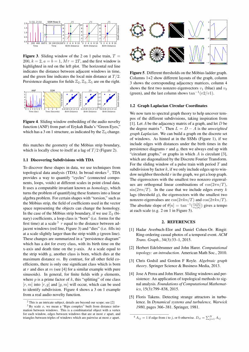
Figure 5. Different thresholds on the Mobius ladder graph.Columns 1+2 show different layouts of the graph, column3 shows the corresponding adjacency matrices, column 4shows the first two nonzero eigenvectors v1 (blue) and v2(green), and the last column shows tan−1(v2/v1).

1.2 Graph Laplacian Circular Coordinates

We now turn to spectral graph theory to help uncover tem-pos of the different subdivisions, taking inspiration from[1]. Let A be the adjacency matrix of a graph, and let D bethe degree matrix 4 . Then L = D − A is the unweightedgraph Laplacian. We can build a graph on the discrete setof windows. As hinted at in the SSMs (Figure 1), if weinclude edges with distances under the birth times in thepersistence diagrams r and g, then we always end up with“circulant graphs,” or graphs in which A is circulant [3],which are diagonalized by the Discrete Fourier Transform.For the sliding window of a pulse train with period T andsubdivision by factor k, if we only include edges up to win-dow neighbor threshold r in the graph, we get a loop graph.The eigenvectors with the smallest two nonzero eigenval-ues are orthogonal linear combinations of cos(2πn/T ),sin(2πn/T ). In the case that we include edges every klags (threshold g), the eigenvectors with the smallest twononzero eigenvalues are cos(2πkn/T ) and cos(2πkn/T ).The absolute slope of θ[n] = tan−1( v2[n]v1[n]

) gives a tempoat each scale (e.g. 2 on 1 in Figure 5).

2. REFERENCES

[1] Hadar Averbuch-Elor and Daniel Cohen-Or. Ringit:Ring-ordering casual photos of a temporal event. ACMTrans. Graph., 34(3):33–1, 2015.

[2] Herbert Edelsbrunner and John Harer. Computationaltopology: an introduction. American Math Soc., 2010.

[3] Chris Godsil and Gordon F Royle. Algebraic graphtheory. Springer Science & Business Media, 2013.

[4] Jose A Perea and John Harer. Sliding windows and per-sistence: An application of topological methods to sig-nal analysis. Foundations of Computational Mathemat-ics, 15(3):799–838, 2015.

[5] Floris Takens. Detecting strange attractors in turbu-lence. In Dynamical systems and turbulence, Warwick1980, pages 366–381. Springer, 1981.

4 Aij = 1 if edge from i to j, or 0 otherwise. Dii =∑N

j=1 Aij