modal data processing for high resolution deflectometry

Vol.:(0123456789)

International Journal of Precision Engineering and Manufacturing-Green Technology (2019) 6:255–270 https://doi.org/10.1007/s40684-019-00047-y

1 3

REGULAR PAPER

Modal Data Processing for High Resolution Deflectometry

Maham Aftab1 · James H. Burge1 · Greg A. Smith1 · Logan Graves1 · Chang‑jin Oh1 · Dae Wook Kim1,2

Received: 31 August 2017 / Revised: 27 March 2018 / Accepted: 4 April 2018 / Published online: 26 February 2019 © Korean Society for Precision Engineering 2019

AbstractIn this paper, we present a modal data processing methodology, for reconstructing high resolution surfaces from meas-ured slope data, over rectangular apertures. One of the primary goals is the ability to effectively reconstruct deflectometry measurement data for high resolution and freeform surfaces, such as telescope mirrors. We start by developing a gradient polynomial basis set which can quickly generate a very high number of polynomial terms. This vector basis set, called the G polynomials set, is based on gradients of the Chebyshev polynomials of the first kind. The proposed polynomials represent vector fields that are defined as the gradients of scalar functions. This method yields reconstructions that fit the measured data more closely than those obtained using conventional methods, especially in the presence of defects in the mirror surface and physical blockers/markers such as fiducials used during deflectometry measurements. We demonstrate the strengths of our method using simulations and real metrology data from the Daniel K. Inouye Solar Telescope (DKIST) primary mirror.

Keywords Surface measurements, numerical approximation and analysis · Instrumentation, measurement, and metrology · Information processing · Deflectometry · Testing

1 Introduction

The Daniel K. Inouye Solar Telescope (DKIST) [2] will be to-date, the largest optical solar telescope ever built. It aims to provide vastly enhanced spatial, spectral and image reso-lution. The telescope’s primary mirror is a 4.2 m aperture off-axis parabola. The surface quality specifications were quite challenging, particularly requirements for the sur-face figure, irregularity and BRDF. In fact, this may be the smoothest large mirror ever made [19]. One big challenge with fabrication of such large, freeform mirrors is that the metrology method requires high dynamic range coupled with excellent resolution and accuracy.

One such metrology technique that has proven effective for measurement of such freeform surfaces is deflectometry [7, 12, 27, 28, 32]. Deflectometry measures the slope of the test optic surface in a very simple package, requiring only a light source and a camera.

To obtain a surface sag map from the slope data, integra-tion must be performed either with a zonal approach such as Southwell integration [24] or a modal approach such as the one proposed in this paper.

We show how our particular modal reconstruction method, using our gradient polynomials can work well for large, freeform and especially high-resolution surfaces (e.g., DKIST) and also deal with some common metrology requirements for such projects. One of these requirements is a large dynamic range of slopes and local obscurations from small fiducials commonly placed on the surface of the mirror. These fiducials are used as reference markers and can significantly impact the reconstruction data.

Modal reconstruction methods have several advantages over zonal approaches in the sense that modal techniques are less sensitive to measurement noise, and the number of modes considered can be adapted to the problem [21]. Li et al. [13] have proposed a zonal integration method for deflectometry that shows better results than the traditional Southwell zonal integration method, especially for an une-qually sampled grid and circular apertures. However, even their improved zonal method does not reach the accuracy achieved by modal fitting. In their experiment [13], the modal reconstruction result is closer to the interferometric result in terms of surface figure and RMS value.

Online ISSN 2198-0810Print ISSN 2288-6206

* Dae Wook Kim [email protected]

1 College of Optical Sciences, University of Arizona, 1630 E. University Blvd, Tucson, AZ 85721, USA

2 Steward Observatory, University of Arizona, 933 N. Cherry Ave, Tucson, AZ 85719, USA

http://orcid.org/0000-0002-1122-8727

http://crossmark.crossref.org/dialog/?doi=10.1007/s40684-019-00047-y&domain=pdf

256 International Journal of Precision Engineering and Manufacturing-Green Technology (2019) 6:255–270

1 3

Numerous reports have detailed the advantages of fitting data directly in the slope domain. For instance, Zhao et al. [33] claim measured vector data (slopes) should be fit using vector polynomials. They also assert that it is preferable to fit data using vector functions that are orthogonal over the measurement domain for several reasons, including the fact that when fitting real data, noise propagation increases with the use of non-orthogonal basis functions. Our proposed polynomial set (G polynomials) are orthogonal vector poly-nomials and thus have many nice features.

It must be stressed that this methodology was not devel-oped to be a representation of balanced aberrations over a rectangular aperture. The aim of this paper is not to provide a modal solution to optical fabrication problems where aber-ration analysis, based on the coefficients of the polynomial set, is critical. We use the modal fitting as an alternative to zonal integration, for the reasons discussed throughout this paper. Furthermore, the optical systems under consid-eration in this work are neither rotationally symmetric, nor anamorphic.

It is not uncommon to see optical systems utilizing rec-tangular apertures, as is the case for the Gaia telescope system [4, 20] or X-ray mirrors [29]. The high resolution deflectometry could easily be extended to metrology of solar panels and collectors, which have rectangular or non-circular aperture shapes, also. Although the proposed reconstruction is designed for rectangular datasets, the method is general enough to reconstruct other non-symmetric or freeform shapes. Freeform surfaces are gaining widespread atten-tion because of their utility despite their manufacturing and metrology challenges [3, 8, 31].

This paper begins with a description of 2D Chebyshev polynomials, which can be obtained by taking the product of two Chebyshev polynomial sets representing the two Car-tesian coordinate directions used to define a rectangle. It is important to define this set fully since it serves as the scalar basis for the proposed gradient (G) polynomials, defined in Sect. 2. The application of these polynomials to surface reconstruction for deflectometry applications is then dis-cussed in detail.

Section 3 describes the data processing methodology used in the modal fitting approach, which employs the G polynomials (especially for high-resolution data). Sec-tion 4 talks about infrared (IR) deflectometry, specifically for the DKIST. Section 5 provides detailed analysis of the reconstructions performed using the G polynomial approach as well as comparisons with the reconstructions obtained using the conventional Southwell zonal method. Concluding remarks are presented in Sect. 6.

2 Polynomial Basis

2.1 Scalar Polynomials

The Chebyshev polynomials of the first kind [35], in one dimension (1D) are defined by the recursion relation,

or via analytical expressions:

2-D scalar polynomials (F) are then defined as [15]:

where j is the polynomial number and m and n are indices representing the two dimensions of the polynomials.

The values of m and n are chosen such that for each order, m starts from the order number and goes all the way down to zero, while n starts from zero and goes all the way up to the order number. The conversion from single index (j), to double indices (m, n) has been made by using the following method:

For variable ‘a’ going from t to 0:

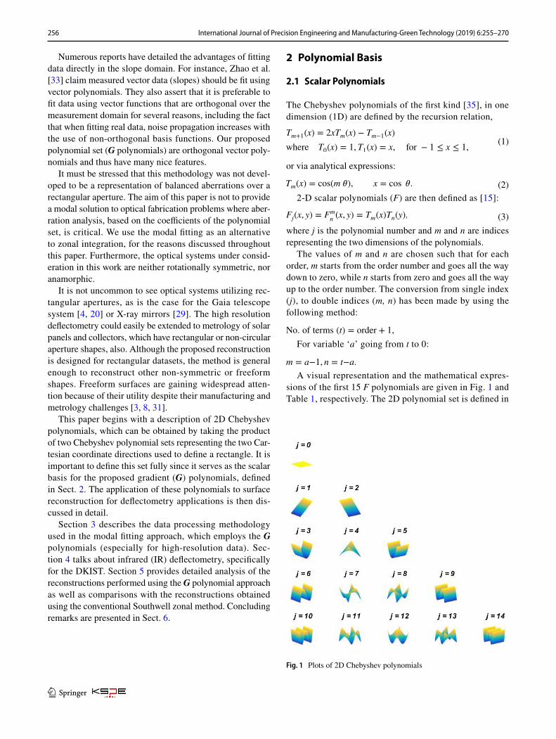
A visual representation and the mathematical expres-sions of the first 15 F polynomials are given in Fig. 1 and Table 1, respectively. The 2D polynomial set is defined in

(1)Tm+1(x) = 2xTm(x) − Tm−1(x)

where T0(x) = 1, T1(x) = x, for − 1 ≤ x ≤ 1,

(2)Tm(x) = cos(m �), x = cos �.

(3)Fj(x, y) = Fmn(x, y) = Tm(x)Tn(y),

No. of terms (t) = order + 1,

m = a−1, n = t−a.

Fig. 1 Plots of 2D Chebyshev polynomials

257International Journal of Precision Engineering and Manufacturing-Green Technology (2019) 6:255–270

1 3

both the x and y directions on the interval from −1 to +1. These definitions are similar to those in Ref. [15].

Chebyshev polynomials have several interesting prop-erties that make them attractive for data fitting, especially for discrete data. In addition to their orthogonal properties as defined in Refs. [15, 35], there are many cases in which the discrete orthogonality of Chebyshev polynomials can be shown to hold exactly [18]. For example Chebyshev poly-nomials of the first kind, Tm(x), m = 0, 1, 2,… ,N are orthogonal over the discrete point set comprising the zeros xN+1,m = 1, 2,… ,N + 1, of Tm+1(x) [1].

Additionally, Chebyshev polynomials can be used as an approximation to the minimax polynomial, for which the maximum value of the error between the function and its pol-ynomial approximation, is a minimum within some specified range [5]. Also, of all expansions in terms of ultra-spherical polynomials, the Chebyshev series generally has the fastest rate of convergence [5].

2.2 Gradient Polynomials

Among the most valuable properties of Chebyshev polynomi-als are the facts that their derivatives are orthogonal and they can be generated recursively. In 1-D, the gradients are given by,

(4)

T �

m(x) =

m[

Tm−1(x) − xTm(x)]

(

1 − x2) ,

T �

n(y) =

n[

Tn−1(y) − yTn(y)]

(

1 − y2) .

It is also interesting to note that the derivatives of the Chebyshev polynomials of the first kind are closely related to Chebyshev polynomials of the second kind [22], via the relation:

As for Chebyshev polynomials of the first kind, discrete orthogonality relations can be defined for the weighted Chebyshev polynomials of the second kind (where the weighting function is

√

1 − x2 ) [18].By taking the derivatives of the F polynomial set, the

G polynomials are obtained as follows:

The G polynomials can be written in terms of the recur-sive T polynomials as follows,

or in terms of Chebyshev polynomials of the second kind:

Table 2 lists the first 15 G polynomials and quiver plots of the first few non-trivial G polynomials are provided in “Appendix 1”. Orthonormality of the G polynomials is provided in “Appendix 2”. Each gradient term is a com-bination of two terms, each containing one scalar Cheby-shev polynomial ( Tm or Tn ) and one Chebyshev polynomial derivative term ( T ′

m or T ′

n ). This table was simplified using

the following relations:

Both T and U polynomials have simple, recursive rela-tionships [35]. Since the G polynomials can be expressed as a closed form equation involving the T and U polynomi-als, it is very straightforward and computationally efficient to generate them. This is a significant advantage for data processing since it enables large numbers of terms of the polynomials to be evaluated efficiently and reliably even if computing resources are limited. For T polynomials, the difference between recursive and direct calculation is only

(5)Um−1(x) =1

mT �

m(x) =

sin(m �)

sin(�), x = cos �.

(6)

Gj(x, y) = Gmn(x, y) = ∇Fm

n(x, y)

=𝜕

𝜕xFmn(x, y)i +

𝜕

𝜕yFmn(x, y)j,

Gj(x, y) = Tn(y)T�

m(x)i + Tm(x)T

�

n(y)j.

(7)

Gj(x, y) =m

2y(

1 − x2)

(

Tn+1(y) − Tn−1(y))(

Tm−1(x) − xTm(x))

i

+n

2x(

1 − y2)

(

Tm+1(x) − Tm−1(x))(

Tn−1(y) − yTn(y))

j,

(8)Gj(x, y) = m Tn(y)Um−1(x)i + n Tm(x)Un−1(y)j.

(9)T0(x) =1, T0(y) = 1; T1(x) = x, T1(y) = y;

T �

0(x) =0, T �

0(y) = 0; T �

1(x) = 1, T �

1(y) = 1.

Table 1 2D Chebyshev polynomials

j m n Fj(x, y) Explicit form of Fj(x, y)

0 0 0 T0(x)T

0(y) 1

1 1 0 T1(x)T

0(y) x

2 0 1 T0(x)T

1(y) y

3 2 0 T2(x)T

0(y) 2x2 − 1

4 1 1 T1(x)T

1(y) xy

5 0 2 T0(x)T

2(y) 2y2 − 1

6 3 0 T3(x)T

0(y) 4x3 − 3x

7 2 1 T2(x)T

1(y)

(

2x2 − 1)

y

8 1 2 T1(x)T

2(y)

(

2y2 − 1)

x

9 0 3 T0(x)T

3(y) 4y3 − 3y

10 4 0 T4(x)T

0(y) 8x4 − 8x2 + 1

11 3 1 T3(x)T

1(y)

(

4x3 − 3x)

y

12 2 2 T2(x)T

2(y) (2x2 − 1)(2y2 − 1)

13 1 3 T1(x)T

3(y) (4y3 − 3y)x

14 0 4 T0(x)T

4(y) 8y4 − 8y2 + 1


1 3

10−11, for a polynomial order of 20,000, generated over a grid of 50,000 points.

3 High‑Resolution Gradient Data Processing Using G Polynomials

Modal integration using the G polynomials is discussed in detail by describing the reconstruction process step by step.

3.1 Modal Fit of Gradient Data

Assume the surface (or wavefront) can be represented as,

where aj are the expansion coefficients, which need to be determined for a given data set.

Similarly, to represent the measured gradient, the following relation can be employed:

(10)W(x, y) =

N∑

j=1

ajFj,

where bk are the vector expansion coefficients of the G polynomials.

For discrete data, we can represent the modal fitting as a matrix [17]

where D is a column vector of P data values, b is a column vector containing the N expansion coefficients, and G is a P × N matrix representing the values of the G polynomials at the locations of the data points.

The coefficients can then be found using a pseudo-inverse:

These b coefficients and the associated G polynomi-als represent a best-fit estimate of the surface we wish to reconstruct.

(11)∇W(x, y) =

N∑

k=1

bkGk,

(12)D = Gb,

(13)b =

(

GTG)−1

GTD.

Table 2 Chebyshev gradient polynomials

j m n Explicit form of Gj(x, y) Gj(x, y) in terms of Fj(x, y)

0 0 0 0i + 0j 0

1 1 0 i T0(y)[T0(x)−xT1(x)]

(1−x2)i

2 0 1 j T0(x)[T0(y)−yT1(y)]

(1−y2)j

3 2 0 T �2(x)i 2

T0(y)[T1(x)−xT2(x)]

(1−x2)i

4 1 1 yi + xj T1(y)[T0(x)−xT1(x)]

(1−x2)i +

T1(x)[T0(y)−yT1(y)]

(1−y2)j

5 0 2 T �2(y)j 2

T0(x)[T1(y)−yT2(y)]

(1−y2)j

6 3 0 T �3(x)i 3

T0(y)[T2(x)−xT3(x)]

(1−x2)i

7 2 1 yT �2(x)i + T

2(x)j 2

T1(y)[T1(x)−xT2(x)]

(1−x2)i +

T2(x)[T0(y)−yT1(y)]

(1−y2)j

8 1 2 T2(y)i + xT �

2(y)j T

2(y)[T0(x)−xT1(x)]

(1−x2)i + 2

T1(x)[T1(y)−yT2(y)]

(1−y2)j

9 0 3 T �3(y)j 3

T0(x)[T2(y)−yT3(y)]

(1−x2)j

10 4 0 T �4(x)i 4

T0(y)[T3(x)−xT4(x)]

(1−x2)i

11 3 1 yT �3(x)i + T

3(x)j 3

T1(y)[T2(x)−xT3(x)]

(1−x2)i +

T3(x)[T0(y)−yT1(y)]

(1−y2)j

12 2 2 T2(y)T �

2(x)i + T

2(x)T �

2(y)j 2

T2(y)[T1(x)−xT2(x)]

(1−x2)i + 2

T2(x)[T1(y)−yT2(y)]

(1−y2)j

13 1 3 T3(y)i + xT �

3(y)j T

3(y)[T0(x)−xT1(x)]

(1−x2)i + 3

T1(x)[T2(y)−yT3(y)]

(1−y2)j

14 0 4 T �4(y)j 4

T0(x)[T3(y)−yT4(y)]

(1−y2)j


1 3

3.2 Obtaining Scalar Coefficients Directly from Gradient Data

Based on the method employed in the circular vector data papers by Zhao and Burge [33, 34], a simple conversion from G polynomial coefficients to F polynomial coefficients (see Eq. 3) is derived.

Denoting sets of vector and scalar data as V and S, respec-tively, the data sets can be expanded in terms of vector and scalar polynomial sets as follows:

where

Following the above definitions, the vector data can be expressed as,

Then, the coefficients of the scalar and vector polynomi-als can be related as,

Thus, there is a one-to-one correspondence between the coefficient sets, which makes the G polynomials unique and powerful in terms of reconstructing surface/wavefront maps. Once the slope data is fit to G polynomials, the surface uses the same coefficients applied to the F polynomials defined in Eq. 3.

4 Deflectometry for DKIST

A deflectometry system is a metrology tool which directly measures surface slope of a test optic. Surface reconstruction therefore requires an integration routine such as the method discussed above. As we show in Sect. 5, G polynomials are a particularly useful method for reconstructing surface shape from a deflectometry measurement.

Two in-house deflectometry systems have been developed and utilized for situations requiring high spatial resolution and large dynamic range freeform surface metrology [28, 30]. These systems are essentially computerized reverse Hartmann tests operating in the visible and long infrared wavelengths, and have been used to analyze high dynamic range tests of freeform surfaces [26]. A schematic of the infrared measurement scheme is shown in Fig. 2. A rectan-gular tungsten ribbon is heated to create a long wave infrared source, and is scanned in the x and y orthogonal directions. The camera focused on the mirror surface, records the reflec-tions from the test mirror surface for both scans, and by

(14)V =∑

bk��Gk ; S =

∑

akFk,

(15)��V = ∇S ; ��G = ∇F.

(16)��V =∑

bk��Gk = ∇S =

∑

ak(∇Fk) =∑

ak��Gk.

(17)ak = bk. knowing the system geometry, the local surface slopes in the x and y directions are calculated.

In these systems, the measured slopes are integrated to obtain the sag map of the surface under test. While histori-cally the slopes were integrated using a zonal method [24], a polynomial fitting method has also been attempted. The older polynomial approach proved impractical at providing high spatial resolution due to the inability to compute suf-ficient number of terms.

4.1 DKIST Primary Mirror Metrology

The Daniel K. Inouye Solar Telescope (DKIST) is designed to provide greatly improved optical performance in imaging, and spatial and spectral resolution when measuring dynamic solar phenomenon.

The SLOTS system was used to guide fabrication of the DKIST primary mirror during the grinding phase. Over this period a 25 µm down to 12 µm loose grit abrasive was used to grind the mirror, and the root-mean-square shape error was reduced from 15 µm to less than 1 µm [10]. The DKIST primary presented a unique freeform shape to measure, being a 4.2 m off-axis parabolic mirror constructed from Zerodur®. The full mirror specifications are provided in Table 3.

The SLOTS system used for testing consisted of a 4 mm wide tungsten wire which, when current was applied, would emit as a black body radiator. This wire served as the source for the deflectometry system. A micro-bolometer camera was utilized with an aperture diameter of 14 mm, and a peak

Fig. 2 Schematic diagram of the SLOTS deflectometry concept. LWIR stands for long-wave infrared [11]

Table 3 DKIST 4.2 m primary mirror optical parameters29

Optical parameters Value Note

Radius of curvature 16 mConic constant − 1.00 ParabolicOff-axis distance 4 m From parent vertexClear aperture diameter 4.2 mAspheric departure ~ 9 mm Peak-to-valley


1 3

absorption band of 7–11 µm. The camera and source were placed near the center of curvature of the DKIST primary mirror, at 17.1 m from the surface in a test tower. The wire was scanned in orthogonal x and y directions, and as long-wave IR light was emitted from the wire it would reflect from the mirror surface and be recorded by the camera sys-tem. Figure 3 shows the camera used with the SLOTS sys-tem. The schematic of the entire system was shown in Fig. 2.

In order to obtain slope data the local slopes in both x and y were calculated by ray tracing from the wire, to the mirror surface, to a camera detector pixel. This process was performed for all camera pixels, which were mapped to the mirror surface and served as discrete ‘pixel’ areas on the mirror over which the local slopes in x and y were calcu-lated. To achieve this, the Cartesian coordinates of the wire, camera, and mirror had to be known, as well as the camera mapping function. The Cartesian coordinates of all com-ponents were measured by using a laser tracker [6], which provided accuracy in position to within 0.1 µm. Additionally, the wire position during scans in both the x and y directions was recorded, again with the laser tracker. To determine the camera mapping function, reflective fiducials were placed on the mirror and the centroid position of the fiducials was calculated with the SLOTS system. This was a key step in the calibration process, and also was one of the most time consuming steps as the fiducials had to subsequently be removed, due to the integration method used at the time for surface reconstruction, which could not account for miss-ing data regions that the fiducials represented for the mirror surface. The calculated coordinates were compared with a laser tracker measurement of the true centroids to determine the camera distortion. With this information, along with the full system parameters, listed in Table 4, a theoretical cer-tainty of 8.5 µrad could be achieved for the calculated local slopes [25].

Fabrication of the DKIST primary mirror was per-formed by the College of Optical Sciences at the Univer-sity of Arizona. During the fine grinding stage deflectom-etry systems provided sub-micron accuracy for the entire non-specular, ground, freeform surface metrology [9, 11]. Multiple measurements were performed over the course of the mirror fabrication with this SLOTS system, and the raw data was all preserved. This served as an ideal source for real world slope data, which previously had been reconstructed into surface sag via a traditional South-well integration [24] method.

To evaluate the novel modal reconstruction method, this raw slope data was reconstructed using the new G polyno-mials based method, and is presented along with the origi-nal surface reconstruction results. The data fitting method-ology follows the procedure outlined in Sect. 3. Gradient data obtained from deflectometry is fit with the desired number of G polynomials, using Eqs. 12 and 13. Vector polynomial coefficients (referred to as ‘b’ in Sect. 3) thus obtained are converted to coefficients of the scalar poly-nomials (called ‘a’ in Sect. 3). In the case of our basis sets, the scalar and vector coefficients have a one-to-one correspondence (as seen from Sect. 3.2). Lastly, the ‘a’ coefficients and scalar basis set (F) are used to obtain the measured surface, using Eq. 10.

5 Performance Analysis

To evaluate the proposed modal method, we analyze its performance using several simulated and actual data sets. We discuss the results in terms of several figures of merit, such as the fit accuracy, performance in the presence of noise, processing time and the effectiveness of reconstruc-tion obtained with local obscuration cases.

It should be noted that all simulated data had gradi-ents generated by MATLAB’s ‘gradient’ function. This function uses correlations between pixels to determine the local slope, and therefore exact reconstruction is not

Fig. 3 The infrared microbolometer camera used with the SLOTS set-up

Table 4 Parameters in the DKIST SLOTS test

The surface is ground with 12 um grits (700 nm RMS roughness)

Parameter Value Unit

Power total consumed 44 WSource surface area 6280 mm2

Source width 4 mmCamera aperture diameter 14 mmCamera focal length 35 mmDetector pixel area 6.25 × 10−4 mm2


1 3

possible unless the slope integration assumes the same correlations. Neither the Southwell nor G polynomial method assumes these specific correlations and therefore we do not expect perfect reconstruction even though the data is simulated.

5.1 Fit Accuracy

We describe the modal method’s reconstruction accuracy and compare its results to ideal or Southwell reconstructed data.

5.1.1 Fitting Accuracy Evaluation Using Synthetic (Ideal) Data

We start by demonstrating how a simulated data set can be reconstructed accurately using G polynomials. A data set described by the following equation was generated in MAT-LAB in a 250 × 250 point grid:

The gradient of the data set was then reconstructed in two ways: modally using G polynomials (with the first 100 polynomials) and zonally using Southwell integration. The reconstruction results are compared with the ideal (MAT-LAB-simulated) surface in Fig. 4. Both results are nearly identical in this ideal case. The modal fitting residual error is 4.9799 × 10−4 µm (0.0108% error relative to the surface RMS of the ideal map) versus 5.1335 × 10−4 µm (0.0112% error relative to the RMS of the ideal map) for Southwell integration.

For this reconstruction, Southwell integration was a little faster, taking 0.389 s while G polynomial processing took 0.830 s.

5.1.2 Fitting Accuracy Evaluation Using Actual (Measured) Data

To test practical applicability, we applied G polynomials to actual deflectometry data (2.4 × 2.4 m sub-area) [11, 27] which includes noise, uncertainties, and other measurement

(18)

z(x, y) = 3.57x + 6.53x2 + 4.29y2 − 4.75y3 + 2.99(x3 + xy2)

− 2.95(2x4 + y4 + 2x2y2) + 1.21(x5 + xy4) + 0.89y5. errors. The analyzed data had an area of 201 × 201 pixels. The surface reconstruction was performed using the G poly-nomials as well as the standard Southwell integration pro-cess. The results of the two methods are compared in Fig. 5.

Even when only the first 37 terms of the G polynomi-als are used, an RMS difference between the two meth-ods of only 0.0183 µm is obtained. This corresponds to about 0.2327% of the RMS of the reconstructed surface or 0.0478% of the 38.3154 µm surface. It took 0.153 s for the G polynomial reconstruction versus 0.238 s with Southwell reconstruction, making the modal method a bit faster in this case.

Predictably, increasing the number of G polynomials terms, increases the reconstruction performance, as shown in Table 5, which lists the RMS values of the difference maps between the modal and Southwell surfaces. The Southwell surface was used as the reference surface.

Fig. 4 Surface plots of a simu-lated ideal surface, b G-polyno-mial-reconstructed surface, and c Southwell integrated surface

Fig. 5 Comparison of a G-polynomial-reconstructed and b Southwell integrated surfaces

Table 5 RMS Values of the differences between the Southwell (i.e., reference) and modal reconstructions; generated using different num-bers of modal terms

Number of G polynomials 15 50 150 500

RMS of difference map (µm) 0.0782 0.0095 0.0039 0.0021[RMS of difference map/RMS

of reference map] × 100 (%)0.9943 0.1208 0.0496 0.0267


1 3

5.1.3 Fidelity Check of Mid‑to‑high Spatial Frequency Reconstruction

To examine mid-to-high spatial frequencies, an arbitrary 1.2 × 1.2 m sub-section of the measured DKIST high-resolution data set was used. A high-pass Gaussian filter was applied to both the modally and zonally reconstructed surfaces, using SAGUARO data processing software [23], in order to focus on the high spatial resolution features in this case study. For the modal fit, a series of data sets were reconstructed, each of which was generated using a different number of G polynomials. These different high-pass-filtered G-polynomial surfaces are compared with the reference high-pass-filtered Southwell surface in Fig. 6.

From left to right in Fig. 6b–e (i.e., as the number of modal terms increases), the maps become less blurry and more high-frequency features become sharp and can be resolved. The graphs towards the right closely resemble the Southwell surface in Fig. 6a.

As expected, the representations of high frequencies improved as more terms were used for fitting. This finding emphasizes one of the critical advantages of the G polyno-mial set over others, namely, the ability to generate many thousands of terms. The simple recursion relations ensure that it is easy and practical to generate all of these high-order terms.

In principle, this data set could have been reconstructed with other basis sets, such as a Zernike-basis vector set, orthogonalized over a rectangular pupil [14]. However, that does not have a straightforward closed-form relationship which makes it difficult to generate such extreme orders. For high-resolution and freeform optics metrology and data processing applications, it is essential to use a suffi-cient numbers of polynomials. Additionally, there are sev-eral potential problems in converting Zernike polynomials to their gradients, orthogonalizing the Zernike gradients over a rectangular aperture, and generating the conversion matrices for obtaining the scalar coefficients from the vector fitting. This process is cumbersome, and has the possibil-ity to generate numerical errors, due to the several steps of computation, approximations and numerical truncations. As mentioned earlier, the metrology systems under considera-tion here are neither rotationally symmetric nor anamorphic,

so the balanced aberration representations of Zernike-type [14] or Legendre polynomials [16] are not necessarily valid.

5.2 Robustness Against Noise

This subsection describes the reconstruction performance in the presence of noise. Varying amounts of Gaussian white noise were added to the simulated ideal data set defined by Eq. (18). This “noisy” data was reconstructed using both the Southwell and modal (using the first 100 polynomials) approaches. In Fig. 7, the error in each reconstructed data set (difference between the ideal and reconstructed maps) as a percentage of the RMS of the ideal (noiseless) surface is plotted against the standard deviation of the added noise.

The polynomial fit error is smaller than the Southwell integration error for all noise levels. Furthermore, the per-formance of the Southwell method decreases faster as the amount of noise increases. For example, when the standard deviation of the noise is 0.2 µm, the polynomial fit exhibits an error of about 0.1% (relative to the RMS of the ideal surface), while the Southwell fit exhibits an error of about 0.5% (relative to the RMS of the ideal surface). These errors increase to 0.4% for the polynomial fit and 2.5% for the Southwell fit when the standard deviation of the noise is 0.5 µm.

Fig. 6 a Reference high-pass-filtered Southwell map and high-pass-filtered modal recon-structed maps generated using b 37, c 750, d 3000, and e 20,000 polynomial terms

Fig. 7 Residual errors from surface reconstruction in the presence of various amounts of noise


1 3

5.3 Reconstruction with Local Obscurations

When gradient data is processed using Southwell zonal inte-gration, issues such as mirror/lens surface defects, distortion correction fiducials, non-uniform data point distribution due to imaging distortion, and the presence of multiple local clear apertures can cause local obscurations in the data. Any areas with missing data that are encountered during the inte-gration process affect their surrounding regions. Although some numerical methods can be employed to reduce this effect (like replacing the missing data with zeros), the nature of the zonal approach fundamentally limits the reconstruc-tion accuracy when a sub-region is not well-defined. In con-trast, modal reconstructions are not significantly impacted by obscurations since they are based on overall views of the data.

For this analysis, a 250 × 250 pixel grid of synthetic data was simulated, and Fig. 8 shows the reconstruction results obtained when a small defect (a 90 × 2 pixel line of NaN (non-number) values, corresponding to an area of 90 × 2 mm) was added to this simulated data. After

reconstructing the data set using both the Southwell and modal approaches (with 2000 polynomial terms), the differ-ences between the results and the ideal scalar data are com-pared. Large differences are observed near the missing data.

The simulated ideal surface has an RMS of 95.1220 µm. The Southwell residual error map (difference between Southwell reconstructed and simulated surfaces) has an RMS of 0.8387 µm (or 0.8817% relative to the RMS of the simulated surface), whereas the modal error map has an RMS of 0.0627 µm (0.0659% error relative to the simu-lated surface. Thus, the residual error of the Southwell method is about 13 times higher than that of the modal method in this case.

Table 6 lists the RMS errors of the difference maps for the modal fits (i.e., the differences of the modal fits from the ideal surface) that were obtained using different number of polynomial terms. As expected, the RMS error decreases as the number of terms used in the expansion increases.

If an optic has multiple obscurations, Southwell zonal integration becomes more limited. Fiducials are one exam-ple, and are typically created by placing physical markers on the surface of the optic, essentially blocking parts of it. Ref. [19] provides an example of using fiducials for system calibration as a step in deflectometry. An actual picture of the DKIST mirror with fiducials placed on it during metrology is shown in Fig. 8d [2]. In this analysis, we added a few rectangular masks modelling fiducial areas to the same data that were used to generate Fig. 7. Each mask had dimensions of 24 × 30 pixels, corresponding to

Fig. 8 a Simulated ideal data with a 90 × 2 mm obscuration. b Southwell and c modal residual error maps (differences from the simulated map)

Table 6 RMS residual errors of the differences between the simulated and modal reconstructions

Number of G polynomials 100 500 1000 2000 3000

RMS error (µm) 1.4374 0.5032 0.0739 0.0627 0.0568[RMS of difference

map/RMS of ideal map] × 100 (%)

1.5111 0.5290 0.0777 0.0659 0.0597

Fig. 9 a Simulated ideal data with 24 × 30 mm fiducial masks. b Southwell and c modal residual error maps (differences from the simulated map). d Picture of fiducials on the DKIST mirror during a metrology run


1 3

24 × 30 mm. The simulated data and residual errors of the Southwell and modal (with 2000 polynomial terms) recon-structions with these fiducials are presented in Fig. 9a–c.

The RMS of the ideal surface in Fig. 8 is 93.8532 µm. The residual RMS error for the Southwell map is 5.9627 µm (or 6.3532% relative to the RMS of the ideal surface), whereas that for the modal fit is 0.7684 µm (or 0.8187% error). In this case, the Southwell error is about eight times higher than the modal error.

5.4 Comparison of Reconstruction Accuracy and Processing Time

This section aims to compare reconstruction accuracy and processing time between three methods (a) Zernike gradi-ent polynomial based modal method, from Refs. [33] and [34], (b) Southwell zonal method, and (c) G polynomial based modal method.

The simulated data is a freeform shaped wavefront, generated over a 200 × 200 point grid, representing a rec-tangular pupil with a mask pattern. The wavefront is of the form:

Using 30 polynomials each for both modal methods, the RMS error between the ideal wavefront and its recon-structions is given in Table 7. The G polynomial based

(19)W(x, y) = 0.14x2 − 0.33y5+1.89(3x2y − y3)

+ 0.57(x6 − 10x4y2 + 13x2y4 − y6).

reconstruction performs better than the other two meth-ods. Figure 10 shows the wavefront and its reconstruc-tions from the three aforementioned methods.

It is also worthwhile to consider the time it takes for the three methods to process data. Figure 11 shows the reconstruction time as the number of polynomials used

Table 7 RMS Error between the simulated wavefront (0.6792 µm RMS) and its various reconstructions

Wavefront Zernike gradient (modal)

Southwell (zonal) G polynomial (modal)

RMS of difference map (µm) 0.0745 0.0775 0.0379[RMS of difference map/RMS of ideal

map] × 100 (%)10.9625 11.4082 2.5698

Fig. 10 a Simulated ideal data. b Zernike gradient, c Southwell and d G Polynomial based modal residual error maps (differences from the simulated map)

Fig. 11 Plot of change in reconstruction time as the number of pol-ynomials used for data fitting is increased, for both modal methods. We acknowledge that the actual processing time could depend on the specific numerical implementation. This data is provided only for a baseline comparison


1 3

for the modal methods is increased. Data is shown only up to the 180th polynomial term because for higher polyno-mial terms, the Zernike gradient polynomial based modal fit becomes numerically unstable.

6 Conclusion

A complete and computationally efficient vector polyno-mial set, the G polynomial set, was derived. Chebyshev polynomials, which form the basis for the G polynomi-als, have several properties which make them an attractive choice to base our modal fitting method on.

One major advantage of the G polynomial approach is that both the scalar and vector polynomials are easy to define and manipulate and have a very simple relationship that ensures that the coefficients of the polynomials in both sets are the same. Hence, conversion between the two sets is straightforward. In addition, the G polynomials can be eas-ily computed, so even very high polynomial orders can be generated with high numerical efficiency. Since hundreds of thousands of polynomials can be generated, mid-to-high spa-tial frequencies of surfaces can be reconstructed from high-resolution-metrology data, such as was demonstrated for the

Daniel K. Inouye Solar Telescope (DKIST) mirror. Other advantages of this modal approach include better accuracy of reconstruction in the presence of scratches and fiducials.

Acknowledgements This material is partly based on work performed for the DKIST. DKIST is managed by the National Solar Observatory, which is operated by the Association of Universities for Research in Astronomy Inc. under a cooperative agreement with the National Sci-ence Foundation. Also, it is based in part upon work performed for the “Post-processing of Freeform Optics” project supported by the Korea Basic Science Institute. The deflectometry related software develop-ment is partially funded by the II–VI Foundation Block grant.

Compliance with ethical standards

Conflict of interest On behalf of all authors, the corresponding author states that there is no conflict of interest.

Appendix

Appendix 1

See Fig. 12.


1 3

Appendix 2

Orthonormality of the vector gradient polynomials

G polynomial orthogonality can be observed by noting that the dot product of two G polynomials is orthogonal:

(A.1)

1

�−1

�

Gj(x, y) ⋅ Gj� (x, y)

�√

1 − x2√

1 − y2dxdy =

�

0, j ≠ j�

NG, j = j�.

Next, we demonstrate the G polynomials’ orthonormality using the expanded form of the polynomials (from Eq. (7)):

where m, m′, n, and n′ are integers used for indexing and NG is the normalization factor, which is given by,

(A.2)

1

NG

1

∬−1

⎡

⎢

⎢

⎢

⎣

�

Tn(y)T�

m(x)i + Tm(x)T

�

n(y)j

�

⋅

�

Tn�(y)T�

m�(x)i + Tm�(x)T

�

n�(y)j

�

√

1 − x2√

(1 − y2

⎤

⎥

⎥

⎥

⎦

dxdy = 𝛿mm�𝛿nn�,

Fig. 12 Quiver plots of a few gradient polynomials


1 3

The proof of this derivation and details on how to obtain the normalization factor are as follows:

The first integral I1 can be expressed as:

Then, the following substitutions and subsequent equa-tions can be used:

(A.3)NG =

⎧

⎪

⎪

⎪

⎨

⎪

⎪

⎪

⎩

�2n2

4, m = 0

�2m2

4, n = 0

�2

8

�

m2 + n2�

, otherwise

.

(A.4)

I =

1

∬−1

(Gj ⋅ Gj� )√

1 − x2√

1 − y2dxdy

=

1

∬−1

Tn(y)Tn� (y)T�

m(x)T �

m� (x)√

1 − x2√

1 − y2dxdy

+

1

∬−1

Tm(x)Tm� (x)T�

n(y)T �

n�(y)

√

1 − x2√

1 − y2dxdy.

(A.5)

I1 =

1

∬−1

Tn(y)Tn� (y)T�

m(x)T �

m� (x)√

1 − x2√

1 − y2dxdy

=

1

∫−1

Tn(y)Tn� (y)√

1 − y2

1

∫−1

T �

m(x)T �

m� (x)√

1 − x2dydx

Tm(x) = cos�

m cos−1(x)�

.

x = cos (t), dx = − sin (t)dt, sin (t) =√

1 − x2,

I1 =

1

∫−1

Tn(y)Tn� (y)√

1 − y2

0

∫�

m sin�

m cos−1(x)�

m� sin�

m� cos−1(x)�

sin (t)(− sin (t))dtdy,

(A.6)

I1 =

1

∫−1

(Tn(y)Tn� (y)√

1 − y2dy

�

−mm��

m cos (�m) sin�

�m��

m2 − m�2.

This integral goes to zero for all values of m and m’ (except for when m = m� ), since sin(�m) = 0 for all integer values of m. However, when m = m�,

Using the identity,

As before, sin(2�m) = 0 for all integer values of m. Thus,

Using the same substitutions as before,

Again using the trigonometric identity for the square of the sine function,

(A.7)I1 =

1

∫−1

Tn(y)Tn� (y)√

1 − y2

0

∫�

sin (mt) sin (mt)dtdy.

sin2 (x) =

1 − cos (2x)

2,

(A.8)

I1 =

1

∫−1

Tn(y)Tn� (y)√

1 − y2dy

�

−m2

2

�

sin (2�m)

2m− �

��

�mm� .

(A.9)

I1 =�mm�

2�mm�

1

∫−1

Tn(y)Tn� (y)√

1 − y2dy =�m2

2�mm�

1

∫−1

cos�

n cos−1(y)�

cos�

n� cos−1(y)�√

1 − y2dy.

y = cos (t), dy = − sin (t)dt, sin (t) =√

1 − y2,

(A.10)I1 =�m2

2�mm�

0

∫�

cos (nt) cos(

n�t)(

− sin2 (t)

)

dt.

(A.11)

I1 = −�m2

2�mm�

0

∫�

cos (nt) cos�

n�t�

�

1 − cos (2t)

2

�

dt

= −�m2

2�mm�

⎛

⎜

⎜

⎜

⎜

⎜

⎜

⎜

⎜

⎜

⎝

−1

4

⎧

⎪

⎪

⎨

⎪

⎪

⎩

sin�

��

n − n� − 2��

n − n� − 2+

sin�

��

n − n� + 2��

n − n� + 2

+sin

�

��

n + n� − 2��

n + n� − 2+

sin�

��

n + n� + 2��

n + n� + 2

⎫

⎪

⎪

⎬

⎪

⎪

⎭

−

�

n� cos (�n) sin�

�n��

− n sin (�n) cos�

�n��

n2 − n�2

�

⎞

⎟

⎟

⎟

⎟

⎟

⎟

⎟

⎟

⎟

⎠

.


1 3

This integral equals zero for all values of n and n’, except when n = n� , in which case the integral is,

All of the sine terms become zero since n is an integer, so,

Similarly for I2,

Now the original integral becomes:

Next we address the cases in which either m = 0 or n = 0. When m = 0, I1 = 0 since,

so

where we used the fact that

Following the same steps as before,

Similarly, for n = 0,

where m and n are in the original basis in the last two equations.

It can easily be seen that I = 0 when m = 0 and n = 0.

References

1. 18.3 Definitions. DLMF: 18.3 definitions. N.p., n.d. Web. Retrieved July 25, 2017 from http://dlmf.nist.gov/18.3.

(A.12)

I1 = −�m2

2�mm�

0

∫�

cos2 (nt)

(

1 − cos (2t)

2

)

dt

=�m2

4�mm�

[

{

2�n + sin (2�n)

4n

}

+

{

n sin (2�n)

4(

n2 − 1)

}]

�nn� .

(A.13)I1 =�2m2

8�mm��nn� .

(A.14)I2 =�2n2

8�mm��nn� .

(A.15)

I =�2m2

8�mm��nn�+

�2n2

8�mm��nn� =

�2

8�mm��nn�

(

m2 + n2)

.

T �

m� (x) = T �

m(x) = 0,

(A.16)I = I2 =

1

∬−1

T �

n(y)T �

n�(y)

√

1 − x2√

1 − y2dxdy,

(A.17)Tm� (x) = Tm(x) = 1.

(A.18)I =�2n2

4�mm��nn� .

(A.19)I =�2m2

4�mm��nn� ,

2. Daniel K. Inouye solar telescope. N.p., n.d. Web. Retrieved July 31, 2017 from http://dkist .nso.edu/.

3. Chung, S., Song, S. E., & Cho, Y. T. (2017). Effective software solutions for 4D printing: A review and proposal. International Journal of Precision Engineering and Manufacturing., 4, 359.

4. Els, S., Lock, T., Comoretto, G., Gracia, G., O’Mullane, W., Cheek, N., et al. (2014). The commissioning of Gaia. Proceed-ings of SPIE, 9150, 91500A.

5. Fox, L., & Parker, J. B. (1968). Approximation. Minimax and least-squares theories. Chebyshev polynomials in numerical anal-ysis (pp. 1–17). London: Oxford U Pr.

6. Franceschini, F., Galetto, M., Maisano, D., & Mastrogiacomo, L. (2014). Large-scale dimensional metrology (LSDM): From tapes and theodolites to multi-sensor systems. International Journal of Precision Engineering and Manufacturing, 15, 1739.

7. Jüptner, W., & Bothe, T. (2009). Sub-nanometer resolution for the inspection of reflective surfaces using white light. Proceedings of SPIE, 7405, 740502.

8. Kim, B. C. (2015). Development of aspheric surface profilometry using curvature method. International Journal of Precision Engi-neering and Manufacturing, 16, 1963.

9. Kim, D. W., Aftab, M., Choi, H., Graves, L., & Trumper, I. (2016). Optical metrology systems spanning the full spatial frequency spectrum, FW5G.4. Washington: Optical Society of America.

10. Kim, D. W., Su, P., Oh, C. J., and Burge, J. H., Extremely large freeform optics manufacturing and testing, In 2015 Conference on lasers and electro-optics pacific rim, (Optical Society of America, 2015), paper 26F1_1.

11. Kim, D., Su, T., Su, P., Oh, C., Graves, L., & Burge, J. (2015). Accurate and rapid IR metrology for the manufacture of freeform optics. SPIE Newsroom. https ://doi.org/10.1117/2.12015 06.00601 5.

12. Knauer, M. C., Kaminski, J., & Hausler, G. (2004). Phase measur-ing deflectometry: A new approach to measure specular free-form surfaces. Proceedings of SPIE, 5457, 366.

13. Li, M., Li, D., Jin, C., Yuan, X., Xiong, Z., & Wang, Q. (2017). Improved zonal integration method for high accurate surface reconstruction in quantitative deflectometry. Applied Optics, 56, F144–F151.

14. Li, M., Li, D., Zhang, C., Wang, Q., & Chen, H. (2015). Modal wavefront reconstruction from slope measurements for rectan-gular apertures. Journal of the Optical Society of America A, 32, 1916–1921.

15. Liu, F., Robinson, B. M., Reardon, P. J., & Geary, J. M. (2001). Analyzing optics test data on rectangular apertures using 2-D Che-byshev polynomials. Optical Engineering, 50(4), 043609–043618.

16. Mahajan, V. N. (2010). Orthonormal aberration polynomials for anamorphic optical imaging systems with rectangular pupils. Applied Optics, 49, 6924–6929.

17. Mahajan, V. N. (2013). Optical imaging and aberrations, Part III: Wavefront analysis . Bellingham: SPIE Press.

18. Mason, J. C., & Christopher, D. (2003). Handscomb. Chebyshev polynomials. Boca Raton: Chapman & Hall.

19. Oh, C., Lowman, A. E., Smith, G. A., Su, P., Huang, R., Su, T., et al. (2016). Fabrication and testing of 4.2 m off-axis aspheric primary mirror of Daniel K. Inouye solar telescope. Proceedings of SPIE Advances in Optical and Mechanical Technologies for Telescopes and Instrumentation II, 9912, 99120O.

20. Polidan, R. S., Breckinridge, J. B., Lillie, C. F., MacEwen, H. A., Flannery, M. R., Dailey, D. R., et al. (2015). An evolvable space telescope for future astronomical missions 2015 update. Proceed-ings of SPIE, 9602, 960207.

21. Primot, J., Rousset, G., & Fontanella, J. C. (1990). Deconvolu-tion from wave-front sensing: A new technique for compensating turbulence-degraded images. Journal of the Optical Society of America A. Optics and Image Science, 7, 1598–1608.

http://dlmf.nist.gov/18.3

http://dkist.nso.edu/

https://doi.org/10.1117/2.1201506.006015

https://doi.org/10.1117/2.1201506.006015


1 3

22. Rivlin, T. J. (1974). The Chebyshev polynomials. New York: Wiley.

23. Smith, G. A., Lewis, B. J., Palmer, M., Kim, D. K., Loeff, A. R., & Burge, J. H. (2012). Open source data analysis and visualiza-tion software for optical engineering. Proceedings of SPIE, 8487, 84870F.

24. Southwell, W. H. (1980). Wave-front estimation from wave-front slope measurements. Journal of the Optical Society of America A, 70, 998–1006.

25. Su, T. (2014). Asphercial metrology for non-specular surfaces with the scanning long-wave optical test system . Tucson: Uni-versity of Arizona (Academic).

26. Su, P., Khreishi, M. H., Su, T., Huang, R., Dominguez, M. Z., Maldonado, A., et al. (2013). Aspheric and freeform surfaces metrology with software configurable optical test system: A computerized reverse Hartmann test. Optical Engineering, 53(3), 031305–031316.

27. Su, T., Park, W. H., Parks, R. E., Su, P., & Burge, J. H. (2011). Scanning long-wave optical test system: A new ground optical surface slope test system. Proceedings of SPIE, 8126, 81260E.

28. Su, P., Parks, R. E., Wang, L., Angel, R. P., & Burge, J. H. (2010). Software configurable optical test system: a computerized reverse Hartmann test. Applied Optics, 49, 4404–4412.

29. Su, P., Wang, Y., Burge, J., Kaznatcheev, K., & Idir, M. (2012). Non-null full field X-ray mirror metrology using SCOTS: A reflec-tion deflectometry approach. Optics Express, 20, 12393–12406.

30. Su, T., Wang, S., Parks, R. E., Su, P., & Burge, J. H. (2013). Meas-uring rough optical surfaces using scanning long-wave optical test system. 1. Principle and implementation. Applied Optics, 52, 7117–7126.

31. Tan, G., Zhang, L., Liu, S., & Zhang, W. (2015). A fast and dif-ferentiated localization method for complex surfaces inspection. International Journal of Precision Engineering and Manufactur-ing, 16, 2631.

32. Tang, Y., Su, X., Liu, Y., & Jing, H. (2008). 3D shape measure-ment of the aspheric mirror by advanced phase measuring deflec-tometry. Optics Express, 16, 15090–15096.

33. Zhao, C., & Burge, J. H. (2007). Orthonormal vector polynomials in a unit circle, part I: Basis set derived from gradients of Zernike polynomials. Optics Express, 15, 18014–18024.

34. Zhao, C., & Burge, J. H. (2008). Orthonormal vector polynomials in a unit circle, part II: Completing the basis set. Optics Express, 16, 6586–6591.

35. Zwillinger, D. (2003). Special functions. CRC standard math-ematical tables and formulae (31st ed., pp. 532–538). Boca Raton: CRC.

Publisher’s Note Springer Nature remains neutral with regard to jurisdictional claims in published maps and institutional affiliations.

Maham Aftab is a Senior Design Engineer at ASML, US. She is also a doctoral candidate in the College of Optical Sciences, University of Arizona. Her research focuses on hardware and software design and analy-sis; and mathematical study and development for optical metrol-ogy systems, particularly for high-resolution and freeform optics.

James H. Burge is Professor Emeritus of Optical Sciences at the University of Arizona.

Greg A. Smith conducts research in large optics manufacturing and testing at the College of Optical Sciences, University of Arizona. He received his optics Ph.D. in 2006 and specializes in the areas of polarization optics and software algorithms for opti-cal metrology.

Logan Graves is a PhD candidate in the College of Optical Sci-ences at the University of Ari-zona. His main research area covers precision optical metrol-ogy, focusing on deflectometry hardware and software develop-ment for improved freeform measurement capabilities. He also has a background in bio-medical engineering, with research topics including early cancer detection utilizing auto-fluorescence and non-linear rod-cone interactions at the retinal level.

Dr. Chang‑jin Oh is the PI of Opti-cal Engineering and Fabrication Facility in College of Optical Sciences and he has provided leadership role to the group for the last 15 years. His expertise includes large scale optomechan-ical systems for space and ground base application, optical fabrication and precision metrol-ogy. He has been PI and Co-PI of various many challenging large optics projects for astronomy and


1 3

optics community as well as national and international science organi-zations. He has successfully managed many large optics projects including HET wide field corrector, Daniel K. Inoue Solar Telescope Primary mirror fabrication, 6.5m Primary fabrication and large aper-ture vacuum compatible reference optical systems.

Dae Wook Kim is an assistant professor of optical sciences and astronomy at the University of Arizona. He has been working in the optical engineering field for more than 10 years, mainly focusing on very large astronom-ical optics, such as the 25 m diameter Giant Magellan Tele-scope primary mirrors. His main research area covers precision freeform optics fabrication and various metrology topics, such as interferometric test systems using computer generated holo-grams, direct curvature measure-

ments, and dynamic deflectometry systems. He is currently a chair of the Optical Manufacturing and Testing conference (SPIE), Optical

Fabrication and Testing conference (OSA), and Astronomical Optics: Design, Manufacture, and Test of Space and Ground Systems confer-ence (SPIE). He is a senior member of OSA and SPIE and has been serving as an associate editor for the journal Optics Express.

modal data processing for high resolution deflectometry

Documents