mode-based frequency response function and steady state...

11th International LS-DYNA® Users Conference Simulation (3)

9-39

Mode-based Frequency Response Function and Steady State Dynamics in LS-DYNA®

Yun Huang1, Bor-Tsuen Wang2

1Livermore Software Technology Corporation 7374 Las Positas Rd., Livermore, CA, United States 94551

[email protected]

2Department of Mechanical Engineering College of Engineering

National Pingtung University of Science and Technology Pingtung, Taiwan 91207

[email protected]

Abstract

Two new features used for frequency domain structural analysis --- frequency response function (FRF) and steady state dynamics (SSD), have been implemented in LS-DYNA, based on mode superposition techniques.

As a characteristic of a structure, FRF is the transfer function which represents structural response resulting from applied unit harmonic excitations. The harmonic excitations can be given in the form of nodal force, base acceleration or pressure. The FRF feature provides user the opportunity to acquire a spectrum of structural response (displacement, velocity and acceleration) for the applied unit excitation. As a direct extension of FRF, SSD calculates the steady state dynamic response of a system subjected to a given spectrum of harmonic excitations. Both FRF and SSD give results in complex variable form, enabling user to obtain not only amplitude of response, but also phase angle.

A benchmark example of a rectangular plate is included to demonstrate the effectiveness of both features. Some discussions regarding the effect of damping and individual mode contributions are also included.

Introduction This paper introduces two new features of LS-DYNA: Frequency Response Function (FRF) and Steady State Dynamics (SSD). They are important tools in frequency domain analysis and have been widely used in various industries.

Frequency response function (FRF) is the characteristic of a structure that has a measured or computed response resulting from a unit harmonic input. Usually this function is given for a range of frequencies. The response can be given in terms of displacement, velocity, or acceleration. FRFs are complex functions, with real and imaginary components. They can also be expressed in the form of amplitude and phase angle pairs.

Steady state dynamics (SSD) feature calculates the steady state response of a structure subjected to harmonic excitations. The excitation spectrum can be given as nodal force, pressure or base accelerations. The excitation spectrum takes complex variable input. In other words, both the amplitude and the phase angle of the excitation can be considered.

Simulation (3) 11th International LS-DYNA® Users Conference

9-40

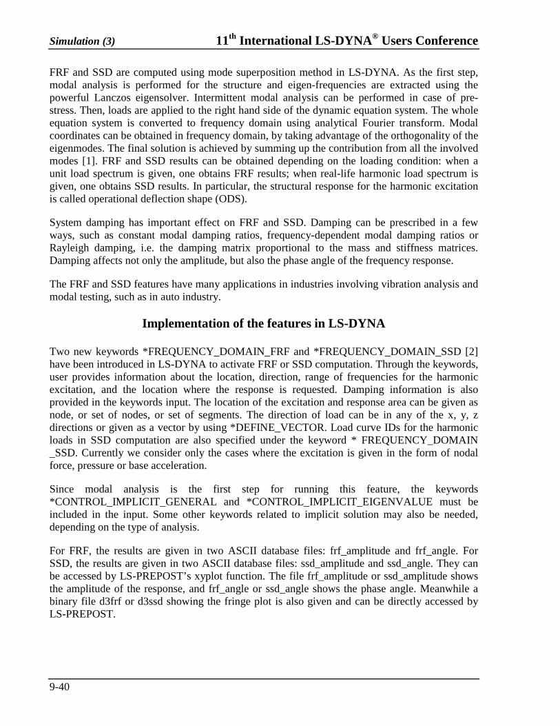
FRF and SSD are computed using mode superposition method in LS-DYNA. As the first step, modal analysis is performed for the structure and eigen-frequencies are extracted using the powerful Lanczos eigensolver. Intermittent modal analysis can be performed in case of pre-stress. Then, loads are applied to the right hand side of the dynamic equation system. The whole equation system is converted to frequency domain using analytical Fourier transform. Modal coordinates can be obtained in frequency domain, by taking advantage of the orthogonality of the eigenmodes. The final solution is achieved by summing up the contribution from all the involved modes [1]. FRF and SSD results can be obtained depending on the loading condition: when a unit load spectrum is given, one obtains FRF results; when real-life harmonic load spectrum is given, one obtains SSD results. In particular, the structural response for the harmonic excitation is called operational deflection shape (ODS).

System damping has important effect on FRF and SSD. Damping can be prescribed in a few ways, such as constant modal damping ratios, frequency-dependent modal damping ratios or Rayleigh damping, i.e. the damping matrix proportional to the mass and stiffness matrices. Damping affects not only the amplitude, but also the phase angle of the frequency response.

The FRF and SSD features have many applications in industries involving vibration analysis and modal testing, such as in auto industry.

Implementation of the features in LS-DYNA Two new keywords *FREQUENCY_DOMAIN_FRF and *FREQUENCY_DOMAIN_SSD [2] have been introduced in LS-DYNA to activate FRF or SSD computation. Through the keywords, user provides information about the location, direction, range of frequencies for the harmonic excitation, and the location where the response is requested. Damping information is also provided in the keywords input. The location of the excitation and response area can be given as node, or set of nodes, or set of segments. The direction of load can be in any of the x, y, z directions or given as a vector by using *DEFINE_VECTOR. Load curve IDs for the harmonic loads in SSD computation are also specified under the keyword * FREQUENCY_DOMAIN _SSD. Currently we consider only the cases where the excitation is given in the form of nodal force, pressure or base acceleration.

Since modal analysis is the first step for running this feature, the keywords *CONTROL_IMPLICIT_GENERAL and *CONTROL_IMPLICIT_EIGENVALUE must be included in the input. Some other keywords related to implicit solution may also be needed, depending on the type of analysis.

For FRF, the results are given in two ASCII database files: frf_amplitude and frf_angle. For SSD, the results are given in two ASCII database files: ssd_amplitude and ssd_angle. They can be accessed by LS-PREPOST’s xyplot function. The file frf_amplitude or ssd_amplitude shows the amplitude of the response, and frf_angle or ssd_angle shows the phase angle. Meanwhile a binary file d3frf or d3ssd showing the fringe plot is also given and can be directly accessed by LS-PREPOST.


9-41

Description of a benchmark example Consider a rectangular plate in Figure 1. The size of the plate is given as a = 0.36m, b = 0.24m, t = 0.002m. Material properties are given as density ρ = 7870 kg/m3, Young’s modulus E = 207×109 Pa, Poisson’s ratio γ = 0.292. Shell element type 6 (S/R Hughes Liu shell) is adopted. Totally 651 nodes and 600 shell elements are used for the modeling. Nodal force is applied at point A. For FRF, Accelerance (acceleration response for a unit force load) in the range of 1-400 Hz are computed and the modes with natural frequencies less than 2000 Hz are used in the computation. For SSD, displacement responses for a given spectrum of nodal force in the range of 10-140 Hz are computed.

A

B

a

b

t

Figure 1 – A rectangular plate with free boundaries

Validation of the results

Wang and Tsao performed experimental modal analysis (EMA) and finite element analysis (FEA) for this benchmark problem [3]. In the finite element analysis, the software ANSYS was adopted and the convergence for different elements was studied.

The natural frequencies of the plate obtained by LS-DYNA match reasonably well with the analytical, experimental and ANSYS results given by [3] (see Table 1). The only exception is the 4th mode, where the natural frequency given by experiments is around 6% away from the Analytical, ANSYS and LS-DYNA solutions. The possible reason may be that two small holes are introduced in the plate to hold it during the experiments, which may slightly change the vibration modes of the plate [3].

Mode Analytical Experimental ANSYS LS-DYNA

1 76.294 76.12 76.835 78.6163 2 81.865 83.00 81.624 81.3628 3 176.806 177.65 177.11 179.6108 4 190.602 201.50 189.88 188.6555 5 220.581 221.70 220.37 219.6902 6 255.791 261.41 254.96 255.1308 7 N/A 329.00 327.88 329.1959 8 N/A 383.23 377.43 379.2899

Table 1 – Natural frequencies of the plate (Unit: Hz)

FRF results at point A and point B are computed. When the response is computed at the point A (same as the excitation point) the function is called as the point FRF. When response is


9-42

computed at the corner point B (which is different from the excitation point) the function is called as the transfer FRF.

In Figures 2 and 3 the LS-DYNA results for Accelerance (acceleration/force) amplitude are compared with the results from [3] (experimental and ANSYS). A constant damping ratio ζ = 0.01 is adopted for both LS-DYNA and ANSYS computation. The peak responses always take place at the natural frequencies, as expected. For the amplitude, LS-DYNA results match reasonably well with ANSYS results for the whole range of frequencies. Both numerical results (LS-DYNA and ANSYS) match very well with the experimental results in the low frequencies (e.g. f < 280 Hz), but an increasing discrepancy is observed for high frequencies.

Figure 2 – Amplitude of accelerance at point A


9-43

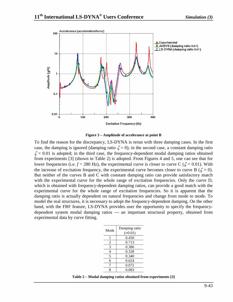
Figure 3 – Amplitude of accelerance at point B

To find the reason for the discrepancy, LS-DYNA is rerun with three damping cases. In the first case, the damping is ignored (damping ratio ζ = 0); in the second case, a constant damping ratio ζ = 0.01 is adopted; in the third case, the frequency-dependent modal damping ratios obtained from experiments [3] (shown in Table 2) is adopted. From Figures 4 and 5, one can see that for lower frequencies (i.e. f < 280 Hz), the experimental curve is closer to curve C (ζ = 0.01). With the increase of excitation frequency, the experimental curve becomes closer to curve B (ζ = 0). But neither of the curves B and C with constant damping ratio can provide satisfactory match with the experimental curve for the whole range of excitation frequencies. Only the curve D, which is obtained with frequency-dependent damping ratios, can provide a good match with the experimental curve for the whole range of excitation frequencies. So it is apparent that the damping ratio is actually dependent on natural frequencies and change from mode to mode. To model the real structures, it is necessary to adopt the frequency-dependent damping. On the other hand, with the FRF feature, LS-DYNA provides user the opportunity to specify the frequency-dependent system modal damping ratios ⎯ an important structural property, obtained from experimental data by curve fitting.

Mode Damping ratio

(×0.01) 1 0.450 2 0.713 3 0.386 4 0.328 5 0.340 6 0.624 7 0.072 8 0.083

Table 2 – Modal damping ratios obtained from experiments [3]


9-44

Figure 4 – Effect of damping on accelerance at point A

Figure 5 – Effect of damping on accelerance at point B

Contribution from each vibration mode or a particular group of vibration modes to the FRF or SSD results can be studied. Figures 6 and 7 show the accelerance at points A and B obtained by considering 1) all the modes with natural frequency f < 2000 Hz; 2) the first mode only; 3) the second mode only; and 4) the third mode only. Please note that the modes in 2), 3) and 4) refer to


9-45

non-rigid body modes. This modal contribution analysis may help diagnose the harmful vibration modes for machines or structures under operation or loads.

One can notice the resonance at each natural vibration mode in Figures 6 and 7. The contribution on structural response from each mode reaches the peak at its natural frequency and decay rapidly below and above the natural frequency. This fact enables us to use only a few of the vibration modes when computing FRF or SSD results for a given range of excitation frequencies. This may help reduce the CPU time, especially for large scale computations involving millions of elements and thousands of modes.

Figure 6 – Mode contribution at point A


9-46

Figure 7 – Mode contribution at point B

For SSD computation, a simple spectrum of nodal force is applied at point A. The nodal force spectrum is given in Appendix 1. The amplitudes of the displacement response given by LS-DYNA and by ANSYS are compared in Figures 8 and 9.

Figure 8 – Amplitude of SSD displacement response at point A


9-47

Figure 9 – Amplitude of SSD displacement response at point B

Generally speaking the response given by LS-DYNA and ANSYS matches well, except for the results at the excitation frequency 80 Hz. The reason for the discrepancy at frequency 80 Hz can be explained as follows. For the on-resonance or near-resonance excitation, the steady state response is dominated by the natural modes whose frequencies are closest to the excitation frequency. In this example, the two natural frequencies of the plate which are closest to 80 Hz are 78.616 Hz and 81.363 Hz from LS-DYNA, and 76.835 Hz and 81.624 Hz from ANSYS, respectively. Thus the plate response at frequency 80 Hz is expected to be dominated by the two modes (78.616 Hz and 81.363 Hz from LS-DYNA, and 76.835 Hz and 81.624 Hz from ANSYS). Comparing with the “dominating modes” from ANSYS, the two “dominating modes” from LS-DYNA are closer to the excitation frequency 80 Hz. Thus the plate is expected to have higher response values by LS-DYNA than by ANSYS, at the excitation frequency 80 Hz. The discrepancy on the natural frequencies obtained by ANSYS and LS-DYNA explains also why ANSYS provides higher response values than LS-DYNA does, at the excitation frequency 70 Hz.

Figures 10 and 11 show the contours of displacement response at the excitation frequency 80 Hz given by ANSYS and LS-DYNA, respectively. Though there is some discrepancy in the amplitude of the response, the distribution of the response by ANSYS and by LS-DYNA is still quite similar. In both results, the maximum response appears at node 334 and the minimum response appears at node 31.


9-48

Figure 10 – Displacement response contour at frequency=80 Hz (ANSYS)

Figure 11 – Displacement response contour at frequency=80 Hz (LS-DYNA)

Conclusion

Two new features of LS-DYNA, Frequency Response Function (FRF) and Steady State Dynamics (SSD) are introduced in the paper. The two features are useful in frequency domain analysis. They can find applications in the area of vibration analysis and modal testing.

A benchmark example of a rectangular plate is adopted to illustrate the effectiveness and accuracy of the implementation. The example also indicates that it is necessary to adopt frequency-dependent modal damping ratios for modeling real structures.


9-49

References

1. Bor-Tsuen Wang, Vibration Analysis of a Continuous System Subject to Generic Forms of Actuation Forces and Sensing Devices. Journal of Sound and Vibration, 319: 1222–1251 (2009).

2. LS-DYNA Keyword User's Manual, Version 971, Livermore Software Technology Corporation, 2010. 3. Bor-Tsuen Wang, Wen-Chang Tsao, Application of FEA and EMA to Structural Model Verification.

Proceeding of the 10th CSSV Conference Taiwan, 2002; 131-138.

Appendix

Appendix 1. Nodal force spectrum for SSD computation.

Frequency (Hz) Amplitude (N) Phase Angle (°) 10.0 10.0 0.0 20.0 12.0 0.0 30.0 14.0 0.0 40.0 16.0 0.0 50.0 18.0 0.0 60.0 16.0 0.0 70.0 12.0 0.0 80.0 13.0 0.0 90.0 15.5 0.0

100.0 16.5 0.0 110.0 15.5 0.0 120.0 18.5 0.0 130.0 15.5 0.0 140.0 10.5 0.0


9-50

mode-based frequency response function and steady state...

Documents