model 1133a phasor measurement specifications 1133a phasor measurement specifications arbiter...

Model 1133A Phasor Measurement Specifications

Arbiter Systems, Inc. · 1324 Vendels Circle, Suite 121 · Paso Robles, CA 93446 · USATel: +1.805.237.3831 · Fax: +1.805.238.5717 · E-mail: [email protected] · Internet: http://www.arbiter.com 1

Table 1: 1133A Phasor Measurement Specifications

1There is a limit on the total number of cycles calculated as follows: the value (R1*W1) + (R2*W2) must not exceed400. R1 and R2 are the phasor estimate reporting rates for virtual PMU #1 and #2, respectively and W1 and W2 are therespective window lengths in cycles. See example calculation under ‘Virtual PMU,’ next page. The maximum reportingrate of either 50 or 60 per second is only available on one PMU. If 50 or 60 per second is selected for a PMU the otherPMU must be configured for a lower rate.

2All corrections for internal offsets and system configuration (for example, PT and CT ratios and their errors) areperformed automatically and are included in the 0.1% limit. This limit presumes operation under specified conditions,including lock to a suitable time base such as GPS, and includes all errors resulting from such operation. See the Model1133A Technical Data for more information, including performance degradation caused by operation without a referencetime base.

3Voltages and currents may be selected independently for each virtual PMU. Voltages and currents are selected asa three-phase entity, i.e. selection of ‘voltage’ enables calculation for all three voltage inputs A, B and C. The per-phaseinputs are not individually selectable.

4Each of the three selectable blocks of data (per-phase, positive sequence, and negative/zero sequence) and fixed/floating point format may be independently selected for each virtual PMU. The separate phases and negative/zerosequence are not individually selectable. The selection of fixed- or floating-point applies to all selections for a given virtualPMU.

Number of virtual PMUs per unit. 2Each virtual PMU has its own ID number and configuration. Each PMUmay be disabled if not used.

Nominal centre frequency, F Adaptive tuning Bandwidth

50 or 60 HzSelectable, off or ±2, ±5, or ±10 Hz tracking limitSee discussion under Window Functions

Phasor estimate reporting rate, R1 At 50 Hz: 1, 2, 5, 10, 25, or 50/secondAt 60 Hz: 1, 2, 3, 4, 5, 6, 10, 12, 15, 20, 30, or 60/secondPhasor estimates are batch processed, 20 times per second

Window length, W1

Group delay

At 50 Hz: 1 to 16 nominal cycles (integer values)At 60 Hz: 1 to 16 nominal cyclesW/2F, in seconds

Estimator algorithm Selectable: Raised cosine per de la O and Martin, 2003 [1];Hann; Hamming, Blackman; Triangular (Bartlett); Rectangular; Flat Top;Kaiser; Nutall 4-term [3] (see section on Window Functions).

Measurement accuracy 0.1% Total Vector Error (TVE) maximum2, plus estimator error (generallysmall with proper configuration; can be modelled for suitability for aparticular application; see Selecting Windows and Their Parameters)

Input signals processed A, B, and C channel voltageA, B, and C channel current(both selectable on/off)1, 3

Phasor estimate reporting formats A, B, and C per-phase dataPositive-sequence componentNegative and zero-sequence components(each group selectable on/off)4

Fixed or floating-point4

Data formatting compatibility Per IEEE Standard C37.118-2005 [2], serial or Ethernet

Arbiter Systems, Inc. · 1324 Vendels Circle, Suite 121 · Paso Robles, CA 93446 · USATel: +1.805.237.3831 · Fax: +1.805.238.5717 · E-mail: [email protected] · Internet: http://www.arbiter.com


2

Model 1133A BackgroundThe Model 1133A Power Sentinel includes a flexible, floating-point digital signal processor (DSP). This powerful DSP

has allowed Arbiter Systems to significantly enhance functionality of the Model 1133A since its introduction. Theseenhancements are free to all users of the Model 1133A, requiring only a firmware download to enable the most recentfeatures. (Some early units require the installation of a new DSP boot ROM to enable firmware download. Contact thefactory for a free boot ROM if required.)

The initial implementation of phasor measurements in the Model 1133A was based on its 20/second commonmeasurement rate, used for all basic internal functions (voltage, current, power, frequency, etc.) This 20/second data,adequate for many applications, was simply output in phasor format. With the enhancements described here, variableupdate rates from 1 to 240/second are supported, with individually-selectable configuration parameters for each of twovirtual phasor measurement units (PMUs).

Latency: Although phasor estimates are now available at reporting rates of up to 60/second, the actual calculationand formatting of the results is still performed once every 50 ms, as each new input data block becomes available.

Therefore, latency estimates must include an allowance for thisbatch processing. Latency for each block can vary from (W/2F)+30 ms for the most recent phasor estimate to (W/2F)+80 msfor the oldest estimate within each batch. W and F are definedin the specification table above. W/2F is the inherent group delayof a symmetric FIR estimator. Keep in mind that latencyestimates are approximate, and can be significantly longerdepending on the communications channel. The numbers hereare for an Ethernet network without significant added delay dueto collisions. Latency is defined here as the time between thephasor time tag (at the middle of each window) and the time whendata transmission begins.

Virtual PMUThe virtual PMU is implemented as a separate processing

block in the DSP, based on a common set of sampled input datafrom the unit’s three-phase voltage and current input section(figure 1). The hardware is shared between the two virtual PMUs,but each has its own set of configuration parameters, all ofwhich, including the PMU ID field, can be selected completelyindependently of the other virtual PMU. It is even possible to setone PMU for 50 Hz operation and one for 60 Hz operation,although it is unlikely that such a combination would be veryuseful. However, in some applications, it is useful to havephasor data at different rates, or in different formats, or usingestimators optimised with different characteristics.

For instance, a Model 1133A could be configured with two virtual PMUs as follows. One PMU might measure dataat a once-per-cycle rate (50 or 60 phasors per second), giving floating-point results for all six inputs (three voltage + threecurrent), with a 4-cycle measurement window. This PMU could deliver its results via Ethernet for local controlapplications. A second PMU, optimised for wide-area monitoring (WAM), might provide phasor estimates at a lower rate,say 10/second, of positive-sequence voltage only, formatted in fixed point for transmission over a low-bandwidth channelto a remote phasor data concentrator. This PMU could use a longer window, 10 or 12 cycles long, with a correspondinglynarrower bandwidth to provide anti-aliasing. Adaptive centre-frequency tuning could be used in this PMU, to eliminaterolloff (magnitude errors) for off-nominal frequency signals, even with the narrower bandwidth.

For this example, the total number of calculated cycles is as follows (using 60 Hz for the example): R1 = 60/second;W1 = 4 cycles: R1*W1 = 240. R2 = 10/second; W2 = 12 cycles: R2*W2 = 120. 240 + 120 = 360, under the limit of 400.Similar results can be calculated for a 50 Hz system. So, the choice of parameters, particularly reporting rates, is not



usually limited by hardware capabilities, but can be optimised for the application. For example, you could change theconfiguration of virtual PMU #2, used for the WAM function, to provide data at a higher rate using a shorter window toprovide a wider measurement bandwidth when the wide-area network is updated, without affecting the configuration forvirtual PMU #1.

Window FunctionsThe Model 1133A offers a wide range of window functions. The choice can be optimised for each application. All

window functions serve the same purpose (as a low-pass filter) and work in the same basic way. The main differencebetween windows is the shape and magnitude of ‘sideband lobes,’ which are peaks in the rejection band. The variouswindow functions also have differences in passband width and flatness. Figures 2 and 3 show the in-band and rejectionresponses of several of the available windows. All of these windows are shown for F=60, W=4 except the rectangularwindow, which is shown for W=1 for comparison with first-generation PMUs, which used this function. For the raisedcosine window, K=2 and α=0.7. Curves for 50 Hz are similar, multiplying the frequency scale by 5/6.

Window functions are also called ‘weighting functions,’ because they work by multiplying the input signal time recordby an equal-length sequence of constants, or weighting factors. Most window functions decrease smoothly to zero attheir ends (see figure 4). The rectangular window is an exception: all of its values are 1.0, and it is equivalent to no windowat all. It has the narrowest main lobe (passband) of any window (for a given width), and works well only when the signalis centred in the passband, i.e. at nominal system frequency. Its performance is worse than any other window for off-nominal and out-of-band signals. The differences in rolloff between the various window functions become more apparentas the signal moves further from nominal (greater frequency offset).

Figures 2 and 3: Performance of selected window functions

Note that all windows in the Model 1133A offer variable width in terms of nominal power-system cycles, with windowlengths up to 320 ms available. The shortest practical window length varies and is generally longer for higher-performancewindows. This is a general characteristic of finite-impulse-response (FIR) filters, of which windowed estimators are oneexample: performance improves using longer windows, or equivalently, more data samples. ‘Performance’ here meansimproved in-band flatness, narrower transition band, and/or increased out-of-band rejection. However, as performancemeasured by these parameters improves, group delay increases.

For all window functions, as window length increases the passband narrows in inverse proportion (figure 5). Sidebandlobes also narrow and move closer to the passband, while their magnitude stays relatively constant. For some of thewindow functions (raised cosine and Kaiser), other constants also affect the shape and performance of the window. Forthe raised-cosine window, the 6-dB bandwidth is a function of the constants K and α, as well as the window length:passband width is proportional to K/W.



4

Figures 4 and 5: Window shape and effect of window length

All of the windows used in the Model 1133A are symmetric, which means that they have a constant group delay equalto half the window length, W/2F. Applications that need fast response must therefore accept tradeoffs in performancemeasured in the frequency domain. Where greater accuracy or more rejection is needed, and response time is lesscritical, the Model 1133A easily produces estimators based on longer, higher-performance windows that deliver theneeded accuracy.

Note that with adaptive tuning (see below), a broad passband is not required, since the estimator centre frequencyfollows the applied signal. The window function can be selected for its rejection and group delay characteristics only.Indeed, a narrower passband aids in rejecting noise.

References [3] and [4] provide good background on the derivation and use of window functions.

Selecting Windows and Their ParametersThe acceptance criteria for a window should include its 1% bandwidth (wider is better) and rejection at 2(F±∆F),

typically 100-140 Hz for a 60 Hz system, or 80-120 Hz at 50 Hz. To minimise errors due to feedthrough of this double-frequency term, rejection should be -40 dB minimum, and -60 dB is better. If anti-aliasing for low reporting rates is anissue, rejection will be important at much lower frequencies, as well.

For most applications, the rectangular and triangular (Bartlett) windows are not recommended, since the other windowsoffer superior performance. These two are provided mostly for experimental purposes. The often-used Hann (sometimescalled Hanning) and Blackman windows both have the desirable characteristic that the magnitude of their rejectionsidelobes decreases with increasing frequency. They also have reasonable passband characteristics, especially whenused with adaptive tuning, and where anti-aliasing is an issue. The Hamming window is similar to the Hann, but sincethe window does not go to zero at the ends, its rejection sidelobes do not decrease as quickly. The first sidelobe is,however, smaller than for the Hann. The Nutall 4-term window [3] is similar to the Hann and Blackman, with even betterrejection characteristics (>90 dB). The Hann and Hamming (2-term), Blackman (3-term) and Nutall (4-term) windows alluse the same general equation (as does the flat-top, discussed later). These are called the Blackman-Harris family ofwindows:

w(n) = a0 – a

1cos(2πn/N) + a

2cos(4πn/N) – a

3cos(6πn/N); 0 ≤ n ≤ N



wodniW a0 a1 a2 a3

nnaH 5.0 5.0

gnimmaH 45.0 64.0

namkcalB 24.0 5.0 80.0

llatuN 867553.0 693784.0 232441.0 406210.0

pot-talF 9360182.0 2798025.0 9930891.0

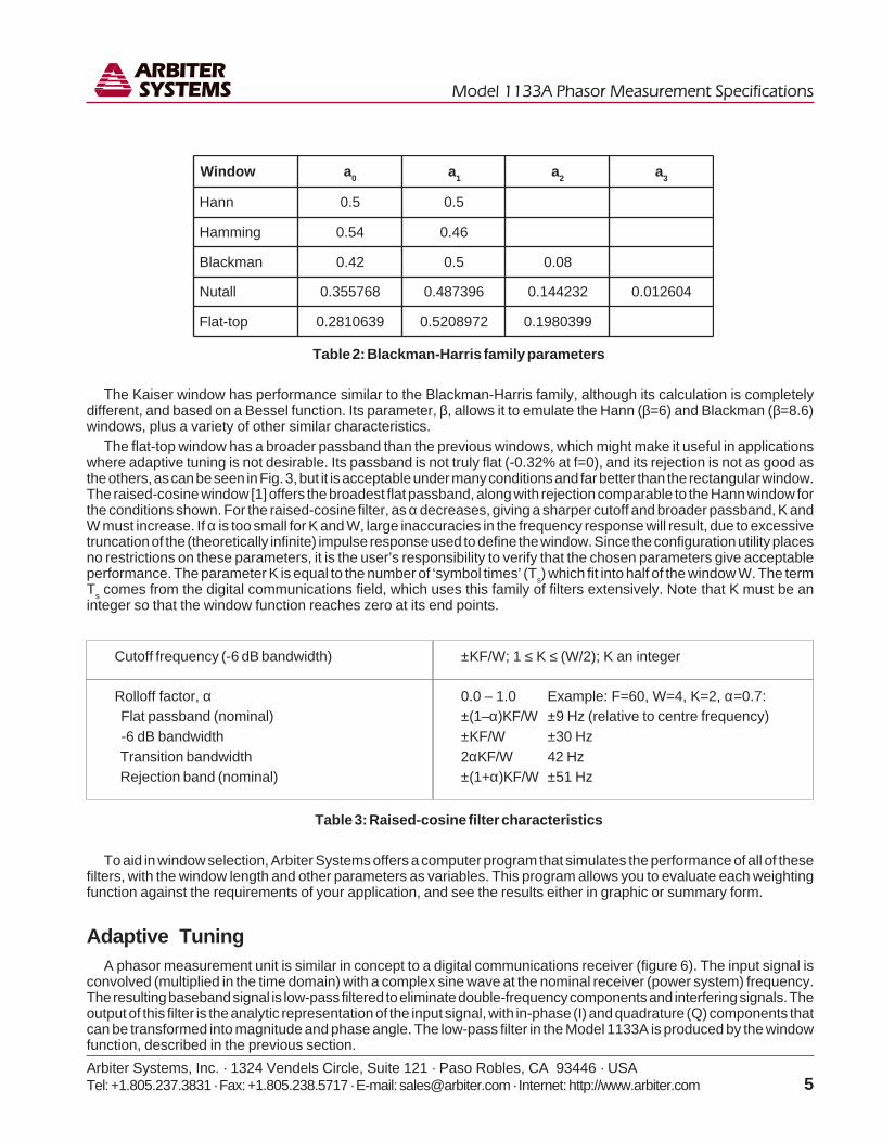
Table 2: Blackman-Harris family parameters

The Kaiser window has performance similar to the Blackman-Harris family, although its calculation is completelydifferent, and based on a Bessel function. Its parameter, β, allows it to emulate the Hann (β=6) and Blackman (β=8.6)windows, plus a variety of other similar characteristics.

The flat-top window has a broader passband than the previous windows, which might make it useful in applicationswhere adaptive tuning is not desirable. Its passband is not truly flat (-0.32% at f=0), and its rejection is not as good asthe others, as can be seen in Fig. 3, but it is acceptable under many conditions and far better than the rectangular window.The raised-cosine window [1] offers the broadest flat passband, along with rejection comparable to the Hann window forthe conditions shown. For the raised-cosine filter, as α decreases, giving a sharper cutoff and broader passband, K andW must increase. If α is too small for K and W, large inaccuracies in the frequency response will result, due to excessivetruncation of the (theoretically infinite) impulse response used to define the window. Since the configuration utility placesno restrictions on these parameters, it is the user’s responsibility to verify that the chosen parameters give acceptableperformance. The parameter K is equal to the number of ‘symbol times’ (T

s) which fit into half of the window W. The term

Ts comes from the digital communications field, which uses this family of filters extensively. Note that K must be an

integer so that the window function reaches zero at its end points.

Cutoff frequency (-6 dB bandwidth)

Rolloff factor, α Flat passband (nominal) -6 dB bandwidth Transition bandwidth Rejection band (nominal)

0.0 – 1.0 Example: F=60, W=4, K=2, α=0.7:±(1–α)KF/W ±9 Hz (relative to centre frequency)±KF/W ±30 Hz2αKF/W 42 Hz±(1+α)KF/W ±51 Hz

±KF/W; 1 ≤ K ≤ (W/2); K an integer

Table 3: Raised-cosine filter characteristics

To aid in window selection, Arbiter Systems offers a computer program that simulates the performance of all of thesefilters, with the window length and other parameters as variables. This program allows you to evaluate each weightingfunction against the requirements of your application, and see the results either in graphic or summary form.

Adaptive TuningA phasor measurement unit is similar in concept to a digital communications receiver (figure 6). The input signal is

convolved (multiplied in the time domain) with a complex sine wave at the nominal receiver (power system) frequency.The resulting baseband signal is low-pass filtered to eliminate double-frequency components and interfering signals. Theoutput of this filter is the analytic representation of the input signal, with in-phase (I) and quadrature (Q) components thatcan be transformed into magnitude and phase angle. The low-pass filter in the Model 1133A is produced by the windowfunction, described in the previous section.



6

As with a communications receiver, when the input signal moves away from the nominal receiver frequency, theresulting signal is attenuated by the filter frequency response. While filters can be designed to minimise attenuation overa certain bandwidth, there is still rolloff outside this band, and these filters may not have optimum characteristics for allapplications.

Rolloff effects can be reduced (practicallyeliminated) by continuously adjusting the receivercentre frequency to track the incoming signal (adaptivetuning), thereby keeping the convolver output in thecentre of the receiver passband as the input frequencychanges. However, this introduces the possibilitythat the frequency could mis-tune enough to preventproper operation. For an effective and reliable adaptive-tuning algorithm, we must address this possibility.

In the Model 1133A, the PMU centre frequency(when adaptive tuning is enabled) is set by thefrequency measured with the Model 1133A’s multi-purpose frequency-transducer function. Thismeasurement is made by determining w=∆φ/∆t ofV1, the positive-sequence voltage. This measurement has sufficient bandwidth that the signal will never get ‘lost.’Combined with a limit of ±2, 5, or 10 Hz maximum tuning range, errors due to rolloff can be eliminated while ensuringthat the algorithm never ‘loses’ the signal. As an additional ‘sanity check,’ the PMU magnitude results are cross-checkedagainst the broadband rms results from the 1133A’s multi-purpose transducer function, and adaptive tuning is disabledif the error exceeds a preset limit.

Adaptive tuning cannot be perfect, and it is worthwhile to consider the effects of slight mistuning on the PMU response.The effect on magnitude response is quite straightforward. Any errors are due to the very same filter rolloff that startedthe discussion. However, most filters are quite insensitive to mistuning near their centre frequency with respect tomagnitude response. Frequency offsets are random, caused by noise, and are generally much less than 0.01 Hz. Sincethe smallest 6 dB bandwidth possible with the window functions in the Model 1133A is approximately 5 Hz, it can be shownthat frequency noise will have a negligible effect – usually much less than 0.01%. Phase-angle accuracy is even lessdependent on frequency offsets, being totally insensitive to the centre frequency. Measured phase angle for any centrefrequency and signal frequency combination are identical, provided that the output of the low-pass filter is far enoughabove the noise floor.

Low-pass rejection, due to the window function, also must be considered since the double-frequency (image) productof the convolution process will alias into the passband (for any R ≤ 2F), and so must be rejected. Note that this is alsotrue if the frequency is at nominal, but most windows, even the rectangular window, have near-infinite rejection notchesin the vicinity of the harmonics of F/W (e.g., starting with N = 2…4 for the Blackman-Harris family). Rejection shouldbe at least 40 dB, and 60 dB is better, at 2F plus or minus expected frequency offsets. Indeed, this is one of the majorlimitations of first-generation PMUs. Off-nominal frequency signals aliased into the passband due to the limited rejectionof the one-cycle rectangular window (figure 3), causing significant errors [1].

In summary, adaptive tuning allows relatively-narrow estimator bandwidths, to provide anti-aliasing and rejection ofout-of-band signals, while still providing excellent accuracy measuring the magnitude and phase of the power-systemsignal. This is particularly useful for lower phasor reporting rates, below R = F/2 per second.

Synchronisation and ADC ResolutionInput sampling in the Model 1133A is performed using a time-multiplexed 14-bit A/D converter, synchronised to UTC

via the Global Positioning System to within one microsecond anywhere on earth (see figure 1). There has been somediscussion about the A/D conversion process as it relates to phasor estimation, particularly with respect tosynchronisation and resolution. Opinions have been expressed as fact, without a full appreciation of the nuances involvedin the design of sampled data systems. This has led to incorrect or oversimplified generalisations and misunderstandings.

Synchrophasors can be estimated in a number of ways. Contrary to common belief, there is no absolute requirementfor synchronised data samples or a particular ADC resolution in order to meet the requirements of the IEEEsynchrophasor standards. What is required by these standards is that the measurement (phasor estimate) be within



specified limits (±1% total vector error) at the reporting times specified. Phasors could be measured with a free-runningsample clock, provided some means is provided to determine the relationship between the ADC clock and UTC, and totransform the output so as to match the specified reporting times. While this is possible, it is not trivial, and we are notaware of any commercial implementations using this approach. Nevertheless, such an implementation properly doneshould give results which are equivalent (in the steady state, for which the standards apply, other factors being equal)to implementations using synchronised sampling. Note that this is not simply time-tagging the results. The IEEEstandards require that the phasor estimates be made at prescribed points in time, not simply tagged with the time theywere made. This requirement is intended to maximise compatibility between PMUs from different makers.

There is also no requirement for input sampling to be time-aligned with e.g. 1PPS-UTC. The reported results mustbe aligned – but this is an important difference. It is in fact impossible to sample a signal ‘exactly’ at the time of occurrenceof 1PPS-UTC, or at any other specific point in time. It is also unnecessary. If the sampling time is offset, then either(a) the amount of offset must be small enough so as not to compromise performance; in other words, the PMU mustmeet the 1% TVE requirement without correction for the offset; or (b) the PMU must compensate for the sampling offset.The standards contemplate this and allow for it (indeed they require it). Actually, one good method to compensate foranalog anti-alias filter delay is to intentionally delay the sampling clock by an equivalent amount.

There is also no requirement for a specific ADC resolution. There is a widespread misconception that performanceis limited in a fundamental way by the number of bits in the ADC. While there are several ADC parameters that can placefundamental limitations on performance – linearity, noise and gain stability for example – resolution is not one of them,at least not in itself.

For example, many modern systems (including some PMUs) use ‘sigma-delta’ A/D converters. Engineers often viewthese in terms of the number of rated output bits, commonly 16 to 24. We do not pay much attention to the fact that theseare really one-bit A/D converters, integrated with a digital filter which provides the enhanced output resolution.

The keys to understanding this seeming paradox are processing gain and noise shaping. A one-bit converter hasa theoretical signal-to-noise ratio of 1.76 dB for a full-scale signal. This might seem hardly useful for anything. However,if this converter is made to operate at a rate much higher than the measurement bandwidth, then the noise, spread overthe entire Nyquist bandwidth of dc to one-half of the sampling frequency, is reduced greatly by filtering since most ofit is outside the bandwidth of the filter. For example, a one-bit converter operating at one million samples per second (1MSPS) and used with a PMU having a 60 Hz measurement bandwidth could deliver a S/N ratio of about 41 dB – adequate(barely) to meet the 1% TVE requirement. The ratio of 60 Hz to 500 kHz (the Nyquist bandwidth), which is 8333 or 39.2dB, is called processing gain. The processing gain is greater for narrower measurement bandwidths, and for highersampling rates. In general, a converter having fewer bits and a higher sampling rate can provide performance equivalentto a converter with more bits and a lower sampling rate. It depends on the other parameters of the ADC, primarily linearityand noise, and on the use of the proper DSP algorithms. Engineers who design sampled-data systems understand andmake these tradeoffs routinely.

The preceding discussion presumes that the sampling noise is distributed evenly across the entire frequency bandfrom dc to the Nyquist limit. (For quantization noise in an ADC, this is true if the noise is not correlated to the input signal.This is a whole different subject, but the noise is mostly non-correlated if the input signal is large relative to ADCresolution, and/or the ratio of sampling to signal frequency is large. Correlated ‘noise’ produces harmonics andintermodulation products.) Consider what would happen, however, if the noise could be ‘shaped’ in the frequency domainso that more of it was outside the desired measurement bandwidth. If we could shape the noise spectrum, moving thequantization noise away from the desired signal, then the processing gain could be greater than simply the ratio of thebandwidths. This can in fact be done, by including the ADC inside a feedback loop having one or more integrators. Theintegrators reduce the amount of noise at low frequencies, at the expense of increasing it at high frequencies. Note thatthe total noise is always the same, and there is no ‘free lunch’ – all we are doing is moving the noise to a higher frequency,where it is attenuated by subsequent low-pass filtering. This process is called noise shaping, and is what makes itpossible to achieve signal-to-noise ratios of 100 dB or better with what is basically a one-bit converter.

Conclusion: there is no simple relationship between synchronisation method, ADC resolution, and synchrophasormeasurement performance. There is a relationship, of course, but not a simple one. We believe that the processimplemented in the Model 1133A is a good one, with respect to cost/performance tradeoffs, but we recognise that thereare many other ways to solve this problem. The manufacturer’s job in building a PMU is to understand the varioustradeoffs involved and select an implementation which optimises performance while meeting cost and reliabilityobjectives.



8

References[1] J. A. de la O Serna and K. E. Martin, “Improving Phasor Measurements Under Power System Oscillations,” IEEE

Trans. Power Sys., Vol. 18, No. 1, Feb. 2003.[2] IEEE Standard C37.118-2005, “Synchrophasors for Power Systems.”[3] A. H. Nutall, “Some Windows with Very Good Sidelobe Behavior,” IEEE Trans. Acoustics, Speech and Signal

Processing, Vol. ASSP-29, No. 1, Feb. 1981.[4] F. J. Harris, “On the Use of Windows for Harmonic Analysis with the Discrete Fourier Transform,” Proc. IEEE,

Vol. 66, No. 1, Jan. 1978.

PD0040400

model 1133a phasor measurement specifications 1133a phasor measurement specifications arbiter...

Documents