model-based geostatistics - leg-ufprverao2007:pdf:... · this is page i printer: opaque this...
TRANSCRIPT

This is page iPrinter: Opaque this
Model-based Geostatistics
Peter J. Diggle and Paulo J. Ribeiro Jr.
May 22, 2006
�2006 SPRINGER SCIENCE+BUSINESS MEDIA, LLC.
All rights reserved. No part of this work may be reproduced in any form withoutthe written permission of SPRINGER SCIENCE+BUSINESS MEDIA, LLC.

ii
Peter J. DiggleDepartment of Mathematics and StatisticsLancaster University, Lancaster, UKLA1 [email protected]
Paulo J. Ribeiro JrDepartamento de EstatısticaUniversidade Federal do ParanaC.P. 19.081Curitiba, Parana, [email protected]

This is page iiiPrinter: Opaque this
Preface
Geostatistics refers to the sub-branch of spatial statistics in which the dataconsist of a finite sample of measured values relating to an underlying spa-tially continuous phenomenon. Examples include: heights above sea-level in atopographical survey; pollution measurements from a finite network of monitor-ing stations; determinations of soil properties from core samples; insect countsfrom traps at selected locations. The subject has an interesting history. Orig-inally, the term geostatistics was coined by Georges Matheron and colleaguesat Fontainebleau, France, to describe their work addressing problems of spatialprediction arising in the mining industry. See, for example, Matheron (1963,1971). The ideas of the Fontainebleau school were developed largely indepen-dently of the mainstream of spatial statistics, with a distinctive terminology andstyle which tended to conceal the strong connections with parallel developmentsin spatial statistics. These parallel developments included work by Kolmogorov(1941), Matern (1960, reprinted as Matern, 1986), Whittle (1954, 1962, 1963),Bartlett (1964, 1967) and others. For example, the core geostatistical methodknown as simple kriging is equivalent to minimum mean square error predictionunder a linear Gaussian model with known parameter values. Papers by Wat-son (1971,1972) and the book by Ripley (1981) made this connection explicit.Cressie (1993) considered geostatistics to be one of three main branches of spa-tial statistics, the others being discrete spatial variation (covering distributionson lattices and Markov random fields) and spatial point processes. Geostatisti-cal methods are now used in many areas of application, far beyond the miningcontext in which they were originally developed.
Despite this apparent integration with spatial statistics, much geostatisticalpractice still reflects its independent origins, and from a mainstream statisti-cal perspective this has some undesirable consequences. In particular, explicit

iv
stochastic models are not always declared and ad hoc methods of inference areoften used, rather than the likelihood-based methods of inference which arecentral to modern statistics. The potential advantages of using likelihood-basedmethods of inference are two-fold: they generally lead to more efficient estima-tion of unknown model parameters; and they allow for the proper assessmentof the uncertainty in spatial predictions, including an allowance for the effectsof uncertainty in the estimation of model parameters.
Diggle, Tawn & Moyeed (1998) coined the phrase model-based geostatistics
to describe an approach to geostatistical problems based on the application offormal statistical methods under an explicitly assumed stochastic model. Thisbook takes the same point of view.
We aim to produce an applied statistical counterpart to Stein (1999), whogives a rigorous mathematical theory of kriging. Our intended readership in-cludes postgraduate statistics students and scientific researchers whose workinvolves the analysis of geostatistical data. The necessary statistical backgroundis summarised in an Appendix, and we give suggestions of further backgroundreading for readers meeting this material for the first time.
Throughout the book, we illustrate the statistical methods by applyingthem in the analysis of real data-sets. Most of the data-sets which we useare publically available and can be obtained from the book’s web-page,http://www.maths.lancs.ac.uk/∼diggle/mbg.
Most of the book’s chapters end with a section on computation, in which weshow how the R software (R Development Core Team 2005) and contributedpackages geoR and geoRglm can be used to implement the geostatistical meth-ods described in the corresponding chapters. This software is freely availablefrom the R Project web-page (http://www.r-project.org).
The first two chapters of the book provide an introduction and overview.Chapters 3 and 4 then describe geostatistical models whilst chapters 5 to 8 coverassociated methods of inference. The material is mostly presented for univariateproblems, i.e. those for which the measured response at any location consists of asingle value, but Chapter 3 includes a discussion of some multivariate extensionsto geostatistical models and associated statistical methods.
The connections between classical and model-based gostatistics are closestwhen, in our terms, the assumed model is the linear Gaussian model. Readerswho wish to confine their attention to this class of models on a first readingmay skip Sections 3.11, 3.12, Chapter 4, Sections 5.5, 7.5, 7.6 and Chapter 8.
Many friends and colleagues have helped us in various ways: by improvingour understanding of geostatistical theory and methods; by working with us ona range of collaborative projects; by allowing us to use their data-sets; and byoffering constructive criticism of early drafts. We particularly wish to thank OleChristensen, with whom we have enjoyed many helpful discussions. Ole is alsothe lead author of the geoRglm package.
Peter J Diggle, Paulo J Ribeiro Jr, March 2006.

This is page vPrinter: Opaque this
Contents
1 Introduction 1
1.1 Motivating examples . . . . . . . . . . . . . . . . . . . . . . 11.2 Terminology and notation . . . . . . . . . . . . . . . . . . . 9
1.2.1 Support . . . . . . . . . . . . . . . . . . . . . . . . . 9
1.2.2 Multivariate responses and explanatory variables . . 101.2.3 Sampling design . . . . . . . . . . . . . . . . . . . . . 12
1.3 Scientific objectives . . . . . . . . . . . . . . . . . . . . . . . 121.4 Generalised linear geostatistical models . . . . . . . . . . . . 13
1.5 What is in this book? . . . . . . . . . . . . . . . . . . . . . . 151.5.1 Organisation of the book . . . . . . . . . . . . . . . . 161.5.2 Statistical pre-requisites . . . . . . . . . . . . . . . . 17
1.6 Computation . . . . . . . . . . . . . . . . . . . . . . . . . . . 17
1.6.1 Elevation data . . . . . . . . . . . . . . . . . . . . . . 171.6.2 More on the geodata object . . . . . . . . . . . . . . 201.6.3 Rongelap data . . . . . . . . . . . . . . . . . . . . . . 22
1.6.4 The Gambia malaria data . . . . . . . . . . . . . . . 241.6.5 The soil data . . . . . . . . . . . . . . . . . . . . . . 24
1.7 Exercises . . . . . . . . . . . . . . . . . . . . . . . . . . . . . 26
2 An overview of model-based geostatistics 27
2.1 Design . . . . . . . . . . . . . . . . . . . . . . . . . . . . . . 27
2.2 Model formulation . . . . . . . . . . . . . . . . . . . . . . . . 282.3 Exploratory data analysis . . . . . . . . . . . . . . . . . . . 30
2.3.1 Non-spatial exploratory analysis . . . . . . . . . . . . 30
2.3.2 Spatial exploratory analysis . . . . . . . . . . . . . . 31

vi Contents
2.4 The distinction between parameter estimation and spatialprediction . . . . . . . . . . . . . . . . . . . . . . . . . . . . 35
2.5 Parameter estimation . . . . . . . . . . . . . . . . . . . . . . 362.6 Spatial prediction . . . . . . . . . . . . . . . . . . . . . . . . 372.7 Definitions of distance . . . . . . . . . . . . . . . . . . . . . 392.8 Computation . . . . . . . . . . . . . . . . . . . . . . . . . . . 402.9 Exercises . . . . . . . . . . . . . . . . . . . . . . . . . . . . . 44
3 Gaussian models for geostatistical data 46
3.1 Covariance functions and the variogram . . . . . . . . . . . . 463.2 Regularisation . . . . . . . . . . . . . . . . . . . . . . . . . . 483.3 Continuity and differentiability of stochastic processes . . . 493.4 Families of covariance functions and their properties . . . . . 51
3.4.1 The Matern family . . . . . . . . . . . . . . . . . . . 513.4.2 The powered exponential family . . . . . . . . . . . . 523.4.3 Other families . . . . . . . . . . . . . . . . . . . . . . 55
3.5 The nugget effect . . . . . . . . . . . . . . . . . . . . . . . . 563.6 Spatial trends . . . . . . . . . . . . . . . . . . . . . . . . . . 573.7 Directional effects . . . . . . . . . . . . . . . . . . . . . . . . 573.8 Transformed Gaussian models . . . . . . . . . . . . . . . . . 603.9 Intrinsic models . . . . . . . . . . . . . . . . . . . . . . . . . 623.10 Unconditional and conditional simulation . . . . . . . . . . . 663.11 Low-rank models . . . . . . . . . . . . . . . . . . . . . . . . 683.12 Multivariate models . . . . . . . . . . . . . . . . . . . . . . . 69
3.12.1 Cross-covariance, cross-correlation and cross-variogram 703.12.2 Bivariate signal and noise . . . . . . . . . . . . . . . 713.12.3 Some simple constructions . . . . . . . . . . . . . . . 72
3.13 Computation . . . . . . . . . . . . . . . . . . . . . . . . . . . 743.14 Exercises . . . . . . . . . . . . . . . . . . . . . . . . . . . . . 76
4 Generalized linear models for geostatistical data 78
4.1 General formulation . . . . . . . . . . . . . . . . . . . . . . . 784.2 The approximate covariance function and variogram . . . . . 804.3 Examples of generalised linear geostatistical models . . . . . 81
4.3.1 The Poisson log-linear model . . . . . . . . . . . . . . 814.3.2 The binomial logistic-linear model . . . . . . . . . . . 824.3.3 Spatial survival analysis . . . . . . . . . . . . . . . . 83
4.4 Point process models and geostatistics . . . . . . . . . . . . 854.4.1 Cox processes . . . . . . . . . . . . . . . . . . . . . . 864.4.2 Preferential sampling . . . . . . . . . . . . . . . . . . 88
4.5 Some examples of other model constructions . . . . . . . . . 924.5.1 Scan processes . . . . . . . . . . . . . . . . . . . . . . 924.5.2 Random sets . . . . . . . . . . . . . . . . . . . . . . . 93
4.6 Computation . . . . . . . . . . . . . . . . . . . . . . . . . . . 934.6.1 Simulating from the generalised linear model . . . . . 934.6.2 Preferential sampling . . . . . . . . . . . . . . . . . . 95
4.7 Exercises . . . . . . . . . . . . . . . . . . . . . . . . . . . . . 96

Contents vii
5 Classical parameter estimation 98
5.1 Trend estimation . . . . . . . . . . . . . . . . . . . . . . . . 995.2 Variograms . . . . . . . . . . . . . . . . . . . . . . . . . . . . 99
5.2.1 The theoretical variogram . . . . . . . . . . . . . . . 995.2.2 The empirical variogram . . . . . . . . . . . . . . . . 1015.2.3 Smoothing the empirical variogram . . . . . . . . . . 1015.2.4 Exploring directional effects . . . . . . . . . . . . . . 1035.2.5 The interplay between trend and covariance structure 104
5.3 Curve-fitting methods for estimating covariance structure . . 1065.3.1 Ordinary least squares . . . . . . . . . . . . . . . . . 1075.3.2 Weighted least squares . . . . . . . . . . . . . . . . . 1075.3.3 Comments on curve-fitting methods . . . . . . . . . . 109
5.4 Maximum likelihood estimation . . . . . . . . . . . . . . . . 1115.4.1 General ideas . . . . . . . . . . . . . . . . . . . . . . 1115.4.2 Gaussian models . . . . . . . . . . . . . . . . . . . . 1115.4.3 Profile likelihood . . . . . . . . . . . . . . . . . . . . 1135.4.4 Application to the surface elevation data. . . . . . . . 1135.4.5 Restricted maximum likelihood estimation for the
Gaussian linear model . . . . . . . . . . . . . . . . . 1155.4.6 Trans-Gaussian models . . . . . . . . . . . . . . . . . 1165.4.7 Analysis of Swiss rainfall data . . . . . . . . . . . . . 1175.4.8 Analysis of soil calcium data . . . . . . . . . . . . . . 120
5.5 Parameter estimation for generalized linear geostatisticalmodels . . . . . . . . . . . . . . . . . . . . . . . . . . . . . . 1225.5.1 Monte Carlo maximum likelihood . . . . . . . . . . . 1235.5.2 Hierarchical likelihood . . . . . . . . . . . . . . . . . 1245.5.3 Generalized estimating equations . . . . . . . . . . . 124
5.6 Computation . . . . . . . . . . . . . . . . . . . . . . . . . . . 1255.6.1 Variogram calculations . . . . . . . . . . . . . . . . . 1255.6.2 Parameter estimation . . . . . . . . . . . . . . . . . . 129
5.7 Exercises . . . . . . . . . . . . . . . . . . . . . . . . . . . . . 131
6 Spatial prediction 133
6.1 Minimum mean square error prediction . . . . . . . . . . . . 1336.2 Minimum mean square error prediction for the stationary
Gaussian model . . . . . . . . . . . . . . . . . . . . . . . . . 1356.2.1 Prediction of the signal at a point . . . . . . . . . . . 1356.2.2 Simple and ordinary kriging . . . . . . . . . . . . . . 1366.2.3 Prediction of linear targets . . . . . . . . . . . . . . . 1376.2.4 Prediction of non-linear targets . . . . . . . . . . . . 137
6.3 Prediction with a nugget effect . . . . . . . . . . . . . . . . 1386.4 What does kriging actually do to the data? . . . . . . . . . . 139
6.4.1 The prediction weights . . . . . . . . . . . . . . . . . 1406.4.2 Varying the correlation parameter . . . . . . . . . . . 1436.4.3 Varying the noise-to-signal ratio . . . . . . . . . . . . 145
6.5 Trans-Gaussian kriging . . . . . . . . . . . . . . . . . . . . . 1466.5.1 Analysis of Swiss rainfall data (continued) . . . . . . 148

viii Contents
6.6 Kriging with non-constant mean . . . . . . . . . . . . . . . . 1506.6.1 Analysis of soil calcium data (continued) . . . . . . . 150
6.7 Computation . . . . . . . . . . . . . . . . . . . . . . . . . . . 1506.8 Exercises . . . . . . . . . . . . . . . . . . . . . . . . . . . . . 154
7 Bayesian inference 156
7.1 The Bayesian paradigm: a unified treatment of estimation andprediction . . . . . . . . . . . . . . . . . . . . . . . . . . . . 1567.1.1 Prediction using plug-in estimates . . . . . . . . . . . 1567.1.2 Bayesian prediction . . . . . . . . . . . . . . . . . . . 1577.1.3 Obstacles to practical Bayesian prediction . . . . . . 159
7.2 Bayesian estimation and prediction for the Gaussian linearmodel . . . . . . . . . . . . . . . . . . . . . . . . . . . . . . . 1597.2.1 Estimation . . . . . . . . . . . . . . . . . . . . . . . . 1607.2.2 Prediction when correlation parameters are known . 1627.2.3 Uncertainty in the correlation parameters . . . . . . 1637.2.4 Prediction of targets which depend on both the signal
and the spatial trend . . . . . . . . . . . . . . . . . . 1647.3 Trans-Gaussian models . . . . . . . . . . . . . . . . . . . . . 1657.4 Case studies . . . . . . . . . . . . . . . . . . . . . . . . . . . 166
7.4.1 Surface elevations . . . . . . . . . . . . . . . . . . . . 1667.4.2 Analysis of Swiss rainfall data (continued) . . . . . . 167
7.5 Bayesian estimation and prediction for generalized lineargeostatistical models . . . . . . . . . . . . . . . . . . . . . . 1707.5.1 Markov Chain Monte Carlo . . . . . . . . . . . . . . 1717.5.2 Estimation . . . . . . . . . . . . . . . . . . . . . . . . 1727.5.3 Prediction . . . . . . . . . . . . . . . . . . . . . . . . 1757.5.4 Some possible improvements to the MCMC algorithm 176
7.6 Case studies in generalized linear geostatistical modelling . . 1787.6.1 Simulated data . . . . . . . . . . . . . . . . . . . . . 1787.6.2 Rongelap island . . . . . . . . . . . . . . . . . . . . . 1807.6.3 Childhood malaria in The Gambia . . . . . . . . . . 1847.6.4 Loa loa prevalence in equatorial Africa . . . . . . . . 187
7.7 Computation . . . . . . . . . . . . . . . . . . . . . . . . . . . 1927.7.1 Gaussian models . . . . . . . . . . . . . . . . . . . . 1927.7.2 Non-Gaussian Models . . . . . . . . . . . . . . . . . . 195
7.8 Exercises . . . . . . . . . . . . . . . . . . . . . . . . . . . . . 195
8 Geostatistical Design 198
8.1 Choosing the study region . . . . . . . . . . . . . . . . . . . 2008.2 Choosing the sample locations: uniform designs . . . . . . . 2008.3 Designing for efficient prediction . . . . . . . . . . . . . . . . 2028.4 Designing for efficient parameter estimation . . . . . . . . . 2038.5 A Bayesian design criterion . . . . . . . . . . . . . . . . . . . 204
8.5.1 Retrospective design . . . . . . . . . . . . . . . . . . 2058.5.2 Prospective design . . . . . . . . . . . . . . . . . . . 208
8.6 Exercises . . . . . . . . . . . . . . . . . . . . . . . . . . . . . 210

Contents ix
References 212
A Statistical background 221
A.1 Statistical models . . . . . . . . . . . . . . . . . . . . . . . . 221A.2 Classical inference . . . . . . . . . . . . . . . . . . . . . . . . 221A.3 Bayesian inference . . . . . . . . . . . . . . . . . . . . . . . . 223A.4 Prediction . . . . . . . . . . . . . . . . . . . . . . . . . . . . 224

This is page 27Printer: Opaque this
2
An overview of model-based geostatistics
The aim of this chapter is to provide a short overview of model-based geostatis-tics, using the elevation data of Example 1.1 to motivate the various stagesin the analysis. Although this example is very limited from a scientific point ofview, its simplicity makes it well-suited to the task in hand. Note, however, thatHandcock & Stein (1993) show how to construct a useful explanatory variablefor these data using a map of streams which run through the study-region.
2.1 Design
Statistical design is concerned with deciding what data to collect in order toaddress a question, or questions, of scientific interest. In this chapter, we shallassume that the scientific objective is to produce a map of surface elevationwithin a square study region whose side-length is 6.7 units, or 335 feet (≈ 102meters); we presume that this study-region has been chosen for good reason,either because it is of interest in its own right, or because it is representative ofsome wider spatial region.
In this simple setting, there are essentially only two design questions: at howmany locations should we measure the elevation? and where should we placethese locations within the study-region?
In practice, the answer to the first question is usually dictated by limitson the investigator’s time and/or any additional cost in converting each fieldsample into a measured value. For example, some kinds of measurements involveexpensive off-site laboratory assays whereas others, such as surface elevation,can be measured directly in the field. For whatever reason, the answer in thisexample is 52.

28 2. An overview of model-based geostatistics
For the second question, two obvious candidate designs are a completely ran-
dom design or a completely regular design. In the former, the locations xi forman independent random sample from the uniform distribution over the studyarea, i.e. a homogeneous planar Poisson process (Diggle, 2003, chapter 1). Inthe latter, the xi form a regular lattice pattern over the study-region. Classicalsampling theory (Cochran 1977) tends to emphasise the virtue of some form ofrandom sampling to ensure unbiased estimation of underlying population char-acteristics, whereas spatial sampling theory (Matern 1960) shows that undertypical modelling assumptions spatial properties are more efficiently estimatedby a regular design. A compromise, which the originators of the surface eleva-tion data appear to have adopted, is to use a design which is more regular thanthe completely random design but not as regular as a lattice.
Lattice designs are widely used in applications. The convenience of lat-tice designs for field-work is obvious, and provided there is no danger thatthe spacing of the lattice will match an underlying periodicity in the spatialphenomenon being studied, lattice designs are generally efficient for spatial pre-diction (Matern 1960). In practice, the rigidity and simplicity of a lattice designalso provide some protection against sub-conscious bias in the placing of the xi.Note in this context that, strictly, a regular lattice design should mean a latticewhose origin is located at random, to guard against any subjective bias. Thesoil data of Example 1.4 provide an example of a regular lattice design.
Even more common in some areas of application is the opportunistic design,whereby geostatistical data are collected and analysed using an existing networkof locations xi which may have been established for quite different purposes.Designs of this kind often arise in connection with environmental monitoring. Inthis context, individual recording stations may be set up to monitor pollutionlevels from particular industrial sources or in environmentally sensitive loca-tions, without any thought initially that the resulting data might be combinedin a single, spatial analysis. This immediately raises the possibility that the de-sign may be preferential, in the sense discussed in Section 1.2.3. Whether theyarise by intent or by accident, preferential designs run the risk that a standardgeostatistical analysis may produce misleading inferences about the underlyingcontinuous spatial variation.
2.2 Model formulation
We now consider model formulation – unusually before, rather than after, ex-ploratory data analysis. In practice, clean separation of these two stages is rare.However, in our experience it is useful to give some consideration to the kindof model which, in principle, will address the questions of interest before refin-ing the model through the usual iterative process of data analysis followed byreformulation of the model as appropriate.
For the surface elevation data, the scientific question is a simple one – how canwe use the measured elevations to construct our best guess (or, in more formallanguage, to predict) the underlying elevation surface throughout the study-

2.2. Model formulation 29
region? Hence, our model needs to include a real-valued, spatially continuousstochastic process, S(x) say, to represent the surface elevation as a functionof location, x. Depending on the nature of the terrain, we may want S(x) tobe continuous, differentiable or many-times differentiable. Depending on thenature of the measuring device, or the skill of its operator, we may also wantto allow for some discrepancy between the true surface elevation S(xi) andthe measured value Yi at the design location xi. The simplest statistical modelwhich meets these requirements is a stationary Gaussian model, which we definebelow. Later, we will discuss some of the many possible extensions of this modelwhich increase its flexibility.
We denote a set of geostatistical data in its simplest form, i.e. in the absenceof any explanatory variables, by (xi, yi) : i = 1, . . . , n where the xi are spatiallocations and yi is the measured value associated with the location xi. Theassumptions underlying the stationary Gaussian model are:
1. {S(x) : x ∈ IR2} is a Gaussian process with mean µ, variance σ2 =Var{S(x)} and correlation function ρ(u) = Corr{S(x), S(x′)}, where u =||x − x′|| and || · || denotes distance;
2. conditional on {S(x) : x ∈ IR2}, the yi are realisations of mutually in-dependent random variables Yi, Normally distributed with conditionalmeans E[Yi|S(·)] = S(xi) and conditional variances τ2.
The model can be defined equivalently as
Yi = S(xi) + Zi : i = 1, . . . , n
where {S(x) : x ∈ IR2} is defined by assumption 1 above and the Zi are mu-tually independent N(0, τ2) random variables. We favour the superficially morecomplicated conditional formulation for the joint distribution of the Yi giventhe signal, because it identifies the model explicitly as a special case of thegeneralized linear geostatistical model which we introduced in Section 1.4.
In order to define a legitimate model, the correlation function ρ(u) must bepositive-definite. This condition imposes non-obvious constraints so as to ensurethat, for any integer m, set of locations xi and real constants ai, the linearcombination
∑m
i=1aiS(xi) will have non-negative variance. In practice, this is
usually ensured by working within one of several standard classes of parametricmodel for ρ(u). We return to this question in Chapter 3. For the moment, wenote only that a flexible, two-parameter class of correlation functions due toMatern (1960) takes the form
ρ(u; φ, κ) = {2κ−1Γ(κ)}−1(u/φ)κKκ(u/φ) (2.1)
where Kκ(·) denotes the modified Bessel function of the second kind, of orderκ. The parameter φ > 0 determines the rate at which the correlation decays tozero with increasing u. The parameter κ > 0 is called the order of the Maternmodel, and determines the differentiability of the stochastic process S(x), in asense which we shall make precise in Chapter 3.
Our notation for ρ(u) presumes that u ≥ 0. However, the correlation functionof any stationary process must by symmetric in u, hence ρ(−u) = ρ(u).

30 2. An overview of model-based geostatistics
The stochastic variation in a physical quantity is not always well described bya Normal distribution. One of the simplest ways to extend the Gaussian modelis to assume that the model holds after applying a transformation to the originaldata. For positive-valued response variables, a useful class of transformations isthe Box-Cox family (Box & Cox 1964):
Y ∗ =
{
(Y λ − 1)/λ : λ 6= 0log Y : λ = 0
(2.2)
Another simple extension to the basic model is to allow a spatially varyingmean, for example by replacing the constant µ by a linear regression model forthe conditional expectation of Yi given S(xi), so defining a spatially varyingmean µ(x).
A third possibility is to allow S(x) to have non-stationary covariance struc-ture. Arguably, most spatial phenomena exhibit some form of non-stationarity,and the stationary Gaussian model should be seen only as a convenient ap-proximation to be judged on its usefulness rather than on its strict scientificprovenance.
2.3 Exploratory data analysis
Exploratory data analysis is an integral part of modern statistical practice, andgeostatistics is no exception. In the geostatistical setting, exploratory analysisis naturally oriented towards the preliminary investigation of spatial aspects ofthe data which are relevant to checking whether the assumptions made by anyprovisional model are approximately satisfied. However, non-spatial aspects canand should also be investigated.
2.3.1 Non-spatial exploratory analysis
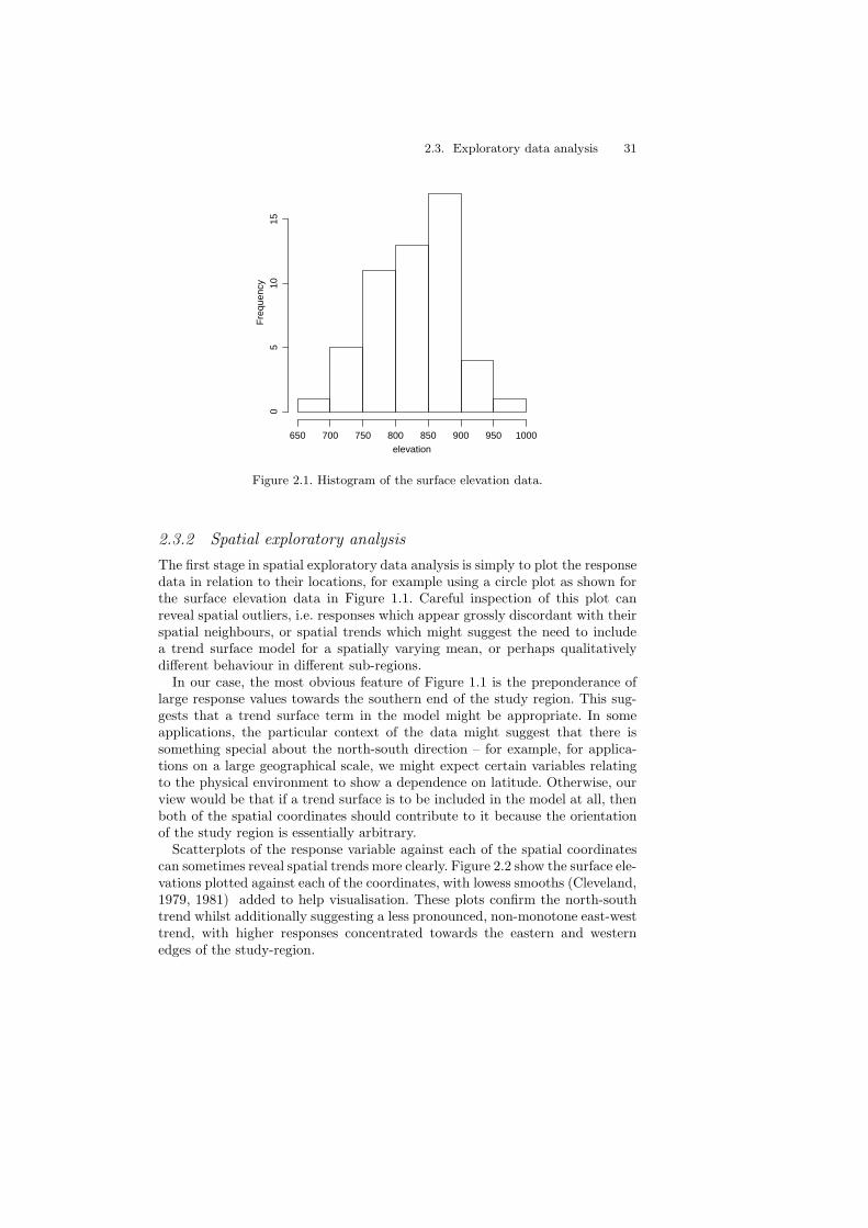
For the elevation data in Example 1.1 the 52 data values range from 690 to 960,with mean 827.1, median 830 and standard deviation 62. A histogram of the52 elevation values (Figure 2.1) indicates only mild asymmetry, and does notsuggest any obvious outliers. This adds some support to the use of a Gaussianmodel as an approximation for these data. Also, because geostatistical data are,at best, a correlated sample from a common underlying distribution, the shapeof their histogram will be less stable than that of an independent random sampleof the same size, and this limits the value of the histogram as a diagnostic fornon-Normality.
In general, an important part of exploratory analysis is to examine the re-lationship between the response and available covariates, as illustrated for thesoil data in Figure 1.7. For the current example, the only available covariatesto consider are the spatial coordinates themselves.
2.3. Exploratory data analysis 31
elevation
Fre
quen
cy
650 700 750 800 850 900 950 1000
05
1015
Figure 2.1. Histogram of the surface elevation data.
2.3.2 Spatial exploratory analysis
The first stage in spatial exploratory data analysis is simply to plot the responsedata in relation to their locations, for example using a circle plot as shown forthe surface elevation data in Figure 1.1. Careful inspection of this plot canreveal spatial outliers, i.e. responses which appear grossly discordant with theirspatial neighbours, or spatial trends which might suggest the need to includea trend surface model for a spatially varying mean, or perhaps qualitativelydifferent behaviour in different sub-regions.
In our case, the most obvious feature of Figure 1.1 is the preponderance oflarge response values towards the southern end of the study region. This sug-gests that a trend surface term in the model might be appropriate. In someapplications, the particular context of the data might suggest that there issomething special about the north-south direction – for example, for applica-tions on a large geographical scale, we might expect certain variables relatingto the physical environment to show a dependence on latitude. Otherwise, ourview would be that if a trend surface is to be included in the model at all, thenboth of the spatial coordinates should contribute to it because the orientationof the study region is essentially arbitrary.
Scatterplots of the response variable against each of the spatial coordinatescan sometimes reveal spatial trends more clearly. Figure 2.2 show the surface ele-vations plotted against each of the coordinates, with lowess smooths (Cleveland,1979, 1981) added to help visualisation. These plots confirm the north-southtrend whilst additionally suggesting a less pronounced, non-monotone east-westtrend, with higher responses concentrated towards the eastern and westernedges of the study-region.

32 2. An overview of model-based geostatistics
0 1 2 3 4 5 6
700
750
800
850
900
950
W−E
elev
atio
n da
ta
0 1 2 3 4 5 6
700
750
800
850
900
950
S−Nel
evat
ion
data
Figure 2.2. Elevation data against the coordinates.
When interpreting plots of this kind it can be difficult, especially whenanalysing small data-sets, to distinguish between a spatially varying meanresponse and correlated spatial variation about a constant mean. Strictly speak-ing, without independent replication the distinction between a deterministicfunction µ(x) and the realisation of a stochastic process S(x) is arbitrary. Op-erationally, we make the distinction by confining ourselves to “simple” functionsµ(x), for example low-order polynomial trend surfaces, using the correlationstructure of S(x) to account for more subtle patterns of spatial variation in theresponse. In Chapter 5 we shall use formal, likelihood-based methods to guideour choice of model for both mean and covariance structure. Less formally, weinterpret spatial effects which vary on a scale comparable to or greater thanthe dimensions of the study-region as variation in µ(x) and smaller-scale ef-fects as variation in S(x). This is in part a pragmatic strategy, since covariancefunctions which do not decay essentially to zero at distances shorter than thedimensions of the study region will be poorly identified, and in practice indis-tinguishable from spatial trends. Ideally, the model for the trend should alsohave a natural physical interpretation; for example, in an investigation of thedispersal of pollutants around a known source, it would be natural to modelµ(x) as a function of the distance, and possibly the orientation, of x relative tothe source.
To emphasise this point, the three panels of Figure 2.3 compare the originalFigure 1.1 with circle plots of residuals after fitting linear and quadratic trendsurface models by ordinary least squares. If we assume a constant spatial meanfor the surface elevations themselves, then the left-hand panel of Figure 2.3indicates that the elevations must be very strongly spatially correlated, to theextent that the correlation persists at distances beyond the scale of the studyregion. As noted above, fitting a model of this kind to the data would resultin poor identification of parameters describing the correlation structure. If, incontrast, we use a linear trend surface to describe a spatially varying mean,then the central panel of Figure 2.3 still suggests spatial correlation because
2.3. Exploratory data analysis 33
0 1 2 3 4 5 6
01
23
45
6
0 1 2 3 4 5 6
01
23
45
6
0 1 2 3 4 5 6
01
23
45
6
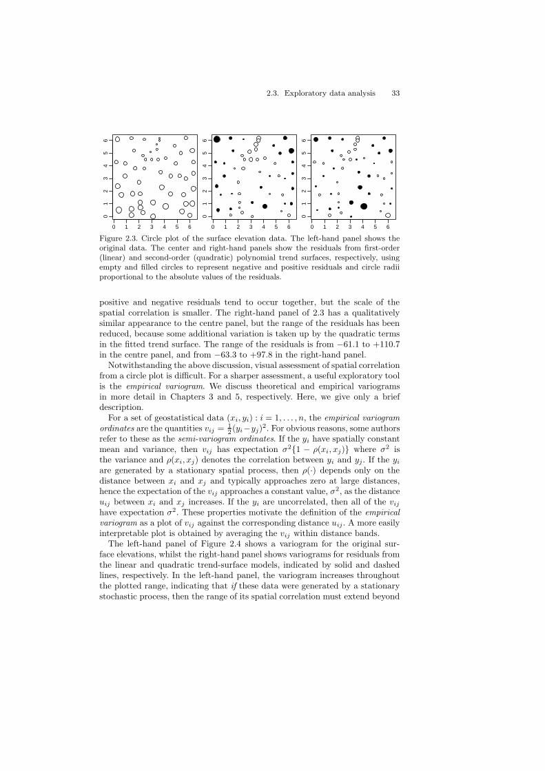
Figure 2.3. Circle plot of the surface elevation data. The left-hand panel shows theoriginal data. The center and right-hand panels show the residuals from first-order(linear) and second-order (quadratic) polynomial trend surfaces, respectively, usingempty and filled circles to represent negative and positive residuals and circle radiiproportional to the absolute values of the residuals.
positive and negative residuals tend to occur together, but the scale of thespatial correlation is smaller. The right-hand panel of 2.3 has a qualitativelysimilar appearance to the centre panel, but the range of the residuals has beenreduced, because some additional variation is taken up by the quadratic termsin the fitted trend surface. The range of the residuals is from −61.1 to +110.7in the centre panel, and from −63.3 to +97.8 in the right-hand panel.
Notwithstanding the above discussion, visual assessment of spatial correlationfrom a circle plot is difficult. For a sharper assessment, a useful exploratory toolis the empirical variogram. We discuss theoretical and empirical variogramsin more detail in Chapters 3 and 5, respectively. Here, we give only a briefdescription.
For a set of geostatistical data (xi, yi) : i = 1, . . . , n, the empirical variogram
ordinates are the quantities vij = 1
2(yi−yj)
2. For obvious reasons, some authorsrefer to these as the semi-variogram ordinates. If the yi have spatially constantmean and variance, then vij has expectation σ2{1 − ρ(xi, xj)} where σ2 isthe variance and ρ(xi, xj) denotes the correlation between yi and yj. If the yi
are generated by a stationary spatial process, then ρ(·) depends only on thedistance between xi and xj and typically approaches zero at large distances,hence the expectation of the vij approaches a constant value, σ2, as the distanceuij between xi and xj increases. If the yi are uncorrelated, then all of the vij
have expectation σ2. These properties motivate the definition of the empirical
variogram as a plot of vij against the corresponding distance uij . A more easilyinterpretable plot is obtained by averaging the vij within distance bands.
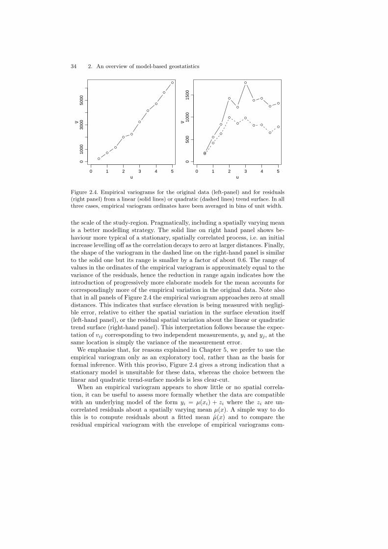
The left-hand panel of Figure 2.4 shows a variogram for the original sur-face elevations, whilst the right-hand panel shows variograms for residuals fromthe linear and quadratic trend-surface models, indicated by solid and dashedlines, respectively. In the left-hand panel, the variogram increases throughoutthe plotted range, indicating that if these data were generated by a stationarystochastic process, then the range of its spatial correlation must extend beyond
34 2. An overview of model-based geostatistics
0 1 2 3 4 5
010
0030
0050
00
u
v
0 1 2 3 4 5
050
010
0015
00
uv
Figure 2.4. Empirical variograms for the original data (left-panel) and for residuals(right panel) from a linear (solid lines) or quadratic (dashed lines) trend surface. In allthree cases, empirical variogram ordinates have been averaged in bins of unit width.
the scale of the study-region. Pragmatically, including a spatially varying meanis a better modelling strategy. The solid line on right hand panel shows be-haviour more typical of a stationary, spatially correlated process, i.e. an initialincrease levelling off as the correlation decays to zero at larger distances. Finally,the shape of the variogram in the dashed line on the right-hand panel is similarto the solid one but its range is smaller by a factor of about 0.6. The range ofvalues in the ordinates of the empirical variogram is approximately equal to thevariance of the residuals, hence the reduction in range again indicates how theintroduction of progressively more elaborate models for the mean accounts forcorrespondingly more of the empirical variation in the original data. Note alsothat in all panels of Figure 2.4 the empirical variogram approaches zero at smalldistances. This indicates that surface elevation is being measured with negligi-ble error, relative to either the spatial variation in the surface elevation itself(left-hand panel), or the residual spatial variation about the linear or quadratictrend surface (right-hand panel). This interpretation follows because the expec-tation of vij corresponding to two independent measurements, yi and yj, at thesame location is simply the variance of the measurement error.
We emphasise that, for reasons explained in Chapter 5, we prefer to use theempirical variogram only as an exploratory tool, rather than as the basis forformal inference. With this proviso, Figure 2.4 gives a strong indication that astationary model is unsuitable for these data, whereas the choice between thelinear and quadratic trend-surface models is less clear-cut.
When an empirical variogram appears to show little or no spatial correla-tion, it can be useful to assess more formally whether the data are compatiblewith an underlying model of the form yi = µ(xi) + zi where the zi are un-correlated residuals about a spatially varying mean µ(x). A simple way to dothis is to compute residuals about a fitted mean µ(x) and to compare theresidual empirical variogram with the envelope of empirical variograms com-

2.4. The distinction between parameter estimation and spatial prediction 35
0 1 2 3 4 5
050
010
0015
0020
00
u
v
0 1 2 3 4 5
050
010
0015
00
uv
Figure 2.5. Monte Carlo envelopes for the variogram of ordinary least squares resid-uals of the surface elevation data after fitting linear (left-hand panel) or quadratic(right-hand panel) trend surface models.
puted from random permutations of the residuals, holding the correspondinglocations fixed. The left-hand panel of Figure 2.5 shows a variogram envelopeobtained from 99 independent random permutations of the residuals from alinear trend surface fitted to the surface elevations by ordinary least squares.This shows that the increasing trend in the empirical variogram is statisticallysignificant, confirming the presence of positive spatial correlation. The sametechnique applied to the residuals from the quadratic trend surface producesthe diagram shown as the right-hand panel of Figure 2.5. This again indicatessignificant spatial correlation, although the result is less clear-cut than before,as the empirical variogram ordinates at distances 0.5 and 1.0 fall much closerto the lower simulation envelope than they do in the left-hand panel.
2.4 The distinction between parameter estimation andspatial prediction
Before continuing with our illustrative analysis of the surface elevation data, wedigress to expand on the distinction between estimation and prediction.
Suppose that S(x) represents the level of air pollution at the location x,that we have observed (without error, in this hypothetical example) the valuesSi = S(xi) at a set of locations xi : i = 1, . . . , n forming a regular lattice over aspatial region of interest, A, and that we wish to learn about the average levelof pollution over the region A. An intuitively reasonable estimate is the samplemean,
S = n−1
n∑
i=1
Si. (2.3)

36 2. An overview of model-based geostatistics
What precision should we attach to this estimate?Suppose that S(x) has aconstant expectation, θ = E[S(x)] for any location x
in A. One possible interpretation of S is as an estimate of θ, in which case anappropriate measure of precision is the mean square error, E[(S − θ)2]. This isjust the variance of S, which we can calculate as
n−2
n∑
i=1
n∑
j=1
Cov(Si, Sj). (2.4)
For a typical geostatistical model, the correlation between any two Si and Sj
will be either zero or positive, and (2.4) will therefore be larger than the naiveexpression for the variance of a sample mean, σ2/n where σ2 = Var{S(x)}.
If we regard S as a predictor of the spatial average,
SA = |A|−1
∫
A
S(x)dx,
where |A| is the area of A, then the mean square prediction error is E[(S−SA)2].Noting that SA is a random variable, we write this as
E[(S − SA)2] = n−2
n∑
i=1
n∑
j=1
Cov(Si, Sj)
+ |A|−2
∫
A
∫
A
Cov{S(x), S(x′)}dxdx′
− 2(n|A|)−1
n∑
i=1
∫
A
Cov{S(x), S(xi)}dx. (2.5)
In particular, the combined effect of the second and third terms on the righthand side of (2.5) can easily be to make the mean square prediction error smallerthan the naive variance formula. For example, if we increase the sample size nby progressively decreasing the spacing of the lattice points xi, (2.5) approacheszero, whereas (2.4) does not.
2.5 Parameter estimation
For the stationary Gaussian model, the parameters to be estimated are themean µ and any additional parameters which define the covariance structureof the data. Typically, these include the signal variance σ2, the conditional ormeasurement error variance τ2 and one or more correlation function parametersφ.
In geostatistical practice, these parameters can be estimated in a number ofdifferent ways which we shall discuss in detail in Chapter 5. Our preferencehere is to use the method of maximum likelihood within the declared Gaussianmodel.
For the elevation data, if we assume a stationary Gaussian model with aMatern correlation function and a fixed value κ = 1.5, the maximum likelihood

2.6. Spatial prediction 37
estimates of the remaining parameters are µ = 848.3, σ2 = 3510.1, τ2 = 48.2and φ = 1.2.
However, our exploratory analysis suggested a model with a non-constantmean. Here, we assume a linear trend surface,
µ(x) = β0 + β1d1 + β2d2
where d1 and d2 are the north-south and east-west coordinates. In this casethe parameter estimates are β0 = 912.5, β1 = −5, β2 = −16.5, σ2 = 1693.1,τ2 = 34.9 and φ = 0.8. Note that because the trend surface accounts for someof the spatial variation, the estimate of σ2 is considerably smaller than for thestationary model, and similarly for the parameter φ which corresponds to therange of the spatial correlation. As anticipated, for either model the estimateof τ2 is much smaller than the estimate of σ2. The ratio of τ2 to σ2 is 0.014 forthe stationary model, and 0.021 for the linear trend surface model.
2.6 Spatial prediction
For prediction of the underlying, spatially continuous elevation surface we shallhere illustrate perhaps the simplest of all geostatistical methods: simple kriging.In our terms, simple kriging is minimum mean square error prediction under thestationary Gaussian model, but ignoring parameter uncertainty, i.e. estimatesof all model parameters are plugged into the prediction equations as if theywere the true parameter values. As discussed earlier, we do not claim that thisis a good model for the surface elevation data.
The minimum mean square error predictor, S(x) say, of S(x) at an arbitrarylocation x is the function of the data, y = (y1, . . . , yn), which minimises thequantity E[{S(x) − S(x)}2]. A standard result, which we discuss in Chapter 6,is that S(x) = E[S(x)|y]. For the stationary Gaussian process, this conditionalexpectation is a linear function of the yi, namely
S(x) = µ +n
∑
i=1
wi(x)(yi − µ) (2.6)
where the wi(x) are explicit functions of the covariance parameters σ2, τ2 andφ.
The top-left panel of Figure 2.6 gives the result of applying (2.6) to thesurface elevation data, using as values for the model parameters the maximumlikelihood estimates reported in Section 2.5, whilst the bottom-left panel showsthe corresponding prediction standard errors, SE(x) =
√Var{S(x)|y}. The
predictions follow the general trend of the observed elevations whilst smoothingout local irregularities. The prediction variances are generally small at locationsclose to the sampling locations, because τ 2 is relatively small; had we used thevalue τ2 = 0 the prediction standard error would have been exactly zero at eachsampling location and the predicted surface S(x) would have interpolated theobserved responses yi.
38 2. An overview of model-based geostatistics
0 1 2 3 4 5 6
01
23
45
6
0 1 2 3 4 5 60
12
34
56
0 1 2 3 4 5 6
01
23
45
6 + + + + +
+ +++ +
++
+ +
++ + + +
+ +
+
+ ++
+ ++
++
+ +
+ + +
+ +
+ +
+ +
+ +
+
++
+
++
+
+
+
0 1 2 3 4 5 6
01
23
45
6 + + + + +
+ +++ +
++
+ +
++ + + +
+ +
+
+ ++
+ ++
++
+ +
+ + +
+ +
+ +
+ +
+ +
+
++
+
++
+
+
+
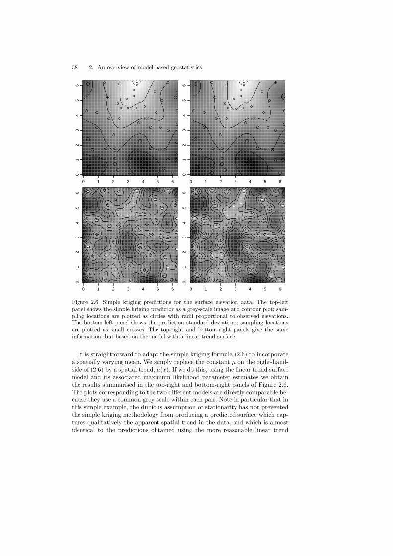
Figure 2.6. Simple kriging predictions for the surface elevation data. The top-leftpanel shows the simple kriging predictor as a grey-scale image and contour plot; sam-pling locations are plotted as circles with radii proportional to observed elevations.The bottom-left panel shows the prediction standard deviations; sampling locationsare plotted as small crosses. The top-right and bottom-right panels give the sameinformation, but based on the model with a linear trend-surface.
It is straightforward to adapt the simple kriging formula (2.6) to incorporatea spatially varying mean. We simply replace the constant µ on the right-hand-side of (2.6) by a spatial trend, µ(x). If we do this, using the linear trend surfacemodel and its associated maximum likelihood parameter estimates we obtainthe results summarised in the top-right and bottom-right panels of Figure 2.6.The plots corresponding to the two different models are directly comparable be-cause they use a common grey-scale within each pair. Note in particular that inthis simple example, the dubious assumption of stationarity has not preventedthe simple kriging methodology from producing a predicted surface which cap-tures qualitatively the apparent spatial trend in the data, and which is almostidentical to the predictions obtained using the more reasonable linear trend

2.7. Definitions of distance 39
surface model. The two models produce somewhat different prediction stan-dard errors; these range between 0 and 25.5 for the stationary model, between0 and 24.4 for the model with the linear trend surface and between 0 and 22.9for the model with the quadratic trend surface. The differences amongst thethree models are rather small. They are influenced by several different aspectsof the data and model, including the data-configuration and the estimated val-ues of the model parameters. In other applications, the choice of model mayhave a stronger impact on the predictive inferences we make from the data,even when this choice does not materially affect the point predictions of theunderlying surface S(x). Note also that the plug-in standard errors quoted heredo not account for parameter uncertainty.
2.7 Definitions of distance
A fundamental stage in any geostatistical analysis is to define the metric for cal-culating the distance between any two locations. By default, we use the standardplanar Euclidean distance, i.e. the“straight-line distance”between two locationsin IR2. Non-Euclidean metrics may be more appropriate for some applications.For example, Rathbun (1998) discusses the measurement of distance betweenpoints in an estuarine environment where, arguably, two locations which areclose in the Euclidean metric but separated by dry land should not be consid-ered as near neighbours. It is not difficult to think of other settings where naturalbarriers to communication might lead the investigator to question whether it isreasonable to model spatial correlation in terms of straight-line distance.
Even when straight-line distance is an appropriate metric, if the study-regionis geographically extensive, distances computed between points on the earth’ssurface should strictly be great-circle distances, rather than straight-line dis-tances on a map projection. Using (θ, φ) to denote a location in degrees oflongitude and latitude, and treating the earth as a sphere of radius r = 6378kilometres, the great-circle distance between two locations is
r cos−1{sinφ1 sin φ2 + cosφ1 cosφ2 cos(θ1 − θ2)}.
Section 3.2 of Waller & Gotway (2004) gives a nice discussion of this issuefrom a statistical perspective. Banerjee (2005) examines the effect of distancecomputations on geostatistical analysis and concludes that the choice of metricmay influence the resulting inferences, both for parameter estimation and forprediction. Note in particular that degrees of latitude and longitude representapproximately equal distances only close to the equator.
Distances calculations are especially relevant to modelling spatial correlation,hence parameters which define the correlation structure are particularly sensi-tive to the choice of metric. Furthermore, the Euclidean metric plays an integralpart in determining valid classes of correlation functions using Bochner’s the-orem (Stein 1999). Our geoR software implementation only calculates planarEuclidean distances.

40 2. An overview of model-based geostatistics
2.8 Computation
The non-spatial exploratory analysis of the surface elevation data reported inthis chapter uses only built-in R functions as follows.
> with(elevation, hist(data, main = "", xlab = "elevation"))
> with(elevation, plot(coords[, 1], data, xlab = "W-E",
+ ylab = "elevation data", pch = 20, cex = 0.7))
> lines(lowess(elevation$data ~ elevation$coords[, 1]))
> with(elevation, plot(coords[, 2], data, xlab = "S-N",
+ ylab = "elevation data", pch = 20, cex = 0.7))
> lines(with(elevation, lowess(data ~ coords[, 2])))
To produce circle plots of the residual data we use the geoR functionpoints.geodata(), which is invoked automatically when a geodata object ispassed as an argument to the built-in function points(), as indicated below.The argument trend defines a linear model on the covariates from which theresiduals are extracted for plotting. The values "1st" and "2nd" passed to theargument trend are aliases to indicate first and second degree polynomials onthe coordinates. More details and other options to specify the trend are dis-cussed later in this Section and in the documentation for trend.spatial().Setting abs=T instructs the function to draw the circles with radii proportionalto the absolute values of the residuals.
> points(elevation, cex.max = 2.5)
> points(elevation, trend = "1st", pt.div = 2, abs = T,
+ cex.max = 2.5)
> points(elevation, trend = "2nd", pt.div = 2, abs = T,
+ cex.max = 2.5)
To calculate and plot the empirical variograms shown in Figure 2.4 for theoriginal data and for the residuals, we use variog(). The argument uvec definesthe classes of distance used when computing the empirical variogram, whilstplot() recognises that its argument is a variogram object, and automaticallyinvokes plot.variogram(). The argument trend is used to indicate that thevariogram should be calculated from the residuals about a fitted trend surface.
> plot(variog(elevation, uvec = seq(0, 5, by = 0.5)),
+ type = "b")
> res1.v <- variog(elevation, trend = "1st", uvec = seq(0,
+ 5, by = 0.5))
> plot(res1.v, type = "b")
> res2.v <- variog(elevation, trend = "2nd", uvec = seq(0,
+ 5, by = 0.5))
> lines(res2.v, type = "b", lty = 2)
To obtain the residual variogram and simulation envelopes under random per-mutation of the residuals, as shown in Figure 2.5, we proceed as in the followingexample. By default, the function uses 99 simulations, but this can be changedusing the optional argument nsim.

2.8. Computation 41
> set.seed(231)
> mc1 <- variog.mc.env(elevation, obj = res1.v)
> plot(res1.v, env = mc1, xlab = "u")
> mc2 <- variog.mc.env(elevation, obj = res2.v)
> plot(res2.v, env = mc2, xlab = "u")
To obtain maximum likelihood estimates of the Gaussian model, with or withouta trend term, we use the geoR function likfit(). Because this function usesa numerical maximisation procedure, the user needs to provide initial valuesfor the covariance parameters, using the argument ini. In this example we usethe default value 0 for the parameter τ2, in which case ini specifies initialvalues for the parameters σ2 and φ. Initial values are not required for the meanparameters.
> ml0 <- likfit(elevation, ini = c(3000, 2), cov.model = "matern",
+ kappa = 1.5)
> ml0
likfit: estimated model parameters:
beta tausq sigmasq phi
" 848.317" " 48.157" "3510.096" " 1.198"
likfit: maximised log-likelihood = -242.1
> ml1 <- likfit(elevation, trend = "1st", ini = c(1300,
+ 2), cov.model = "matern", kappa = 1.5)
> ml1
likfit: estimated model parameters:
beta0 beta1 beta2 tausq sigmasq
" 912.4865" " -4.9904" " -16.4640" " 34.8953" "1693.1329"
phi
" 0.8061"
likfit: maximised log-likelihood = -240.1
To carry out the spatial interpolation using simple kriging we first define, andstore in the object locs, a grid of locations at which predictions of the valuesof the underlying surface are required. The function krige.control() thendefines the model to be used for the interpolation, which is carried out bykrige.conv(). In the example below, we first obtain predictions for the sta-tionary model, and then for the model with a linear trend on the coordinates.If required, the user can restrict the trend surface model, for example by spec-ifying a linear trend is the north-south direction. However, as a general rulewe prefer our inferences to be invariant to the particular choice of coordinateaxes, and would therefore fit both linear trend parameters or, more generally,full polynomial trend surfaces.
> locs <- pred_grid(c(0, 6.3), c(0, 6.3), by = 0.1)
> KC <- krige.control(type = "sk", obj.mod = ml0)

42 2. An overview of model-based geostatistics
> sk <- krige.conv(elevation, krige = KC, loc = locs)
> KCt <- krige.control(type = "sk", obj.mod = ml1, trend.d = "1st",
+ trend.l = "1st")
> skt <- krige.conv(elevation, krige = KCt, loc = locs)
Finally, we use a selection of built-in graphical functions to produce the mapsshown in Figure 2.6, using optional arguments to the graphical functions toensure that pairs of corresponding plots use the same grey-scale.
> pred.lim <- range(c(sk$pred, skt$pred))
> sd.lim <- range(sqrt(c(sk$kr, skt$kr)))
> image(sk, col = gray(seq(1, 0, l = 51)), zlim = pred.lim)
> contour(sk, add = T, nlev = 6)
> points(elevation, add = TRUE, cex.max = 2)
> image(skt, col = gray(seq(1, 0, l = 51)), zlim = pred.lim)
> contour(skt, add = T, nlev = 6)
> points(elevation, add = TRUE, cex.max = 2)
> image(sk, value = sqrt(sk$krige.var), col = gray(seq(1,
+ 0, l = 51)), zlim = sd.lim)
> contour(sk, value = sqrt(sk$krige.var), levels = seq(10,
+ 27, by = 2), add = T)
> points(elevation$coords, pch = "+")
> image(skt, value = sqrt(skt$krige.var), col = gray(seq(1,
+ 0, l = 51)), zlim = sd.lim)
> contour(skt, value = sqrt(skt$krige.var), levels = seq(10,
+ 27, by = 2), add = T)
> points(elevation$coords, pch = "+")
In geoR, covariates which define a linear model for the mean response can bespecified by passing additional arguments to plotting or model-fitting functions.In the examples above, we used trend="1st" or trend="2nd" to specify a lin-ear or quadratic trend surface. However, these are simply short-hand aliasesto formulae which define the corresponding linear models, and are providedfor users’ convenience. For example, the model formula trend=~coords[,1] +
coords[,2] would produce the same result as trend="1st". The trend argu-ment will also accept a matrix representing the design matrix of a general linearmodel, or the output of the trend definition function, trend.spatial(). Forexample, the call below to plot() can be used in order to inspect the dataafter taking out the linear effect of the north-south coordinate. By setting theargument trend=~coords[,2] the function fits a standard linear model on thiscovariate and uses the residuals to produce the plots shown in Figure 2.7, ratherthan plotting the original response data. Similarly, we could fit a quadratic func-tion on the x-coordinate by setting trend=~coords[,2] + poly(coords[,1],
degree=2). We invite the reader to experiment with different options for theargument trend and trend.spatial(). The procedure of taking out the effectof a covariate is sometimes called trend removal.
> plot(elevation, low = TRUE, trend = ~coords[, 2], qt.col = 1)

2.8. Computation 43
0 1 2 3 4 5 6
01
23
45
6
X Coord
Y C
oord
−50 0 50 100
01
23
45
6
residuals
Coo
rd Y
0 1 2 3 4 5 6
−50
050
100
Coord X
resi
dual
s
residuals
Fre
quen
cy
−50 0 50 100
02
46
810
12
Figure 2.7. Output of plot.geodata() when setting the argumenttrend=~coords[,2].
The trend argument can also be used to take account of covariates other thanfunctions of the coordinates. For example, the data set ca20 included in geoR
stores the calcium content from soil samples, as discussed in Example 1.4, to-gether with associated covariate information. Recall that in this example thestudy region is divided in three sub-regions with different histories of soil man-agement. The covariate area included in the data-set indicates for each datumthe sub-region in which it was collected. Figure 2.8 shows the exploratory plotfor the residuals after removing a separate mean for calcium content in eachsub-region. This diagram was produced using the following code.
> data(ca20)
> plot(ca20, trend = ~area, qt.col = 1)
The plotting functions in geoR also accept an optional argument lambda
which specifies the numerical value for the parameter of the Box-Cox family

44 2. An overview of model-based geostatistics
5000 5200 5400 5600 5800 6000
4800
5000
5200
5400
5600
5800
X Coord
Y C
oord
−20 −10 0 10 20
4800
5000
5200
5400
5600
5800
residuals
Coo
rd Y
5000 5200 5400 5600 5800 6000
−20
−10
010
20
Coord X
resi
dual
s
residuals
Fre
quen
cy
−30 −20 −10 0 10 20 30
010
2030
40
Figure 2.8. Exploratory plot for the ca20 data-set obtained when setting trend=~area.
of transformations, with default lambda=1 corresponding to no transformation.For example, the command
> plot(ca20, lambda = 0)
sets the Box-Cox transformation parameter to λ = 0, which will then produceplots using the logarithm of the original response variable.
2.9 Exercises
2.1. Investigate the R packages splancs or spatstat, both of which providefunctions for the analysis of spatial point pattern data. Use either of thesepackages to confirm (or not, as the case may be) that the design usedfor the surface elevation data is more regular than a completely randomdesign.

2.9. Exercises 45
2.2. Consider the following two models for a set of responses, Yi : i = 1, . . . , nassociated with a sequence of positions xi : i = 1, . . . , n along a one-dimensional spatial axis x.
(a) Yi = α + βxi + Zi, where α and β are parameters and the Zi aremutually independent with mean zero and variance σ2
Z .(b) Yi = A + Bxi + Zi where the Zi are as in (a) but A and B are now
random variables, independent of each other and of the Zi, each withmean zero and respective variances σ2
A and σ2
B .
For each of these models, find the mean and variance of Yi and the covari-ance between Yi and Yj for any j 6= i. Given a single realisation of eithermodel, would it be possible to distinguish between them?
2.3. Suppose that Y = (Y1, . . . , Yn) follows a multivariate Normal distributionwith E[Yi] = µ and Var{Yi} = σ2 and that the covariance matrix of Ycan be expressed as V = σ2R(φ). Write down the log-likelihood functionfor θ = (µ, σ2, φ) based on a single realisation of Y and obtain explicitexpressions for the maximum likelihood estimators of µ and σ2 when φis known. Discuss how you would use these expressions to find maximumlikelihood estimators numerically when φ is unknown.
2.4. Load the ca20 data-set with data(ca20). Check the data-set documen-tation with help(ca20). Perform an exploratory analysis of these data.Would you include a trend term in the model? Would you recommend adata transformation? Is there evidence of spatial correlation?
2.5. Load the Parana data with data(parana) and repeat Exercise 2.4.