model choice for phylogeographic inference using a large set of models

Acc

epte

d A

rtic

le

This article has been accepted for publication and undergone full peer review but has not been through the copyediting, typesetting, pagination and proofreading process, which may lead to differences between this version and the Version of Record. Please cite this article as doi: 10.1111/mec.12722 This article is protected by copyright. All rights reserved.

Received Date : 14-Aug-2013 Revised Date : 14-Feb-2014 Accepted Date : 25-Feb-2014 Article type : Original Article Model Choice for Phylogeographic Inference using a Large Set of Models

Running title: Model choice in Plethodon idahoensis.

Tara A. Pelletier1 and Bryan C. Carstens1*

1Department of Evolution, Ecology, and Organismal Biology, The Ohio State University. 318 W.

12th Avenue, Columbus, OH 43210-1293.

*Corresponding author: Bryan C. Carstens

email: [email protected]

Abstract

Model-based analyses are common in phylogeographic inference because they parameterize

processes such as population division, gene flow and expansion that are of interest to biologists.

Approximate Bayesian Computation is a model-based approach that can be customized to any

empirical system and used to calculate the relative posterior probability of several models,

provided that suitable models can be identified for comparison. The question of how to identify

suitable models is explored using data from Plethodon idahoensis, a salamander that inhabits the

North American inland northwest temperate rainforest. First, we conduct an ABC analysis using

Acc

epte

d A

rtic

le

This article is protected by copyright. All rights reserved.

five models suggested by previous research, calculate the relative posterior probabilities, and

find that a simple model of population isolation has the best fit to the data (PP = 0.70). In

contrast to this subjective choice of models to include in the analysis, we also specify models in a

more objective manner by simulating prior distributions for 143 models that included panmixia,

population isolation, change in effective population size, migration, and range expansion. We

then identify a smaller subset of models for comparison by generating an expectation of the

highest posterior probability that a false model is likely to achieve due to chance and calculate

the relative posterior probabilities of only those models that exceed this expected level. A model

that parameterized divergence with population expansion and gene flow in one direction, offered

the best fit to the P. idahoensis data (in contrast to an isolation only model from the first

analysis). Our investigation demonstrates that the determination of which models to include in

ABC model choice experiments is a vital component of model-based phylogeographic analysis.

Keywords: Plethodon idahoensis, Pacific Northwest, approximate Bayesian computation,

posterior predictive simulation, demographic model selection

Introduction

Model-based analyses have become a common component of phylogeographic inference because

they parameterize evolutionary processes that are of interest to biologists (Beaumont et al. 2010).

To conduct a model-based phylogeographic analysis, the choices available to researchers range

from full likelihood implementations of predefined models to approximate methods that allow

substantial customization of the model to the particulars of any empirical system. We prefer the

latter option because it allows researchers to evaluate multiple demographic models relevant to

their system, and to identify the model that offers the best fit to their data. In these cases, the

Acc

epte

d A

rtic

le


process of model selection can guide phylogeographic inference by identifying the evolutionary

processes (i.e., parameters) that have shaped the patterns of genetic variation (Carstens et al.

2013).

While model-based methods offer a number of benefits to phylogeographic investigations

(Knowles 2009), the question of how researchers identify the models used to analyze their data is

underexplored and can present itself as a barrier to phylogeographic investigations. In model

systems, results of prior research often guide the choice of analytical models (e.g., Smith et al.

2012). However, in non-model systems, there may be little beyond a basic understanding of life

history to guide the choice of models to use in a phylogeographic analysis (e.g., Smith et al.

2011; Satler et al. 2013), and researchers are forced to rely on intuition to choose analytical

methods. In these cases, the accuracy of inference is contingent on the fit of the assumed model

to the empirical data. Since parameter estimates themselves are dependent to some degree on the

model used (Koopman & Carstens 2010), it is likely that both parameter estimation and

phylogeographic inference can be improved by incorporating phylogeographic model selection

into the inference process.

In demographic model selection, phylogeographic inference is derived from a statistical

comparison of multiple models given the data. For example, in a given system there are clear

implications to phyogeographic inference if an n-island model could be shown to be a much

better fit to the data than a divergence with gene flow model. Phylogeographic model

comparison can be conducted within some full likelihood programs, such as Migrate-n (Beerli &

Palczewski 2010; Provan & Maggs 2011) or IMa2 (Hey & Nielsen 2007; Carstens et al. 2009),

but these comparisons are limited to the set of models implemented within the respective

programs. Model comparison is thus considerably more flexible when simulation-based

Acc

epte

d A

rtic

le


approaches such as Approximate Bayesian Computation (ABC) are used. One of the earliest

applications of ABC to the analysis of genetic data used this approach to demonstrate that a

model of population growth was a better fit to human Y-chromosome data than a model without

population growth (Prichard et al. 1999). More recently, the approach has been used to compare

competing models of human evolution (Fagundes et al. 2007; Laval et al. 2010) and to

demonstrate that a model of a population bottleneck was a good fit to microsatellite data

collected from chimpanzees (Peter et al. 2010).

Phylogeographic model selection using ABC is attractive for several reasons. First, while

there are still technical challenges (e.g., computational intensity, choice of priors and summary

statistics, and how to conduct the rejection step), phylogeographic model selection using ABC is

conceptually simple (Beaumont 2010; Bertorelle et al. 2010; Csillery et al. 2011). It is conducted

by generating a joint prior distribution from multiple models, forming a posterior distribution by

selecting a small percentage of the simulated data that represents the closest match to the

empirical data, then determining the relative contribution of each model to the posterior

distribution. Second, ABC is flexible. The methods used to simulate the prior distribution are

easily customized to nearly any empirical system, and can be as complex or simple as desired;

any model that can be simulated can be used in the analysis. While some authors have criticized

phylogeographic model selection using ABC for ignoring differences in the complexity of

models (i.e., the dimensionality as measured by number of parameters inherent to each model;

Templeton 2010), the calculation of the marginal likelihood allows for differences in

dimensionality across models (Beaumont et al. 2010) and thus there is no need to correct for

differences in the degree of parameterization. A more compelling criticism is related to the

choice of the summary statistics used to summarize the simulated and empirical data. Robert et

Acc

epte

d A

rtic

le


al. (2011) demonstrated that insufficient summary statistics could lead to a loss of information

that can bias the calculation of the relative posterior probability, although they note that there are

strategies for circumventing this difficulty (e.g., Sousa et al. 2009; Ratmann et al. 2009).

Another criticism, and the factor that motivated this work, is related to the choice of the models

to include in the analysis.

Phylogeographic model space is complex: there may be n subpopulations, the size of

each could be described using an independent parameter θ=4Neμ, populations could be

exchanging alleles at some rate Mij, each population could have diverged temporally from other

populations at some time τ, and each could be growing or expanding at some rate γ. Our question

is: how do phylogeographic researchers choose the models that they include in an ABC analysis?

Given the complexity of model space, it is impossible to generate the prior distribution to

exhaustively cover hypothesis space represented by all possible models (Templeton 2009). On

the surface, this is a general criticism to model-based methods, easily rebuked by alluding to the

dictum of George Box: “all models are wrong, but some are useful” (Box & Draper 1987).

However, if model choice is used to guide phylogeographic inference (e.g., Fagundes et al.

2007) the pertinent question becomes ‘are any of the models in our model comparison set

useful?’ Because the posterior probabilities are relative, the results could easily mislead

researchers if the model set for comparison contains several wildly inappropriate models and one

that is only a marginally better summary of the demographic history. As researchers who

conduct investigations on non-model systems that typically lack prior information useful for

model selection, this criticism is troubling. Furthermore, we suspect that this difficulty may be

partially responsible for the reluctance of phylogeographers to broadly incorporate ABC into

their investigations.

Acc

epte

d A

rtic

le


The goal of this study is to explore the fit of demographic models using ABC in

Plethodon idahoensis, a terrestrial salamander from the Pacific Northwest (PNW) of North

America. We take two approaches to identifying models to include in the analysis. First, we

parameterize five phylogeographic models that have been used in previous work to see which is

the best fit to our data. However, we have no a priori expectation that they represent models with

a good fit to the empirical data so we also explore an objective approach to identifying

demographic models. We consider 143 models that represent different combinations of the

pertinent parameters (1 vs. 2 populations, θ = 4Neμ, migration and population expansion) that

could be used to describe demographic history in P. idahoensis. We rank each model according

to the data using posterior predictive simulation (PPS) and develop a null expectation of the

highest posterior probability that a false model can achieve by chance in the full 143 set of

models. We then conduct a second model-choice exercise using only those models that exceed

this expectation. After exploratory analyses, we conclude that this objectively chosen model

represents a better fit to the data collected from Plethodon idahoensis than does the best of the

models used in previous studies.

Methods

Empirical data and study system

We use ABC to explore the demographic history of P. idahoensis, the only Plethodon

salamander located in the inland temperate rain forests of the northern Rocky Mountains of

North America (Wilson Jr & Larsen Jr 1998). Previous work (Carstens et al. 2004) suggests the

dominant signal in genetic data is one of population expansion from southern refugia following

glacial retreat at the end of the Pleistocene. However, the evidence for population structure

Acc

epte

d A

rtic

le


within P. idahoensis is less clear. The fully terrestrial, lungless salamanders in the genus

Plethodon typically exhibit high site fidelity, small home range, defense of small territories, and

seldom disperse across habitats that expose them to dryness and heat (Smith & Green 2005). As

a result, in a topographically diverse and geologically complex region like the PNW terrestrial

salamanders often reveal cryptic genetic diversity, even on geographic scales smaller than the

widespread distribution of P. idahonesis (e.g., Mahoney 2004; Mead et al. 2005). In P.

idahoensis, data from the mitochondrial genome indicates that there is population differentiation

between the northern and southern river drainages. This structure is consistent with results from

environmental niche modeling (Carstens & Richards 2007), and these findings prompted

Carstens et al. (2009) to estimate demographic parameters using an isolation-with-migration

model between these regions.

We gathered data from five genetic loci in 30 P. idahoensis individuals that were

sampled throughout the range of the species in the northern and southern drainages (Fig. 1) thus

expanding previous datasets. Samples from British Columbia are genetically identical to those

from the northern portions of Idaho and Montana (Carstens et al. 2004) and not included here.

Loci include the mitochondrial cytochrome b gene (Cyt b) and four autosomal loci:

recombination activating gene 1 (RAG1), internal transcribed spacer ribosomal subunit 1 (ITS1),

glyceraldehyde-3-phosphate dehydrogenase gene (GAPD), and an anonymous locus (Table 1).

Loci exhibit no evidence of recombination using the four-gamete test or the SBP and GARD

methods implemented in Hy-Phy (Pond & Frost 2005; Pond et al., 2006), and sequences

generated for this study are deposited in GenBank under accession numbers JX978543-

JX978577. Primer sequences and thermocycling conditions are available as Supporting

Information 1 (SI1). Sanger sequencing was carried out with BigDye® Terminator v3.1 on an

Acc

epte

d A

rtic

le


ABI 3130XL Genetic Analyzer (Applied Biosystems). Sequence editing and alignment were

conducted using Geneious v5.4 (Drummond et al. 2011) and checked by eye. Sequence data

were phased to alleles using PHASE (Stephens et al. 2001) with 95% confidence or were

otherwise sub-cloned using the Qiagen PCR cloning kit. The GAPD locus included heterozygous

indels so CHAMUPRUv1.0 (Flot 2007) was used to determine phase for some individuals. Six

summary statistics (π, number of segregating sites, Tajima’s D, π within each of the northern and

southern populations, and π between populations) were calculated for each locus using DnaSP

(Rozas et al. 2003).

Phylogeographic models and summary statistic testing

ABC was utilized for several analyses (below). Prior distributions for 143 demographic

models were simulated using the program ms (Hudson 2002), with data simulated to match the

number of chromosomes sampled under each locus and simulations were scaled to correspond to

the mitochondrial locus. Prior distributions consisted of 100,000 simulated data sets for each of

the 143 demographic models. Demographic models were defined on the basis of four categories

of parameters: (i) models were defined as either n-island, divergence from a common ancestor,

or panmixia; (ii) θ = 4Neμ (Ne is the effective population size and μ is the per locus mutation

rate) was either the same in all populations at all time periods, unique in all populations at all

time periods, or the same in some combination of populations at some time periods; (iii)

migration was either not included, present in both directions between populations 1 and 2, or in

one direction only; (iv) population expansion was either not included, included in one

population, or included in both populations (Fig. 2). A PERL script (available at

doi:10.5061/dryad.8kq65) was used to draw values from uniform prior distributions for the

Acc

epte

d A

rtic

le


parameters (τ, θ, θ1, θ2, m12, m21, γ1, and/or γ2) present in each model and used to simulate the

genealogies. The upper and lower bounds of parameters included in a given model were derived

from previous analyses in these salamanders (θlocus = 0.01 – 10.0; τ�= 0.001 – 5.0; m = 0-5.0; γ

= 0.01-9.0) to cover the range of biologically plausible values for each parameter given our

system. Summary statistics from simulated data (π, number of segregating sites, Tajima’s D, π

within each of the northern and southern populations, and π between populations) were

calculated using a custom PERL script written by N. Takebayashi (pers. comm.).

The six summary statistics collected from the data were calculated for all simulations,

and 24 combinations of these summary statistics were evaluated to determine which vector of

summary statistics maximized the probability of choosing the true model. For each of the

models, 10 datasets were selected at random from the prior distribution as pseudo-empirical

datasets (total 1,430 tests) for the ABC rejection step in msBayes (Hickerson et al. 2007). In

order to choose the most appropriate vector of summary statistics for the identification of

demographic scenarios (Marin et al. 2011; Robert et al. 2011), vectors were ranked according to

their ability to maximize the probability of choosing the true model over the average probability

of choosing an incorrect model (Pr(true model) / mean Pr(false models); Tsai & Carstens 2013). After

simulation testing, one vector of summary statistics was chosen for use in all subsequent ABC

analyses (see SI2).

Approximate Bayesian computation (ABC)

After a series of trials exploring threshold size and the utility of regression-based

corrections (SI3), a simple rejection step was conducted using msBayes (Hickerson et al. 2007)

Acc

epte

d A

rtic

le


and a threshold size of 0.0005 – 0.00005 were chosen to retain 100 – 715 models in the posterior

for model prior sets containing between 5 and 143 models. We conducted several ABC analyses:

(i) We compared five models that were either inferred or assumed in previous

investigations (Fig. 3). These models include that of a single panmictic population, an expansion

from a single refuge (Carstens et al. 2004), an isolation model with no size change (Carstens &

Richards 2007), an isolation model with size change between the ancestral and descendant

populations (Carstens et al. 2009) and a full isolation with migration model and size change

between the ancestral and descendant populations (Carstens et al. 2009). We also calculated

Bayes factors (BF) to evaluate the strength of evidence (Kass & Raftery 1995) in favor of the

model with the highest posterior probability.

(ii) We randomly selected four models from the full set of models and included the best

model from the empirical comparison above. In this way we generated prior distributions from

100 replicated model sets (each containing five demographic models) intended to allow us to

visualize the influence of model set composition on the relative posterior probability (PP) of the

best (as chosen above) model. The rejection step outlined above was used to generate a relative

PP of the chosen model for each replicate. While this approach does not truly replicate the

analysis (because the composition of the prior distribution differs in each replicate), it illustrates

the influence of the set of models in the prior distribution on the PP of the model identified as

optimal in the initial analysis.

(iii) We conducted simulation testing to evaluate the ability of ABC to identify the model

used to generate the data relative to the number of models included in the prior distribution. We

anticipate that the accuracy of ABC in regards to identifying the true model will decrease in

simulations as a function of the number of models included in the comparison because the prior

Acc

epte

d A

rtic

le


probability of each model is a function of the total number of models in the comparison (from

0.5 in a comparison of two models to ~0.007 in our comparison of all 143 models) and there are

more ways to be incorrect as the number of models increases. The simulation study will test this

expectation, but can also be used to generate an expectation for the highest PP that a false model

could have by chance. To do this, we randomly selected a set of models equivalent in size to the

posterior distribution of a given trial and calculated over 100 replicates the number of times that

the most-represented model occurred.

(iv) We conducted a single ABC analysis using all of the models in the comparison set,

for a total of 143 demographic scenarios. While we are not exploring every conceivable model in

this approach, we do include relevant parameters based on prior knowledge of the P. idahoensis

populations and thus these models serve as a representative sample of possible models that either

treat the northern and southern drainages as the same or as distinct populations.

(v) We explored the influence of different classes of parameters by grouping models from

the posteriors and comparing them as follows: (a) island vs. panmictic vs. isolation; (b) no

change in θ vs. change of θ in population 1 vs. change of θ in population 2 vs. change in θ in both

populations; (c) migration from population 2 to 1 vs. migration from population 1 to 2 vs.

migration in both directions vs. no migration; and (d) expansion in population 1 vs. expansion in

population 2 vs. expansion both populations vs. no population expansion. The total PP for each

group was determined from the 143-model ABC test for each group.

(vi) Finally, the mean and 95% confidence intervals of all parameters were estimated

using R 2.15.1 (R Core Team, 2012) using a select pair of models (below).

Acc

epte

d A

rtic

le


Posterior predictive simulation (PPS)

In addition to the ABC analyses, we calculated the fit of models in a non-relative way to

the empirical data using posterior predictive simulation (PPS; Gelfand & Ghosh 1998; Cornuet et

al. 2010; François and Laval 2011). This was done by calculating the mean Euclidean distance

(MED) of the vector of all estimated summary statistics from simulated data under each of the

143 models to the empirical data. We also plotted the PPS distributions of individual summary

statistics used in the ABC analyses for three of the models to explore model adequacy and

identify any bias in summary statistics.

To conduct the PPS, the rejection step in msBayes (Hickerson et al. 2007) was

incorporated into a pipeline and used to generate a posterior distribution for each model

(threshold = 0.0005 to retain 50 models in the posterior). These data points represent the

simulated data sets closest to the empirical data for each model based on our chosen vector of

summary statistics. The PPS used each point in the posterior distribution used to simulate 100

new genealogies and associated summary statistics, so the distribution from the PPS contained a

total of 5,000 points. Thus, the variation in the genealogies (and associated summary statistics) is

assessed based on specific demographic parameter values for any given model that represent

those closest to the empirical data. As Euclidean distance is used for the ABC rejection step, we

chose this measure to rank the distance of the models to the P.idahoensis data rather than

plotting each summary statistic, though this was done for 15 summary statistics for three models

(see above). From the PPS distribution, we calculated the MED from the empirical data to each

point in the simulated data, and this distance was used to measure the non-relative fit of the

model to the P. idahoensis data.

Acc

epte

d A

rtic

le


Results & Discussion

Empirical data and summary statistics

Sequence data were gathered for five loci in 30 samples. Summary statistics (π, number

of segregating sites, Tajima’s D, π within each of two populations, and π between populations)

for each locus are shown in Table 1. Prior distributions for each model were drawn from the

prior range of associated parameter values (τ, θ, θ1, θ2, m12, m21, γ1, γ2; see Fig. 2) and summary

statistics were generated from each of 100,000 draws. After simulation testing, the summary

statistic vector {πwithin population 1, πwithin population 2, πbetween populations} maximized Pr(true model) / mean

Pr(false models) (SI2) and was used for all ABC analyses because it chose the correct model with

greater accuracy than the other vectors.

Approximate Bayesian computation

We first conducted an ABC analysis using five models suggested by previous research

(Fig. 3) and determined that the isolation model without gene flow or change in θ (model

designated 1000 in our numeric labeling scheme; Fig. 2) had the highest PP (0.70). While two

other isolation models had some posterior support, the models without subdivided populations

were not represented in the posterior. The posterior support in favor of model 1000 is modest

(BF = ~4.7) under the Kass and Raftery (1995) scale, but the parameter estimates from this

model are reasonable (Table 2). Using the nDNA and assuming a neutral mutation rate of 1.0 x

10-9 substitutions/site/generation and our average sequence length of 561, the effective

population size of P. idahoensis would be roughly 34,700 individuals and the temporal

divergence between the populations dates to the mid-Pleistocene (~218,000 generations). On the

surface, the choice of this model appears biologically plausible because these parameter

Acc

epte

d A

rtic

le


estimates confirm previous expectations. However, since we were curious about how the relative

PP of this model is influenced by the choice of models the comparison set, we conducted an

ABC analysis with models selected at random to compare with this best model (1000).

We randomly selected four models from the set of 142 possible models (i.e., all but

model 1000), and repeated this five-model analysis 100 times. Results demonstrate that model

set composition is an important consideration in ABC model-choice exercises (SI4); model 1000

had a mean PP across replicates of PP1000 = 0.44 with a wide range (0.21-0.77). This illustrates

the inherent challenge to ABC model-choice; depending on the models chosen in the comparison

set, relative posterior support could favor or oppose a given model to a degree that would appear

meaningful based on traditional interpretations of the PP. This result also raises questions that

are either specific to our data (i.e., How much information are contained in our data? Are the

collected data adequate to identify the true model in a comparison of 5 models?) or general to

ABC (i.e., Are we including models that accurately represent our data? Does the probability of

selecting the true model change as a function of the number of models included in the analysis?).

We addressed the question about the information contained in our data by simulating additional

loci based on the averaged characteristics of the empirically sampled data, and found that

increasing the amount of data collected from 5 to 20 loci did not substantially improve our ability

to differentiate models (SI5). While this is not an exhaustive analysis, it does indicate that a 4-

fold increase in the amount of data has a negligible effect on the power of the analysis to

differentiate models. Therefore, we expanded the simulation study to address the more general

questions.

A power analysis was conducted to explore the relationship between the accuracy in

identifying the true model and the number of models that contribute to the prior distribution (Fig.

Acc

epte

d A

rtic

le


4). The number of models (n) varied from 2, 3, 4-20 (increments of 2), 30 – 130 (increments of

20) and 143. We analyzed 100 replicated data sets, with the true model and n-1 additional

models chosen at random for each replicate. Results indicate that ABC performs well (measured

by average PP of true model) when a small number of models contribute to the prior distribution,

but that accuracy quickly decreases to just above the prior probability above n = 4. When we

generated an expectation of the average probability of the most-represented model found in a

random sample of models of the same size of the posterior at a given increment of the power

analysis, we found that this number exceeded the PP of the true model above n = 3. Therefore,

the expected PP of the true model decreases as a function of how many models are included in

the model choice experiment. However, the generation of this random expectation allows us to

identify a smaller set of models that can be identified because they exceed the random

expectation. In many cases this smaller set includes the true model as well as similar models,

because as the number of models in the prior distribution increases, the difference among these

models decreases, resulting in a posterior distribution that contains both the true model and a set

of models that are similar to it.

To explore this suggestion, we conducted a large analysis using the empirical data and

prior distributions from all (i.e., 143) of the models used above in the simulation testing. After

the rejection step, 120 models were represented in the posterior distribution (Fig. 5; Table 3). As

anticipated, the posterior probabilities for all models were low, although many were greater than

the prior expectation of ~0.007. The models with the highest PP in this analysis included a mix

of isolation and island models, and within these categories the parameterization was similar.

None of the models represented in the posterior above this random threshold parameterize a

change in θ, while most included some sort of gene flow and expansion in at least one of the

Acc

epte

d A

rtic

le


populations. The similarity of these models explains why model choice experiments with ABC

decrease in accuracy as the number of models increases; as the parameterization of models

become more similar, the posteriors are populated by models that are similar to the true model.

Notably, the model chosen as best in the initial 5-model test at had a PP (PP1000 = 0.015) in the

143 model analysis lower than the random expectation (0.016). This result is robust to change in

the size of the threshold used in the rejection step, and nearly the same when regression

(Beaumont 2010) is used in model selection (see SI3 & SI4), further suggesting that model 1000

is not representative of the demographic history of P. idahoensis. Consequently, we focus on the

models that occur in the posterior in proportions that are greater than expected at random (Table

4).

In P. idahoensis, ~1/6 of the models (22 of 143) were represented in the posterior

distribution of the full analyses at greater than random (>0.016) levels. As most of the models

had some type of gene flow and expansion, but were either isolation or island models, we

divided (following Fagundes et al. 2007) this set into two groups (island and isolation),

conducted another rejection step in each, and compared the best models. After model comparison

within each category, model 0033 and 1023 were retained with the highest PP among the island

and isolation models, respectively (Table 4). When these two models were compared directly,

the isolation model (1023) was substantially better (PP1023 > 0.99, depending on the threshold

size) clearly indicating that there is temporal divergence between the northern and southern

populations. However, it is also clear that within each set (i.e., the island and isolation models) a

number of models are very similar in their support. While this does not influence the results of

the one-to-one comparison of isolation models to island models (BF > 9 for comparison of either

1021, 1033, or 1032 to 0033), it does suggest that we are limited in our ability to differentiate

Acc

epte

d A

rtic

le


among the (albeit similar) isolation models that include some type of migration and population

expansion using ABC. This result may be explained by parameter estimates made under similar

models. Parameter estimates of τ�under the optimal model (Table 2) place divergence between

the northern and southern populations at ~300,000 generations before present, with gene flow

from the southern to the northern populations (m21 = 2.858). Each population experiences

expansion, but the rate is greater in the north (3.776) than the south (1.678). Similar parameter

values are estimated using models such as 1032 and 1021.

Posterior predictive simulation

Posterior predictive simulation was conducted to assess the non-relative fit between the

various models and the empirical data. MEDs of all models are shown in Table 3 (see also SI6).

Two results are notable: The models with the highest PP generally have low MED scores, thus

indicating that the data generated from the posterior distribution of these models is a close match

to the empirical data. However, there is no significant correlation (R2 = 0.02; p = 0.07; S5)

between PP and MED. Furthermore, some models (i.e., model 0010) that have comparatively

poor MED scores nevertheless exhibit PP that exceed the prior expectation (0.007). This

highlights the stochasticity inherent to ABC; with a large number of models and a prior

distribution of finite size, some parameter draws from some models will occasionally generate

data that are similar to the target, even if the model is not a close match to the true model. While

this assessment is one justification for the posterior predictive simulations, another is that the

MED values allow additional evaluation of the importance of different classes of parameters.

Models were partitioned into parameter classes before comparing the mean of the MEDs

per parameter class (SI6). For example, when models are grouped into island, panmictic, and

Acc

epte

d A

rtic

le


isolation models, the isolation model has a mean MED (2.39) far lower than that of the panmictic

(16.53) and island (4.30) models. Similarly, models with no change in θ have lower MED (1.28)

than those that include changes in this parameter (1.43 and 2.86 for 1 change in θ; 2.97 and 3.56

for changes in both). The relationship between gene flow and population expansion appears to be

more complex. Models with migration parameterized either in one or both directions have MEDs

(4.47, 2.79, and 2.046) that are all much better than models without migration (7.67). When

models were grouped by the population expansion parameters, the average MEDs were similar

so long as migration was also included in the model (1.72 for expansion in each population,

compared to 6.49 for expansion without migration, and 2.24 or 2.32 for expansion in only one

population). This supports the idea that several models, similar in their parameterization, are

reasonable for the empirical system.

Because it is also reasonable to speculate that the PP of the true model would be

positively correlated to the level of differentiation among models in the comparison set, we

conducted an analysis where the difference among models was enumerated (i.e., model 0000 and

model 1000 were more similar than model 0000 and model 1234 due to similarity of 3/4

parameter classes) and compared to the PP of the generating model. Results do not indicate that

such a correlation exists (R2 < 0.01, p = 0.88), suggesting that a more subtle interaction among

the model types and assumed parameter values contributes towards the accuracy in identifying

the true models in the simulation testing.

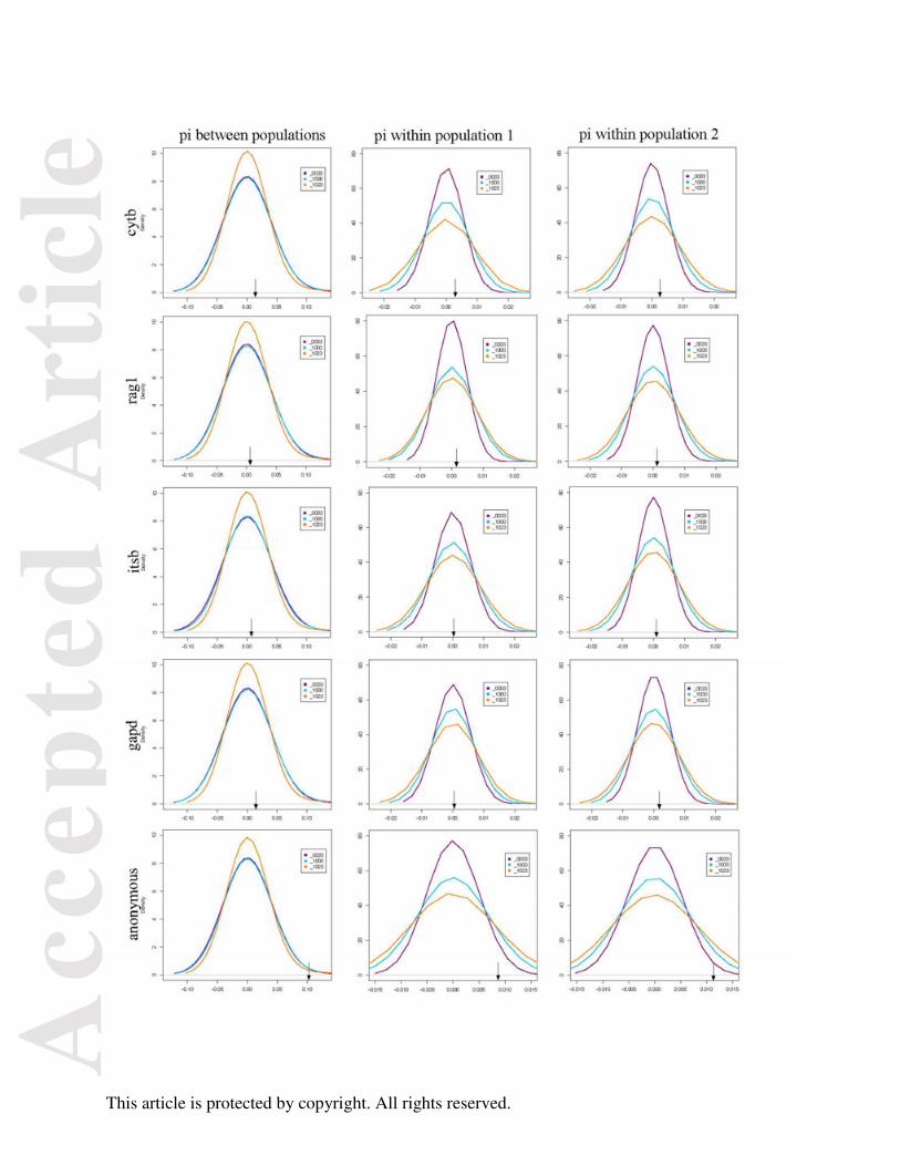
Density plots for each summary statistic from the ABC vector was plotted individually

for three models (0033, 1000, and 1023) using R 2.15.1 to assess model adequacy and any bias

in the summary statistics used for the ABC analysis (Fig. 6). Each summary statistic for the three

models share a similar distribution and the empirical estimates are well within this distribution. If

Acc

epte

d A

rtic

le


the summary statistics were biased we would expect the distribution for a given summary

statistic to be different under a different model. If the models could not somehow represent the

data, the empirical summary statistic would fall outside the PPS distribution. Furthermore, the

correlation between the number of parameters and the PP (R2 = 0.06, p = 0.002) and between the

number of parameters and the MED (R2 = 0.04, p = 0.01) is extremely weak; this bolsters the

argument of Beaumont et al. (2010) that the dimensionality of models does not influence the

calculation of the PP in phylogeographic model comparison.

Conclusions

Our ABC model selection procedure enabled us to identify a demographic model that is

both a good fit to the data (MED1023 = 0.956; final PP1023 > 0.99) and consistent with known

facts regarding the geologic history of the inland temperate rain forest. Plethodon idahoensis has

occupied this region for millions of years (Carstens et al. 2005), but recurrent glaciation during

the Pleistocene forced the species into two refugia located within the Clearwater River drainage.

Like many other temperate species (Hewitt 2004), available data indicate that the Pleistocene

climatic fluctuations had a substantial impact on the population genetic structure of P.

idahoensis. Our results imply strongly that these refugia were separated latitudinally (i.e., into

northern and southern refugia), and that this separation is responsible for the northern-southern

population genetic structure observed here. We also find support for population expansion,

particularly in the northern populations, and the results suggest that gene flow likely occurs over

the ridge separating the Lochsa and Selway rivers in central Idaho.

Researchers have been reluctant to adopt demographic model choice with ABC as a tool

for phylogeographic inference, and there are few examples of investigations that rely on this

Acc

epte

d A

rtic

le


approach. It is unlikely that this reluctance is due to a mistrust of ABC methods in general, or to

latent concerns about the applicability of the methods, as many researchers have utilized

msBayes, arguably a more complex and (due to the requirement of comparative data) less

applicable method developed by Hickerson et al. (2007). Rather, researchers in non-model

systems may find it difficult to parameterize models due to a lack of prior information, and thus

are hesitant to rely only on their intuition to develop a prior set of models to analyze. Model

choice with ABC offers a great deal of promise to phylogeographic investigations in non-model

systems, but only if the models in the comparison set can be identified in a systematic (and non-

biased) manner. We illustrate here that the posterior probabilities in these comparisons are

dependent on the composition of the model set, and develop an approach for identifying models

for inclusion in a model set that allows a wide range of models to be considered. We first

parameterized a large set of possible models, then conducted a preliminary comparison of all

models, before selecting only those models with a greater PP than expected by chance for

inclusion in the final comparison. PPS were used to check for model adequacy and bias in

summary statistics. While this approach may be criticized as being ad hoc, it is decidedly less so

than one that only considers models proposed by previous work or choses them based only on

the intuition of researchers; all models in such sets could be poor (as in our empirical example)

but one could nevertheless receive a high relative posterior probability. Our work demonstrates

that careful consideration of the composition of the model set is vital to ABC model-choice

experiments and that more attention should be devoted to this issue.

Acc

epte

d A

rtic

le


Acknowledgements

We appreciate comments and discussion from Jeremy Brown, Mike Hickerson, Naoki

Takebayashi, Melissa DeBiasse, Sarah Hird, John McVay, Noah Reid, and Jordan Satler. We

thank Matt Demarest, who helped with the scripting process. We value suggestions from

anonymous reviewers that improved previous versions of this manuscript, and appreciate the

patience shown by AE Stone while additional simulations were being conducted. Funding was

provided by NSF DEB-0918212 to BCC and the SSAR laboratory grant to TAP.

References

Beaumont MA (2010) Approximate Bayesian Computation in Evolution and Ecology. Annual

Reviews of Ecology, Evolution, and Systematics, 41, 379-406.

Beamont MA, Zhang WY, Balding DJ (2002) Approximate Bayesian computation in population

genetics. Genetics, 162, 2025-2035.

Beaumont MA, Nielsen R, Robert C, Hey J, Gaggioti O, Knowles LL, Estoup A, Panchal M,

Corander J, Hickerson MJ, Sisson SA, Fagundes N, Chikhi L, Beerli P, Vitalis R,

Cornuet JM, Huelsenbeck JP, Foll M, Yang Z, Rousset F, Balding DJ, Excoffier L (2010)

In defense of model-based inference in phylogeography. Molecular Ecology, 19, 436-

446.

Beerli P, Palczewski M (2010) Unified framework to evaluate panmixia and migration direction

among multiple sampling locations. Genetics, 185, 313-326.

Bertorelle G, Benazzo A, Mona S (2010) ABC as a flexible framework to estimate demography

over space and time: some cons, many pros. Molecular Ecology, 19, 2609-2625.

Acc

epte

d A

rtic

le


Box GEP, Draper NR (1987) Empirical Model-building and Response Surfaces. John Wiley &

Sons, Oxford, UK.

Carstens BC, Brennan RS, Chua V, Duffie CV, Harvey MG, Koch RA, McMahan CD, Nelson

BJ, Newman CE, Satler JD, Seeholzer G, Prosbic K, Tank DC, Sullivan J (2013) Model

selection as a tool for phylogeographic inference: An example from the willow Salix

melanopsis. Molecular Ecology, 22, 4014-4028.

Carstens BC, Brunsfeld SJ, Demboski JR, Good JM, Sullivan J (2005) Investigating the

evolutionary history of the Pacific Northwest mesic forest ecosystem: hypothesis testing

within and comparative phylogeographic framework. Evolution, 59, 1639-1652.

Carstens BC, Reid N, Stoute HN (2009) An information theoretical approach to phylogeography.

Molecular Ecology, 18, 4270-4282.

Carstens BC, Richards CL (2007) Integrating coalescent and ecological niche modeling in

comparative phylogeography. Evolution, 61, 1439-54.

Carstens BC, Stevenson AL, Degenhardt JD, Sullivan J (2004) Testing nested phylogenetic and

phylogeographic hypotheses in the Plethodon vandykei species group. Systematic

Biology, 53, 781-92.

Cornuet J, Ravigne V, Estoup A. 2010. Inference on population history and model checking

using DNA sequence and microsatellite data with the software DIYABC (v1.0). BMC

Bioinformatics, 11, 401.

Csillery K, Blum MGB, Gaggioti OE, Francois O (2011) Approximate Bayesian Computation

(ABC) in practice. Trends in Ecology & Evolution, 25, 410-418.

Drummond A, Ashton B, Buxton S, Cheung M, Cooper A, Duran C, Field M, Heled J, Kearse

M, Markowitz S (2011) Geneious v5. 4. Biomatters Ltd, Auckland, New Zealand.

Acc

epte

d A

rtic

le


Fagundes N, Ray DA, Beaumont MA, Neuenschwander S, Salzano FM, Bonatto SL, Excoffier L

(2007) Statisical evaluation of alternative models of human evolution. Proceedings of the

National Academy of Sciences of the USA, 104, 17614-17619.

Flot JF (2007) Champuru 1.0: a computer software for unraveling mixtures of two DNA

sequences of unequal lengths. Molecular Ecology Notes, 7, 974-977.

François O, Laval G. 2011. Deviance information criteria for model selection in approximate

Bayesian computation. Statistical Applications in Genetics and Molecular Biology, 10,

33.

Gelfand AE, Ghosh SK (1998). Model choice: A minimum posterior predictive loss approach.

Biometrika, 85, 1-11.

Hairston NG (1983) Growth, survival, and reproduction of Plethodon jordoni: trade-offs

between selective pressures. Copeia, 4, 1024-1035.

Hewitt G (2004) Genetic consequences of climatic oscillations in the Quaternary. Philosophical

Transactions of the Royal Society of London. Series B: Biological Sciences, 359, 183-

195.

Hey J, Nielsen R (2007) Integration within the Felsenstein equation or improved Markov chain

Monte Carlo methods in population genetics. Proceedings of the National Academy of

Sciences of the USA, 104, 2785-2790.

Hickerson MJ, Stahl E, Takebayashi N (2007) MSBayes: Pipeline for testing comparative

phylogeographic histories using hierarchical approximate Bayesian computation. BMC

Bioinformatics, 8, 268.

Hudson RR (2002) Generating samples under a Wright-Fisher neutral model of genetic variation.

Bioinformatics, 18, 337-338.

Acc

epte

d A

rtic

le


Kass RE, Raftery AE (1995). Bayes Factors. Journal of the American Statistical Association 90,

773-795.

Knowles LL (2009) Statistical Phylogeography. Annual Reviews of Ecology, Evolution, and

Systematics, 40, 593-612.

Koopman MM, Carstens BC (2010) Inferring population structure and demographic parameters

across a riverine barrier in the carnivorous plant Sarracenia alata (Sarraceniaceae).

Conservation Genetics, 11, 2027-2038.

Laval G, Patin E, Barreiro LB, Quintana-Murci L (2010) Formulating a historical and

demographic model of recent human evolution based on resequencing data from

noncoding regions. Plos One, 5, e10284.

Mahoney MJ (2004) Molecular systematics and phylogeography of the Plethodon elongatus

species group: combining phylogenetic and population genetic methods to investigate

species history. Molecular Ecology, 13, 149-166.

Marin JM, Pillai N, Robert C, Rousseau J (2011) Evaluating statistic appropriateness for

Bayesian model choice. HAL : hal-00641487, version 1.

Mead LS, Clayton DR, Nauman RS, Olson DH, Pfrender ME (2005) Newly discovered

populations of salamanders from Siskiyou County California represent a species distinct

from Plethodon stormi. Herpetologica, 61, 158-177.

Peter BM, Wegman D, Excoffier L (2010) Distinguishing between population bottleneck and

population subdivision by a Bayesian model choice procedure. Molecular Ecology, 19,

4648–4660.

Pond SLK, Frost SDW (2005) Datamonkey: rapid detection of selective pressure on individual

sites of codon alignments. Bioinformatics, 21, 2531-2533.

Acc

epte

d A

rtic

le


Pond SLK, Posada D, Gravenor MB, Woelk CH, Frost SDW (2006) GARD: a genetic algorithm

for recombination detection. Bioinformatics, 22, 3096-3098.

Pritchard JK, Seielstad MT, Perez-Lezaun A, Feldman MW (1999) Population Growth of

Human Y Chromosomes: A Study of Y Chromosome Microsatellites. Molecular Biology

and Evolution, 16, 1791-1798.

Provan J, Maggs CA (2012) Unique genetic variation at a species's rear edge is under threat from

global climate change. Proceedings of the Royal Society of London B 279, 39-47.

R Core Team (2012) R: A language and environment for statistical computing. R Foundation for

Statistical Computing Vienna Austria.

Ratmann O, Andrieu C, Wiuf C, Richardson S (2009) Model criticism based on likelihood-free

inference, with an application to protein network evolution. Proceedings of the National

Academy of Sciences USA, 106, 10576-10581.

Robert CP, Cornuet JM, Marin JM, Pillai NS (2011) Lack of confidence in approximate

Bayesian computation model choice. Proceedings of the National Academy of Sciences

USA, 108, 15112-15117.

Rozas J, Sánchez-Delbarrio JC, Messeguer X, Rozas R (2003) DnaSP, DNA polymorphism

analyses by the coalescent and other methods. Bioinformatics, 19, 2496-2497.

Salter JD, Carstens BC, Hedin M (2013) Multilocus species delimitation in a complex of

morphologically conserved trapdoor spiders (Mygalomorphae, Antrodiaetidae,

Aliatypus). Systematic Biology 62, 805-823.

Smith CI, Tank S, Godsoe W, Levenick J, Strand E, Esque T, Pellmyr O (2011) Comparative

phylogeography of a coevolved community: Concerted population genetic expansions in

Joshua Trees and four Yucca moths. PLoS One, 6, e25628.

Acc

epte

d A

rtic

le


Smith M, Green D (2005) Dispersal and the metapopulation paradigm in amphibian ecology and

conservation: are all amphibian populations metapopulations? Ecography, 28, 110-128.

Smith G, Lohse K, Etges WJ, Ritchie MG (2012) Model-based comparisons of phylogeographic

scenarios resolve the intraspecific divergence of cactophilic Drosophila mojavensis.


Sousa VC, Fritz M, Beaumont MA, Chikhi L (2009) Approximate Bayesian computation

without summary statistics: The case of admixture. Genetics, 181, 1507-1519.

Stephens M, Smith NJ, Donnelly P (2001) A new statistical method for haplotype reconstruction

from population data. Genetics, 68, 978-989.

Templeton AR (2009) Statistical hypothesis testing in intraspecific phylogeography: nested clade

phylogeographical analysis vs. approximate Bayesian computation. Molecular Ecology,

18, 319-331.

Templeton AR (2010) Coalescent-based, maximum likelihood inference in phylogeography.


Tsai Y-H, Carstens BC (2013) Assssing model fit in phylogeographic investigations: An

example from the North American willow Salix melanopsis. Journal of Biogeography,

40, 131-141.

Wilson Jr. AG, Larsen Jr. JH (1998) Biogeographic analysis of the Coeur d'Alene salamander

(Plethodon idahoensis). Northwest Science, 72, 111-115.

Acc

epte

d A

rtic

le


Author contributions TAP conducted the molecular labwork, participated in design of the study, performed statistical

analysis, wrote the scripts used in data simulation, and drafted the manuscript. BCC collected the

samples, participated in the design of the study, contributed to script development, supervised the

research, and drafted the manuscript. Both authors read and approved the final manuscript.

Data Accessibility

Sequences for all genes have been deposited in GenBank under the following accession numbers

JX978543-JX978577 and in DRYAD doi:10.5061/dryad.8kq65. Model prior and scripts can also

be found at doi:10.5061/dryad.8kq65.

Figure Legends

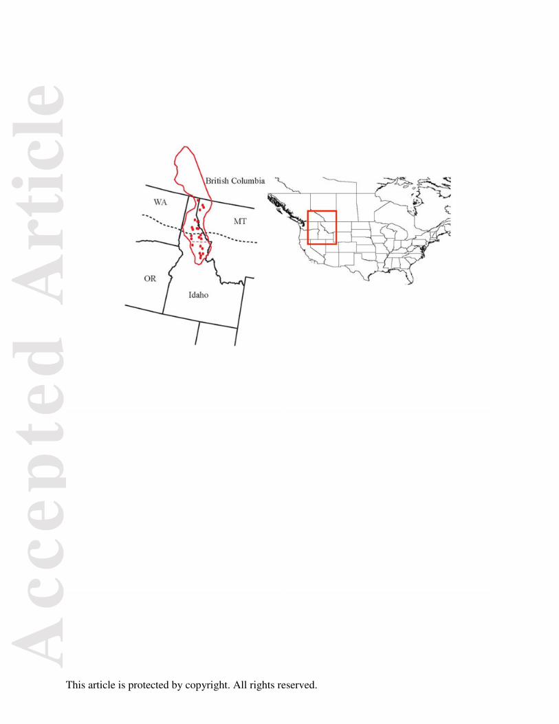
Fig. 1. Sampling localities of Plethodon idahoensis in the Pacific Northwest, US.

Dark line is its distribution in Idaho, Montana, and British Columbia. The dotted line within the

distribution delineates the northern (population 2) and southern (population 1) river drainages.

The large dotted line represents the extent of the ice sheets during the last glacial maximum.

Fig. 2. Numeric coding for demographic models being tested. All models are identified with

a 4-digit number that describes the parameter combination associated with a particular model

corresponding to population divergence, θ = 4Nem, migration rates, and the extrinsic rate of

population expansion. Each parameter can be assigned to the northern (subscript 1) or southern

(subscript 2) populations in one of several combinations. Uniform priors are based on previous

Plethodon work and occupy the full range of biologically reasonable values and are according to

ms (Hudson 2002) documentation.

Acc

epte

d A

rtic

le


Fig. 3. Diagram of the five demographic models (Carstens et al. 2009; Carstens & Richards

2007; Carstens et al. 2004) used for the first round 5-model ABC analysis. Each model includes

one or more parameters, is labeled by a numeric code, and includes its posterior probability in

the initial ABC model choice analysis.

Fig. 4. Simulation testing to investigate the performance of ABC model choice as a function of

the number of models. The prior probability (blue line), averaged probability of the most-

represented model in a selection equal to the size of the posterior (red line), posterior probability

of the true model (orange line) and the median Bayes factor (dotted line) are shown.

Fig. 5. Results from 143-model ABC analysis. Black bars are relative posterior probabilities.

Dotted line is the prior probability. Solid line is the average highest PP observed by random

chance. Only the 5-model test models and models with the highest and lowest PP are labeled for

clarity. All model PP and MED values are in Table 3.

Fig. 6. Density plots for each summary statistic in the vector used for all analyses for the

following models. Model 0033: island with no change in θ, migration in both directions and

expansion in both populations. Model 1000: isolation model with no change in θ, no migration,

and no expansion. Model 1023: isolation model with no change in θ, migration from population

2 to 1, and expansion in both populations. Black arrows indicate where the empirical estimate

falls.

Acc

epte

d A

rtic

le


Table 1. Summary statistics for 5 loci. Shown for each locus are the source of the primers, the

length (bp) and six summary statistics: nucleotide diversity (π), the number of segregating sites

(SS), Tajima's D (D), nucleotide diversity within the northern (πW1) and southern (πW2)

populations, and nucleotide diversity between the northern and southern populations (πB).

Locus Source π segregating sites (SS)

Tajima's D (D)

π within pop1 (πW1)

π within pop2 (πW2)

π between pops (πB)

cytb Carstens et al. 2004 0.0082 27 -0.9358 0.0047 0.0050 0.0113

RAG1 Weins et al. 2006 0.0024 13 -0.1791 0.0017 0.0020 0.0021

ITS1 Hillis and Dixon 1991 0.0019 4 -0.1810 0.0000 0.0023 0.0021

Gapd Dolman and Phillips

2004 0.0032 8 -0.1153 0.0002 0.0036 0.0043

anonymous this study 0.0146 21 2.2552 0.0095 0.0160 0.0157

Table 2. Population parameter estimates. Estimates are from mean values in posterior

distributions. 95% CI are shown in parentheses below the estimates. Models that lack a given

parameter are marked with an 'na'.

Model θ θ1 θ2 τ m1 m2 γ1 γ2

1000

0.079 (0.059-0.097) na na

1.569 (1.176-1.961) na na na na

1023

0.089 (0.061-0.117) na na

1.933 (1.507-2.359) na

2.858 (2.349-3.368)

3.776 (-0.668-8.220)

1.678 (0.720-2.635)

Acc

epte

d A

rtic

le


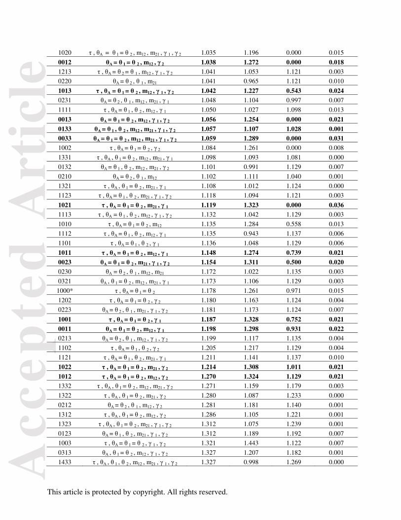
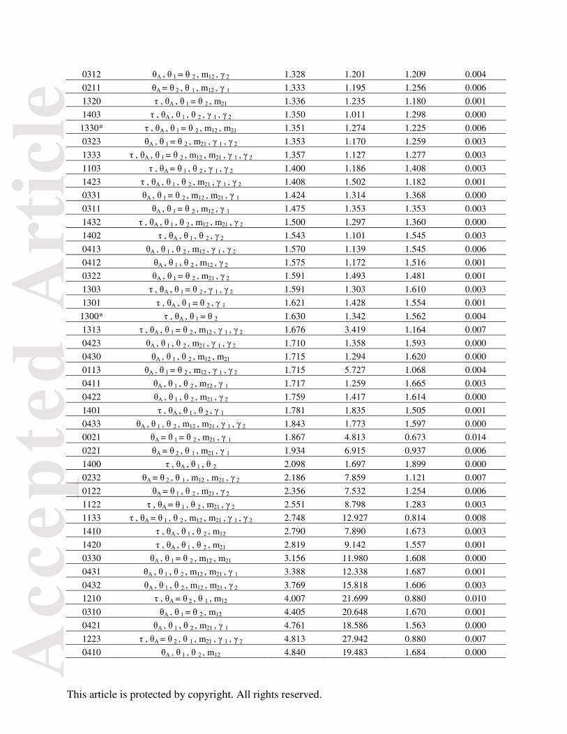
Table 3. List of all 143 models included in analyses. Model = τθmγ

Model numbering scheme is followed by the parameters included in that model (see Fig. 2).

They are ranked from lowest to highest MED including the StDev and median. The initial five-

model ABC test models are indicated by an asterisk ‘*’. The 22 models with PP above the

random expectation from the 143-model test are bolded.

Model Parameters Mean StDev Median Posterior

Probability

1030 τ , θΑ = θ 1= θ 2 , m12 , m21 0.792 1.124 0.000 0.024 1232 τ , θΑ = θ 2 , θ 1 , m12 , m21 , γ 2 0.822 0.856 0.772 0.007

1200 τ , θΑ = θ 2 , θ 1 0.836 0.985 0.499 0.004

1222 τ , θΑ = θ 2 , θ 1 , m21 , γ 2 0.846 0.982 0.542 0.006

1220 τ , θΑ = θ 2 , θ 1 , m21 0.849 0.957 0.647 0.006

1231 τ , θΑ = θ 2 , θ 1 , m12 , m21 , γ 1 0.863 0.877 0.859 0.006

1221 τ , θΑ = θ 2 , θ 1 , m21 , γ 1 0.870 0.878 0.862 0.011

1031 τ , θΑ = θ 1 = θ 2 , m12 , m21 , γ 1 0.886 1.133 0.000 0.020 1230 τ , θΑ = θ 2 , θ 1 , m12 , m21 0.917 0.937 0.880 0.006

1033 τ , θΑ = θ 1 = θ 2 , m12 , m21 , γ 1 , γ 2 0.923 1.170 0.000 0.018 0131 θΑ = θ 1 , θ 2 , m12 , m21 , γ 1 0.930 1.024 0.779 0.007

0130 θΑ = θ 1 , θ 2 , m12 , m21 0.949 0.881 1.055 0.010

1023 τ , θΑ = θ 1 = θ 2 , m21 , γ 1 , γ 2 0.956 1.154 0.000 0.024 1201 τ , θΑ = θ 2 , θ 1 , γ 1 0.975 1.026 0.866 0.006

0030 θΑ = θ 1 = θ 2 , m12 , m21 0.977 1.210 0.000 0.024 1211 τ , θΑ = θ 2 , θ 1 , m12 , γ 1 0.990 1.042 0.927 0.007

0020 θΑ = θ 1 = θ 2 , m12 , m21 0.991 1.264 0.000 0.017 1132 τ , θΑ = θ 1 , θ 2 , m12 , m21 , γ 2 0.995 0.981 0.986 0.007

0031 θΑ = θ 1 = θ 2 , m12 , m21 , γ 1 0.996 1.303 0.000 0.020

0022 θΑ = θ 1 = θ 2 , m21 , γ 2 1.003 1.241 0.000 0.025 1131 τ , θΑ = θ 1 , θ 2 , m12 , m21 , γ 1 1.011 0.967 1.013 0.004

1032 τ , θΑ = θ 1 = θ 2 , m12 , m21 , γ 2 1.013 1.212 0.000 0.031 1212 τ , θΑ = θ2 , θ 1 , m12 , γ 2 1.015 0.986 1.083 0.003

1233 τ , θΑ = θ 2 , θ 1 , m12 , m21 , γ 1 , γ 2 1.021 0.946 1.121 0.010

1203 τ , θΑ = θ 2 , θ 1 , γ 1 , γ 2 1.024 1.058 1.002 0.010

0233 θΑ = θ 2 , θ 1 , m12 , m21 , γ 1 , γ 2 1.026 0.985 1.118 0.004

1110 τ , θΑ = θ 1 , θ 2 , m12 , γ 1 1.030 1.003 1.118 0.007

0222 θΑ = θ 2 , θ 1 , m21 , γ 2 1.031 1.112 0.921 0.008

1130 τ , θΑ = θ 1 , θ 2 , m12 , m21 1.031 0.976 1.084 0.006

0112 θΑ = θ 1 , θ 2 , m12 , γ 2 1.032 0.991 1.121 0.007

0032 θΑ = θ 1 = θ 2 , m12 , m21 , γ 2 1.033 1.212 0.000 0.020 0110 θΑ = θ 1 , θ 2 , m12 , γ 1 1.034 1.031 1.070 0.004

Acc

epte

d A

rtic

le


1020 τ , θΑ = θ 1 = θ 2 , m12 , m21 , γ 1 , γ 2 1.035 1.196 0.000 0.015

0012 θΑ = θ 1 = θ 2 , m12 , γ 2 1.038 1.272 0.000 0.018 1213 τ , θΑ = θ 2 = θ 1 , m12 , γ 1 , γ 2 1.041 1.053 1.121 0.003

0220 θΑ = θ 2 , θ 1 , m21 1.041 0.965 1.121 0.010

1013 τ , θΑ = θ 1 = θ 2 , m12 , γ 1 , γ 2 1.042 1.227 0.543 0.024 0231 θΑ = θ 2 , θ 1 , m12 , m21 , γ 1 1.048 1.104 0.997 0.007

1111 τ , θΑ = θ 1 , θ 2 , m12 , γ 1 1.050 1.027 1.098 0.013

0013 θΑ = θ 1 = θ 2 , m12 , γ 1 , γ 2 1.056 1.254 0.000 0.021

0133 θΑ = θ 1 , θ 2 , m12 , m21 , γ 1 , γ 2 1.057 1.107 1.028 0.001

0033 θΑ = θ 1 = θ 2 , m12 , m21 , γ 1 , γ 2 1.059 1.289 0.000 0.031 1002 τ , θΑ = θ 1 = θ 2 , γ 2 1.084 1.261 0.000 0.008

1331 τ , θΑ , θ 1 = θ 2 , m12 , m21 , γ 1 1.098 1.093 1.081 0.000

0132 θΑ = θ 1 , θ 2 , m12 , m21 , γ 2 1.101 0.991 1.129 0.007

0210 θΑ = θ 2 , θ 1 , m12 1.102 1.111 1.040 0.001

1321 τ , θΑ , θ 1 = θ 2 , m21 , γ 1 1.108 1.012 1.124 0.000

1123 τ , θΑ = θ 1 , θ 2 , m21 , γ 1 , γ 2 1.118 1.094 1.121 0.003

1021 τ , θΑ = θ 1 = θ 2 , m21 , γ 1 1.119 1.323 0.000 0.036 1113 τ , θΑ = θ 1 , θ 2 , m12 , γ 1 , γ 2 1.132 1.042 1.129 0.003

1010 τ , θΑ = θ 1 = θ 2 , m12 1.135 1.284 0.558 0.013

1112 τ , θΑ = θ 1 , θ 2 , m12 , γ 1 1.135 0.943 1.137 0.006

1101 τ , θΑ = θ 1 , θ 2 , γ 1 1.136 1.048 1.129 0.006

1011 τ , θΑ = θ 1 = θ 2 , m12 , γ 1 1.148 1.274 0.739 0.021

0023 θΑ = θ 1 = θ 2 , m21 , γ 1 , γ 2 1.154 1.311 0.500 0.020 0230 θΑ = θ 2 , θ 1 , m12 , m21 1.172 1.022 1.135 0.003

0321 θΑ , θ 1 = θ 2 , m12 , m21 , γ 1 1.173 1.106 1.129 0.003

1000* τ , θΑ = θ 1 = θ 2 1.178 1.261 0.971 0.015

1202 τ , θΑ = θ 1 = θ 2 , γ 2 1.180 1.163 1.124 0.004

0223 θΑ = θ 2 , θ 1 , m21 , γ 1 , γ 2 1.181 1.173 1.124 0.007

1001 τ , θΑ = θ 1 = θ 2 , γ 1 1.187 1.328 0.752 0.021

0011 θΑ = θ 1 = θ 2 , m12 , γ 1 1.198 1.298 0.931 0.022 0213 θΑ = θ 2 , θ 1 , m12 , γ 1 , γ 2 1.199 1.117 1.135 0.004

1102 τ , θΑ = θ 1 , θ 2 , γ 2 1.205 1.217 1.129 0.004

1121 τ , θΑ = θ 1 , θ 2 , m21 , γ 1 1.211 1.141 1.137 0.010

1022 τ , θΑ = θ 1 = θ 2 , m21 , γ 2 1.214 1.308 1.011 0.021

1012 τ , θΑ = θ 1 = θ 2 , m12 , γ 2 1.270 1.324 1.129 0.021 1332 τ , θΑ , θ 1 = θ 2 , m12 , m21 , γ 2 1.271 1.159 1.179 0.003

1322 τ , θΑ , θ 1 = θ 2 , m21 , γ 2 1.280 1.087 1.233 0.000

0212 θΑ = θ 2 , θ 1 , m12 , γ 2 1.281 1.181 1.140 0.001

1312 τ , θΑ , θ 1 = θ 2 , m12 , γ 2 1.286 1.105 1.221 0.001

1323 τ , θΑ , θ 1 = θ 2 , m21 , γ 1 , γ 2 1.312 1.075 1.239 0.001

0123 θΑ = θ 1 , θ 2 , m21 , γ 1 , γ 2 1.312 1.189 1.192 0.007

1003 τ , θΑ = θ 1 = θ 2 , γ 1 , γ 2 1.321 1.443 1.122 0.007

0313 θΑ , θ 1 = θ 2 , m12 , γ 1 , γ 2 1.327 1.207 1.182 0.001

1433 τ , θΑ , θ 1 , θ 2 , m12 , m21 , γ 1 , γ 2 1.327 0.998 1.269 0.000

Acc

epte

d A

rtic

le


0312 θΑ , θ 1 = θ 2 , m12 , γ 2 1.328 1.201 1.209 0.004

0211 θΑ = θ 2 , θ 1 , m12 , γ 1 1.333 1.195 1.256 0.006

1320 τ , θΑ , θ 1 = θ 2 , m21 1.336 1.235 1.180 0.001

1403 τ , θΑ , θ 1 , θ 2 , γ 1 , γ 2 1.350 1.011 1.298 0.000

1330* τ , θΑ , θ 1 = θ 2 , m12 , m21 1.351 1.274 1.225 0.006

0323 θΑ , θ 1 = θ 2 , m21 , γ 1 , γ 2 1.353 1.170 1.259 0.003

1333 τ , θΑ , θ 1 = θ 2 , m12 , m21 , γ 1 , γ 2 1.357 1.127 1.277 0.003

1103 τ , θΑ = θ 1 , θ 2 , γ 1 , γ 2 1.400 1.186 1.408 0.003

1423 τ , θΑ , θ 1 , θ 2 , m21 , γ 1 , γ 2 1.408 1.502 1.182 0.001

0331 θΑ , θ 1 = θ 2 , m12 , m21 , γ 1 1.424 1.314 1.368 0.000

0311 θΑ , θ 1 = θ 2 , m12 , γ 1 1.475 1.353 1.353 0.003

1432 τ , θΑ , θ 1 , θ 2 , m12 , m21 , γ 2 1.500 1.297 1.360 0.000

1402 τ , θΑ , θ 1 , θ 2 , γ 2 1.543 1.101 1.545 0.003

0413 θΑ , θ 1 , θ 2 , m12 , γ 1 , γ 2 1.570 1.139 1.545 0.006

0412 θΑ , θ 1 , θ 2 , m12 , γ 2 1.575 1.172 1.516 0.001

0322 θΑ , θ 1 = θ 2 , m21 , γ 2 1.591 1.493 1.481 0.001

1303 τ , θΑ , θ 1 = θ 2 , γ 1 , γ 2 1.591 1.303 1.610 0.003

1301 τ , θΑ , θ 1 = θ 2 , γ 1 1.621 1.428 1.554 0.001

1300* τ , θΑ , θ 1 = θ 2 1.630 1.342 1.562 0.004

1313 τ , θΑ , θ 1 = θ 2 , m12 , γ 1 , γ 2 1.676 3.419 1.164 0.007

0423 θΑ , θ 1 , θ 2 , m21 , γ 1 , γ 2 1.710 1.358 1.593 0.000

0430 θΑ , θ 1 , θ 2 , m12 , m21 1.715 1.294 1.620 0.000

0113 θΑ , θ 1 = θ 2 , m12 , γ 1 , γ 2 1.715 5.727 1.068 0.004

0411 θΑ , θ 1 , θ 2 , m12 , γ 1 1.717 1.259 1.665 0.003

0422 θΑ , θ 1 , θ 2 , m21 , γ 2 1.759 1.417 1.614 0.000

1401 τ , θΑ , θ 1 , θ 2 , γ 1 1.781 1.835 1.505 0.001

0433 θΑ , θ 1 , θ 2 , m12 , m21 , γ 1 , γ 2 1.843 1.773 1.597 0.000

0021 θΑ = θ 1 = θ 2 , m21 , γ 1 1.867 4.813 0.673 0.014

0221 θΑ = θ 2 , θ 1 , m21 , γ 1 1.934 6.915 0.937 0.006

1400 τ , θΑ , θ 1 , θ 2 2.098 1.697 1.899 0.000

0232 θΑ = θ 2 , θ 1 , m12 , m21 , γ 2 2.186 7.859 1.121 0.007

0122 θΑ = θ 1 , θ 2 , m21 , γ 2 2.356 7.532 1.254 0.006

1122 τ , θΑ = θ 1 , θ 2 , m21 , γ 2 2.551 8.798 1.283 0.003

1133 τ , θΑ = θ 1 , θ 2 , m12 , m21 , γ 1 , γ 2 2.748 12.927 0.814 0.008

1410 τ , θΑ , θ 1 , θ 2 , m12 2.790 7.890 1.673 0.003

1420 τ , θΑ , θ 1 , θ 2 , m21 2.819 9.142 1.557 0.001

0330 θΑ , θ 1 = θ 2 , m12 , m21 3.156 11.980 1.608 0.000

0431 θΑ , θ 1 , θ 2 , m12 , m21 , γ 1 3.388 12.338 1.687 0.001

0432 θΑ , θ 1 , θ 2 , m12 , m21 , γ 2 3.769 15.818 1.606 0.003

1210 τ , θΑ = θ 2 , θ 1 , m12 4.007 21.699 0.880 0.010

0310 θΑ , θ 1 = θ 2 , m12 4.405 20.648 1.670 0.001

0421 θΑ , θ 1 , θ 2 , m21 , γ 1 4.761 18.586 1.563 0.000

1223 τ , θΑ = θ 2 , θ 1 , m21 , γ 1 , γ 2 4.813 27.942 0.880 0.007

0410 θΑ , θ 1 , θ 2 , m12 4.840 19.483 1.684 0.000

Acc

epte

d A

rtic

le


0333 θΑ , θ 1 = θ 2 , m12 , m21 , γ 1 , γ 2 4.841 24.764 1.304 0.004

1411 τ , θΑ , θ 1 , θ 2 , m12 , γ 1 4.949 22.725 1.182 0.000

0320 θΑ , θ 1 = θ 2 , m21 5.184 25.275 1.771 0.000

1431 τ , θΑ , θ 1 , θ 2 , m12 , m21 , γ 1 5.539 28.987 1.440 0.000

1421 τ , θΑ , θ 1 , θ 2 , m21 , γ 1 5.618 22.805 1.418 0.001

1311 τ , θΑ , θ 1 = θ 2 , m12 , γ 1 5.721 32.177 1.137 0.001

0111 θΑ = θ 1 , θ 2 , m12 , γ 1 5.804 32.950 1.143 0.008

0420 θΑ , θ 1 , θ 2 , m21 6.037 28.946 1.629 0.001

1412 τ , θΑ , θ 1 , θ 2 , m12 , γ 2 6.186 23.177 1.611 0.003

0010 θΑ = θ 1 = θ 2 , m12 6.223 36.293 0.000 0.017

1413 τ , θΑ , θ 1 , θ 2 , m12 , γ 1 , γ 2 8.209 48.083 1.344 0.000

1430 τ , θΑ , θ 1 , θ 2 , m12 , m21 8.661 50.499 1.516 0.001

1422 τ , θΑ , θ 1 , θ 2 , m21 , γ 2 9.269 45.089 1.344 0.006

0121 θΑ = θ 1 , θ 2 , m21 , γ 1 9.369 56.607 1.327 0.004

1302 τ , θΑ , θ 1 = θ 2 , γ 2 9.386 44.243 1.233 0.004

0120 θΑ = θ 1 , θ 2 , m21 9.466 57.924 1.189 0.004

1310 τ , θΑ , θ 1 = θ 2 , m12 9.812 60.333 1.206 0.000

1100 τ , θΑ = θ 1 , θ 2 10.795 68.438 1.121 0.007

0332 θΑ , θ 1 = θ 2 , m12 , m21 , γ 2 13.053 82.999 1.415 0.004

1120 τ , θΑ = θ 1 , θ 2 , m21 14.667 54.818 1.365 0.007

X0X1* θΑ , γ 1 16.013 5.576 15.576 0.000

X0X0* θΑ 17.048 7.013 16.115 0.000

0000 θΑ = θ 1 = θ 2 116.825 42.505 116.338 0.000

Table 4. Results of the nested model comparison are shown, as well as the final comparison.

Model PP BF

Divergence models 1001 1011 1012

0.07 2.6 0.04 4.5 0.05 3.6

1013 0.05 3.6 1021 1022

0.11 1.6 0.11 1.6

1023 1030

0.18 1 0.07 2.6

1031 0.07 2.6 1032 1033

0.09 2.0 0.14 1.3

Island models 0010 0.08 2.3

Acc

epte

d A

rtic

le


0011 0012 0013 0020 0022 0023

0.08 2.3 0.12 1.5 0.04 4.5 0.10 1.8 0.12 1.5 0.06 3.0

0030 0031 0032

0.08 2.3 0.08 2.3 0.04 4.5

0033 0.18 1 Final comparison 1023 >0.9 0033 0

List of Supplemental Files

Supporting Information 1. Primer and PCR conditions

Supporting Information 2. Summary statistic testing

Supporting Information 3. ABC regression and threshold testing

Supporting Information 4. Replicate 5-model ABC results; R package ABC cross-validation with

subset of models

Supporting Information 5. Power analysis and regression information

Supporting Information 6. PP and MED on partitioned groups of models

Acc

epte

d A

rtic

le


model choice for phylogeographic inference using a large set of models

Documents