DEGREE PROJECT, IN , SECOND LEVELAUTOMATIC CONTROL

STOCKHOLM, SWEDEN 2015

Model Complexity and Coupling ofLongitudinal and Lateral Control inAutonomous Vehicles Using ModelPredictive Control

CHRISTIAN OLSSON

KTH ROYAL INSTITUTE OF TECHNOLOGY

SCHOOL OF ELECTRICAL ENGINEERING

ACKNOWLEDGEMENTS

A big thanks to my supervisor Jonas Mårtensson who introduced the thesis topic tome and gave invaluable feedback during our meetings. The biggest thanks to myco-supervisor Pedro Lima for assisting me throughout the whole thesis and givingfeedback on my work.

1

ABSTRACT

Autonomous vehicles and research pertaining to them have been an important topicin academia and industry in recent years. Developing controllers that enable vehi-cles to perform path and trajectory following is a diverse topic where many differentcontrol strategies are available. In this thesis, we focus on lateral and longitudinalcontrol of autonomous vehicles and two different control strategies are considered:a standard decoupled control and a new suggested coupled control.

In the decoupled control, the lateral controller consists of a linear time-varying modelpredictive controller (LTV-MPC) together with a PI-controller for the longitudinalcontrol. The coupled controller is a more complex LTV-MPC which handles bothlateral and longitudinal control. The objective is to develop both control strategiesand evaluate their design and performance through path following simulations in aMATLAB environment.

When designing the LTV-MPC, two vehicle models are considered: a kinematic modelwithout tyre dynamics and a dynamic bicycle model with tyre forces derived froma linear Pacejka model. A research on how model complexity affects tracking per-formance and solver times is also performed. In the end, the thesis presents thefindings of the different control strategies and evaluate them in terms of trackingperformance, solver time, and ease of implementation.

2

CONTENTS

1 Introduction 5

2 Background 7

3 Problem Formulation 12

4 Vehicle Modelling 134.1 Kinematic Vehicle Model . . . . . . . . . . . . . . . . . . . . . . . . . . . 134.2 Dynamical Vehicle Model . . . . . . . . . . . . . . . . . . . . . . . . . . . 14

5 Vehicle Control 185.1 System Overview . . . . . . . . . . . . . . . . . . . . . . . . . . . . . . . . 185.2 Lateral Control . . . . . . . . . . . . . . . . . . . . . . . . . . . . . . . . . 185.3 Longitudinal Control . . . . . . . . . . . . . . . . . . . . . . . . . . . . . . 195.4 Decoupled Control . . . . . . . . . . . . . . . . . . . . . . . . . . . . . . . 195.5 Coupled Control . . . . . . . . . . . . . . . . . . . . . . . . . . . . . . . . 205.6 Model Predictive Control . . . . . . . . . . . . . . . . . . . . . . . . . . . 21

5.6.1 Introduction to MPC . . . . . . . . . . . . . . . . . . . . . . . . . . 215.6.2 MPC for tracking . . . . . . . . . . . . . . . . . . . . . . . . . . . . 225.6.3 MPC for Path Following . . . . . . . . . . . . . . . . . . . . . . . . 235.6.4 Linear MPC . . . . . . . . . . . . . . . . . . . . . . . . . . . . . . . 255.6.5 Turn MPC into Quadratic Programming . . . . . . . . . . . . . . 265.6.6 Tuning . . . . . . . . . . . . . . . . . . . . . . . . . . . . . . . . . . 285.6.7 Coupled Path Following MPC . . . . . . . . . . . . . . . . . . . . . 30

5.7 Speed Profiling . . . . . . . . . . . . . . . . . . . . . . . . . . . . . . . . . 30

6 Simulation Setup 346.1 System Overview . . . . . . . . . . . . . . . . . . . . . . . . . . . . . . . . 346.2 Waypointing - Creating the References . . . . . . . . . . . . . . . . . . . 356.3 Simulation Path . . . . . . . . . . . . . . . . . . . . . . . . . . . . . . . . . 366.4 Performance Measurement and Tuning . . . . . . . . . . . . . . . . . . . 366.5 MPC Solver Evaluation . . . . . . . . . . . . . . . . . . . . . . . . . . . . . 386.6 Tuning the Controllers . . . . . . . . . . . . . . . . . . . . . . . . . . . . . 39

3

7 Simulation Results 407.1 Decoupled Control . . . . . . . . . . . . . . . . . . . . . . . . . . . . . . . 40

7.1.1 Kinematic Decoupled MPC on Kinematic Model . . . . . . . . . 407.1.2 Kinematic Decoupled MPC on Dynamic Model . . . . . . . . . . 427.1.3 Dynamic Lateral MPC on Dynamic Model . . . . . . . . . . . . . 427.1.4 Dynamic Decoupled MPC on Dynamic Model . . . . . . . . . . . 43

7.2 Coupled Control . . . . . . . . . . . . . . . . . . . . . . . . . . . . . . . . 447.2.1 Kinematic Coupled MPC on Dynamic Model . . . . . . . . . . . 447.2.2 Dynamic Coupled MPC on Dynamic Model . . . . . . . . . . . . 44

7.3 Lateral Stability Test . . . . . . . . . . . . . . . . . . . . . . . . . . . . . . 457.4 Speed Profile Evaluation . . . . . . . . . . . . . . . . . . . . . . . . . . . . 46

8 Discussion 488.1 Model Complexity in MPC . . . . . . . . . . . . . . . . . . . . . . . . . . . 488.2 Longitudinal Control . . . . . . . . . . . . . . . . . . . . . . . . . . . . . . 488.3 Coupled vs. Decoupled Lateral and Longitudinal Control . . . . . . . . 498.4 Use of a More Conservative Speed Profile . . . . . . . . . . . . . . . . . . 508.5 Tuning Strategies . . . . . . . . . . . . . . . . . . . . . . . . . . . . . . . . 518.6 Comments on the Complete System . . . . . . . . . . . . . . . . . . . . . 51

9 Conclusion 53

10 Future Work 55

4

CHAPTER 1

INTRODUCTION

The cruise control in vehicles is far older than people believe, dating back to early1900’s and was an adaptation from James Watt and Matthew Boulton’s steam en-gine control. The modern version of a cruise control was invented 1948 by the me-chanical engineer Ralph Teetor and it was capable of keeping the speed of a vehicleconstant on any road [1]. The cruise controller can be seen as the first step towardsautonomous, or self driving, cars. The cruise controller is an example of a longitu-dinal controller, affecting the acceleration and deceleration of a car. The next stepin autonomous vehicle control would be lateral control, which is how to make thevehicle steer itself.

In 2005, a group of engineers at Google won the 2005 DARPA Grand Challenge fortheir work on Google’s self driving car [2]. Using a wide range of sensors, the carhad both longitudinal and lateral control and could successfully navigate on pub-lic roads in the USA. This autonomous Toyota Prius caught the public’s attentionand after 2005 the world has seen a rise in autonomous vehicle technology. Morerecently, German car manufacturer Audi has produced a autonomous R7 race carwhich has shown incredibly performance on race tracks, producing lap times on thesame level as professional racing drivers [3]. When autonomous vehicles were firstintroduced, it was a mere proof of concept that worked on closed roads and highlysupervised by engineers, but today there are several car manufacturers who wishto introduce autonomous vehicle systems to the public, including Mercedes, Volvoand Scania.

Scania leads a project called iQmatic which aims to introduce autonomous trucksand heavy duty vehicles in closed environments, such as mines. In this vast projectlies topics of vehicle control, path finding, obstacle avoidance, and many more whichall together will soon produce a fully autonomous Scania truck. A part of this projectinvolves the use of model predictive controllers (MPC) for lateral control of the truck.The benefit of using MPC is that it is a very fast optimization based control that hasproved to be suitable for task such as path and trajectory following. The use of MPCin autonomous vehicles is a blooming research field and many aspects of control,

5

stability, implementation, among others, are being researched every day.

A specific research topic pertains to vehicle modelling and control. The majority ofmathematical vehicle models are coupled, meaning that trying to change one stateof the vehicle is likely going to affect another state. A common control strategy is tohave separate control for lateral and longitudinal dynamics, where the most com-mon being a stand-alone lateral controller together with an ordinary cruise con-troller. This way, an engineer can control what speed the vehicle will travel and letthe lateral controller handle the steering. A more advanced version of this is usingone lateral controller and one longitudinal controller that can control speed, ac-celeration and deceleration of the vehicle. These two controllers, when they workindependently are called decoupled control and it is a common control strategy forautonomous vehicles.

In this thesis, we investigate if the fact that the vehicle models are coupled can beused to create a coupled control strategy. The idea being that a combination of lateraland longitudinal control can work together and be beneficial for the autonomoussystem. We will also research how model complexity in MPC affects performanceand if it is possible to perform path following with lower model complexity in theMPC than in the controlled vehicle.

6

CHAPTER 2

BACKGROUND

The road to a completely autonomous vehicle crosses a vast amount of engineeringfields that all need to be integrated into one complete system. In the article on Mer-cedes’ autonomous car "Bertha", the authors give a detailed view of what parts areneeded to complete the system [4]. An overview of the system is shown in Figure2.0.1 and the Bertha system has here been simplified into four layers. The top layercontains hardware and sensors. Bertha has a great amount of camera and radarsensors that gives the vehicle a situational awareness and helps the car interact withits environment. On the inside, there are vehicle sensors which measures and ob-serves the internal states of the car, including engine, steering and throttle control.The second layer contains all tools for performing localization and intepreting thesensor data, or perception. A high resolution GPS keeps track of the global positionof the car that together with a detailed digital map tells the driving system where itis and what restrictions the current position imposes on the vehicle. Examples ofinformation contained in the detailed digital map are road conditions, speed limitsand traffic rules. In the bottom layers reside motion planning and trajectory control.These fields are responsible for controlling the longitudinal and lateral dynamics ofthe car. The motion planning layer is one of the most important layers as it worksas a link between sensors and actuators. The goal of the motion planning is to out-put waypoints, path or trajectory to the control layer. The control layer then createscontrol inputs to the vehicle in order to perform path or trajectory following.

To design a controller that will control an autonomous vehicle one needs to have amathematical model of the vehicle. In [5] the authors use a simple nonholonomicvehicle model which consists of basic kinematic equations. Using this model, theauthors were able to design and test their control system and perform a simple pathfollowing. The drawbacks with the simple model is that it is not accurate with thereal behaviour of a vehicle. In papers [6, 7, 8], the authors use what is called a "bi-cycle model". This model accounts for vehicle dynamics and tyre forces and be-haves more closely to a real vehicle. The bicycle model is still a simplification ofa real vehicle as it only contains two wheels in the model. The two front and thetwo rear wheels have been combined to one front and one rear wheel on the center

7

Figure 2.0.1: Sketch of the layers in the system architecture for an autonomous ve-hicle.

axis, which allows for estimating combined tyre forces on the front and the rear. Theresulting controllers have been more complex than those based on the kinematicmodel and they have performed well in computer simulations and on real test vehi-cles. To control a real vehicle one can consider using an even more complex model.In [9], the authors use what they call an "extended bicycle model" which is a fourwheel model of a vehicle. The developed controller was tested on a real car on snowcondition and performed well in obstacle avoidance tests. The findings on vehi-cle modelling show that more complex vehicle models lead to improved controllerperformance but simplifications can be made to make the controllers less compu-tational heavy.

An introduction to how moving controllable objects can be controlled to performtrajectory tracking using MPC is given in paper [5]. The authors wish to control anonholonomic wheeled robot and have it track a predetermined trajectory. To pre-dict the motion of the robot, the authors use a simple three state kinematic vehi-cle model which tracks the vehicle’s global X ,Y position as well as its orientation.The vehicle is controlled using its linear and angular velocity where the latter is gov-erned by the steering angle of the single front wheel. An initial observation is thatthe model used in the MPC is not an exact derivation of the model of the vehicle, but

8

rather a simplified and less complex model where assumptions such as no wheel slipare made. The authors explain how to formulate a linear MPC problem and trans-forming it into a quadratic programming (QP) while imposing constraints on thecontrol inputs. The authors however mention very little about tuning the controllerand how to create the references that are sent to the robot. The result of the paper isan MPC that successfully controls a kinematic vehicle model.

F. Borrelli is one of the leading researches in the field of MPC for autonomous vehi-cles, and several papers by him have been used, including [10, 7, 9, 8]. In [10], theauthors discuss two different solver approaches for path following using MPC. Thefirst approach involves a nonlinear vehicle model based MPC that requires a non-linear optimization solver. This approach proves to be unsuitable for a vehicle as itneeds several calculations per second and the nonlinear solver cannot output con-trol inputs quick enough. The second control approach is to use a linearized modelwith time varying parameters (LVP-MPC) which is a simplified version of the non-linear vehicle model but with some degree of adaptation. The linear problem can besolved quick enough for vehicle applications and simulations show good lane keep-ing and obstacle avoidance performance for the LPV-MPC. The discussion of thepaper presents the advantages of reducing the model complexity for MPC and howit can be modified to yield good performance.

In [7], the authors introduce an alternative reference tracking approach togetherwith corresponding tuning. Here they have two different approaches for the ref-erence trajectory generation. The first approach involves a method called "recedinghorizon trajectory replanning", which aims to replan the path of the vehicle in orderto always have an optimal path to travel down. This replanned path is then passedto the MPC controller. The second approach uses the initial desired path and passesit directly to the MPC without reworking it online. The results of their simulationconclude that both approaches solve the path following satisfactory but the secondapproach is less complex and less computational heavy. The horizon for the secondapproach is nearly double that of the first, and since the results are very similar itraises a question regarding whether or not increased system complexity yields bet-ter simulations.

In [9], the authors show an MPC controller which is based on an extended bicyclemodel which uses four wheels in the models instead of the standard two. The use ofa more complex models has given a rise in state constraints as the number of stateshas increased. The authors have also made a couple of assumptions on the modelin order to limit the computational complexity. Initially, there is an assumption thataerodynamical forces are negligible when computing the load transfer. Secondly,the authors assume the rotational inertia of the wheels is negligible, meaning thatthe wheels are assumed to be equally easy to rotate using wheel torque computa-tions. Thirdly, the low level longitudinal controller distributes the forces evenly onall wheels and that braking actions of the wheels are assumed constant over the pre-diction horizon. The test of the controller is performed on a typical low curvatureroad scenario, meaning high speeds and light corners. The heading angle of the ve-

9

hicle is hence assumed small and the necessary steering angle to keep the vehiclealong the road is small. The increased model complexity gives way for additionalconstraints in their MPC including the tyre slip angles and the vehicle’s position onthe road in order to perform lane keeping. The final simulation is performed in anobstacle avoidance scenario and the results from their simulations are very promis-ing.

The research presented in [8], gives a very clear and structured overview of how toutilize the bicycle model and design a MPC for lateral control. All simulations aredone with constant speed which shows that the authors have focused their atten-tion to the steering part of autonomous vehicles. In this paper, the authors havechosen to use the full version of the Pacejka model, explained in [11], and explainhow the tyre forces are generated and how they affect the vehicle. When construct-ing their linear time-variant MPC (LTV-MPC) the authors have used what appears tobe a industry standard cost function with different prediction horizon and controlhorizon length, where prediction horizon being longer than control horizon. Usingthe Pacejka model, the authors argue that a constraint on the tyre slip angle has to beintroduced as a linear MPC control is able to predict the change of the slope in tyres’characteristics. More preciesly, the tyre slip angle has been limited with a minimumand a maximum value which it has to remain within during the whole predictionhorizon. For the final simulations they have used a sampling time of 0.05 secondstogether with a prediction horizon of 25 and control horizon 10. According to theirresults, the average solver time is equal the sampling time which proves the practicaluse of their control strategy if it were to be implemented in a real system. An interest-ing remark is done regarding linear and non-linear MPC solvers. The performanceusing a nonlinear MPC solver is great in terms of path following and constraint abid-ing, however the mean solver time is in the dimension of seconds, while the linearMPC solver is able to match the desired sample time.

The idea of coupled and decoupled longitudinal and lateral dynamics have beendealt with in two prominent papers, [12] and [13] . In [12], the authors present avery detailed and advanced modelling of an entire vehicle, including engine andpower train modelling. Even though this vehicle model very advanced, they intro-duce a clean control architecture which includes several of the necessary compo-nents needed for trajectory tracking and path following. An illustration of this sys-tem is shown in Figure 2.0.2a.

A strategy for coupling the longitudinal and lateral control is presented is [13] wherethe idea is to use a nonlinear MPC and a longitudinal controller that are both gov-erned by a constraint on the side slip angle of the vehicle. Their control architectureis shown in Figure 2.0.2b. The industry practice for path following MPC is to use acontrol system that decouples the longitudinal and lateral dynamics. This practicehas been shown in [12] and [9]. Decoupling the control means that we use one con-troller for the lateral dynamics, for example an MPC, and another controller for thelongitudinal dynamics which, for simplicity, can be a simple PID controller. In [12],the authors have suggested a control approach where they couple the lateral and

10

(a) Control Hierarchy proposed by [13].

(b) Control hierarchy proposed by [12].

Figure 2.0.2: Two different control hierarchies.

longitudinal dynamics by combining them into one control system. The system stillhas two separate controllers for longitudinal and lateral dynamics but exchange in-formation between the two while working under similar constraints on the tyre slipangle. The authors bring up important topics regarding lateral stability and whatkind of constraints to use when controlling both lateral and longitudinal dynamics.

In this thesis, we will research the areas of lateral and longitudinal control as well asinvestigate how model complexity affects the performance of an MPC. On the topicof coupled and combined control, we design an MPC controller that couples the lat-eral and longitudinal control of a vehicle. This control strategy is compared to a de-coupled control system where lateral and longitudinal controllers are separate. Thelongitudinal control is able to act as a cruise controller to maintain constant speed,as well as track a reference speed. We will use the kinematic vehicle model and theslightly more complex bicycle model and design lateral MPC controllers based onthese two. As part of the model complexity investigation, we will investigate if it isreasonable to use an MPC based on a kinematic model to control a bicycle model.

11

CHAPTER 3

PROBLEM FORMULATION

The first topic of this thesis aims to investigate how MPC can be implemented in au-tonomous vehicle control and explore how longitudinal and lateral control can beachieved. In this thesis, it is suggested for vehicle path following to design a com-pletely coupled controller which handles both longitudinal and lateral dynamics inone controller. The idea is to use one MPC controller which controls both steeringangle and acceleration of the vehicle through one QP optimization problem. Theexpectation of coupled control is to be able to assure the vehicle does not violateany constraints and that instability does not occur due to controller mismatch. Anexample of this would be to adjust the vehicle speed based on its lateral dynamicsand not only the longitudinal. The coupled controller will be designed based on dif-ferent vehicle models and evaluated in terms of design and performance. The thesisalso focuses on designing decoupled controllers and compare these to the coupledcontrollers.

The second topic of this report aims to analyse model complexity when designingthe MPC. A model of a vehicle can be kept at low complexity using a simple kine-matic model as in [14]. However, there are some advanced vehicle models, such asthe bicycle model used in [7], [8] and [10],and the even more realistic four wheelextended bicycle model used in [9]. The goal is to see whether or not one can uselow complex models on high complexity systems, and if so, find what are the limita-tions and constraints of doing this. It will also look into possible advantages of sucha control strategy by simulating several MPC controllers on a bicycle model.

12

CHAPTER 4

VEHICLE MODELLING

In general, a simple vehicle model with few states can be evaluated and predictedquickly, while a more complex model will yield more accurate state predictions butat the cost of computational complexity. In this thesis, two different types of modelsare tested: nonholonomic kinematic model for wheeled vehicles and a dynamicalbicycle model. The two models will henceforth be referred to as the kinematic modeland the dynamic model, respectively.

4.1 KINEMATIC VEHICLE MODEL

The kinematic model consists of four states which track a vehicle’s speed, coordi-nates in a global coordinate system and its orientation within it. A graphical repre-senation of the kinematic model is shown in Figure 4.1.1. The states are z = [X Y θv]and the governing kinematic equations are:

f (z,u) =

X = v cos(θ)

Y = v sin(θ)

θ = vD tan(δ)

v = a,

(4.1.1)

where v , D and δ is vehicle speed, vehicle length and the angle of the steering wheel,or steering angle respectively. The control input vector u consists of the steering an-gle δ and an acceleration a. This model assumes that the vehicle has perfect gripwith the ground and never slips in any direction and the orientation of the vehiclechanges with the steering angle. The simplifications in this model make it easy toimplement in the MPC but makes it less accurate in terms of predicting the stateevolutions. Studying the equations in (4.1.1) one sees that the longitudinal controlinput, a, only affects the speed of the vehicle, but the speed of the vehicle affects thelateral control. The kinematic equations and their states have some coupling whichis important to consider during the controller design part of the thesis.

13

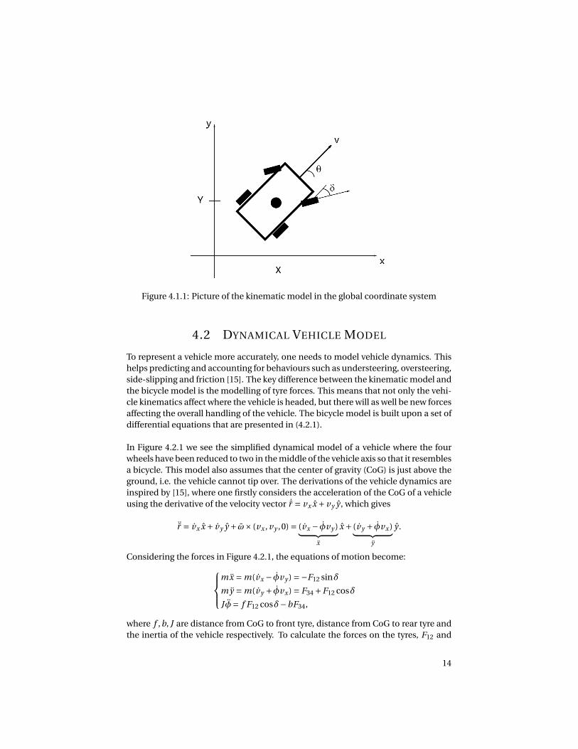
Figure 4.1.1: Picture of the kinematic model in the global coordinate system

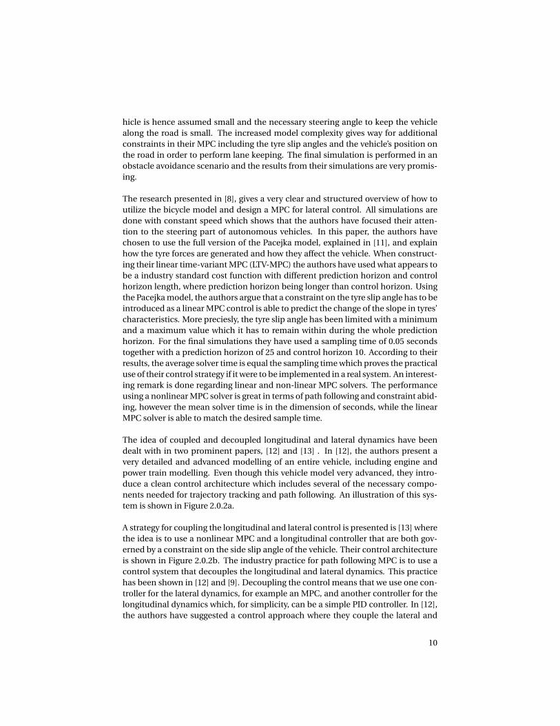
4.2 DYNAMICAL VEHICLE MODEL

To represent a vehicle more accurately, one needs to model vehicle dynamics. Thishelps predicting and accounting for behaviours such as understeering, oversteering,side-slipping and friction [15]. The key difference between the kinematic model andthe bicycle model is the modelling of tyre forces. This means that not only the vehi-cle kinematics affect where the vehicle is headed, but there will as well be new forcesaffecting the overall handling of the vehicle. The bicycle model is built upon a set ofdifferential equations that are presented in (4.2.1).

In Figure 4.2.1 we see the simplified dynamical model of a vehicle where the fourwheels have been reduced to two in the middle of the vehicle axis so that it resemblesa bicycle. This model also assumes that the center of gravity (CoG) is just above theground, i.e. the vehicle cannot tip over. The derivations of the vehicle dynamics areinspired by [15], where one firstly considers the acceleration of the CoG of a vehicleusing the derivative of the velocity vector ˙r = vx x + vy y , which gives

¨r = vx x + vy y + ω× (vx , vy ,0) = (vx − φvy )︸ ︷︷ ︸x

x + (vy + φvx )︸ ︷︷ ︸y

y .

Considering the forces in Figure 4.2.1, the equations of motion become:mx = m(vx − φvy ) =−F12 sinδ

my = m(vy + φvx ) = F34 +F12 cosδ

J φ= f F12 cosδ−bF34,

where f ,b, J are distance from CoG to front tyre, distance from CoG to rear tyre andthe inertia of the vehicle respectively. To calculate the forces on the tyres, F12 and

14

Figure 4.2.1: Picture of the bicycle model explaining acting forces, reprinted from[15].

F34, there exists a formula called "Pacejka’s Formula", or more colloquially known as"The Magic Formula" [11]. The forces are therefore usually formulated as{

Fl = fl (α, s,µ,Fz )

Fc = fc (α, s,µ,Fz ),

where Fl and Fc are the longitudinal force component on the wheel and the lateral,or cornering, force component respectively. The function fl and fc are highly non-linear and based on a semi-empirical model which depends on friction, µ, side slipangle, α, slip ratio,s and vehicle weight, Fz [10]. A plot of the non-linear behaviourof tyre forces can be seen in Figure 4.2.2.One thing to notice in Pacejka’s formula is that the tyre forces are close to linear ina small region around zero slip. When the speed of a vehicle is kept low, the slipangle and ratio stay within these bounds. Instead of using the nonlinear versionof Pacejka’s formula, one can estimate the forces with a linear function in a regionaround α = 0. This assumes that the side slip and slip angles stay relatively low,which is a fair assumption in this case where we want to control a vehicle and arenot interested in racing techniques such as drifting and sliding. Based on [15], wecan approximate the forces acting on the front and rear wheels in the bicycle modelwith: {

F12 =−C12α12

F34 =−C34α34,

15

Figure 4.2.2: The nonlinear behavior of Pacejka’s tyre formula [10].

where C12 and C34 are the cornering stiffness of the front and rear wheel respectively.The slip angles α12 and α34 are defined as:

α12 = arctan

(vy + φ f

vx

)−δ, α34 = arctan

(vy − φb

vx

).

For the coupled MPC, we will add a second control input in the form of an additionalforce on the CoG of the vehicle. The force, Fa stems from the engine for speeding upor the breaks for slowing down the vehicle as shown in Figure 4.2.3.For practical implementation reasons, the control input will be an acceleration. Us-ing newtons third law of motion, Fa = ma, yields the equations of motion:

f (z,u) =

mx = m(vx − φvy ) =−F12 sinδ+ma

my = m(vy + φvx ) = F34 +F12 cosδ

J φ= f F12 cosδ−bF34,

(4.2.1)

where the control inputs are u = [δ, a]. Putting it all together, we have six states z =[X Y θ φ vx vy

]and u = δ for the decoupled control, and u = [δ, a] for the coupled

control.

16

Figure 4.2.3: Bicycle model with added Fa force [15].

17

CHAPTER 5

VEHICLE CONTROL

5.1 SYSTEM OVERVIEW

When setting up an autonomous or automatic vehicle control system one needsmultiple layers of sensing and computational technology, and controllers that gov-ern the movement of the vehicle: lateral control and longitudinal control [4]. Thelateral controller generally controls the steering angle of the vehicle while moni-toring lateral forces that arise from cornering manoeuvres. The goal of the lateralcontroller is, simply put, to keep the vehicle on the road and to follow a path or tra-jectory. The longitudinal controller governs all the dynamics that involve the speedof the vehicle. It can be as simple as a cruise controller which keeps a vehicle at a setspeed or more advanced in terms of actively adapting the speed according to givenroad conditions [13]. The lateral and longitudinal controllers can be seen as inde-pendent systems in situations when vehicle tyre forces are small. On real roads withreal vehicles this assumption cannot be done due to factors such as road friction andwheel torque [16].

5.2 LATERAL CONTROL

The objective of the lateral controller is to output a steering angle for the vehicle. Thesteering angle is the measured angle between the vehicle’s x-axis and the directionof the steering wheels. By issuing steering angle commands, the lateral controlleraims to keep the vehicle on a reference path or reference trajectory. The lateral con-troller may also try to reduce tyre slip and excessive lateral forces when the vehicleis cornering [8, 10]. When setting up the lateral controller one needs to know whatvehicle constraints are necessary and how the control signal should be limited.

Given a situation where a vehicle is following a path, the main objective is to keepthe vehicle as close to the path as possible. Any deviations from the path are to beavoided and when the lateral controller outputs steering angles it is important thatthese control commands do keep the vehicle on the path for a close future [9]. It is

18

hence important that the lateral controller is a closed-loop control which can com-pensate for previous control errors. An important aspect of the lateral controller isthe overall vehicle stability, poor control inputs may cause the vehicle to lose lateralstability. The vehicle kinematics and dynamics are therefore important to considerin the lateral controller.

In terms of constraints, the lateral controller has to consider the physical limitationsof the vehicle. Two common limitations for the lateral controller are steering rateand maximum steering angle. The steering rate is how fast one can turn the wheelsof the vehicle and is often mechanically limited [12]. Performance wise, one wouldlike to avoid control actions that cause the vehicle to swivel on the road, and henceone tends to limit the steering rates in a conservative way [10]. On a normal pathfollowing the steering rate limitation is rarely reached while in other scenarios suchas obstacle avoidance the vehicle may operate close to the maximum steering rateof the vehicle [9]. The maximum steering angle is based on how much the wheels ofthe vehicle can turn and is often limited to 45◦.

5.3 LONGITUDINAL CONTROL

To control the speed and acceleration of a vehicle, one needs to introduce a longi-tudinal controller. From the vehicle modelling one knows that the change in speedv is given by the acceleration a. A relation on the form v = a is modelled by whatis called an integrator in field of control theory, and can be controlled by a PID-controller [17]. The acceleration of the vehicle is often constrained due to mechan-ical performance and comfort, and therefore the longitudinal controller should bedesigned with an input saturation [12]. The maximum acceleration, amax , ensures asmooth and not too aggressive acceleration while the minimum acceleration, ami n ,decides how quickly the vehicle may slow down. Usually, |amax| < |amin| given thatslowing down a vehicle is done more quickly than speeding it up and in a road safetyperspective, stopping a vehicle is more important than speeding it up [15]. The con-trol input is calculated based on reference speeds that are fed to the system and thecorresponding control action is an acceleration of the vehicle. In order to controlthe longitudinal dynamics, it is assumed that one can control the throttle responseof the vehicle, causing it to accelerate instantly. The act of accelerating the vehiclegives rise to an additional force, Fa, in the dynamic vehicle model illustrated in Fig-ure 4.2.1.

5.4 DECOUPLED CONTROL

The conventional theory on decoupling control describes how a system with mul-tiple inputs and outputs (MIMO) can have a controller that isolates the inputs andoutputs so that one input affects only one output instead of multiple. The act of do-ing so is called decoupling [18]. In vehicle control, the vehicle models have coupled

19

kinematic and dynamics which means that lateral and longitudinal dynamics mayaffect each other. Decoupled control of a vehicle means that the longitudinal andlateral dynamics of the vehicle are handled separately by two different controllers.In [16], the authors state that the dynamical forces of a vehicle must be kept low inorder to have lateral and longitudinal dynamics controlled separately. This meansthat the decoupled control may be limited by the dynamics of the vehicle.

In practice, a decoupled control strategy uses two different control approaches forthe lateral and longitudinal dynamics. Generally, the longitudinal control will befirst to optimize the acceleration and speed of the vehicle before it feeds the lateralcontroller with the current speed of the vehicle. The lateral controller then usesthe information about the speed in order to output a suitable steering angle [12]A simplified drawing of the decoupled control system is shown in Figure 5.4.1.

Figure 5.4.1: Longitudinal and lateral control diagram for the decoupled strategy.

In this thesis, the decoupled control strategy will use a PI-controller for the longitu-dinal controller and an MPC controller for the lateral control. To handle longitudinalconstraints, the PI-controller will be subject to control input saturation to avoid toolarge vehicle accelerations.

5.5 COUPLED CONTROL

The coupled control strategy attempts to benefit on the fact that the lateral and lon-gitudinal dynamics of the vehicle are coupled in both vehicle models. In the decou-pled control strategy the lateral and longitudinal controllers are separated and thelateral controller cannot send any information to the longitudinal controller, whichmay lead to unstable longitudinal control inputs[16]. In coupled control, the lateraland longitudinal control are combined into one big control problem where acceler-ation and steering angle are outputted simultaneously. The act of coupling the twocontrollers will make the control problem more complex in terms of computational

20

burden. For example, in the decoupled strategy, the longitudinal controller only hasto consider longitudinal dynamics and constraints before outputting a control ac-tion. In the coupled strategy, each longitudinal control output will also be evaluatedin terms of lateral constraints and the two controllers will be able to exchange infor-mation between them, as shown in Figure 5.5.1.

Figure 5.5.1: Longitudinal and lateral control diagram for the coupled strategy.

In this thesis, the coupled control strategy consists of one complex MPC controllerthat optimizes steering angle and acceleration while trying to abide both lateral andlongitudinal constraints. Compared to the lateral MPC in the decoupled strategy, thecoupled MPC the same lateral controller in the decoupled control, but an extendedversion to account for longitudinal control as well.

5.6 MODEL PREDICTIVE CONTROL

5.6.1 INTRODUCTION TO MPC

Model predictive control, (MPC), is an optimization based control technique thatemerged in the 1960’s in chemical processing, but today finds itself in numerous in-dustries and applications [19]. The applications are versatile and range from com-puter control on nanosecond scale to industry control and production planningwith time spans of minutes to weeks [19]. Unlike PID controllers, the MPC is basedon a formulation of an optimization problem, but unlike linear quadratic control,the MPC can handle various constraints on state and control inputs [19]. A basicMPC formulation is shown in (5.6.1).

21

minimizeui

zTHp

PzHp︸ ︷︷ ︸terminal cost

+Hp−1∑

i=1zT

i Qzi +uTi Rui

subject to z0 = z(0) measurement

zi+1 = Azi +Bui linear system model

Czi +Dui ≤ b constraints

R º 0,Q º 0 performance weights,

(5.6.1)

where ui ={

u0,u1, . . . ,uH p−1}

is a sequence of optimal control inputs that minimizesthe cost function, and z is the state of the system we are trying to control. The sum-mation is done over a number of iterations, Hp , called horizon, which means thatthe MPC does not only calculate the next control input but also plans ahead for fu-ture control inputs by trying to predict the behaviour of the system.

The four core parts of an MPC are its cost function, the system model, the con-straints and the state measurements. These measurements can come from eithera state observer of physical measurements. The cost function has three parameters,or weight matrices, Q, R and P. These matrices are used to penalize the states andcontrol inputs during the optimization and tuning them is essential for the perfor-mance of an MPC. The Q matrix is most commonly a diagonal matrix of size (n ×n)and the R matrix is of size (m ×m) where n equals the number of states and m thenumber of control inputs.

The matrices C and D help select the states and control inputs that are to be con-strained by b. A common use of D is to set limits on the control signal u on the formu ∈ [umin,umax]. The matrix P which appears together with the last predicted state,or terminal state, zHp is called terminal state cost. The purpose of the terminal costis to emphasize the importance of the final state to reach the optimal state. This isnormally done by designing the elements of P so that that they are larger than theelements of Q.

5.6.2 MPC FOR TRACKING

The MPC formulated in (5.6.1) is a linear MPC, used when one wants to bring a sys-tem to the origin, but one can can rewrite (5.6.1) so that it can track a constant refer-ence r 6= 0. Using theory from [20], we assume that there exists a state zs and controlinput us that keeps the system at reference r as in the linear time-invariant (LTI)system (5.6.2). {

zt+1 = Azs +Bus = zs

y = Czs = r.(5.6.2)

The "s" stands for "steady state", but for our application with tracking and path fol-lowing, we will use the notation is zref and uref. What we now want to minimize isnot z but (z−zref) and (u−uref). This is suitably done by introducing two new states:

22

z = (z−zref) and u = (u−uref). We can now rewrite (5.6.1) to adjust for the new vari-ables.

minimizeu

zTHp

PzHp +Hp−1∑

i=1zT

i Qzi + uTi Rui

subject to z0 = z(0)

zi = (zi −zref)

ui = (ui −uref)

zi+1 = Azi +Bui

Czi +Dui ≤ b.

(5.6.3)

The optimal control input u∗ is taken from u∗ = u∗+uref. The value of zref can betaken directly from y = C zref = r , meanwhile uref can be acquired in a few differentways. The more analytical way of doing it is knowing the reference r that we want totrack, and then find the steady state zref through C zref = r . To remain in steady state,there has to exist a control input uref which keeps us in that state when time tendsto infinity.

From (5.6.2) we get that zref = Azref +Buref, and from here we can solve for uref byconstructing the inverse of B and writing everything as

uref = B−1(I−A)zref. (5.6.4)

Note however that B−1 in (5.6.4) is only valid if B is square and its determinant iswell defined and not zero [21]. In practical applications, when this is not the case,the analytical pseudo-inverse can be used to approximate uref. In later chapters ofthis thesis it will be shown that one can achieve good tracking with suboptimal uref

if you tune Q and R cleverly. In our path following scenario, the information fromthe waypoints prove useful for determining the steady state control input uref. Dis-cretizing θ in (4.1.1) yields

θt+1 = θt + vTs

Ltan(δ)

and from this we can find the reference steering angle uref = δref that will bring ourvehicle to zref by solving for δref

δs = arctan

(L

Ts v(θi+1 −θi )

)

5.6.3 MPC FOR PATH FOLLOWING

In this thesis we aim to use an MPC tracking algorithm, but unlike (5.6.2) we are notinterested in tracking one constant reference, but rather a time-varying reference.As the vehicle moves along the path it needs multiple references to follow to ensurethat the vehicle maintains itself on the path. This puts a lot of demand on the ref-erences and the MPC tracking algorithm. As the vehicle travels along the path the

23

waypoint update algorithm has to work in real-time to supply the MPC with refer-ence points to track and if it fails to deliver valid references the path following mayfail.

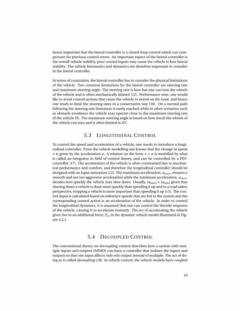
Figure 5.6.1: MPC path following with waypoints and reachable sets.

To solve this problem we introduce multiple references in control horizon so thatthe vehicle tracks a new reference every iteration. Using this algorithm, one needsto update zref and uref at each sampling time. Formally, this changes our referencecontrol input to uref = (us0 ,us1 , . . . ,usHp−1 ,usHp

) as well as our reference states be-come zref = (zs0 ,zs1 , . . . ,zsHp−1 ,zsHp

). This method ensures that the vehicle tracks thereference well while avoiding to deviate from the path assuming the reference arereachable and valid for the vehicle, see more in section 6.2.

A general path following case is depicted in Figure 5.6.1 where the current state z0

is the small black circle and ahead of it are four waypoints. Around each waypointis a larger circle that signifies the points where the MPC is allowed to be, the reach-able set. These sets have a radius of ε and the state constraints of the MPC will tryto ensure that the MPC is contained within these sets. Each waypoint has a corre-sponding iteration number i which means that after the first iteration, the states willbe somewhere in set i = 1, in iteration two it will be in set i = 2 and so on. The eu-clidean distance between the waypoints is chosen so that the vehicle can reach eachwaypoint with its current velocity. The rate of change in control input u is limited by

24

setting a maximum control input change between iterations, and maximum controlinput is constrained using absolute value of u.

The final MPC formulation for the lateral controller for solving the path following inFigure 5.6.1 is summarized in equation (5.6.5).

minimizeu

zTHp

PzHp +Hp−1∑

i=1zT

i Qzi +Hc∑i=0

uTi Rui

subject to z0 = z(0)

zi = (zi −zrefi )

ui = (ui −urefi )

zi+1 = Ai zi +Bi ui

|zi | ≤ ε|ui+1 −ui | ≤∆u

|ui | ≤ umax .

(5.6.5)

5.6.4 LINEAR MPC

The vehicle models presented in Section 4 contain nonlinear terms and the bicy-cle model in (4.2.1) is highly nonlinear after introducing tyre forces [15]. There arenonlinear optimization solvers capable of solving the MPC problems but they areall very time consuming [22]. Nonlinear optimization solvers have been used forMPC and vehicle path following, but averaging 2 - 3 seconds for each iteration whenthe solving time should equal the sampling time between 0.01 and 0.05 seconds, thenonlinear approach is often deemed unsuitable [8].

A possible approach is to use a linear MPC approach which in this application of ve-hicle path following means that one has to linearize the vehicle models before solv-ing the MPC. The idea of linearizing a nonlinear system is to find a correspondinglinear system that behaves roughly the same as the original. In path and trajectoryfollowing, the nonlinear model of the vehicle changes too much during the horizonwhich means that one has to linearize at each sample time [8]. From equation (5.6.5)we can rewrite the system model with a new notation:

zi+1|i = Ai zi |i +Bi ui |i (5.6.6)

Since the vehicle model will be linearized for each iteration, the A and B matriceswill receive a new notation to show which iteration they belong to. The notationzi+1|i means the state z at iteration i +1, based on predictions from iteration i .

Given a system on the form z = f (z,u), we need to calculate two matrices, A and B,so that we can write the system as (5.6.6). Since linearisation is only valid in smallregions, we need to linearise around every point we want the vehicle to pass. Wedenote such a point (zref,uref). Given that zi+1|i = zi + f (zi |i ,ui |i := g (zi |i ,ui |i ), we getthat:

25

Ai = ∂g (zi ,ui )

∂z

∣∣∣ zi=zrefiui=urefi

Bi = ∂g (zi ,ui )

∂u

∣∣∣ zi=zrefiui=urefi

.

What we now have is actually a system on the form:

zi+1|i −zrefi+1|i = Ai (zi −zrefi )+Bi (ui −urefi ),

since we want to investigate the behaviour around (zi ,ui ). This will prove to beuseful in the case of tracking MPC where the system model is written using tilde-formulation where z = z−zref. For each iteration and each horizon step, the systemmodel needs to be relinearized in order to have as good as possible approximation.

In the case of the kinematic vehicle model given in (4.1.1), where zt+1 = g (z,u), alinearization around zref = [xs ys θs v] and uref = [δs ] would yield:

A = ∂g (z,u)

∂z=

1 0 −vs sinθs cosθs

0 1 vs cosθs sinθs

0 0 1 tanδsL

0 0 0 1

B = ∂g (z,u)

∂u

0 00 00 vs

L sec2δs

0 1

.

5.6.5 TURN MPC INTO QUADRATIC PROGRAMMING

The MPC problem stated in (5.6.5) can be solved by transforming the MPC formula-tion into QP [14]. Given a discrete-time system model

zi+1|i = Ai |i zi +Bi |i ui |i , (5.6.7)

and a standard MPC formulation as the one given in (5.6.1), the states of the systemwill be predicted up till the horizon end Hp , where

z(Hp |i ) = A(Hp −1|i )z(Hp −1|i )+B(Hp −1|i )u(Hp −1|i ).

This approach will lead to Hp amount of states and inputs which would mean thatone needs to solve for Hp control inputs and predict (Hp ×n) states [5]. Rewritingthis, we can create a QP problem which only depends on the initial state z0 and con-trol inputs u.

In order to track how the states change during the MPC iterations, we introduce twovectors:

zi+1|i =

zi+1|i

z(i +2|i )...

z(i +Hp |i )

ui+1|i =

ui+1|i

u(i +2|i )...

u(i +Hp |i ),

,

using these two vectors we can write one big system that accounts for the evolutionsof the MPC iterations over the horizon, hence create something on the form

26

zi+1|i = Ai |i zi |i + Bi |i ui |i .

The matrix Ai |i has one column and Hp number of rows, with a product sum ofAi |i ,Ai+1|i , ...,A(i + Hp |i ) matrices. The matrix Bi |i is a lower triangular matrix con-taining both A and B matrices. The complete structure of the two matrices, as seenin [5] is

Ai |i =

Ai |i

Ai+1|i Ai |i...

α(i ,1,0)

Bi |i

Bi |i 0 0 ... 0Ai |i Bi |i Bi+1|i 0 ... 0

......

.... . .

...

α(i ,2,1)Bi |i α(i ,2,2)Bi+1|i. . . ... 0

α(i ,1,0)Bi |i α(i ,1,2)B(i −1|i ) ... ... B(i +Hp −1|i )

,

where α(i , j , l ) is defined as

α(i , j , l ) =N− j∏i=l

A(i + i |i ). (5.6.8)

Constructing new matrices Q = diag(Q, ...,Q) and R = diag(R, ...,R) we can rewritethe cost function in (5.6.5)

Φi = zT (i +1)Qz(i +1)+ uTi Rui . (5.6.9)

The general QP problem is aimed to solve a problem on the following form [22]:

minimizeu

1

2uT Hu+ fT u+d

subject to Au ≤ b.(5.6.10)

For the MPC formulated as a QP, one wishes to solve for the control inputs u thatminimizes the cost function in (5.6.5). Changing the variable u in (5.6.10) with con-trol input u we get a QP cost function on the form:

φi = 1

2uT Hu +cT u +d.

To construct the matrices H, f and d we look at (5.6.9) and use that z(i +1) = Ai |i z+Bi |i u.From this we collect the quadratic and linear u terms as well as the constantterm not containing u and then we identify from these H,c and d, presented in(5.6.11).

27

Hi = 2

(BT

i |i QBi |i + R)

fi = 2Bi |i QAi |i zi |idi = Ai |i zi |i QAi |i zi |i .

(5.6.11)

Now that the optimization problem and the cost function have been constructed,the next items to add are the state and input constraints used in MPC. Since thevariable one wishes to optimize in the MPC is u, the state constraints are rewrittenas Du ≤ c. Depending on the amount of control inputs m, the size of u will be onecolumn and m × Hp rows. What we wish to constrain with Du ≤ c is umi n ≤ ui ≤umax . To put all this into matrix form, we use the same method as in [5] wherethey construct D as a diagonal matrix with first half of diagonal being equal to 1 andthe second part equal to −1. Since ui = ui −urefi , we need to compensate for thereference inputs in the d vector. The d vector is then upper half consisting of umax −uref values and lower half umi n+uref values so that one gets u−uref ≤ umax−uref and−(u −uref) ≤ umi n +uref. Note that even if umi n < 0, when constructing d one has touse the absolute values of umax and umi n as the sign shift in D makes sure that theconstraints are correctly represented, as shown in (5.6.12).

D =

1 0 0 00 1 0 00 0 −1 00 0 0 −1

c =

amax −aref

δmax −δref

−ami n +aref

−δmi n +δref

. (5.6.12)

If one wishes to impose a constraint on the vehicle states z, it is necessary to writethe constraint so that it is imposed on u since it is the optimization variable. As-sume we wish to constrain the vehicle in terms of deviation from the reference path,||zi || ≤ ε ∀i , we have to rewrite this in terms of u. Using the fact that z(i + 1) =[z(i +1)z(i +2) . . . z(N +1)] and z(i +1) = Az+ Bi ui we get:

Dz(i +1) ≤ c ⇔ D(Az+ Bi ui

)≤ c ⇔ Dui ≤ c, (5.6.13)

where D is the same as in (5.6.12) and

c = B−1i

(ε− Ai zi

).

5.6.6 TUNING

In standard PID control theory there are several methods for tuning the controllerin order to affect its performance [17]. In PID control there are gains and tuningparameters which will effectively change its behaviour which makes it highly cus-tomizable and is partly one of the reasons why it has been in such great use in theindustry [18]. In the case of MPC, which is a mathematical optimization problem,the tuning is done slightly differently and most of it comes down to the cost functionand the optimization constraints [20].

28

Taking a look at the cost function, there are three matrices involved that are nei-ther states nor control inputs: Q, R and P. Starting with the Q matrix, it is used incombination with the system states and in the cost function they together create aquadratic cost zT Qz. What Q effectively does is penalizing the solver for any devi-ations in the states [19]. If one wants to keep all three states equally close to theirreferences, the weights would be chosen to be identical. However, if one or twostates are more important to track than the other, the weights for these states wouldbe greater than those for the less important. Practically this means that any devia-tion in the more important states will be greater penalized, leading to the MPC willtry to find solutions which minimize the deviation in the important states while thedeviation in the less important states is allowed to be larger. The size of the weightshave to be in relation of the quantity it is penalizing. For example, penalizing metersand radians with the same weight means that one meter path deviation is equallypenalized as one radian orientation deviation.

In vehicle path following, the x and y coordinates are deemed the most importantstates as one wants to stay on the road at all times [8]. The weights for these twostates are then often the largest. The orientation of the vehicle is not as equally im-portant since tyre slip angle and the effective heading angle of the vehicle might notbe equal to the physical orientation.

The R matrix appears together with the u and serves as a weight matrix for the con-trol inputs. In the tilde formulation it penalizes deviations from the reference con-trol inputs and states. As in the case of the Q matrix, the elements of R are chosen sothat the control inputs can penalized differently. Since the cost function summarisesthe penalties of the states and control inputs, the interaction between Q and R is ofequal importance. If the elements of Q is greater than those of R it would mean thatdeviations in states are more important to avoid and the control strategy would beto minimize the states even if it would mean having large deviations in control in-puts. Therefore, the elements of R are usually chosen to be smaller than those of Qin the lateral controller [12].

The terminal cost matrix P has a very dominant effect on the MPC, even tough itonly penalizes one instance of the states, namely the terminal state zHp [19]. Sincethe MPC predicts over a horizon, the iterations between the initial state z0 and the fi-nal state zHp can be seen as steps on a path from the starting point to a goal. In stan-dard non-path following MPC, what one is interested in is not as much how it travelsto the goal but rather that it reaches that point and does it well. The elements of Pare almost always greater than those of Q to emphasize that the final state is moreimportant than the path to it. In path following MPC, the path is equally importantto the goal and the terminal cost serves as a stabilizing and recovering weight whichis discussed more in Section 6.6.

29

5.6.7 COUPLED PATH FOLLOWING MPC

In our specific case, coupled control means that there will be one MPC controllerthat will be responsible for two control inputs, steering angle and acceleration, ateach iteration. Looking at the bicycle model shown in (4.2.1), the steering angle hasa direct effect on the tire slip angle which in itself affects the lateral, longitudinal andyaw rate of the vehicle. These three together affect the position and orientation ofthe vehicle. The control inputs affect each other and each state of the vehicle, andthe idea of letting one MPC optimize both inputs is to better predict the evolutionthe states of the vehicle and improve stability.

The suggested MPC formulation for coupled control will include constraints on bothcontrol inputs and the states for both the kinematic and dynamic models. The costfunction of the coupled MPC will remain the same as in the lateral control presentedin (5.6.5), but, with more states to track, the matrices Q,P and R will have additionalelements. The terminal cost matrix P is tuned in accordance with the theory statedin Section 5.6.6 and will follow the same structure as Q but with larger elements. TheR matrix for the coupled system will be R = diag(r1,r2) where tracking reference ac-celerations and steering angles are of similar importance.

For the bicycle model there are two more states to consider into the cost function,namely φ and vy . This adds two more elements in Q and P but they can both beignored and set to either zero or one. The reason for this is that even though φ andvy affect the handling of the vehicle, one can still perform path following withouttracking these two variables. This also means that we do not need to generate anyreferences for these states.

The control strategy used here therefore suggests that one does not focus on theevolution of φ and vy . One can however add constraints on these two in terms ofdifferent stability criteria. A suggested way of creating references for vy is to setvy,r,i = vy,i−1, or in words the future reference of the lateral speed is the lateral speedfrom previous iteration. This way, vy is allowed to grow but very quick or suddengrowths will be penalized and hopefully avoided.

5.7 SPEED PROFILING

With the strategies suggested in section 5.6.7 we have now introduced a second con-trol input in form of an accelerating force which acts upon the vehicle and effectivelyalters its speed. To find the optimal acceleration we introduce an additional blockin our system called speed profiler. The goal of this block is to produce an optimalreference speed vref for each point on the path [12]. The definition of vref will fromhere on be equal to the maximum speed a vehicle can have without slipping on theroad surface [12]. To find vref one utilizes information about the road and vehicleconditions at the given time. A simple formula for determining the maximum speedon a road is given by

30

vmax =√

gµ

ρr, (5.7.1)

where g ,µ and ρr are gravity, friction coefficient and road curvature respectively. In[12] the authors use an extended formula which introduces road chamber angle, φr ,which explains how much the road banks, or, how level the road is. For the applica-tions of this thesis, all of the tested roads have zero bank and hence equation (5.7.1)suffices. The curvature ρr is defined as 1/r where r is the radius of the road curve.According to [23], the curvature can be estimated using only three points one a road,pi−1, pi and pi+1. Constructing two vectors v1 = pi −pi−1, v2 = pi+1−pi and the cur-vature at point pi is given by

ρr,i =2sin

(θ2

)p||v1|| · ||v2||

with θ = arccos

(v1

||v1||· v2

||v2||)

. (5.7.2)

Using (5.7.1) and (5.7.2) one can now determine vmax for each waypoint on the path.The formula in (5.7.1) will diverge when ρr → 0, and hence straight roads will be lim-ited to a predetermined maximum value.

Using this information one can create the speed profile for any road. Using the pathin Figure 5.7.1a, plotting vmax for each point of the path results in the speed profilein Figure 5.7.1b. Here, vmax = 10 m/s on the straight segments of the path.

(a) Path for the speed profiling.

0 500 1000 1500 20005

6

7

8

9

10

11

12

Waypoint number

v max

Speed Profile

(b) Speed profile for the path in Figure 5.7.1a.

Figure 5.7.1: Two different control hierarchies.

Using the speed profile we can feed the reference speeds to the longitudinal con-troller and the system tries to follow the path as well as adapt its speed during thedrive. An issue with the speed profile in 5.7.1b is that if the speed of the vehiclebefore it enters the corner, entry speed, is much larger than the maximum speed al-lowed inside the corner, the deceleration needed to suit the new vmax might be toolarge for the vehicle to handle. A safe limit for deceleration is set to amax =−1 m/s2.

31

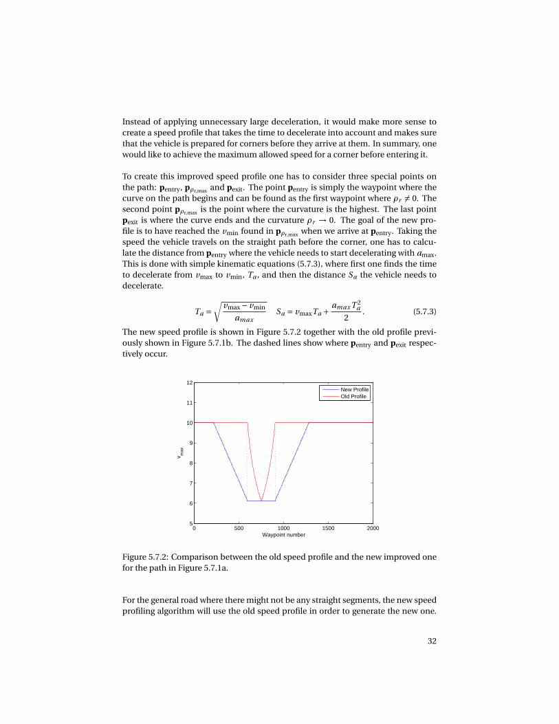
Instead of applying unnecessary large deceleration, it would make more sense tocreate a speed profile that takes the time to decelerate into account and makes surethat the vehicle is prepared for corners before they arrive at them. In summary, onewould like to achieve the maximum allowed speed for a corner before entering it.

To create this improved speed profile one has to consider three special points onthe path: pentry, pρr,max and pexit. The point pentry is simply the waypoint where thecurve on the path begins and can be found as the first waypoint where ρr 6= 0. Thesecond point pρr,max is the point where the curvature is the highest. The last pointpexit is where the curve ends and the curvature ρr → 0. The goal of the new pro-file is to have reached the vmin found in pρr,max when we arrive at pentry. Taking thespeed the vehicle travels on the straight path before the corner, one has to calcu-late the distance from pentry where the vehicle needs to start decelerating with amax.This is done with simple kinematic equations (5.7.3), where first one finds the timeto decelerate from vmax to vmin, Ta , and then the distance Sa the vehicle needs todecelerate.

Ta =√

vmax − vmin

amaxSa = vmaxTa +

amax T 2a

2. (5.7.3)

The new speed profile is shown in Figure 5.7.2 together with the old profile previ-ously shown in Figure 5.7.1b. The dashed lines show where pentry and pexit respec-tively occur.

0 500 1000 1500 20005

6

7

8

9

10

11

12

Waypoint number

v max

New ProfileOld Profile

Figure 5.7.2: Comparison between the old speed profile and the new improved onefor the path in Figure 5.7.1a.

For the general road where there might not be any straight segments, the new speedprofiling algorithm will use the old speed profile in order to generate the new one.

32

Knowing the waypoint spacing, one can measure the distance between the last pointof maximum speed and the point with the slowest speed. From this, the speed pro-filer can calculate the appropriate point to start decelerating in order to bring thevehicle speed down to a minimum well before entering the road segment with low-est allowed top speed.

33

CHAPTER 6

SIMULATION SETUP

In this section the different controllers and the complete system is evaluated usinga simulation environment in MATLAB. The primary goal is to evaluate the differentcontrollers separately at first using different tuning options and performance mea-surements. In the last part of this section all controllers that have been tested on thedynamical bicycle model vehicle will be compared in a final test in order to find datawhich will be used in the discussion and ultimately serve as base for answering thequestions posed in the problem formulation in Section 3. The complete system thatwill be used in the simulation and evaluation is a combination of all systems men-tioned in Section 5. An overview of the full system is given in Section 6.1 and shownin Figure 6.1.1.

6.1 SYSTEM OVERVIEW

The simulation setup is shown in Figure 6.1.1. The closed loop system consistsof three major blocks: path_generator(), controller() and vehicle(). Thefirst block path_generator() will take a continuous version of the path and out-put a discretized version in form of a set of waypoints W. This set is stored in thecomputer and is constantly used through the path following. The second blockcontroller() can be broken down into three smaller blocks: find_waypoints(),find_input() and MPC(). The first block find_waypoints() will use the currentposition of the vehicle and the set of waypoints in order to select the waypoints thatwill be used for the next iterations. The find_input() block will use these way-points to create reference control inputs which are then passed down to the MPC()

block which performs the actual optimization problem and outputs control inputs.The MPC() block uses the reference waypoints to first linearize the system aroundeach point. Finally, it solves the MPC problem and the control inputs are fed tothe block vehicle(). The updated states of the vehicle are then fed back into thecontroller() and the loop is closed. For the simulations with longitudinal control,the path_generator()will include a speed profile element which together with theset of waypoints store the optimal speed for the entire path. These speed profile val-

34

ues are then passed along with the discrete path to the controller() block.

Figure 6.1.1: An overview of the control system used for path following.

6.2 WAYPOINTING - CREATING THE REFERENCES

In a 2D space one can track a vehicle using two coordinates x, y and an orientationθ which is described by the vehicle models in Section 4. To perform path followingthe vehicle needs reference points to follow, or waypoints. The waypoints describe aposition in the 2D space as well as an orientation. A waypoint is henceforth definedas a vector zref containing at least information about x, y and θ, and any path in thisspace can be described using a vector of waypoints W. When constructing W from acontinuous path, it is built using multiple discrete waypoints

[zref0 ,zref1 , ...,zrefN

].

Given an MPC horizon of Hp , we would need to input at least Hp waypoints which isordered as zref = [zref0 ,zref1 ,zref2 . . .zrefHp−1 ,zrefHp

]. The waypoint zref0 is the waypointclosest to the initial state of the vehicle z(0). This first waypoint zref1 is defined asthe first reachable waypoint when moving from the initial state z(0), which is foundusing Ts and v . The vehicle will travel Ts v meters per sampling time, hence the eu-clidean distance between zref0 and zref1 have to equal to this. The waypoint in W thatbest matches this criteria is chosen as w1. The following waypoint for the MPC hori-zon is chosen in the same fashion using the same speed and sampling time.

After choosing appropriate waypoints for the path following, the MPC will then tryand minimize z for each iteration and bring the vehicle state zi close to its respectivewaypoints zrefi . Since the waypoints are highly dependent on the vehicle’s currentstate, they have to be calculated online at each sampling time. The algorithm forfinding appropriate waypoints is shown in Algorithm 1.

35

Data: z(0),v ,Ts ,Hp ,WResult: Extract Hp number of waypointsFind zref0 ∈ W such that ||z(0)−zref0 || is minimized. ;Find Ss using Ss = vTs ;while i ≤ Hp do

Choose zrefi ∈ W such that;||zrefi −zrefi−1 ||−Ss is minimized;i ++;

endReturn zref = [zref0 , ...,zrefHp

];Algorithm 1: Find waypoints

6.3 SIMULATION PATH

The path where the controllers are tested on is a long > 180 degree corner that hasa 30 meter straight leading into the curve and a 30 meter straight leading out of it.The road friction is set to µ = 0.7 which is less slippery than µ = 0.3 used in [9], butmore than µ= 1 used in [13]. The path along with its boundaries is showed in Figure6.3.1. The maximum speed of the path is chosen to 10m/s but is considerably lowerinside the corner. The dashed line shows the center line of the road which servesthe purpose of path for the path following. The width of the road is 2 meters and ifa controller fails to keep the vehicle within these boundaries the controller will begiven a failure status in the later simulation tables. However it is allowed to deviatefrom the center line and the amount it deviates will be presented in the performancetables.

6.4 PERFORMANCE MEASUREMENT AND TUNING

In this section of the thesis a thorough presentation of the different controllers thatwere developed is done and each one is evaluated through simulations in MATLAB.To evaluate each control strategy and their respective controllers, several perfor-mance numbers summarized in Table 6.4.1 will be used.

Table 6.4.1: List of used performance indicators

Symbol Name DescriptionTsol MPC solver time Average time to solve the full MPC problemudev Input deviations How much does u∗ deviate from uref

zmax Max z deviation The maximum deviation from the path∆z Average z deviation Measures how well the vehicle is able to

match the waypoints.

36

Figure 6.3.1: The corner used for the simulation together with its boundaries andthe center path.

The Tsol indicator measures how long the computer takes to solve the MPC prob-lem. The tasks included in Tsol are linearizing the system for each waypoint, cal-culating optimal speed, acceleration and steering angle, applying the longitudinalcontroller and/or solve the full MPC. In [6, 7, 8, 10] the authors have used a sam-pling time of Ts = 0.05 seconds, while [14] has used Ts = 0.01 seconds. The paperswith longer sampling time usually have more complex dynamics than the resultshere, and hence Ts = 0.01 seconds will be used as a benchmark. For the MPC to bepractical, Tsol ≤ Ts or else one may end up with suboptimal solutions [10].

The waypoint based indicators are used to show how well the controllers follow thereference path. The indicator zmax presents the largest deviations from the path thatthe vehicle has done during the simulation. A zmax ≤ 0.5 meters is deemed accept-able. The second indicator ∆z is a measurement of average waypoint deviation, andmeasured as average centimeter deviation per waypoint.

The last indicator udev measures the average deviation in control input from controlreference. Although not being a critical performance indicator, it shows how muchthe controller has to adjust the control inputs from the references in order to per-form path following.

37

6.5 MPC SOLVER EVALUATION

To solve the quadratic programming and MPC problems constructed in this thesis,a numerical solver tool is necessary to use. Three different solvers are tested: MAT-LAB and its function quadprog, CVXGEN QP solver and CVXGEN MPC solver. TheCVXGEN solvers are created by professor Stephen Boyd and Ph.D candidate JacobMattingley. The QP solver is explained in their paper [24] and it can be used for mul-tiple types of convex optimization including quadratic programming and MPC. Thedetails for the MPC specific solver can be found in [25].

The first two solvers are quadratic programming solvers which require the user torewrite the MPC problem into a QP problem. The third solver is a MPC solver anddoes not require the user to rewrite the MPC into QP which simplifies parts of theimplementation. For the QP solvers, the MPC has to be written on the form givenin equation (5.6.11). The aim is to optimize a sequence of control inputs u. At eachsampling time the system is linearised around zref and the matrices A and B are con-structed and then fed to the solver which outputs a Hp long sequence of optimalcontrol inputs. The first input u0 is given to the simulation of the system which up-dates the vehicle position, and the future state predictions from the MPC are plot-ted. Table 6.5.1 collects all the information about different MATLAB simulationsperformed on the kinematic system. Performance numbers as well as simulationparameters such as sampling time and speed are noted.

The built-in QP solver in MATLAB is easy to use but is a relatively slow QP solver. TheQP solver from CVXGEN is documented to be faster than MATLAB’s quadprog butrequires the user to compile the solver source code each time the MPC is changed.The CVXGEN MPC tool is a solver for MPC problems which does not require havingto manually rewrite the MPC into a QP. The major upside to this is that one can eas-ily add, remove or modify constraints without having to rewrite the matrices D andd as it was done in Section 5.6.5.

The results from the solver testing are shown in Table 6.5.1, which concludes that theCVXGEN solvers are faster than MATLAB’s solver. The CVXGEN MPC solver is onlyslightly slower than its QP solver, but the more simple implementation has made theCVXGEN MPC solver the chosen solver for this thesis.

Table 6.5.1: Simulations using kinematic MPC on a kinematic vehicle model andcruise controller at v = 10 m/s

Solver ∆z [cm] zmax [cm] Tsol [ms] Ts [ms] udev [◦]QuadProg 0 0 10.5 10 0CVXGEN QP 0 0 8.0 10 0CVXGEN MPC 0 0 8.8 10 0

38

6.6 TUNING THE CONTROLLERS

The tuning of the controllers have taken inspiration from [6, 7, 10], among many,but it is also much trial-and-error. An important note on tuning is the significanceof the terminal cost matrix P. Given the situation that our vehicle starts outside ofthe path and it is now trying to get back on it. With an MPC where P = Q, every statein the horizon is equally important and the solution that brings the vehicle closest tothe waypoints will be sought after. To improve the performance of the MPC, the ma-trix P can be tuned differently. The elements of P matrix can be greater than thoseof Q, meaning that the last waypoint to follow is more important than the previousones. This is especially useful in situations when the vehicle has been deviating fromthe path already. The terminal cost will force the vehicle to steer in a way that thelast waypoint is reached and the proceeding waypoints do not have to be strictlyfollowed. In Figure 6.6.1, the vehicle is starting 0.5 meters south of the path and istrying to re-enter the path. The x and y axes are scaled differently to easier see theeffect. The dashed line shows how the vehicle travels when P = Q and the dotteddashed line uses P > Q. The latter tuning strategy reduces the oscillations and con-verges more quickly towards the path compared to the other tuning.

10 15 20 25 30−1.5

−1

−0.5

0

0.5

1

x−position [m]

y−po

sitio

n [m

]

PathVehicle P > QVehicle P = Q

Figure 6.6.1: Comparison of using terminal cost versus not using it.

39

CHAPTER 7

SIMULATION RESULTS

7.1 DECOUPLED CONTROL

7.1.1 KINEMATIC DECOUPLED MPC ON KINEMATIC MODEL

The results in Section 6.5 show that a kinematic MPC with constant speed control-ling a kinematic vehicle model leads to near perfect trajectory following, this sec-tion will demonstrate the principles of decoupled lateral and longitudinal control.From henceforth the CVXGEN MPC solver will be used. The longitudinal controllerwill be a PI-controller which is described in Section 5.3. The longitudinal controllerwill have control input saturations in order to use slightly more realistic dynamicsin terms of breaking and acceleration.The acceleration limit, deceleration limit andcontroller gain is set to amax = 1 m/s2, amin =−5 m/s2 and KP = 3, KI = 1.

The simulation is performed using the more aggressive speed profile, while the newspeed profile is tested separately in Section 7.4. The vehicle model used has fourstates and one control input, and the tuning parameters for lateral controller is shownin Table 7.1.1

Table 7.1.1: Tuning and limits of lateral controller

Q R P δmax , δmi n ∆δmax

[100,100,1,0] 10 [500,500,5,0] ±50◦ 40◦/s

As expected with similar models in the MPC and on the simulated vehicle, one achievegreat path following in all three cases. The reason that the deviations arise is that thelimits on the longitudinal controller causes the speed of the vehicle to not be opti-mal in the corner. If one investigates the plots in Figure 7.1.1, it is possible to seethat the longitudinal controller cannot react to the reference speed change withoutbreaking the acceleration limit and is thus always lagging behind the reference. Thesteering angle input follows the reference pretty accurately apart from a few control

40

reference jumps.

0 10 20 30 40 50 60 70 805

6

7

8

9

10

11

12

Distance [m]

Spe

ed [m

/s]

Vehicle SpeedSpeed Reference

0 10 20 30 40 50 60 70 80−5

0

5

10

15

20

Distance [m]

Ste

erin

g A

ngle

[deg

]

Control InputReference Input

Figure 7.1.1: Vehicle speed and speed reference (left) and steering angle control in-put and input reference (right).

An important thing to notice in this simulation is that the solver time is well belowthe stipulated sampling time of Ts = 0.01 seconds. Hence, using such a small hori-zon of Hp = 10 will not fully utilize the capacity of the processor of the computer.This means that there is room to increase the complexity of the MPC which can bedone by either adding constraints to the system or simply increase the horizon.

The control strategy was re-simulated with increased horizon and compared to itsshort horizon equivalent. The Hp = 30 horizon proved to have slightly too long solv-ing time and a third tuning with Hp = 25 was also tested. The result and comparisonis shown in Table 7.1.2.

Table 7.1.2: Performance comparison for different horizons.

Hp ∆z[cm] zmax[cm] Tsol[ms] udev[◦]10 0.7 10.3 2.4 0.225 0.3 1.1 9.4 0.230 0.3 1.2 11.2 0.2

The increased horizon reduces the average waypoint deviation by 50% and reducesthe maximum deviation from 10cm to roughly 1 cm. Since Hp = 25 has a sufficientsolver time it will be used as standard for the kinematic modelled MPC.

41

7.1.2 KINEMATIC DECOUPLED MPC ON DYNAMIC MODEL

After showing how using identical models in simulations and in the MPC yields nearperfect tracking with both constant speed and decoupled longitudinal controller,one would now like to investigate how the kinematic MPC controllers handle a sys-tem governed by a more complex dynamical bicycle model. The following simula-tions are also important in the sense that the kinematic model in (4.1.1) is a simpli-fied version of the dynamical bicycle model in (4.2.1). An example of a simplificationdone is the assumption that in the kinematic equations there exists no lateral speedvy , and what we want to find out here is if the kinematic MPC can control the dy-namical system. The two different models are more equal if vy is kept low and otherdynamics are within some small bounded region.

The controllers used in this simulation are the same as in Section 7.1.1 and the sim-ulation is performed on the bicycle model presented in (4.2.1). The performancenumbers of the three simulations are summarized in Table 7.1.3.

Table 7.1.3: Performance indicators for kinematic decoupled control with Hp = 25

∆z[cm] zmax[cm] Tsol[ms] udev[◦]12.4 35.2 9.6 0.5

The reference input values us are collected from a kinematic vehicle model and forc-ing the MPC to follow these references simply displays that the reference values arenot optimal for the simulated vehicle. The control input deviations are larger for thissetup compared to the ones in Table 7.1.2, which is expected as the MPC has to workharder in order to follow the path.

7.1.3 DYNAMIC LATERAL MPC ON DYNAMIC MODEL

The next MPC to investigate is the one based on the dynamic model presented in(4.2.1). Firstly, the lateral controller will be constructed and tuned for constant speedand a decoupled and coupled version will be tested. The six state vehicle model re-quires extra tuning parameters for the MPC as well as extended matrices Q,R,P inthe cost function. Similar to the kinematic based MPC controllers, the bicycle modelbased MPC will track position and orientation states and the importance of thesestates are the same in both kinematic and dynamic cases. The major difference isthat the dynamic model distinguishes the velocity from a simple v in the kinematicmodel to component speeds vx and vy in the bicycle model which are tracked sep-arately. The change is vehicle orientation φ = vφ is now a state the MPC can workwith. However, for our path following these states are not tracked but they are con-strained.

When tuning the lateral MPC a couple of assumptions regarding the evolution of thestates are made. The speed vx is tracked and deviations from calculated reference

42

0 10 20 30 40 50 60 70 805

6

7

8

9

10

11

12

Distance [m]

Spe

ed [m

/s]

Vehicle SpeedSpeed Reference

0 10 20 30 40 50 60 70 80−2

0

2

4

6

8

10

12

14

16

18

Distance [m]

Ste

erin

g A

ngle

[deg

]

Control InputReference Input

Figure 7.1.2: Control inputs and their references.

speeds are penalized. The lateral speed vy of the vehicle is necessary in order to turnthe vehicle along a path, however the evolution of vy is usually not of interest and istherefore not tracked or given any reference speeds [12]. The rotational velocity vφhas similar properties to vy and will be handled in similar fashion. The tuning forthe lateral controller is summarized in table 7.1.4.

Table 7.1.4: Tuning and limits of dynamic lateral controller

Q R P δmax , δmi n amax , ami n [m/s2] ∆δmax

[100,100,10,1] 10 [500,500,50,5] ±45◦ 1, −5 40◦/s

This means in practice that the kinematic vehicle can turn at any speed withoutslipping sideways, and an MPC based on a kinematic model will predict that thevehicle can make any turn. This is not the case for a dynamic vehicle where lateralaccelerations are a large factor when it comes to vehicle stability.

7.1.4 DYNAMIC DECOUPLED MPC ON DYNAMIC MODEL

Using the lateral controller from table 7.1.4 and the longitudinal PI-controller fromSection 5.3, the corner simulation is performed and the result is presented in Table7.1.5.

43

Table 7.1.5: Performance indicators for decoupled dynamic controller with Hp = 25.

∆z[cm] zmax[cm] Tsol[ms] udev[◦]9.0 25.6 9.4 0.4

7.2 COUPLED CONTROL

7.2.1 KINEMATIC COUPLED MPC ON DYNAMIC MODEL

After tuning the lateral MPC controller for constant speed and decoupled longitudi-nal control, the coupled approach mentioned in Section 5.5 is tested using a lateralMPC based on the kinematic vehicle model. Using the four state kinematic modelpresented in Section 4.1. Different controller tunings is tested and the chosen onesare presented in table 7.2.1.

Table 7.2.1: Tuning and limits of coupled controller

Q R P δmax , δmi n amax , ami n [m/s2] ∆δmax

[300,300,30,3] [20,10] [500,500,50,5] ±45◦ 1, −5 40◦/s

Table 7.2.2: Performance indicators for coupled control with Hp = 25

∆z[cm] zmax[cm] Tsol[ms] udev[◦]11.5 34.1 9.9 0.6

The performance indicators for the coupled controller shown in table 7.2.2 showthat the tracking is similar to the decoupled kinematic MPC. In Figure 7.2.1 one cansee the difference in speed tracking for the decoupled control setup’s PI-controllerand the coupled MPC controller.

7.2.2 DYNAMIC COUPLED MPC ON DYNAMIC MODEL

Finally, we simulate the coupled longitudinal and lateral control strategy based onthe dynamic bicycle model. Using the same lateral controller as in section 7.1.4 andthe coupling strategy presented in Section 5.5, the controller tuning is summarizedin table 7.2.3.

Table 7.2.3: Tuning and limits of dynamic coupled lateral controller

Q R P δmax , δmi n amax , ami n [m/s2] ∆δmax

[100,100,10,1,1,1] [10,10] [500,500,50,5,5,5] ±45◦ 1, −5 40◦/s

44

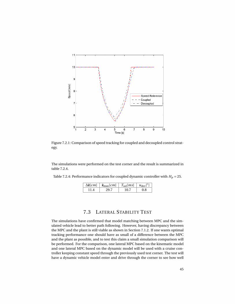
Figure 7.2.1: Comparison of speed tracking for coupled and decoupled control strat-egy.

The simulations were performed on the test corner and the result is summarized intable 7.2.4.

Table 7.2.4: Performance indicators for coupled dynamic controller with Hp = 25.

∆z[cm] zmax[cm] Tsol[ms] udev[◦]11.4 29.7 10.7 0.8

7.3 LATERAL STABILITY TEST

The simulations have confirmed that model matching between MPC and the sim-ulated vehicle lead to better path following. However, having discrepancy betweenthe MPC and the plant is still viable as shown in Section 7.1.2. If one wants optimaltracking performance one should have as small of a difference between the MPCand the plant as possible, and to test this claim a small simulation comparison willbe performed. For the comparison, one lateral MPC based on the kinematic modeland one lateral MPC based on the dynamic model will be used with a cruise con-troller keeping constant speed through the previously used test corner. The test willhave a dynamic vehicle model enter and drive through the corner to see how well

45

they complete the corner and for what speeds the path following stops performing.

The results of the simulations are shown in table 7.3.1, and an important note isthat for this test the agility of the controllers is tested and hence some comfort as-pects such as tyre slip and lateral forces/speeds will most likely be larger than theconstraints set in previous simulations. For this purpose, the controllers have beentuned individually for each speed in order to optimize the path following withoutpenalizing e.g. jerking in steering angles or tyre slip.

Table 7.3.1: Stability test during constant cornering speed

Controller v [m/s] ∆z [cm] zmax [cm] Tsol [ms] udev[◦]Kinematic 10 11.8 52.3 9.8 0.4Dynamic 10 14.3 48.9 9.9 0.4

Kinematic 11 12.6 56.3 9.9 0.6Dynamic 11 15.7 55.1 9.8 0.6

Kinematic 12 13.3 59.9 9.8 0.9Dynamic 12 17.1 61.9 9.9 0.9

Kinematic 13 16.7 63.3 9.9 2.52Dynamic 13 19.1 69.2 9.9 1.5

Kinematic 14 38.3 98.2 9.9 3.8Dynamic 14 20.8 76.8 9.8 2.1

Kinematic 15 Fails Fails Fails FailsDynamic 15 22.3 85.6 9.9 3.0

Kinematic 16 Fails Fails Fails FailsDynamic 16 Fails Fails Fails Fails

Important to not about the zmax values is that they are much larger than in the simu-lations with longitudinal controllers that can vary the speed of the vehicle. The pathwe simulate on has an optimal speed of ≈ 7 m/s which means everything above thatspeed will have trouble maintaining the perfect path throughout the corner. Whatthe stability test aims to show is how well the different controllers can recuperatefrom large path deviations due to excessive speed. The controllers that are given theflag "Fails" did not successfully re-enter the path after the corner.

7.4 SPEED PROFILE EVALUATION

In Section 5.7 a new method for creating optimal speeds for a specific path was pre-sented. The idea is to improve performance by trying to imitate the behaviour of ahuman driver when she approaches a corner. Instead of always driving at the max-imum allowed speed, the driver would instead use a piece of the straight, or nearstraight, path segment to decelerate before entering the corner. The corner wouldthen be completed using a constant speed and the acceleration out of the cornerwould be performed in a gentle way.

46

In the simulations of Chapter 7, the optimal speed has always been the maximumallowed speed for the corner. A comparison between the two different speed profilesis shown in Figure 7.4.1 and in Table 7.4.1 simulations using the best controllers ofeach strategy are summarized where the two different profiles are compared.

Figure 7.4.1: The old vmax profile compared to the new profile.

Table 7.4.1: Controller performance for two different speed profiles

Controller Profile ∆z [cm] zmax [cm] Tsol [ms] udev[◦]Kin. decoupled vmax 12.4 35.2 9.6 0.5Kin. decoupled new 10.5 33.3 8.9 0.5

Kin. coupled vmax 11.5 34.1 9.9 0.6Kin. coupled new 10.2 32.5 9.8 0.6

Dyn. decoupled vmax 9.0 25.6 9.4 0.4Dyn. decoupled new 8.4 24.5 9.6 0.6

Dyn. coupled vmax 11.4 29.7 10.7 0.8Dyn. coupled new 8.4 26.8 10.8 0.5

47

CHAPTER 8

DISCUSSION

8.1 MODEL COMPLEXITY IN MPC

A key point of the thesis is to investigate how model complexity effects the pathfollowing performance of a vehicle. It was made clear that using the same simplemodel in both the MPC and the plant would yield very accurate path following.When upping the complexity of the vehicle model both used in the MPC and theplant it showed that a more accurate MPC model will yield better path followingthan a less complex model would.

According to the simulations it was possible to use a less complex MPC model tocontrol a dynamic vehicle model in fair conditions. This was especially evident insimulations where a longitudinal controller of some sort was used and the speedinside corners was slowed down. In Section 4 it was mentioned that the kinematicvehicle and the dynamic vehicle model are in fact similar with additions of somevehicle dynamics in the bicycle model. If the dynamic terms such as vφ and vy arekept low, the bicycle model resembles the kinematic model even more. Therefore,using a longitudinal controller to keep down the velocities will open up for the useof a less complex vehicle model to control a complex vehicle. In the constant speedtest presented Table 7.3.1 it was again shown that in more extreme situations thekinematic based MPC is not good enough and the need for a more complex model isapparent. Even tough the kinematic MPC managed to complete the turn at 14 m/s,the performance indicators from both 13 and 14 m/s show that udev is considerablylarger than those of the dynamic MPC. This means that the kinematic MPC needs towork a lot harder in terms of steering angles in order to maintain the path following.

8.2 LONGITUDINAL CONTROL

To control the speed of the vehicle a longitudinal controller was added and in thedecoupled strategy this was a PI-controller while in the coupled strategy the accel-eration of the vehicle was handled by the extended MPC. In terms of speed tracking

48

and control inputs they were behaving similarly as was shown in Figure 7.2.1. Inthese specific cases the PI-controller was slower when it came to speed tracking,however this can be fixed by designing a PID-controller with optimal tuning. How-ever in this thesis the stability and path following was more important than the tra-jectory following and speed reference matching. The major advantage of having alongitudinal controller compared to travelling at constant speed is that one gets amore stable vehicle in the corners due to adapting speed.

8.3 COUPLED VS. DECOUPLED LATERAL AND

LONGITUDINAL CONTROL

Another major goal of the thesis was to design and implement a coupled lateral andlongitudinal control strategy and compare its performance against a more industrystandard decoupled approach. To perform the coupling an additional control in-put variable was added to the MPC in form of a vehicle acceleration and an onlinespeed reference calculator was added in order to feed the MPC with reference valuesfor speed and acceleration.

The first approach has an MPC based on the kinematic vehicle model and compar-ing the best performing controller in the coupled and decoupled simulation respec-tively one finds that their performance is very similar. The coupled strategy has anaverage deviation of 1 cm less than the decoupled while it also had 0.1◦ larger av-erage input deviation. This means that the lateral controller of the coupled strategyhad to work harder in order to keep the vehicle on the path. In terms of tuning andimplementation, the coupled strategy is slightly more complicated to implementthan the decoupled one.

For the coupled strategy with an MPC based on the dynamic vehicle model the im-plementation was a bit more cumbersome. Going from a lateral MPC based on thekinematic model to the dynamic model means adding three states. In the case ofcoupling one also adds a term in the equation for vx as it already exists dynamics forit in the model. If one studies Table 7.1.5 and 7.2.4 it shows that the coupled strat-egy is performing worse than the decoupled, despite having the same tuning for thelateral parts. Adding a speed tracking together with acceleration control makes theoptimization problem much more complex and one can see how the average solvertime is now almost 11 ms which is approximately 2 ms longer than the decoupledstrategy solver needs. In practice this means that the coupled control strategy vi-olates the solver constraint of 10 ms and in order to take it below 10 ms again onewould need to adjust the horizon of the MPC in order to reduce the number of itera-tion the solver runs. One can also improve the hardware by acquiring a faster PC orimprove the software and use a faster solver. The question then becomes if the cou-pled control strategy is much better than the decoupled that one can afford to lowerthe horizon without affecting its performance too much. In this case, this does notseem to be a good idea as in the simulations where we let the coupled control solver

49

run for longer, it still cannot outperform the decoupled strategy.

Much of this has to do with tuning of the longitudinal part of the MPC as it effects thelateral controller in a significant way, unlike in the coupled kinematic MPC wherethe longitudinal and lateral part were only affecting each other very slightly. Whentuning and deciding the elements of the cost matrices Q, R and P one has to thinkof how large the elements are in respect to each other. Especially important is therelation between cost elements and the state or control input they are penalizing. Ifone looks at the penalty of deviations in x position, the corresponding element ofQ has been around 100 which means a 1 cm deviation in x position will contribute100∗0.01 = 1 to the total cost function. If we look at vx it has been penalized withapproximately 1 which causes a 1 m/s deviation to contribute 1∗ 1 = 1 to the costfunction. The idea is then that deviations in x position are more important to cor-rect for the MPC rather than speed deviations. What has been complicated in thedynamic coupled strategy is the relationship between elements of Q and R where aheavy tuning on Q would lead to poor control inputs and bad path following whileheavy tuning on R would yield better control inputs but allowed for larger deviationsin states, and especially in position and orientation. The delicacy of the tuning hasproven to be tricky to handle and has lead the dynamic coupled strategy to be worseperforming than its decoupled counterpart.

8.4 USE OF A MORE CONSERVATIVE SPEED PROFILE

After running all controller simulations it became apparent how speed affects thestability of the lateral controller and general path following performance. The firstconstructed speed reference generator was based on feeding the longitudinal con-troller with the optimal speed of the current position and let it adjust the vehiclespeed accordingly. This lead to stability issues as sometimes the needed accelerationfor tracking the speed was outside the allowed bounds for the controller. In worstcase scenario when the longitudinal controller could not adapt the speed of the ve-hicle quick enough it would cause the whole vehicle to be unstable. When using thecoupled strategy one could use the fact that the horizon of the MPC could be used togive the longitudinal controller a "heads up" about upcoming speed changes. How-ever, with a horizon of 25 and a sampling time of 0.01 seconds this meant that thecontroller knew the speed approximately 2.5 meters ahead which in scenarios is notearly enough. To bypass this problem a more conservative speed profile is intro-duced and the simulations in Table 7.4.1 show how the new profile improves theoverall path following performance, and sometimes very drastically. A hidden ben-efit of the conservative speed profile is that the corners are completed with con-stant speed, which in the case of the coupled controllers meant that the MPC wasable to optimize only the steering angle in the corners and only the velocity on thestraights. By using this speed profile, one avoids the problem of constructing R andtrying to balance the relation between the two elements. In cases where the ele-ments were unbalanced, the MPC would sometimes return suboptimal values for

50

one of the control inputs. In practice, this lead to that one could have good steeringor good acceleration, but not both at the same time.

8.5 TUNING STRATEGIES

Tuning the MPC based on the kinematic model is rather straight-forward in terms ofincreasing and decreasing weights. If a reference state was not followed well enough,one could increase the weight on said state and see an immediate improvement. TheMPC based dynamic model was slightly more complicated as it had more dynamicsand increasing one weight in the cost matrices could affect another state referenceas well. For the dynamic MPC, the relation between the weights was equally im-portant as the size of individual weights. An interesting finding was that the pathfollowing would perform worse when the elements of Q and P were too large . Inone simulation on a dynamic lateral MPC, two new tunings were tested: controller2 and controller 3. The controllers had the same R matrices, but the elements of Pand Q in controller 2 was three times larger than those of controller 3. In Figure 8.5.1the path taken and the steering angle inputs from controller 2 and 3 is shown. Fromthe data one can see how the controller 2 deviates much from reference steering an-gle and swivels along the path. Compared to controller 3 where the elements of Pand Q is smaller, the steering angle deviations and the path deviations are reducedas shown in figure 8.5.1a and the steering angle follows the reference input closer asseen in Figure 8.5.1b. The results show that simply increasing the weights will notnecessarily improve performance.

50 52 54 56 58 60

5

6

7

8

9

10

11

12

13

x−position

y−po

sitio

n

Controller 3Controller 2Path boundries

(a) Comparison of path taken.

1 2 3 4 5 6 7 8 9 10−5

0

5

10

15

20

25

30

35

Time [s]

Ste

erin

g A

ngle

[deg

]

Controller 3 InputController 2 InputInput Reference

(b) Difference in control input.

Figure 8.5.1: Comparison between controller 2 and controller 3

8.6 COMMENTS ON THE COMPLETE SYSTEM

For this autonomous vehicle system we introduced four different control strategies:coupled and decoupled control based on kinematic and dynamic vehicle models.

51

The decoupled strategies with PI-controller for longitudinal control were the easi-est to implement where the MPC problem only focused on lateral dynamics. Thekinematic MPC was able to control a dynamic vehicle model but the dynamic MPCperformed better than the kinematic. The coupled control strategy performed verywell, especially with the more conservative speed profile. However, tuning and set-ting up the coupled control is significantly more cumbersome compared to the de-coupled strategy. In Figure 8.6.1 the four control strategies have been evaluated in a"triangle-form". The black dot represents how the control strategies is relative to thethree corners of the triangle. The corners are: easy setup, which means how easy it isto tune and use the strategy, Time, which describes how fast the control strategy canbe solved by an MPC solver, and performance, which accounts for path and controldeviations. Note that all four control strategies did perform good path following, andthe performance indicator for one strategy is relative to the others. The kinematicstrategies are closer to time and easy setup while the dynamic strategies are closerto performance but farther away from easy setup. The coupled control strategies areas well more difficult to tune and implement than their decoupled counterpart.

Figure 8.6.1: Evaluation of the four control strategies for an autonomous vehicle.

52

CHAPTER 9

CONCLUSION

This work has demonstrated the effectiveness of an MPC based path and trajectoryfollowing control for autonomous vehicles. Stable and well performing MPC lateralcontrollers have been developed and tested and served as the base for developingthe whole autonomous system. The lateral MPC controllers have performed well inthe tasks of path and trajectory following and due to the great customization abil-ity of the controller. The used tuning strategies have given stable controllers whichalso have proven to be robust enough to allow for model discrepancies. This workhas seen that MPC controllers based on simplified models can still work on morecomplex vehicle models which has allowed for fast solver times as well as easy im-plementation. Using more advanced vehicle models as base for the MPC does yieldbetter performance in terms of stability and tracking, but in many circumstancesthe basic MPC is performing well enough that the extra solver time and added com-plexity of more advanced MPC might in some cases not be needed.

The developed coupled control strategy for lateral and longitudinal control has per-formed slightly better than the decoupled strategy. The advantage of having onecoupled control system with one complex MPC is the small performance improve-ment as well as overall system simplicity in only having one controller for the vehi-cle. The set-up and tuning of the coupled strategy is however more complex thanthe decoupled strategy and the risk of suboptimal control inputs due to incorrecttuning has proven to be a drawback.

In terms of creating a complete system for autonomous vehicles there has been is-sues of performance. The functions for finding reference inputs in both speed, ac-celeration and steering angle are all basic and static functions. The performance ofthe complete vehicle control system is held back by its weakest link. If the speedreference function for instance fails and outputs poor reference values, there is noguarantee that any of the control strategies would keep the vehicle on the road. Thefocus of this paper has been on developing and tuning the lateral and longitudinalcontrollers, but experience from the implementation and simulations have shownthat equal amount of attention should be given to the actual path and the informa-

53

tion the vehicle can extract from it. The improved speed profile is a result of thisinsight and the increased complexity of the new speed profiler showed great resultsin terms of performance and vehicle stability.

The most complex, non-control related task is the waypointing and path finding. Inthis thesis there was only one available path but the vehicle had to work out whichwaypoints to follow. The solution for this was to work with a discretization of thepath and then run an algorithm to solve for the appropriate waypoints. The majordrawback of this approach was the size of the discretized path. The path in which thesimulations were made consisted of thousands of available waypoints and runningthe algorithm in its current state was slower than the MPC solver. In the simulationsthe waypointing was excluded from all time measurements with the reasoning thata well-written and optimized waypoint finding algorithm would not be as resourceheavy as the current version. The topics of path finding and waypointing were toogreat to be researched properly in this thesis and focus was hence laid on lateral andlongitudinal control.

54

CHAPTER 10

FUTURE WORK

IMPLEMENTATION

The next step for testing the work of this thesis is to implement the controllers on ei-ther downscaled model vehicles or a full size one. This will include optimizing otherparts of the control such as reference generating, path finding and waypointing tomake it work in real time.

TUNING

The main tuning strategy for all controllers have been trial-and-error which was verytime consuming for the more complex MPC controllers. Finding a method for tun-ing and optimizing the MPC is also a field one can investigate further.

WAYPOINTING AND PATH FINDING

Finally, a large topic which was not covered in depth was path finding and way-pointing. Developing smart and efficient algorithms that work well with the fullautonomous system would be interesting as some results have pointed to that thequality of the information fed to the controllers have a drastic effect on performance.Creating a path finder that can replan a route online and perhaps avoid obstacleswould improve the overall performance of the suggested control strategies.

55

BIBLIOGRAPHY

[1] Ralph R Teetor. Vehicle speed maintaining and maximum speed controllingdevice, December 8 1959. US Patent 2,916,100.

[2] J. Markoff. Google Cars Drive Themselves, in Traffic. Retrived 2015-05-11.http://www.nytimes.com/2010/10/10/science/10google.html, 2010.

[3] J. Ramey. Watch an Autonomous Audi RS7 Fly Around the HockenheimCircuit. Retrived 2015-05-18. http://autoweek.com/article/car-news/

watch-audis-autonomous-rs-7-fly-around-hockenheim-circuit,2014.

[4] J. Ziegler Et. al. Making Bertha drive - an autonomous journey on a historicroute. IEEE Intelligent Transportation Systems Maganize, 2014.

[5] F. Kühne, W.F. Lages, and JM GOMES da SILVA. Mobile robot trajectory trackingusing model predictive control. In II IEEE latin-american robotics symposium,2005.

[6] T. Keviczky, P. Falcone, F. Borrelli, J. Asgari, and D. Hrovat. Predictive controlapproach to autonomous vehicle steering. In American Control Conference,2006, pages 6 pp.–, June 2006.

[7] P. Falcone, F. Borrelli, H.E. Tsengz, J. Asgari, and D. Hrovat. A hierarchical modelpredictive control framework for autonomous ground vehicles. In AmericanControl Conference, 2008, pages 3719–3724, June 2008.

[8] P. Falcone, F. Borrelli, J. Asgari, H.E. Tseng, and D. Hrovat. A real-time modelpredictive control approach for autonomous active steering. Nonlinear ModelPredictive Control for Fast Systems, Grenoble, France, 2006.

[9] V. Turri, A. Carvalho, H. Tseng, K.H. Johansson, and F. Borrelli. Linear modelpredictive control for lane keeping and obstacle avoidance on low curvatureroads. In 2013 16th International IEEE Conference on Intelligent Transporta-tion Systems: Intelligent Transportation Systems for All Modes, ITSC 2013; TheHague; Netherlands; 6 October 2013 through 9 October 2013, pages 378–383.IEEE, 2013.

56

[10] P. Falcone, F. Borrelli, J. Asgari, H.E. Tseng, and D. Hrovat. Predictive activesteering control for autonomous vehicle systems. Control Systems Technology,IEEE Transactions on, 15(3):566–580, May 2007.

[11] E. Bakker, L. Nyborg, and H.B. Pacejka. Tyre modelling for use in vehicle dy-namics studies. Technical report, SAE Technical Paper, 1987.

[12] R. Attia, R. Orjuela, and M. Basset. Combined longitudinal and lateral controlfor automated vehicle guidance. Vehicle System Dynamics, 52(2):261–279, 2014.

[13] R. Attia, Rodolfo O., and M. Basset. Coupled longitudinal and lateral controlstrategy improving lateral stability for autonomous vehicle. In American Con-trol Conference (ACC), 2012, pages 6509–6514. IEEE, 2012.

[14] P. Lima, M. Trincavelli, and J. Martensson. Clothoid-based model predictivecontrol for autonomous driving. 2015.

[15] S. Nordmark E. Wennerström and B. Thorvald. Vehicle dynamics course com-pendium, 2011. KTH Vehicle Dynamics, Aeronautical and Vehicle Engineering.

[16] F. Holzmann, B. Chrétien, H. Zeng, T. Gallner, and G. Spiegelberg. Integratedlongitudinal and lateral controls on drive-by-wire platform to improve the roadsafety. In SAE Technical Paper. SAE International, 04 2008.

[17] T. Glad and L. Ljung. Reglerteknik: Grundläggande teori. Studentlitteratur AB,2006.

[18] T. Glad and L. Ljung. Reglerteknik: Flervariabla och olinjära metoder. Stu-dentlitteratur AB, 2003.

[19] C. Jones. An introduction to model predictive control. University Lecture atÉcole Polytechnique Fédérale de Lausanne, 2014.

[20] C. Jones. Practical MPC. University Lecture at École Polytechnique Fédérale deLausanne, 2014.

[21] A. Howard and C. Rorres. Elementary Linear Algebra with Applications, 8th Ed.2009.

[22] C. Jones. Introduction to convex optimization. University Lecture at École Poly-technique Fédérale de Lausanne, 2014.

[23] J. McCrae and K. Singh. Sketching piecewise clothoid curves. Computers &Graphics, 33(4):452–461, 2009.

[24] J. Mattingley and S. Boyd. Cvxgen: a code generator for embedded convex op-timization. Optimization and Engineering, 13(1):1–27, 2012.

[25] J. Mattingley, Y. Wang, and S. Boyd. Receding horizon control. Control Systems,IEEE, 31(3):52–65, 2011.

57

TRITA XR-EE-RT 2015:013

ISSN 1653-5146

www.kth.se